Relaxation Subgradient Algorithms with Machine Learning Procedures ^†

Abstract

In the modern digital economy, optimal decision support systems, as well as machine learning systems, are becoming an integral part of production processes. Artificial neural network training as well as other engineering problems generate such problems of high dimension that are difficult to solve with traditional gradient or conjugate gradient methods. Relaxation subgradient minimization methods (RSMMs) construct a descent direction that forms an obtuse angle with all subgradients of the current minimum neighborhood, which reduces to the problem of solving systems of inequalities. Having formalized the model and taking into account the specific features of subgradient sets, we reduced the problem of solving a system of inequalities to an approximation problem and obtained an efficient rapidly converging iterative learning algorithm for finding the direction of descent, conceptually similar to the iterative least squares method. The new algorithm is theoretically substantiated, and an estimate of its convergence rate is obtained depending on the parameters of the subgradient set. On this basis, we have developed and substantiated a new RSMM, which has the properties of the conjugate gradient method on quadratic functions. We have developed a practically realizable version of the minimization algorithm that uses a rough one-dimensional search. A computational experiment on complex functions in a space of high dimension confirms the effectiveness of the proposed algorithm. In the problems of training neural network models, where it is required to remove insignificant variables or neurons using methods such as the Tibshirani LASSO, our new algorithm outperforms known methods.

1. Introduction

In this study, which is an extension of previous work [1], a problem of minimizing a convex, not necessarily differentiable function $f\left(x\right),x\in {\mathbb{R}}^n$ (where ${\mathbb{R}}^n$ is a finite-dimensional Euclidean space) is discovered. Such a problem is quite common in the field of machine learning (ML), where optimization methods, in particular, gradient descent, are widely used to minimize the loss function during training stage. In the era of the digital economy, such functions arise in many engineering applications. First of all, training and regularizing the artificial neural networks of a simple structure (e.g., radial or sigmoidal) may lead to the application of a loss function in a high-dimensional space, which are often non-smooth. When working with more complex networks, such functions can be non-convex.

While a number of efficient machine learning tools exist to learn smooth functions with high accuracy from a finite data sample, the accuracy of these approaches becomes less satisfactory for nonsmooth objective functions [2]. In a machine learning context, it is quite common to have an objective function with a penalty term that is non-smooth such as the Lasso [3] or Elastic Net [4] linear regression models. Common loss functions, such as the hinge loss [5] for binary classification, or more advanced loss functions, such as the one arising in classification with a reject option, are also nonsmooth [6], as well as some widely used activation functions (ReLU) [7] in the field of deep learning. Modern convolutional networks, incorporating rectifiers and max-pooling, are neither smooth nor convex. However, the absence of differentiability creates serious theoretical difficulties on different levels (optimality conditions, definition and computation of search directions, etc.) [8].

Modern literature offers two main approaches to building nonsmooth optimization methods. The first is based on creating smooth approximations for nonsmooth functions [9,10,11,12,13]. On this basis, various methods intended for solving convex optimization problems, problems of composite and stochastic composite optimization [9,10,11,14] were theoretically substantiated.

The second approach is based on subgradient methods that have their origins in the works of N. Z. Shor [15] and B.T. Polyak [16], the results of which can be found in [17]. Initially, relaxation subgradient minimization methods (RSMMs) were considered in [18,19,20]. They were later developed into a number of effective approaches such as the subgradient method with space dilation in the subgradient direction [21,22] that involve relaxation by distance to the extremum [17,23,24]. The idea of space dilation is to change the metric of the space at each iteration with a linear transformation and to use the direction opposite to that of the subgradient in the space with the transformed metric.

Embedding the ideas of machine learning theory [25] into such optimization methods made it possible to identify the principles of organizing RSMM with space dilation [26,27,28,29]. The problem of finding the descent direction in the RSMM can be reduced to the problem of solving a system of inequalities on subgradient sets, mathematically formulated as a problem of minimizing a quality functional. This means that a new learning algorithm is embedded into the basis of some new RSMM algorithm. Thus, the convergence rate of the minimization method is determined by the properties of the learning algorithm.

Rigorous investigation of the approximation capabilities of various neural networks has received much research interest [30,31,32,33,34,35,36] and is widely applied to problems of system identification, signal processing, control, pattern recognition and many others [37]. Due to universal approximation theorem [30], a feedforward network with a single hidden layer and a sigmoidal activation function can arbitrarily well approximate any continuous function on a compact set [38]. The studies of learning theory on unbounded sets can be found in [39,40,41].

The stability of the neural network solutions can be improved by introducing a regularizing term in the minimized functional [42], which stabilizes the solution using some auxiliary non-negative function carrying information on the solution obtained earlier (a priori information). The most common form of a priori information is the assumption of the function smoothness in the sense that the same input signal corresponds to the same output. Commonly used regularization types include:

1. Quadratic Tikhonov regularization (or ridge regression, $R_2$). In the case of approximation by a linear model, the Tikhonov regularizer [42] is used:

$$R_2\left(U\right)=\sum _{i=1}^k{u}_i^2,$$

(1)

where parameters of the linear part of the model are included, and k is the number of vector U components. The regularizer $R_2$ is mainly used to suppress large components of the vector U to prevent overfitting the model.

2. Modular linear regularization (Tibshirani Lasso, $R_1$). The regularizer proposed in [3] is mainly used to suppress large and small components of the vector U:

$$R_1\left(U\right)=\sum _{i=1}^k\left|u_i\right|.$$

(2)

3. Non-smooth regularization ($R_{\gamma }$) [3,43]:

$$R_{\gamma }\left(U\right)=\sum _{i=1}^k\left(\right|u_i{|+\epsilon )}^{\gamma },\epsilon ={10}^{-6},\gamma =0.7.$$

(3)

The use of $R_{\gamma }$ led to the suppression of small (“weak”) components of the vector U. This property of $R_{\gamma }$ enables us to reduce to zero weak components that are not essential for the description of data.

The aim of our work is to outline an approach to accelerating the convergence of learning algorithms in RSMM with space dilation and to give an example of the implementation of such an algorithm, confirming the effectiveness of theoretical constructions.

In the RSMM, successive approximations [18,19,20,26,28,44] are:

$$x_{k+1}=x_k-{\gamma }_k{s}_{k+1},{\gamma }_k=arg\underset{\gamma }{min}f(x_k-\gamma s_{k+1}),$$

(4)

where k is the iteration number, ${\gamma }_k$ is the stepsize, $x_0$ is a given starting point, and the descent direction $s_{k+1}$ is a solution of a system of inequalities on $s\in {\mathbb{R}}^n$ [20]:

$$(s,g)>0,\forall g\in G.$$

(5)

Hereinafter, $(s,g)$ is a dot product of vectors, and G is a set of subgradients calculated on the descent trajectory of the algorithm at a point $x_k$.

Denote as $(s,g)$ a set of solutions to inequality (5), as $\partial f\left(x\right)$ is a subgradient set at point x. If the function is convex and $G={\partial }_{\epsilon }f\left(x_k\right)$ is an $\epsilon$-subgradient set at point $x_k$, and $s_{k+1}$ is an arbitrary solution of system (5), then the function will be reduced by at least $\epsilon$ after iteration (4) [20].

Since there is no explicit specification of $\epsilon$-subgradient sets, the subgradients $g_k\in \partial f\left(x_k\right)$ are used as elements of the set G, calculated on the descent trajectory of the minimization algorithm. These vectors must satisfy the condition:

$$(s_k,g_k)\le 0.$$

(6)

Inequality (6) means that for the vectors used, condition (5) is not satisfied. The choice of learning vectors is made according to this principle in the perceptron method [25,45], for instance.

A sequence of vectors $g_k\in \partial f\left(x_k\right),k=0,1,\dots$ is not predetermined, but determined during minimization (4) with a built-in method for finding the vector $s_{k+1}$ at each iteration of minimization by a ML algorithm.

Let vector $s_{k+1}$ be a solution of the system of inequalities (5) for the subgradient set of some neighborhood of the current minimum $x_k$. Then, as a result of iteration (4), we go beyond this neighborhood with a simultaneous function decrease, since vector $s_{k+1}$ forms an acute angle with each of the subgradients of the set.

In this work, we present a formalized model of subgradient sets, which enables us, taking into account their specificity, to formulate stronger learning relations and quality functionals, which leads to acceleration in the convergence rate of learning algorithms designed to form the direction of descent in the RSMM.

As a result of theoretical analysis, an effective learning algorithm has been developed. For the proposed ML algorithm, the convergence in a finite number of iterations is proved when solving problem (5) on separable sets. Based on the learning algorithm, we proposed a method for minimizing nonsmooth functions. Its convergence on convex functions was substantiated. It is shown that on quadratic functions, the minimization method generates a sequence of minimum approximations identical to the sequence of the conjugate gradient method. We also proposed a minimization algorithm with a specific one-dimensional search method. A computational experiment confirmed its effectiveness for problems of neural network approximations, where the technology of uninformative model component suppression with regularizers similar to the Tibshirani LASSO was used [46]. The result of our work is an optimization algorithm applicable for solving neuron network regularization and other machine learning problems which, in turn, contains an embedded machine learning algorithm for finding the most promising descent direction. In the problems used for comparison, the objective function forms an elongated multidimensional ravine. As with other subgradient algorithms, our new algorithm proved to be efficient for such problems. Moreover, the new algorithm outperforms known relaxation subgradient and quasi-Newtonian algorithms.

The rest of this article is organized as follows. In Section 2, we consider a problem of acceleration of the learning algorithms convergence using relaxation subgradient methods. In Section 3, we make assumptions regarding the parameters of subgradient sets that affect the convergence rate of the proposed learning algorithm. In Section 4, we formulate and justify a machine learning algorithm for finding the descent direction in the subgadient method. In Section 5, we give a description of the minimization method. In Section 6, we establish the identity of the sequences generated by the conjugate gradient method and the relaxation subgradient method with space dilation on the minimization of quadratic functions. In Section 7 and Section 8, we consider a one-dimensional minimization algorithm and its implementation, respectively. In Section 9 and Section 10, we present experimental results for the considered algorithms. In Section 9, we show a computational experiment on complex large-sized function minimization. In Section 10, we consider experiments with training neural network models, where it is required to remove insignificant neurons. Section 11 contains a summary of the work.

2. Acceleration of the Learning Algorithm’s Convergence in Relaxation Subgradient Methods

To use more efficient learning algorithms, a relation stronger than (5) can be written for the descent direction. We make an additional assumption about the properties of the set G.

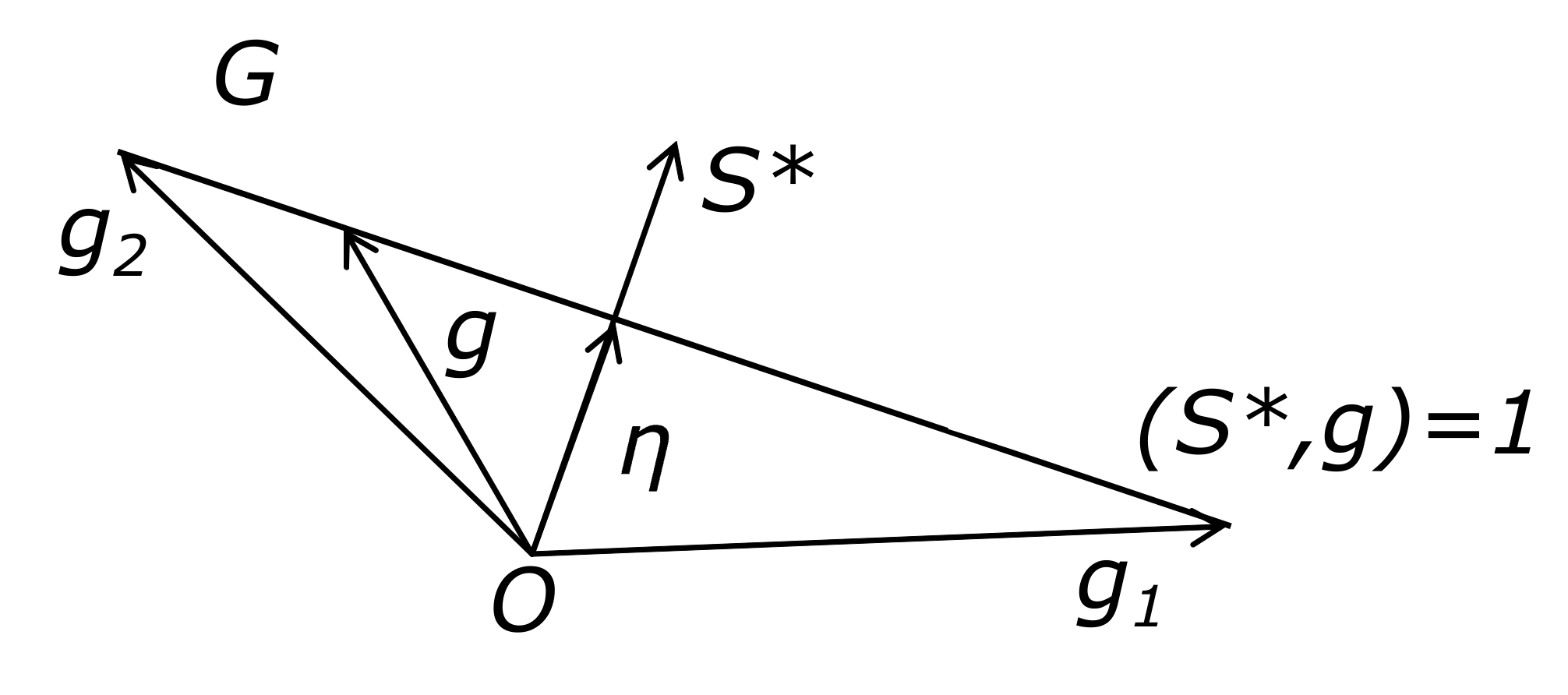
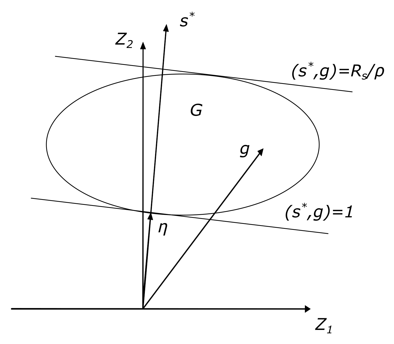
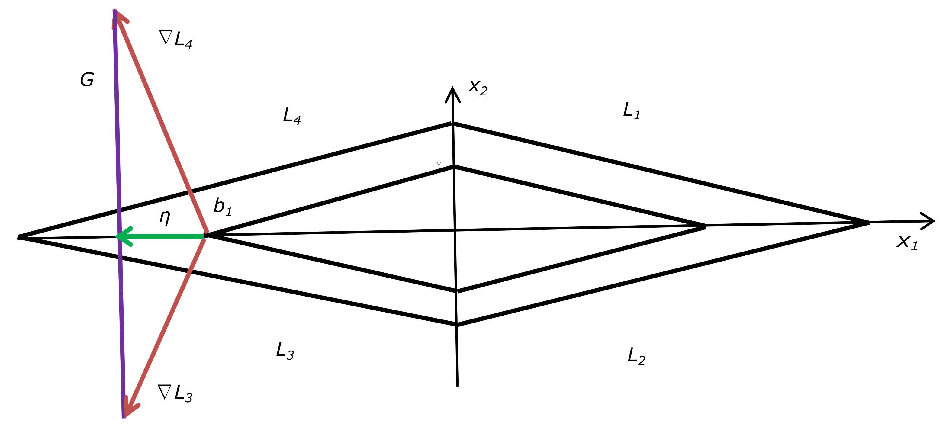
Assumption 1. 

Let a convex set $G\subset {\mathbb{R}}^n$ belong to a hyperplane; its minimal length vector η is also the minimal length vector of this hyperplane. Then, a solution of the system $(s,g)=1\forall g\in G$ is also a solution of (5) [26]. It can be found as a solution to a system of equations using a sequence of vectors from G [26]:

$$(s,g_i)=q_i=1,g_i\in G,i=0,1,\dots k.$$

(7)

It is easy to see that the solution to system (7) in s is the vector $s^{\ast }=\eta /{\left|\right|\eta \left|\right|}^2$. Figure 1 shows the subgradient set in the form of a segment lying on a straight line. Equalities (7) can be solved by a least squares method. For example, using the quadratic quality functional

$$Q_k\left(s\right)=\frac{1}{2}{(1-(s,g_k))}^2,$$

it is possible to implement a gradient machine learning algorithm,

$$s_{k+1}=s_k-{\beta }_k\nabla Q_k\left(s_k\right),$$

where ${\beta }_k$ is a gradient method step. Hence, when choosing ${\beta }_k=1/(g_k,g_k)$, we obtain the well-known Kaczmarz algorithm [47],

$$s_{k+1}=s_k+\frac{1-(s_k,g_k)}{(g_k,g_k)}{g}_k.$$

(8)

The found direction $s_k$ satisfies the learning equality $(s_{k+1},g_k)=1$. To ensure the possibility of decreasing the function as a result of iteration (4), the new descent direction in the minimization method must be consistent with the current subgradient, i.e., satisfy inequality $(s_{k+1},g_k)>0$. Process (8) corresponds to this condition.

To propose a faster algorithm, consider the interpretation of process (8). Let Assumption 1 be fulfilled. The step of process (8) is equivalent to the step of one-dimensional minimization of the function

$$E\left(s\right)=\frac{(s-s^{\ast },s-s^{\ast })}{2}$$

from point $s_k$ in the direction $g_k$. Let the current approximation $s_k$ be obtained using a vector $g_{k-1}$ and satisfy the condition $(s_k,g_{k-1})=1$. Figure 2 shows the projections of the current approximation $s_k$ and the required vector $s^{\ast }$ on the plane of vectors $g_{k-1},g_k$. Straight lines $W_1$ and $Z_1$ are hyperplane projections for vectors s, given by the equalities $(s,g_{k-1})=1$ and $(s,g_k)=1$. Vector $s_{k+1}^1$ is a projection of the approximation obtained from the iteration (8).

If $(g_k,g_{k-1})\le 0$, then the angle between subgradients is obtuse, and the angle $\phi$ is acute (Figure 2). In this case, it is possible to completely extinguish the projection of the residual between $s_k$ and $s^{\ast }$ in the plane of vectors $g_{k-1},g_k$, passing from point A to point C along vector $AC$, perpendicular to the vector $g_{k-1}$, i.e., along vector $p_k$:

$$p_k=g_k-g_{k-1}\frac{(g_k,g_{k-1})}{(g_{k-1},g_{k-1})}.$$

(9)

In this case, the iteration has the form

$$s_{k+1}=s_k+p_k\frac{1-(s_k,g_k)}{(g_k,p_k)}.$$

(10)

In Figure 2, this vector is denoted as $s_{k+1}^2$. The vector $s_{k+1}$, obtained by formula (10), satisfies the equalities $(s_{k+1},g_{k-1})=1$, $(s_{k+1},g_k)=1$ and coincides with the projection $s^{\ast }$ of the optimum of the function $E\left(s\right)$. At small angles $\varphi$ between the straight lines $W_1$ and $Z_1$, the acceleration of convergence for process (10) becomes essential. In this work, process (10) will be used to accelerate the convergence in the metric of the iterative least squares method.

Using learning information (7), one of the possible solutions to the system of inequalities (5) can be found in the form $s_{k+1}=arg{min}_s{F}_k\left(s\right)$, where

$$F_k\left(s\right)=\sum _{i=0}^k{w}_i{Q}_i\left(s\right)+\frac{1}{2}\sum _{i=1}^n{s}_i^2,Q_i\left(s\right)=\frac{1}{2}{(q_i-(s,g_i))}^2.$$

Such a solution can be obtained by the iterative least squares method (ILS). With weight factors $w_i=1$, after the arrival of new data $q_k,g_k$, the transition from the previously found solution $s_k$ to a new solution $s_{k+1}$ in ILS is made as follows:

$$s_{k+1}=s_k+\frac{H_k{g}_k(q_k-(s_k,g_k))}{1+(H_k{g}_k,g_k)},s_0=0,$$

(11)

$$H_{k+1}=H_k-\frac{H_k{g}_k{g}_k^T{H}_k^T}{1+(g_k,H_k{g}_k)},H_0=I.$$

(12)

Note that, in contrast to the usual ILS, there is a regularizing component ${\sum }_{i=1}^n{s}_i^2/2$ in $F_k\left(s\right)$, which allows us to use transformations (11) and (12) from the initial iteration, setting $s_0=0$ and $H_0=I$.

In [26], based on ILS (11) and (12), an iterative process is proposed for solving the system of inequalities (5) using learning information (7):

$$s_{k+1}=s_k+\frac{H_k{g}_k[1-(s_k,g_k)]}{(g_k,H_k{g}_k)},s_0=0,$$

(13)

$$H_{k+1}=H_k-(1-\frac{1}{{\alpha }_k^2})\frac{H_k{g}_k{g}_k^T{H}_k^T}{(g_k,H_k{g}_k)},H_0=I.$$

(14)

Here, ${\alpha }_k>1$ is a space dilation parameter.

Consider the rationale for the method of obtaining formulas (13) and (14). Using processes (11) and (12) for scaled data, we obtain

$$\widehat{g_k}=g_k{\left[q(g_k,H_k{g}_k)\right]}^{-0.5},\widehat{q_k}=q_k{\left[q(g_k,H_k{g}_k)\right]}^{-0.5},$$

where scaling factor $q>0$. The latter is equivalent to introducing the weight factors $w_k=1/\left[q(g_k,H_k{g}_k)\right]$ in $F\left(s\right)$. Then, after returning to the original data $g_k,y_k$, we obtain the expressions:

$$s_{k+1}=s_k+\frac{H_k{g}_k[q_k-(s_k,g_k)]}{(1+q)(g_k,H_k{g}_k)},s_0=0,$$

(15)

$$H_{k+1}=H_k-\frac{H_k{g}_k{g}_k^T{H}_k^T}{(1+q)(g_k,H_k{g}_k)},H_0=I.$$

(16)

The transformation of matrices (16) is practically equivalent to (14) after the appropriate choice of the parameter q. For transformation (15), the condition $(s_{k+1},g_k)>0$ providing the condition for the possibility of decreasing the function in the course of iteration (4) along the direction $s_{k+1}$ may not be satisfied. Therefore, the transformation (13) is used with $q_k=1$, which ensures equality $(s_{k+1},g_k)=1>0$. Transformation (13) can be interpreted as the Kaczmarz algorithm in the corresponding metric. As a result, we obtain processes (13) and (14). Methods [18,19,20] of the class under consideration possess the properties of the conjugate gradient method. The noted properties expand the area of effective application of such methods.

The higher the convergence rate of processes (13) and (14), the greater the value of the permissible value ${\alpha }_k$ in (14) [26], which depends on the set G’s characteristics. In algorithms (13) and (14), we distinguish 2 stages: the correction stage (13). reducing the residual between the optimal solution $s^{\ast }$ and the current approximation $s_k$, and the space dilation stage (14), resulting in the increase in the residual in the transformed space without exceeding its initial value, which limits the magnitude of the space dilation parameter. To create more efficient algorithms for solving systems of inequalities, we have to choose the direction of correction in such a way that the reduction of the residual is higher than that of process (13). The direction of space dilation should be chosen so that it becomes possible to increase the space dilation parameter value due to this choice.

This paper presents one of the special cases of the implementation of the correction stage and space dilation stage. It was proposed to use linear combinations of vectors $g_{k-1},g_k$ in transformation (13) instead of a vector $g_k$ when it is appropriate:

$$p_k=g_k-g_{k-1}\frac{(g_k,H_k{g}_{k-1})}{(g_{k-1},H_k{g}_{k-1})},$$

(17)

$$s_{k+1}=s_k+H_k{p}_k\frac{1-(s_k,g_k)}{(g_k,H_k{p}_k)}.$$

(18)

Transformations (17) and (18) are similar to the previously discussed transformations (9) and (10) carried out in the transformed space.

In the matrix transformation, we use equation (14) instead of vector $g_k$. We also use vector $y_k=g_k-g_{k-1}$ such that

$$H_{k+1}=H_k-(1-\frac{1}{{\alpha }_k^2})\frac{H_k{y}_k{y}_k^T{H}_k^T}{(y_k,H_k{y}_k)}.$$

(19)

As shown below, the discrepancy between the optimal solution $s^{\ast }$ and the current approximation $s_{k+1}$ along the vector $y_k$ is small, which makes it possible to use large parameters of space dilation ${\alpha }_k$ in (19). Iterations (18) and (19) are conducted under the condition:

$$(g_k,H_k{g}_{k-1})\le 0.$$

(20)

In the next section, assumptions will be made regarding the parameters of subgradient sets that affect the convergence rate of the proposed learning algorithm and determine the permissible parameters of space dilation. This allows us to formulate and justify a machine learning algorithm for finding the descent direction in the subgradient method. Note that the described parameterization of the sets does not impose any restrictions on the subgradient sets but is used only for the purpose of developing constraints on the learning algorithm parameters.

3. Formalization of the Separable Sets Model

In this section, we will use the following notation (as earlier, vector $\eta$ is the shortest vector from G):

(1)

$\rho =\left|\right|\eta \left|\right|$ is the length of the minimal vector of the set;

(2)

$R={max}_{g\in G}\left|\right|g\left|\right|$ is the length of the maximal vector of the set;

(3)

$\mu =\eta /\rho$ is the normalized vector $\eta$;

(4)

$s^{\ast }=\mu /\rho$ is a vector associated with the sought solution of systems (5) and (7) when analyzing the ML algorithm;

(5)

$R_s={max}_{g\in G}(\mu ,g)$ is an upper-bound value of the set G in the direction $\mu$;

(6)

$M=R_s/\rho$ is the ratio of the upper and lower bounds of the set along $\mu$, $r=\rho /R_s=M^{-1}$;

(7)

$V=\rho /R$ is the ratio of the minimal and maximal vectors of the set.

For some set Q, we will use the noted characteristics indicating the set as an argument; for example, $\eta \left(Q\right),r\left(Q\right)$.

We assume that set G satisfies the assumption:

Assumption 2 

([1]). Set G is convex, closed, limited $(R<\infty )$ and satisfies the separability condition, i.e., $\rho >0$.

Vector $s^{\ast }$ is a solution to the system of inequalities (5), and ρ and $R_s$ describe the thickness of the set G in the direction μ:

$$\rho \le (\mu ,g)\le R_s,\forall g\in G.$$

(21)

Due to (21) and the form of $s^{\ast }$:

$$1\le (s^{\ast },g)\le R_s/\rho =M,\forall g\in G.$$

(22)

$R_s$, according to its definition, satisfies the constraints:

$$\rho \le R_s\le \left|\right|\mu \left|\right|\underset{g\in G}{max}\left|\right|g\left|\right|\le R.$$

Figure 3 shows a separable set and its characteristics. The $R_s$ characteristic determines the thickness of the set G and significantly affects the convergence rate of learning algorithms with space dilation. When the thickness of the set is equal to zero, $R_s=\rho$ and a flat set takes place (Figure 1). Set G and its characteristics with boundaries (22) are shown in Figure 3.

For example, consider the function

$$f\left(x\right)=\sum _{i=1}^n\left|x_i\right|a_i,a_i\ge 0,i=1,\dots ,n,x^0=(b_1,\dots ,b_m,0,\dots ,0).$$

(23)

The point $x^0$ is located at the bottom of a multidimensional ravine. Let us study its subgradient set at point $x^0$. As earlier, $g\left(x^0\right)$ is subgradient of a function. Components of subgradient vectors at non-zero values $x_i$ are as follows: $g_i\left(x\right)=sign\left(x_i\right)a_i$. For zero $x_i$, the components of the subgradient vectors belong to the set $g_i\left(x\right)\in [-a_i,a_i]$, where the zero component $g_i\left(x\right)=0$ exists. Hence, it follows that the subgradient of the minimum length of function (23) at point $x^0$ has the form

$$\eta =g_{min}^0=(sign\left(b_1\right)a_1,\dots ,sign\left(b_m\right)a_m,0,\dots ,0).$$

Maximum length subgradients are specified by a set of subgradients

$$g_{max}^0\in G=\left\{(sign\left(b_1\right)a_1,\dots ,sign\left(b_m\right)a_m,\pm a_{m+1},\dots ,\pm a_n)\right\}.$$

It is easy to verify that the projections of arbitrary subgradients at the point $x_0$ onto vector $g_{min}^0$ are the same. Therefore, the thickness of the subgradient set is zero. In a sufficiently small neighborhood of the point $x^0$, the union of the subgradient sets of function (23) coincides with the subgradient set at the point $x^0$. Consequently, the descent direction in the form of a solution to the system of inequalities (7) enables us to go beyond this neighborhood.

Figure 4 shows a representation of the subgradient set of a two-dimensional piecewise linear function

$$f\left(x\right)=|x_1|+|x_2|a,a>1,x^0=(b_1,0).$$

(24)

In quadrants, the function has the form

$$L_1\left(x\right)=x_1+x_{2}a,L_2\left(x\right)=x_1-x_{2}a,L_3\left(x\right)=-x_1-x_{2}a,L_4\left(x\right)=-x_1+x_{2}a.$$

Its subgradients at point $x^0$ are given as follows:

$$g_1\left(x^0\right)=\nabla L_3\left(x^0\right)={(-1,-a)}^T,g_2\left(x^0\right)=\nabla L_4\left(x^0\right)={(-1,a)}^T.$$

Minimum length vector $\eta ={(-1,0)}^T$.

For large values of the parameter a in (24), the complexity of solving the minimization problem increases significantly.

4. Machine Learning Algorithm with Space Dilation for Solving Systems of Inequalities on Separable Sets

In this section, we briefly introduce an algorithm for solving systems of inequalities from [1] and theoretically justify iterations (18) and (19). Specific operators will be used for transformations (13), (14) and (17)–(19). Denote by $S(s,g,p,H)$ transformation (18)’s operator, where the correspondence is used for the eponymous components. Then, for example, Formula (13) can be represented as $s_{k+1}=S(s_k,g_k,g_k,H_k)$. Similarly, for (14) and (19), we introduce the operator $H(H,\alpha ,g)$. Formula (19) can be represented as $H_{k+1}=H(H_k,{\alpha }_k,y_k)$.

For a chain of approximations $s_k$, we form the residual vector ${\Delta }_k=s^{\ast }-s_k$. Until vector $s_k$ is not a solution to (5), for vectors $g_k$ selected at step 2 of Algorithm 1, from (6) and (22), the following inequality holds:

$$({\Delta }_k,g_k)=(s^{\ast }-s_k,g_k)=(s^{\ast },g_k)-(s_k,g_k)\ge 1-(s_k,g_k)\ge 1.$$

(25)

The transformation equation for matrix $A_k$ is as follows [1]:

$$A_{k+1}=A_k+({\alpha }^2-1)\frac{g_k{g}_k^T}{(g_k,H_k{g}_k)},$$

(26)

$$A_{k+1}=A_k+({\alpha }_k^2-1)\frac{y_k{y}_k^T}{(y_k,H_k{y}_k)},$$

(27)

where $A_k=H_k^{-1}$. For vectors $s_k$ and $g_k$ of Algorithm 1:

$$1\le {({\Delta }_k,g_k)}^2={({\Delta }_k,A_k^{1/2}{H}_k^{1/2}{g}_k)}^2\le ({\Delta }_k,A_k{\Delta }_k)(g_k,H_k{g}_k),$$

(28)

where $A^{1/2}{A}^{1/2}=A$, and $A>0$ is a symmetric, strictly positive, definite matrix.

Algorithm 1 Method for solving systems of inequalities.

1: Set $k=0$, $s_0=0$, $g_{-1}=0$, $H_0=I$. Set $\alpha >1$ as the limit for choosing the admissible value of the parameter ${\alpha }_k$ for transformations (13) and (14) 2: Find $g_k\in G$, satisfying the condition (6) $(s_k,g_k)\le 0$ 3: If such a vector does not exist, then solution $s_k\in S\left(G\right)$ is found; stop the algorithm.  end if 4: If$k=0$ or condition (20) $(g_k,H_k{g}_{k-1})\le 0$ is not satisfied, then go to step 7  end if 5: Compute vector $p_k=g_k-g_{k-1}(g_k,H_k{g}_{k-1})/(g_{k-1},H_k{g}_{k-1})$ and perform transformation (18) $s_{k+1}=S(s_k,g_k,p_k,H_k)$. Compute the limit of the admissible values of the space dilation parameter ${\alpha }_{yk}$ for the combination of transformations (18) and (19) 6: If${\alpha }_{yk}^2\ge {\alpha }^2$, then set ${\alpha }_k$ satisfying the inequalities ${\alpha }^2\le {\alpha }_k^2\le {\alpha }_{yk}^2$ and perform transformation (19) $H_{k+1}=H(H_k,{\alpha }_k,y_k)$,  else compute the limit of the admissible values of the space dilation parameter ${\alpha }_{gk}$ for the combination of transformations (18), (14); set ${\alpha }_k$ satisfying the inequalities ${\alpha }^2\le {\alpha }_k^2\le {\alpha }_{gk}^2$ and perform transformation (14) $H_{k+1}=H(H_k,{\alpha }_k,g_k)$. Go to step 8  end if 7: Set ${\alpha }_k^2={\alpha }^2$ and perform transformations (13), (14) $s_{k+1}=S(s_k,g_k,g_k,H_k)$, $H_{k+1}=H(H_k,{\alpha }_k,g_k)$ 8: Increase k by one and go to step 2

Inequality (28) is essential in justifying the convergence rate of the methods we study for solving systems of inequalities (5). The main idea of the algorithm formation is the point that the values of $({\Delta }_k,A_k{\Delta }_k)$ do not increase when the values of $(g_k,H_k{g}_k)$ decrease with a geometric progression speed. In such a case, after a finite number of iterations, the right side of (28) becomes less than one. The resulting contradiction means that problem (5) is solved, and there is no more possibility of finding a vector $g_k$ satisfying condition (6).

For the decreasing rate of the sequence $\left\{{\tau }_k\right\}$, ${\tau }_k={min}_{0\le j\le k-1}[(g_j,H_j{g}_j)/(g_j,g_j)]$, the following theorem is known [26].

Theorem 1. 

Let a sequence $\left\{H_k\right\}$ be a transformation (14) result with $H_0=I,{\alpha }_k=\alpha >1$ and arbitrary $g_k\in {\mathbb{R}}^n,g_k\ne 0,k=0,1,2,\dots$. Then

$${\tau }_k\le k({\alpha }^2-1)/n({\alpha }^{2k/n}-1),k\ge 1.$$

(29)

This theorem does not impose restrictions on the choice of vectors $g_k$. Therefore, regardless of which of equations (14) or (19) is used to transform the matrices, the result (29) is valid for a sequence of vectors composed of $g_k$ or $y_k$, depending on which one of them is used to transform the matrices. Let us show that for Algorithm 1 with fixed values of parameter ${\alpha }_k$, estimates similar to (29) are valid, and we obtain expressions for the admissible parameters ${\alpha }_k$ in (14), (19), at which the values $({\Delta }_k,A_k{\Delta }_k)$ do not increase.

In order to obtain the visually analyzed operation of the algorithm, similarly to the analysis of iterations of the process (9), (10) carried out on the basis of Figure 2, we pass to the coordinate system $\widehat{s}=A_k^{1/2}s$. In this new coordinate system, corresponding vectors and matrices of iterations (13), (14) and (18), (19) are transformed as follows [1]:

$$\widehat{s}=A_k^{1/2}s,\widehat{g}=H_k^{1/2}g,\widehat{A_k}=H_k^{1/2}{A}_k{H}_k^{1/2}=I,\widehat{H_k}=A_k^{1/2}{H}_k{A}_k^{1/2}=I.$$

$${\widehat{s}}_{k+1}={\widehat{s}}_k+\frac{{\widehat{g}}_k[1-({\widehat{s}}_k,{\widehat{g}}_k)]}{({\widehat{g}}_k,{\widehat{g}}_k)},$$

(30)

$${\widehat{H}}_{k+1}=I-(1-\frac{1}{{\alpha }_k^2})\frac{{\widehat{g}}_k{\widehat{g}}_k^T}{({\widehat{g}}_k,{\widehat{g}}_k)},$$

(31)

$${\widehat{A}}_{k+1}=I+({\alpha }_k^2-1)\frac{{\widehat{g}}_k{\widehat{g}}_k^T}{({\widehat{g}}_k,{\widehat{g}}_k)}.$$

(32)

For expressions (17), (18) and (27):

$${\widehat{s}}_{k+1}={\widehat{s}}_k+\frac{{\widehat{p}}_k[1-({\widehat{s}}_k,{\widehat{g}}_k)]}{({\widehat{g}}_k,{\widehat{p}}_k)},$$

(33)

$${\widehat{H}}_{k+1}=I-(1-\frac{1}{{\alpha }_k^2})\frac{{\widehat{y}}_k{\widehat{y}}_k^T}{({\widehat{y}}_k,{\widehat{y}}_k)},$$

(34)

$${\widehat{y}}_k={\widehat{g}}_k-{\widehat{g}}_{k-1},{\widehat{p}}_k={\widehat{g}}_k-\frac{{\widehat{g}}_{k-1}({\widehat{g}}_k,{\widehat{g}}_{k-1})}{({\widehat{g}}_{k-1},{\widehat{g}}_{k-1})},$$

(35)

$${\widehat{A}}_{k+1}=I+({\alpha }_k^2-1)\frac{{\widehat{y}}_k{\widehat{y}}_k^T}{({\widehat{y}}_k,{\widehat{y}}_k)}.$$

(36)

Inequality (22) for new variables is:

$$1\le ({\widehat{s}}^{\ast },\widehat{g})\le R_s/\rho =M,\forall \widehat{g}\in \widehat{G}.$$

(37)

In Figure 5, characteristics of set $\widehat{G}$ in the plane Z formed by the vectors ${\tilde{g}}_k,{\tilde{g}}_{k-1}$ are shown. Straight lines $W_1$, $W_M$ are projections of hyperplanes, i.e., corresponding inequality (37) boundaries for possible positions of the vector ${\widehat{s}}^{\ast }$ projections defined by the normal ${\tilde{g}}_{k-1}$. Straight lines $Z_1$, $Z_M$ are boundaries of inequality (37) for vector ${\widehat{s}}^{\ast }$ possible projection positions defined by the normal ${\tilde{g}}_k$.

Let $\psi$ be the angle between vectors ${\tilde{g}}_k$ and ${\tilde{g}}_{k-1}$. Since in Figure 5, this angle is obtuse, then condition (20) holds:

$$(g_k,H_k{g}_{k-1})=({\tilde{g}}_k,{\tilde{g}}_{k-1})\le 0.$$

Consequently, angle $\phi$ in Figure 5 is acute. Due to the fact that vectors ${\tilde{g}}_k$, ${\tilde{g}}_{k-1}$ are normals for the straight lines $W_1$ and $Z_1$, we obtain the relations [1]:

$${sin}^2\phi ={sin}^2(\pi -\psi )={sin}^2\psi =1-{cos}^2\psi ,{cos}^2\phi ={cos}^2\psi .$$

(38)

$${cos}^2\phi ={cos}^2\psi =\frac{{({\tilde{g}}_k,{\tilde{g}}_{k-1})}^2}{({\tilde{g}}_k,{\tilde{g}}_k)({\tilde{g}}_{k-1},{\tilde{g}}_{k-1})}=\frac{{(g_k,H_k{g}_{k-1})}^2}{(g_k,H_k{g}_k)(g_{k-1},H_k{g}_{k-1})}.$$

(39)

The following lemmas [1] allow us to estimate the admissible values of space dilation parameters.

Lemma 1. 

Let the values a, b, c, β satisfy the constraints $a\ge a_m\ge 0$, $b>0,c>0$ and $0\le \beta \le 1$; then:

$$\underset{\alpha ,\beta }{min}\left(\frac{{(a+\beta b)}^2-{\beta }^2{b}^2}{{\beta }^2{c}^2}\right)=\frac{a_m^2+2a_{m}b}{c^2}=\frac{{(a_m+b)}^2-b^2}{c^2}.$$

(40)

The proofs of Lemmas 1–6, as well as the proofs of Theorems 2–5, can be found in [1].

Lemma 2. 

Let vectors $p_1$, $p_2$ and g be linked by equalities $(p_1,g)=a$, $(p_2,g)=b$. Let the difference of vectors $p_2-p_1$ be collinear to the vector p, and let ξ be an angle between vectors p and g; then:

$$\parallel p_1-p_2{\parallel }^2=\frac{{(a-b)}^2}{{(g,p)}^2}{\parallel p\parallel }^2=\frac{{(a-b)}^2}{{\parallel g\parallel }^2{cos}^2\xi }.$$

(41)

Lemma 3. 

As a result of transformation (13) at step 7 of Algorithm 1, the following equality holds:

$$(s_{k+1},g_k)=({\widehat{s}}_{k+1},{\widehat{g}}_k)=1,$$

(42)

and as a result of (18) at step 5, (42) will hold, and the equality is as follows:

$$(s_{k+1},g_{k-1})=({\widehat{s}}_{k+1},{\widehat{g}}_{k-1})=1.$$

(43)

Lemma 4. 

Let set G satisfy Assumption 2. Then, the limit α of the admissible parameter value ${\alpha }_k\le \alpha$ in Algorithm 1 providing inequality $({\Delta }_{k+1},A_{k+1}{\Delta }_{k+1})\le ({\Delta }_k,A_k{\Delta }_k)$ in the case of transformations (13) and (14) is

$${\alpha }^2=\frac{M^2}{{(M-1)}^2}=\frac{1}{{(1-r)}^2}.$$

(44)

Lemma 5. 

Let set G satisfy Assumption 2. Then, the limit ${\alpha }_{gk}$ of the admissible parameter value ${\alpha }_k$ at step 5 of Algorithm 1, providing inequality $({\Delta }_{k+1},A_{k+1}{\Delta }_{k+1})\le ({\Delta }_k,A_k{\Delta }_k)$ in the case of transformations (18), (14) is given by the equation:

$${\alpha }_{gk}^2=1+\frac{M^2-{(M-1)}^2}{{(M-1)}^2{sin}^2\phi }=1+\frac{2M-1}{{(M-1)}^2{sin}^2\phi },$$

(45)

where

$${sin}^2\phi =1-\frac{{(g_k,H_k{g}_{k-1})}^2}{(g_k,H_k{g}_k)(g_{k-1},H_k{g}_{k-1})}.$$

(46)

Lemma 6. 

Let set G satisfy Assumption 2. Then, the limit ${\alpha }_{yk}$ for the admissible value of parameter ${\alpha }_k$ at step 5 of Algorithm 1 providing inequality $({\Delta }_{k+1},A_{k+1}{\Delta }_{k+1})\le ({\Delta }_k,A_k{\Delta }_k)$ in the case of transformations (18) and (19) is given as

$${\alpha }_{yk}^2=min\{{\alpha }_{Ek}^2,{\alpha }_{Jk}^2\},$$

(47)

where

$${\alpha }_{Ek}^2=1+\frac{(2M-1)(y_k,H_k{y}_k)}{{(M-1)}^2(g_k,H_k{g}_k){sin}^2\phi },$$

(48)

$${\alpha }_{Jk}^2=1+\frac{(y_k,H_k{y}_k)}{{(M-1)}^2(g_k,H_k{g}_k){sin}^2\phi }\left(1+\frac{2(M-1){(g_k,H_k{g}_k)}^{1/2}cos\phi }{{(g_{k-1},H_k{g}_{k-1})}^{1/2}}\right),$$

(49)

The value ${cos}^2\phi$ is defined in (39), and ${sin}^2\phi =1-{cos}^2\phi$.

In matrix transformations (14) and (19) of Algorithm 1, vectors $g_k$ and $y_k$ are used, which does not allow for directly using estimate (29) of Theorem 1 in the case when expression ${\tau }_k$ involves some vector $y_m,m<k$. In the next theorem, an estimate similar to (29) is obtained directly for subgradients $g_k$ generated by Algorithm 1.

Theorem 2. 

Let set G satisfy Assumption 1 and let the sequence$\{{\pi }_k={min}_{0\le j\le k-1}(g_j,H_j{g}_j)=(g_{Jk},H_{Jk}{g}_{Jk})\}$be calculated based on the characteristics of Algorithm 1 for fixed values of the space dilation parameters${\alpha }_k^2={\alpha }^2$specified at steps 5 and 6, where parameter α is specified according to (44). Then:

$${\pi }_k=(g_m,H_m{g}_m)\le \frac{4R^{2}k({\alpha }^2-1)}{n[{\alpha }^{2k/n}-1]},k\ge 1,$$

(50)

where $m=arg{min}_{0\le j\le k-1}(g_j,H_j{g}_j)$.

Theorem 3. 

Let set G satisfy Assumption 1 and let the sequence $\left\{({\Delta }_k,A_k{\Delta }_k)\right\}$ be calculated based on the characteristics of Algorithm 1. Let dilation parameter α satisfy constraint (44) and let the admissible value ${\alpha }_{yk}^2$ be given by (47). Then:

$$({\Delta }_{k+1},A_{k+1}{\Delta }_{k+1})\le ({\Delta }_k,A_k{\Delta }_k)\le ({\Delta }_0,{\Delta }_0)={\rho }^{-2},k=0,1,2\dots$$

(51)

For fixed values of the space dilation parameter with respect to the convergence of Algorithm 1, the following theorem holds.

Theorem 4. 

Let set G satisfy Assumption 2. Let the values of the space dilation parameters in Algorithm 1 specified at steps 5 and 6 be fixed as ${\alpha }_k^2={\alpha }^2$, and let parameter α be given according to constraint (44). Then, the solution to system (5) will be found by Algorithm 1 in a finite number of iterations, which does not exceed $K_0$, the minimum integer number k satisfying the inequality

$$\frac{4k{R}^2({\alpha }^2-1)}{n{\rho }^2[{\alpha }^{2k/n}-1]}=\frac{4k({\alpha }^2-1)}{n{V}^2[{\alpha }^{2k/n}-1]}<1.$$

(52)

Herewith, until a solution $s_k\notin S\left(G\right)$ is found, and the following inequalities hold:

$$(g_k,H_k{g}_k)\ge {\rho }^2,$$

(53)

$$\frac{(g_k,H_k{g}_k)}{(g_k,g_k)}\ge \frac{{\rho }^2}{R^2}=V^2.$$

(54)

According to (21), parameters $\rho$ and $R_s$ characterize the deviation of the component vectors $g\in G$ along the vector $\mu$. If $\rho =R_s$, there is a set G in plane with normal $\mu$. Such a structure of the set G allows one to specify large values of the parameter $\alpha$ (44) in Algorithm 1 and, according to (52), to obtain a solution in a small number of iterations.

In the minimization algorithm (4) on the descent trajectory, due to the exact one-dimensional search, it is always possible to choose a subgradient from the subgradient set satisfying condition (6), including at the minimum point. Therefore, we will impose constraints on the subgradient sets of functions to be minimized, similar to those for the set G. Due to the biases in the minimization algorithm, we need to define the constraints, taking into account the union of subgradient sets in the neighborhood of the current minimum point $x_k$, and use these characteristics based on Theorem 4 results to develop a stopping criterion for the algorithm for solving systems of inequalities.

5. Minimization Algorithm

Since in the subgradient set at point $x_{k+1}$ an exact one-dimensional search is performed, there is always a subgradient satisfying condition (6): $(s_{k+1},g_{k+1})\le 0$. For example, for smooth functions, the equality $(s_{k+1},g_{k+1})=0$ holds. Therefore, vector $g_{k+1}$ can be used in Algorithm 1 to find a new descent vector approximation. In the built-in algorithm for solving systems of inequalities, the dilation parameter is chosen to solve the system of inequalities for the union of subgradient sets in some neighborhood of current approximation $x_k$. This allows the minimization algorithm to leave the neighborhood after a finite number of iterations.

Due to possible significant biases during the operation of the minimization algorithm, the shell of the subgradient set involved in the learning may contain a zero vector. To avoid situations when there is no solution similar to (5) for the subgradient set from the operational area of the algorithm, we introduce an update to the algorithm of solving systems of inequalities. To track the updates, we used a stopping criterion, formulated based on Theorem 4’s results.

To accurately determine the parameters of the algorithm involved in the calculation of the dilation parameters ${\alpha }_{yk}$ and ${\alpha }_{gk}$, we define their calculation in the form of operators. Denote by $A{L}_g^2(M,H,g_{-1},g)$ the operator of calculation ${\alpha }_{gk}^2$ according to (45) and (46) in Lemma 5, which is ${\alpha }_{gk}^2=A{L}_{yg}^2(M,H_k,g_{k-1},g_k)$. For ${\alpha }_{yk}^2$’s calculation according to expressions (47)–(49) in Lemma 6, we introduce operator $A{L}_{yg}^2(M,H,g_{-1},g)$, where parameters $H,g_{-1},g$ correspond to set $H_k,g_{k-1},g_k$.

A description of the minimization method is given in Algorithm 2.

Algorithm 2$RA\left(\alpha \right)$.

1: Set $x_0\in {\mathbb{R}}^n,w_0=x_0,k=q=l=0,s_0=0,H_0=I$. Set $\sigma >0$, parameters $M>0$, $r=1/M$ and the limit $\alpha$ for the dilation parameter according to equality (44). Compute $g_0\in \partial f\left(x_0\right)$. 2: If$g_k=0$then stop the algorithm  end if 3: If$(g_k,H_k{g}_k)/(g_k,g_k)<\sigma$then update $q=q+1,w_q=x_k,l=0,H_k=I,s_k=0$  end if 4: If$l=0$ or $(g_k,H_k{g}_{k-1})>0$ then go to step 7  end if 5: Compute vector $p_k=g_k-g_{k-1}(g_k,H_k{g}_{k-1})/(g_{k-1},H_k{g}_{k-1})$ and perform transformation (18) $s_{k+1}=S(s_k,g_k,p_k,H_k)$. Compute the limit of the admissible value of the dilation parameter ${\alpha }_{yk}^2=A{L}_y^2(M,H_k,g_{k-1},g_k)$ for the combination of transformations (18) and (19) 6: If${\alpha }_{yk}^2\ge {\alpha }^2$then set ${\alpha }_k$ satisfying the inequalities ${\alpha }^2\le {\alpha }_k^2\le {\alpha }_{yk}^2$ and perform transformation (19) $H_{k+1}=H(H_k,{\alpha }_k,y_k)$  else compute the limit of the admissible value of the dilation parameter ${\alpha }_{gk}^2=A{L}_g^2(M,H_k,g_{k-1},g_k)$ for the combination of transformations (18) and (14), set ${\alpha }_k$ satisfying the inequalities ${\alpha }^2\le {\alpha }_k^2\le {\alpha }_{gk}^2$ and perform transformation (14) $H_{k+1}=H(H_k,{\alpha }_k,g_k)$. Go to step 8  end if 7: Set ${\alpha }_k^2={\alpha }^2$ and perform transformations (13), (14) $s_{k+1}=S(s_k,g_k,g_k,H_k)$, $H_{k+1}=H(H_k,{\alpha }_k,g_k)$ 8: Find a new approximation of the minimum point $x_{k+1}=x_k-{\gamma }_k{s}_{k+1}$, ${\gamma }_k=arg{min}_{\gamma }f(x_k-\gamma s_{k+1})$ 9: Compute subgradient $g_{k+1}\in \partial f\left(x_{k+1}\right)$, based on the condition $(g_{k+1},s_{k+1})\le 0$. 10: Increase k and l by one and go to step 2

At step 9, due to the condition of the exact one-dimensional descent at step 8, the sought subgradient always exists. This follows from the condition for the extremum of the one-dimensional function. For the sequence of approximations of the algorithm, due to the exact one-dimensional descent at step 8, the following lemma holds [20].

Lemma 7. 

Let function $f\left(x\right)$ be strictly convex on ${\mathbb{R}}^n$, let set $D\left(x_0\right)$ be limited, and let the sequence ${\left\{x_k\right\}}_{k=0}^{\infty }$ be such that $f\left(x_{k+1}\right)={min}_{\gamma \in [0,1]}f(x_k+\gamma (x_{k+1}-x_k))$. Then, ${lim}_{k⟶\infty }\parallel x_{k+1}-x_k\parallel =0$.

Denote $D\left(z\right)=\{x\in {\mathbb{R}}^n\mid f\left(x\right)\le f\left(z\right)\}$. Let $x_{\ast }$ be a minimum point of function and let $x^{\ast }$ be limit points of the sequence $\left\{w_q\right\}$ generated by Algorithm 2 ($RA\left(\alpha \right)$). The existence of limit points of a sequence $\left\{w_q\right\}$ when the set $D\left(x_0\right)$ is bounded follows from $w_q\in D\left(x_0\right)$. Concerning the convergence of the algorithm, we formulate the following theorem [1].

Theorem 5. 

Let function $f\left(x\right)$ be strictly convex on ${\mathbb{R}}^n$; let set $D\left(x_0\right)$ be bounded, and for $x\ne x_{\ast }$,

$$r(\partial f\left(x\right))\ge r_0>0,$$

(55)

$$V(\partial f\left(x\right))\ge V_0>0,$$

(56)

where parameters M, r and α of Algorithm 2 are given according to the equalities

$$M=\frac{4}{3}{r}_0,r=\frac{3}{4}{r}_0,\alpha =\frac{1}{1-3r_0/4},$$

(57)

and parameters ${\alpha }_k$, set at steps 5 and 7, are fixed as ${\alpha }_k=\alpha$. In this case, if $\sigma ={(3V_0/4)}^2$, then any limit point of the sequence $\left\{w_q\right\}$ generated by Algorithm 2 ($RA\left(\alpha \right)$) is a minimum point on ${\mathbb{R}}^n$.

6. Relationship between the Relaxation Subgradient Method and the Conjugate Gradient Method

Let us establish the identity of the sequences generated by the conjugate gradient method and the relaxation subgradient method with space dilation on the minimization of quadratic functions:

$$f\left(x\right)=\frac{1}{2}(x,Ax)+(b,x)+c,A\in {\mathbb{R}}^{n\times n},A>0,b\in {\mathbb{R}}^n.$$

Suppose that the number of iterations without updating the relaxation subgradient method and the conjugate gradient method is the same and equal to $m\le n$. Denote by $\nabla f\left(x\right)$ the function gradient at point x. Denote by $g_k=\nabla f\left(x_k\right)$ the gradients at the points of the current minimum approximation $x_k$ and denote by $x_0\in {\mathbb{R}}^n$ the initial point. Iterations of the subgradient method for the purposes of its comparison with the conjugate gradient method are briefly represented in Algorithm 3 ($SSG$).

As we will see below, metric transformations for establishing the identity of the approximation sequences of the subgradient method and the method of conjugate gradients on quadratic functions are not essential. Therefore, in this scheme, there are no details of the choice of space dilation transformations and their parameters.

Algorithm 3$SSG$

1: Set initial point $x_0\in {\mathbb{R}}^n,s_0=0,H_0=I$. 2: For$k=0,1,\dots ,m<n$do 2.1 Compute $s_{k+1}$ as: $$s_{k+1}=s_k+H_k{p}_k\frac{1-(s_k,g_k)}{(g_k,H_k{p}_k)},$$ (58)   where $$p_k=\left\{\begin{array}{cc}{g}_k,\hfill & \mathrm{if}(k\ge 1and(g_{k-1},H_k{g}_{k-1})>0)\mathrm{or}k=0,\hfill \\ g_k-\frac{g_{k-1}(g_k,H_k{g}_{k-1})}{(g_{k-1},H_k{g}_{k-1})},\hfill & \mathrm{otherwise}.\hfill \end{array}\right.$$ (59) 2.2 Perform metric transformation according to one of the formulas (14) or (19) according to Algorithm 2 $\left(RA\right(\alpha \left)\right)$: $$H_{k+1}=H_k-(1-\frac{1}{{\alpha }_k^2})\frac{H_k{z}_k{z}_k^T{H}_k^T}{(z_k,H_k{z}_k)},$$ (60) where $z_k=g_k$ in the case of transformation (14) and $z_k=g_k-g_{k-1}$ in the case of transformation (19) 2.3 Execute the descent step: $x_{k+1}=x_k-{\gamma }_k{s}_{k+1},{\gamma }_k=arg{min}_{\gamma }f(x_k-\gamma s_{k+1})$ endfor

Iterations of the conjugate gradient method are carried out according to the Algorithm 4 scheme (see, for instance, [17]):

Algorithm 4$SG$

1: Set initial point ${\overline{x}}_0\in {\mathbb{R}}^n$ 2: For$k=0,1,\dots ,m<n$do 2.1 Compute ${\overline{x}}_{k+1}={\overline{x}}_k-\overline{{\gamma }_k}{s}_{k+1},\overline{{\gamma }_k}=arg{min}_{\overline{\gamma }}f(\overline{x_k}-\overline{\gamma }{\overline{s}}_{k+1})$ where $${\overline{s}}_k={\overline{g}}_k+{\beta }_k{\overline{s}}_{k-1},{\overline{g}}_k=\nabla f\left({\overline{x}}_k\right),$$ (61) $${\beta }_k=\left\{\begin{array}{cc}0,\hfill & \mathrm{if}k=0,\hfill \\ \frac{(g_k,g_k)}{(g_{k-1},g_{k-1})},\hfill & \mathrm{otherwise}.\hfill \end{array}\right.$$ endfor

The following theorem gives conditions for the equivalence of methods for minimizing quadratic functions:

Theorem 6. 

Let function $f\left(x\right)$ be quadratic, and for the $SSG$ process matrix $H_0=I,{\alpha }_k\ge 1$. Then, if the initial points for the $SSG$ and $SG$ processes coincide, $x_0={\overline{x}}_0$, and for any $m>k\ge 0$, until a solution is found, the following sequences coincide:

$$x_k={\overline{x}}_k$$

(62)

$$s_k=\frac{{\overline{s}}_k}{(g_k,g_k)},$$

(63)

i.e., both processes generate coincident successive approximations.

Proof. 

We carry out the proof by induction. With $k=0$, Equalities (62) and (63) hold, since, according to (59), $p_k=g_k$, taking into account $s_0=0$, we obtain:

$$s_1=s_0+I{g}_0\frac{1-(s_0,g_k)}{(g_0,I{g}_0)}=\frac{g_0}{(g_0,g_0)}.$$

According to (61) with ${\beta }_0=0$, we have ${\overline{s}}_0={\overline{g}}_0=g_0$.

Assume that equalities (62) and (63) are satisfied for $k=0,1,\dots ,l$, where $l>0$. Let us show that they are satisfied for $k=l+1$.

Since $x_l={\overline{x}}_l$, vectors $s_l$ and ${\overline{s}}_l$ are collinear, then by virtue of the condition of exact one-dimensional descent ${\overline{x}}_{l+1}=x_{l+1}$. For the conjugate gradient method, the gradient vectors calculated during the operation of the algorithm are mutually orthogonal [17]. Therefore, by virtue of (62), all of the vectors $g_0,g_1,\dots ,g_l$ will be mutually orthogonal. Using the recursive transformation of inverse matrices for (60),

$$A_{k+1}=A_k+({\alpha }_k^2-1)\frac{z_k{z}_k^T}{(z_k,H_k{z}_k)},$$

we obtain an expression for the matrix $A_l$,

$$A_l=I+\sum _{k=0}^{l-1}({\alpha }_k^2-1)\frac{z_k{z}_k^T}{(z_k,H_k{z}_k)}.$$

Since in (60), vectors $z_k=g_k$ or $z_k=g_k-g_{k-1}$, then, in this expression, all vectors $z_k,k=0,1,\dots ,l-1$ participating in the formation of matrix $A_l$ are orthogonal to vector $g_l$. Therefore, $A_l{g}_l=g_l$. This implies the equality $H_l{g}_l=g_l$. Due to the orthogonality of the vectors $g_l,g_{l-1}$, according to (59), equality $p_l=g_l$ holds. By virtue of the condition of the exact one-dimensional descent, $(s_l,g_l)=0$. In view of the above, from (58), we obtain:

$$s_{l+1}=s_l+\frac{H_l{g}_l}{(g_l,H_l{g}_l)}=\frac{{\overline{s}}_l}{(g_{l-1},g_{l-1})}+\frac{g_l}{(g_l,g_l)}.$$

Multiplying the last equality by $(g_l,g_l)$, we obtain a proof of equality (63) for $k=l+1$:

$$s_{l+1}(g_l,g_l)={\overline{s}}_l\frac{(g_l,g_l)}{(g_{l-1},g_{l-1})}+g_l={\overline{s}}_{l+1}.$$

 □

Note. For an arbitrary initial matrix $H_0>0$, one should pass to the coordinate system, where the initial matrix ${\tilde{H}}_0=I$, and in the new coordinate system, one should use the results of Theorem 6.

The presented RSMM with space dilation in an exact one-dimensional search has the properties of the conjugate gradient method. On a quadratic function, it is equivalent to the conjugate gradient method.

7. One-Dimensional Search Algorithm

Consider a one-dimensional minimization algorithm for process (4). Computational experience shows that the one-dimensional search algorithm in relaxation subgradient methods should have the following properties:

• An overly accurate one-dimensional search in subgradient methods leads to poor convergence. The search should be adequately rough.
• At the iteration of the method, the search step should be large enough to leave a sufficiently large neighborhood of the current minimum.
• To ensure the position of the previous paragraph, it should be possible to increase the search step faster than the possibilities of decreasing it.
• In PCM, a one-dimensional search should provide over-relaxation, that is, overshoot the point of a one-dimensional minimum along the direction of descent when implementing iteration (4). This provides condition (6), which is necessary for the learning process.
• When implementing one-dimensional descent along the direction at iteration (4), as a new approximation of the minimum, one can take the points with the smallest value of the function, and for training, one can take the points that ensure condition (6).

We use the implementation of the one-dimensional minimization procedure proposed in [26]. The set of input parameters is $\{x,s,g_x,f_x,h_0\}$, where x is the current minimum approximation point, s is the descent direction, $h_0$ is the initial search step, and $f_x=f\left(x\right)$, $g_x\in \partial f\left(x\right)$; moreover, the necessary condition for the possibility of decreasing the function along the direction $(g_x,s)>0$ must be satisfied. Its output parameters are $\{{\gamma }_m,f_m,g_m,{\gamma }_1,g_1,h_1\}$. Here, ${\gamma }_m$ is a step to the new minimum approximation point

$$x^{+}=x-{\gamma }_{m}s,f_m=f\left(x^{+}\right),g_m\in \partial f\left(x^{+}\right),$$

where ${\gamma }_1$ is a step along s, such that at the point $z^{+}=x-{\gamma }_{1}s$ for subgradient $g_0\in \partial f\left(z^{+}\right)$, inequality $(g_0,s)\le 0$ holds. This subgradient is used in the learning algorithm. The output parameter $h_1$ is the initial descent step for the next iteration. Step $h_1$ is adjusted in order to reduce the number of calls to the procedure for calculating the function and the subgradient.

In the minimization algorithm, vector $g_0\in \partial f\left(z^{+}\right)$ is used to solve the system of inequalities, and point $x^{+}=x-{\gamma }_{m}s$ is a new minimum approximation point.

Denote the call to the procedure of one-dimensional minimization as $OM(\{x,s,g_x,f_x,h_0\}$; $\{{\gamma }_m,f_m,g_m,{\gamma }_0,g_0,h_1\})$. Here is a brief description of it. We introduce the one-dimensional function $\phi \left(\beta \right)=f(x-\beta s)$. To localize its minimum, we take an increasing sequence ${\beta }_0=0$ and ${\beta }_i{h}_0{q}_M^{i-1}$ with $i\ge 1$. Here, $q_M>1$ is step increase parameter. In most cases, $q_M=3$ is set. Denote $z_i=x-{\beta }_{i}s$, $r_i\in \partial f\left(z_i\right)$, $i=0,1,2,\dots$; l is the number i at which the relation $(r_i,s)=0$ holds. Let us determine the parameters of the localization segment $[{\gamma }_0,{\gamma }_1]$ of the one-dimensional minimum ${\gamma }_0={\beta }_{l-1}$, $f_0=f\left(z_{l-1}\right)$, $g_0=r_{i-1}$, ${\gamma }_1={\beta }_l$, $f_1=f\left(z_l\right)$, $g_0=r_l$ and find the minimum point ${\gamma }^{\ast }$ using a cubic approximation of function [48] on the localization segment using the values of the one-dimensional function and its derivative. Compute

$${\gamma }_m=\left\{\begin{array}{cc}0.1{\gamma }_1,\hfill & \mathrm{if}l=1\mathrm{and}{\gamma }^{\ast }\le 0.1{\gamma }_1,\hfill \\ {\gamma }_1,\hfill & \mathrm{if}{\gamma }_1-{\gamma }^{\ast }\le 0.2({\gamma }_1-{\gamma }_0),\hfill \\ {\gamma }_0,\hfill & \mathrm{if}l>1\mathrm{and}{\gamma }^{\ast }-{\gamma }_0\le 0.2({\gamma }_1-{\gamma }_0),\hfill \\ {\gamma }^{\ast },\hfill & \mathrm{otherwise}.\hfill \end{array}\right.$$

The initial descent step for the next iteration is defined by the rule $h_1=q_m{h}_0{({\gamma }_1/h_0)}^{1/2}$. Here, $q_m<1$ is the parameter of the descent step decrease, which, in most cases, is given as $q_m=0.8$. In the overwhelming majority, when solving applied problems, the set of parameters $\{q_M=3,q_m=0.8\}$ is satisfactory. When solving complex problems with a high degree of level surface elongation, the parameter $q_m\to 1$ should be increased.

8. Implementation of the Minimization Algorithm

Algorithm 2 ($RA\left(\alpha \right)$), as a result of updates at step 3, loses information about the space metric. In the proposed algorithm, the matrix update is replaced by the correction of the diagonal elements, and exact one-dimensional descent by approximate. Denote by $Sp\left(H\right)$ the matrix H’s trace and denote by ${\epsilon }_H$ the limit of admissible decrease in the matrix H’s trace. The algorithm sets the initial metric matrix $H_0=I$. Since, as a result of transformations, the elements of the matrix decrease, then when the trace of the matrix decreases, $Sp\left(H\right)\le {\epsilon }_H$, it is corrected using the transformation $H^{+}=nH/Sp\left(H\right)$, where ${\epsilon }_H$ is a lower bound for trace reduction, and n is the space dimension. As an indicator of matrix degeneracy, we use the cosine of the angle between vectors g and $Hg$. When it decreases to a certain value ${\epsilon }_{\lambda }$, which can be done by checking $(g,Hg)\le {\epsilon }_{\lambda }\left|\right|g\left|\right|\left|\right|Hg\left|\right|$, transformation $H^{+}=H+10{\epsilon }_{\lambda }I$ is performed. Here, I is the identity matrix and ${\epsilon }_{\lambda }$ is the cosine angle limit. To describe the algorithm, we will use the previously introduced operators.

Let us explain the actions of the algorithm. Since $s_0=0$, then at $k=0$, condition (6) is satisfied, and $(s_k,g_k)\le 0$ and $g_0^O=g_0$. Therefore, at step 8, learning iterations (13) and (14) will be implemented. According to the algorithm of the $OM$ procedure, the subgradient $g_{k+1}^O$ obtained at step 10 of the algorithm satisfies the condition (6): $(g_{k+1}^O,s_{k+1})\le 0$. Therefore, at the next iteration, it is used in learning in steps 6–8.

At step 9, an additional correction of the descent direction is made in order to provide the necessary condition $(g_k,s_{k+1})>0$ for the possibility of descent in the direction opposite to $s_{k+1}$. From the point of view of solving the system of inequalities, this correction also improves the descent vector, which can be shown using Figure 5. Here, as under the conditions of Lemma 4, the movement is made in the direction $AB$, not from point A, but from some point of the segment $AB$, where $(s_{k+1}^{1/2},g_k)<1$. Since the projection of the optimal solution is in the area between the straight lines $Z_1$, $Z_M$, the shift to point B, where $(s_{k+1},g_k)=1$, reduces the distance to the optimal vector.

An effective set of parameters for the $OM$ in the minimization algorithm is $\{q_m=0.8,q_M=3\}$. The next section presents the results of numerical studies of the presented Algorithm 5.

Algorithm 5$R{A}_{OM}\left(\alpha \right)$

1: Set $x_0\in {\mathbb{R}}^n,w_0=x_0,k=0,s_0=0,H_0=I$. Set ${\epsilon }_H>0$, ${\epsilon }_{\lambda }>0$, $M>0$, $r=1/M$ and the limit $\alpha$ for the dilation parameter according to equality (44) ${\alpha }^2=M^2/{(M-1)}^2$. Compute $f_k=f\left(x_0\right)$. Set $g_0^O=g_0$, $f_k^{min}=f_0$, $x_k^{min}=x_0$. 2: If$g_k=0$then stop the algorithm 3: If$(g_k,H_k{g}_k)\le {\epsilon }_{\lambda }\left|\right|g_k\left|\right|\left|\right|H_k{g}_k\left|\right|$then $H_k=n{H}_k/Sp\left(H_k\right)$ 4: If$Sp\left(H_k\right)\le {\epsilon }_H$then $H_k=H_k+10{\epsilon }_{\lambda }I$ 5: If$k=0$ or $(g_k,H_k{g}_{k-1})>0$ then go to step 8 6: Perform transformations (17) and (18) for the training system of subgradients: $p_k=g_k^O-g_{k-1}(g_k^O,H_k{g}_{k-1})/(g_{k-1},H_k{g}_{k-1})$, $s_{k+1}^{1/2}=S(s_k,g_k^O,p_k,H_k)$. Compute the limit of the dilation parameter ${\alpha }_{yk}^2=A{L}_y^2(M,H_k,g_{k-1},g_k^O)$ for the combination of transformations (18) and (19) 7: If${\alpha }_{yk}^2\ge {\alpha }^2$then set ${\alpha }_k$ satisfying the inequalities ${\alpha }^2\le {\alpha }_k^2\le {\alpha }_{yk}^2$ and perform transformation (19) $H_{k+1}=H(H_k,{\alpha }_k,y_k)$ with $y_k=g_k^O-g_{k-1}$  else compute the limit of the dilation parameter ${\alpha }_{gk}^2=A{L}_g^2(M,H_k,g_{k-1},g_k^O)$ for the combination of transformations (18), (14), set ${\alpha }_k$ satisfying the inequalities ${\alpha }^2\le {\alpha }_k^2\le {\alpha }_{gk}^2$ and perform transformation (14) $H_{k+1}=H(H_k,{\alpha }_k,g_k^O)$. Go to step 9 8: Set ${\alpha }_k^2={\alpha }^2$ and perform transformations (13), (14) $s_{k+1}^{1/2}=S(s_k,g_k^O,g_k^O,H_k)$, $H_{k+1}=H(H_k,{\alpha }_k,g_k^O)$ 9: If$(s_{k+1}^{1/2},g_k)<1$then perform transformation $s_{k+1}=S(s_{k+1}^{1/2},g_k,g_k,H_{k+1})$  else $s_{k+1}=s_{k+1}^{1/2}$ 10: Perform one-dimensional minimization $OM(\{x_k,s_k,g_{k+1},f_k,h_k\}$; $\{{\gamma }_{k+1},f_{k+1},g_{k+1},g_{k+1}^O,h_{k+1}\})$ and compute a new approximation of the minimum point $x_{k+1}=x_k-{\gamma }_{k+1}{s}_{k+1}$ 11: If$f_k^{min}>f_{k+1}$then set $f_{k+1}^{min}=f_{k+1}$, $x_{k+1}^{min}=x_{k+1}$  else set $f_{k+1}^{min}=f_k^{min}$, $x_{k+1}^{min}=x_k^{min}$ Here, the subgradient $g_{k+1}\in \partial f\left(x_{k+1}\right)$ is obtained in the $OM$ procedure and is used as the current approximation of the minimum. Subgradient $g_{k+1}^O$ is also obtained in the $OM$ procedure. It satisfies condition (6) $(g_{k+1}^O,s_{k+1})\le 0$ and is further used in training 12: If$\left|\right|x_{k+1}-x_k\left|\right|\le {\epsilon }_x$then stop the algorithm  else increase k by one and go to step 2

9. Computational Experiment Results

In this section, we conduct a computational experiment on minimizing test functions using the following methods: (1) the relaxation method with space dilation in the direction of the subgradient ($RSD$) [26]; (2) the r-algorithm ($r_{OM}\left(\alpha \right)$) [22,26]; (3) the quasi-Newtonian method $\left(QN\right)$ implemented with the matrix transformation formula $BFGS$; (4) algorithm $RA\left(\alpha \right)$ with the fixed parameter ($RA(\alpha =const)$), where ${\alpha }^2=6$; (5) an algorithm with a dynamic way to select the space dilation parameter ($RA\left({\alpha }_k\right)$), where ${\alpha }^2=6$.

As test functions, we took functions with a high degree of level surface elongation, which increases with the dimension:

(1)

$f_1\left(x\right)={\sum }_{i=1}^n{x}_i^2{i}^6,x_0=(10/1,10/2,\dots ,10/n),\epsilon ={10}^{-10}$;

(2)

$f_2\left(x\right)={\sum }_{i=1}^n{x}_i^2{(n/i)}^6,x_0=(10/1,10/2,\dots ,10/n),\epsilon ={10}^{-10}$;

(3)

$f_3\left(x\right)={\left({\sum }_{i=1}^n{x}_i^{2}i\right)}^r,x_0=(1,1,\dots ,1),r=2,\epsilon ={10}^{-10}$;

(4)

$f_4\left(x\right)={\sum }_{i=1}^n\left|x_i\right|i^3,x_0=(10/1,10/2,\dots ,10/n),\epsilon ={10}^{-4}$;

(5)

$f_5\left(x\right)={max}_{1\le i\le n}\left(\right|x_i\left|i^3\right),x_0=(10/1,10/2,\dots ,10/n),\epsilon ={10}^{-4}$.

When testing the methods, the values of the function and the subgradient were computed simultaneously. Parameter $\epsilon$ for quadratic functions was chosen as a sufficiently small value (${10}^{-10}$); for non-smooth functions, it was chosen so that the accuracies in terms of variables are approximately the same for different types of functions.

Table 1. Function $f_1\left(x\right)$ minimization results.

n	$\mathit{RA}\left({\mathit{\alpha }}_{\mathit{k}}\right)$	$\mathit{RA}(\mathit{\alpha }=\mathit{const})$	$\mathit{RSD}$	${\mathit{r}}_{\mathit{OM}}\left(\mathit{\alpha }\right)$	$\mathit{QN}$
100	1494	1834	2127	2333	107
200	3474	3896	4585	5244	216
300	5507	6317	7117	8480	324
400	7690	8548	9791	11,773	432
500	9760	11,510	12,366	15,281	542
600	12,133	13,889	15,537	19,073	650
700	13,933	16,394	18,450	22,500	757
800	16,492	18,721	21,387	26,096	867
900	17,774	21,606	24,671	30,233	975
1000	20,324	24,206	27,447	34,702	1084

,

Table 2. Function $f_2\left(x\right)$ minimization results.

n	$\mathit{RA}\left({\mathit{\alpha }}_{\mathit{k}}\right)$	$\mathit{RA}(\mathit{\alpha }=\mathit{const})$	$\mathit{RSD}$	${\mathit{r}}_{\mathit{OM}}\left(\mathit{\alpha }\right)$	$\mathit{QN}$
100	304	381	480	482	124
200	525	621	788	852	239
300	715	842	1063	1223	336
400	869	1015	1307	1587	423
500	1065	1241	1497	1900	504
600	1217	1368	1742	2188	582
700	1366	1527	1898	2512	658
800	1465	1721	2095	2829	733
900	1602	1885	2293	3101	855
1000	1791	2019	2555	3300	1022

,

Table 3. Function $f_3\left(x\right)$ minimization results.

n	$\mathit{RA}\left({\mathit{\alpha }}_{\mathit{k}}\right)$	$\mathit{RA}(\mathit{\alpha }=\mathit{const})$	$\mathit{RSD}$	${\mathit{r}}_{\mathit{OM}}\left(\mathit{\alpha }\right)$	$\mathit{QN}$
200	159	148	365	295	440
400	221	200	395	505	638
600	258	248	409	702	833
800	295	280	421	900	1030
1000	336	317	433	1094	1205

,

Table 4. Function $f_4\left(x\right)$ minimization results.

n	$\mathit{RA}\left({\mathit{\alpha }}_{\mathit{k}}\right)$	$\mathit{RA}(\mathit{\alpha }=\mathit{const})$	$\mathit{RSD}$	${\mathit{r}}_{\mathit{OM}}\left(\mathit{\alpha }\right)$
100	2248	2714	4214	3505
200	4988	6010	9087	8826
300	7680	9301	11,144	14,018
400	10,625	12,808	23,687	19,549
500	13,490	16,656	28,037	24,865
600	16,466	20,207	39,703	31,502
700	20,122	22,850	44,573	38,796
800	23,016	27,653	52,380	44,200
900	25,913	31,982	61,631	43,502
1000	28,962	35,792	72,175	49,050

,

Table 5. Function $f_4\left(x\right)$ minimization results with subgradient distortion.

n	$\mathit{RA}\left({\mathit{\alpha }}_{\mathit{k}}\right)$	$\mathit{RA}(\mathit{\alpha }=\mathit{const})$	$\mathit{RSD}$	${\mathit{r}}_{\mathit{OM}}\left(\mathit{\alpha }\right)$
100	2505	3135	5739	4777
200	5538	7393	13,364	10,665
300	9033	11,646	20,589	16,889
400	12,886	18,705	30,132	23,397
500	18,490	22,059	35,544	30.015
600	20,742	29,976	47,664	36,749
700	25,524	39,258	54,768	43,589
800	30,462	43,961	68,944	50,737
900	33,570	44,089	78,697	57,817
1000	39,764	49,772	82,490	64,777

and

Table 6. Function $f_5\left(x\right)$ minimization results.

n	$\mathit{RA}\left({\mathit{\alpha }}_{\mathit{k}}\right)$	$\mathit{RA}(\mathit{\alpha }=\mathit{const})$	$\mathit{RSD}$	${\mathit{r}}_{\mathit{OM}}\left(\mathit{\alpha }\right)$
200	3401	3551	3151	6906
400	7483	7707	6431	14,596
600	11,678	11,851	10,280	22,853
800	15,868	16,088	14,020	31,259
1000	19,893	20,867	17,707	39,275

show the number of calculations of the function values and the subgradient values necessary for achieving the required accuracy for the function $f\left(x_k\right)-f^{\ast }\le \epsilon$. The initial point of minimization $x_0$ and the value $\epsilon$ are given in the description of the function.

The test case contains quadratic and piecewise linear functions. Due to their simplicity and unambiguity, an analysis of the level surface elongation can be carried out easily. This choice of functions is due to the fact that, during minimization, the local representation in the current minimization area, as a rule, has either a quadratic or piecewise linear representation.

Functions 1 and 2 are quadratic, where the ratio of the minimum to maximum eigenvalue is $1/n^6$. The ratio of the level surface range along the coordinate axes of the minimum to the maximum is equal to $1/n^3$. Function 2, in comparison with function 1, has a higher density of eigenvalues in the region of small values. Function 3 is smooth with a low degree of variation of the level surface elongation. Its complexity is due to the degree above quadratic. Functions 4 and 5 are piecewise. For these functions, the ratio of the level surface range along the coordinate axes of the minimum to the maximum is equal to $1/n^3$. the same as for quadratic functions 1 and 2. It is of interest to compare the complexity of minimizing smooth and nonsmooth functions by nonsmooth optimization methods provided that their ratios of the surface range are identical.

None of problems 1, 2, 4 and 5 can be solved by the multistep minimization method [24] for $n\ge 100$, which emphasizes the relevance of methods with a change in the space metric, in particular, space dilation minimization algorithms capable of solving nonsmooth minimization problems with a high degree of level surface elongation.

In order to identify the least costly one-dimensional search in the quasi-Newtonian method, it was implemented in various ways when specifying the initial unit step. Due to the high degree of condition number for functions 1 and 2, for the best of them, the costs of localizing a one-dimensional minimum when minimizing function 1 include about 2–4 steps. This, together with the final iteration of the approximation and finding the minimum on the localized segment, adds up to 3–5 calculations of the function and the gradient. For function 2, the total iteration costs are 5–10 calculations of the function and the gradient. Table 1, Table 2 and Table 3 for the $QN$ method show only the number of iterations required to solve the problem.

According to the results of Table 1 and Table 2, the $RA(\alpha =const)$ algorithm outperforms the $RSD$ and $r_{OM}\left(\alpha \right)$ methods on smooth functions. Therefore, the changes in the directions of correction and space dilation have a positive effect on the convergence rate of the new algorithm. In the $RA\left({\alpha }_k\right)$ algorithm, compared to $RA(\alpha =const)$, an additional factor of convergence acceleration is involved due to an increase in the space dilation parameter, which, according to the results of Table 1 and Table 2, led to an increase in the $RA(\alpha =const)$ algorithm’s convergence rate.

For function 2, the eigenvalues of the Hessian are shifted to the small values area, which has a positive effect on the convergence rate of subgradient methods. Here, the quasi-Newtonian method $QN$, taking into account the costs of localizing the minimum in a one-dimensional search, required a larger number of calculations of the function and gradient.

For function 3, the number of iterations of the quasi-Newtonian method turned out to be higher than the number of calculations of the function and the gradient of subgradient methods. Based on the results of minimizing functions 1–3, we can conclude that subgradient methods with space dilation can also be useful in minimizing smooth functions. New methods $RA\left({\alpha }_k\right)$ and $RA(\alpha =const)$ show better results here than other algorithms with space dilation.

According to the ratio of the level surface range along the coordinate axes, functions 1, 2, and 4 are similar. Function 4 is difficult to minimize by subgradient methods. Comparing the results of Table 1 and Table 4, we can note insignificant differences in the convergence rate of subgradient methods on these functions, which is additional evidence of the method’s effectiveness in solving nonsmooth optimization problems.

To simulate the presence of the thickness of the subgradient set when minimizing function 4, the subgradients $g\left(x\right)\in \partial f\left(x\right)$ in the process of minimization were generated with interference according to the $g\left(x\right)\in (1+\xi )\partial f\left(x\right)$, where $\xi \in [0,1]$ is a uniformly distributed random number. The interference negatively affects both the quality of the one-dimensional search and the quality of the descent direction. The results are shown in Table 5. Here, the maximum possible value of the characteristic of a subgradient set $M=R_s/\rho =2$. Due to the random nature of the quantities $\xi \in [0,1]$, the value of M for a set of subgradients on a certain time interval of minimization may have smaller values. According to the results of Lemma 4, the admissible value is ${\alpha }^2=M^2/{(M-1)}^2=4$. The calculations were carried out at large values of the space dilation parameter ${\alpha }^2=6$. The proposed methods also show significantly better results here.

The ratios of the level surface range along the coordinate axes for functions 5 and 1 are similar. The results for function 5 are shown in Table 6. Here, the RSD method has an advantage due to the fact that the function is separable and all of its subgradients calculated in the minimization procedure are directed along the coordinate axes. Space dilations occur along the coordinate axes, which does not change the eigenvectors of the metric matrix directed along the coordinate axes.

To simulate the presence of the thickness of the subgradient set when minimizing function 5, the subgradients $g\left(x\right)\in \partial f\left(x\right)$ in the process of minimization were generated with interference according to the $g\left(x\right)\in (1+\xi )\partial f\left(x\right)$, where $\xi \in [0,1]$ is uniformly distributed random number. The results for function 5 with subgraduient distortion are shown in

Table 7. Function $f_5\left(x\right)$ minimization results with subgradient distortion.

n	$\mathit{RA}\left({\mathit{\alpha }}_{\mathit{k}}\right)$	$\mathit{RA}(\mathit{\alpha }=\mathit{const})$	$\mathit{RSD}$	${\mathit{r}}_{\mathit{OM}}\left(\mathit{\alpha }\right)$
200	3773	3816	6805	7463
400	7976	8370	16,188	15,246
600	12,654	13,548	24,873	24,542
800	17,286	18,411	35,251	33,600
1000	22,344	23,559	46,873	41,773

. Here, the maximum possible value of the characteristic of a subgradient set $M=R_s/\rho =2$. The proposed methods show better results here than the $RSD$ and $r_{OM}\left(\alpha \right)$ methods.

A number of conclusions can be drawn regarding the convergence rate of the presented methods:

• Functions 1, 2, 4, 5 have a significant degree of level surface elongation. The problems of minimizing these functions could not be solved by the multistep minimization methods investigated in [24], which emphasize the relevance of developing methods with a change in the space metric, in particular, space dilation minimization algorithms capable of solving nonsmooth minimization problems with a high degree of level surface elongation.
• Based on the results of minimizing smooth functions 1–3, we can conclude that subgradient methods with space dilation can also be useful in minimizing smooth functions. At the same time, the new algorithms $RA\left({\alpha }_k\right)$ and $RA(\alpha =const)$ also show significantly better results on smooth functions than other subgradient $RSD$ and $r_{OM}\left(\alpha \right)$ methods.
• The new methods $RA\left({\alpha }_k\right)$ and $RA(\alpha =const)$ significantly outperform the $RSD$ and $r_{OM}\left(\alpha \right)$ methods when minimizing nonsmooth functions. In the $RA\left({\alpha }_k\right)$ algorithm, in comparison with the $RA(\alpha =const)$ algorithm, an additional factor of convergence acceleration is involved due to an increase in the space dilation parameter, which also leads to a significant increase in the convergence rate.

10. Computational Experiment Results in Approximation by Neural Networks

The purpose of this section is to demonstrate the usefulness of applying the methods of nonsmooth regularization (for example, the “Tibshirani lasso” [3]) to the problems of the elimination of uninformative variables when constructing mathematical models, where a necessary element of the technology is rapidly converging nonsmooth optimization methods applicable to minimize nonsmooth nonconvex functions. In this section, we will give several examples of approximation by artificial neural networks (ANN) using nonsmooth regularization to remove uninformative neurons. To assess the quality of this approximation technology using nonsmooth regularization, the obtained approximation results are compared with the previously known results. In each of the examples, a study of the effectiveness of the presented nonsmooth optimization methods will be carried out.

Consider the approximation problem

$$w^{\ast }=arg\underset{w}{min}E(\alpha ,w,D),$$

(64)

$$E(\alpha ,w,D)=\sum _{x,y\in D}{(y-f(x,w))}^2+\alpha R_i\left(w\right),$$

where $D=\left\{(x^i,y_i)\right|x^i\in {\mathbb{R}}^p,y_i\in {\mathbb{R}}^1\},i=1,\dots ,N$ are observational data, $R_i\left(w\right)$ are different kinds of regularizers, $\alpha$ are regularization parameters, $f(x,w)$ is an approximating function, $x\in {\mathbb{R}}^p$ is a data vector, $w\in {\mathbb{R}}^n$ is a vector of the tunable parameters, and p and n are their dimensions. Formulas (1)–(3) can be used as regularizers.

Suppose that in the problem of approximation by a feedforward network, it is required to train a two-layer sigmoidal neural network of the following form using data D (i.e., evaluate its unknown parameters w)

$$f(x,w)=w_0^{\left(2\right)}+\sum _{i=1}^m{w}_i^{\left(2\right)}\phi \left(s_i\right),\phi \left(s\right)=1/(1+e^{-s}).$$

(65)

For the sigmoidal network

$$s_i=w_{i0}^{\left(1\right)}+\sum _{j=1}^p{x}_j{w}_{ij}^{\left(1\right)},i=1,2,\dots ,m,$$

(66)

where $x_j$ are components of vector $x\in {\mathbb{R}}^p$, $w=((w_i^{\left(2\right)},i=0,\dots ,m),(w_{ij}^{\left(1\right)},j=0,\dots ,p,i=1,\dots ,n))$ is a set of parameters, the total number of which is denoted by n, $\phi \left(s\right)$ is a neuron activation function, and m is the number of neurons. The unknown parameters w must be estimated by the least squares method (64) using one of the regularizers $R_i\left(w\right)$. To solve problem (64), we use subgradient methods.

In a radial basis function (RBF) network, we will use the following representation of a neuron

$$s_i=\sum _{j=1}^p{\left(w_{ij}^{\left(1\right)}(x_j-c_{ij})\right)}^2,i=1,2,\dots ,m,$$

(67)

where $x_j$ are components of vector $x\in {\mathbb{R}}^p$, and the network parameters will be as follows:

$$w=((w_i^{\left(2\right)},i=0,\dots ,m),(w_{ij}^{\left(1\right)},j=0,\dots ,p,i=1,\dots ,m),(w_{ij}^{\left(0\right)}=c_{ij},j=0,\dots ,p,i=1,\dots ,m)).$$

One of the goals of our study is to compare the effectiveness of subgradient methods in solving the problem of approximating a two-layer sigmoidal ANN under conditions of reducing the number of excess neurons using various regularization functionals. To assess the quality of the solution, we will use the value of the root-mean-square error:

$$S(D,f)=\sum _{x,y\in D}{(y-f(x,w))}^2/N$$

on a test sample of data $D=D{T}_{10.000}$ uniformly distributed in $\mathsf{\Omega }$.

In the algorithm we use (Algorithm 6), at the initial stage, an approximation of the ANN is found with a fixed position of the neurons’ working areas using the specified centers $c_i\in {\mathbb{R}}^p$, $i=1,2,\dots ,m$ in the approximation area defined by the data. By neuron working area, we mean the area of significant changes in the neuron activation function. The need for fixation arises due to the possible displacement of the working areas of neurons outside the data area. As a result, the neuron in the data area turns into a constant. For the RBF networks (65) and (67), this is easy to do, since the parameters of the centers are present in expression (67). For RBF networks (65) and (66), instead of (66), the following expression will be used:

$$s_i=\sum _{j=1}^p(x_j-c_{ij})w_{ij}^{\left(1\right)},i=1,2,\dots ,m,$$

(68)

where vector w components do not contain free members. In this case, some center $c_i$ is located on the central hyperplane of the working band of a sigmoidal neuron. Centers $c_i$ inside the data area can be found by some data clustering algorithm $x^i\in {\mathbb{R}}^p,i=1,\dots ,N$, which will ensure that neurons are located in areas with high data density. We use the maximin algorithm [45] in which two data points that are maximally distant from each other are selected as the first two centers. Each new center is obtained by choosing data point $x^i$, the distance from which to the nearest known center is at its maximum. The resulting centers are mainly located on the edges of the data area. Computational experience shows that the use of the k-means method turns out to be ineffective, or effective with a small number of iterations.

Algorithm 6 Training Algorithm

1: On the data D, using the maximin algorithm, form the centers $c_i\in {\mathbb{R}}^p,i=1,2,\dots ,m$, where m is the initial number of neurons. Set the regularization parameter $\alpha$ and the type of regularizer $R_i\left(w\right)$. Using a generator of uniformly distributed random numbers for each neuron, determine the initial parameters of the ANN. 2: Solve the problem of estimating the parameters W of the neural network (64) for an ANN at fixed centers $c_i\in {\mathbb{R}}^p,i=1,2,\dots ,m$ with a regularizer $R_i\left(w\right)$. Create an initial set of parameters for solving the problem of estimating network parameters (64) without fixing the centers of neurons. The resulting set of parameters is denoted by $W^0$. 3: For$k=0,1,\dots$do 3.1 Set $S_0=S(D,f^k)$, where $f^k$ is a neural network obtained as a result of solving problem (64) at the current iteration. Perform sequential removal of all neurons for which, after removal, inequality $S(D,\widetilde{f^k})\le (1+\epsilon ps)S_0$ is satisfied, where $\epsilon ps=0.1$, $\widetilde{f^k}$ is a neural network with removed neurons. If none of the neurons could be removed, then the neuron is removed, leading to the smallest increase in the value $S(D,\widetilde{f^k})$. 3.2 If the number of neurons is less than three, then   stop the algorithm   endif 3.3 Using the neural network parameters for the remaining neurons as initial values, obtain a new approximation $W^{k+1}$, solving problem (64) for the ANN with regularizer $R_i\left(w\right)$   endfor

Initially, problem (64) is solved with an excess number of neurons at fixed centers $c_i\in {\mathbb{R}}^p,i=1,\dots ,m$ for the RBF network in the forms (65) and (67) or for a sigmoidal network in the forms (65) and (68). Regularization even with an excessive number of parameters in comparison with the amount of data allows, at this stage, to obtain an acceptable solution.

After solving problem (4) with fixed centers, it is necessary to return to the original description for the sigmoidal network in the forms (65) and (66). This can be done through the formation of a free member of the neuron

$$w_{i0}^{\left(1\right)}=-\sum _{j=1}^p{c}_{ij}{w}_{ij}^{\left(1\right)},i=1,2,\dots ,m,$$

while leaving the other parameters unchanged. Such an algorithm for finding the initial approximation of the sigmoidal ANN guarantees that the data area will be covered by the working areas of neurons.

Here is a brief description of the algorithm for constructing an ANN. The algorithm first finds the initial approximation for fixed working areas of neurons and then iterates the removal of insignificant neurons, which is followed by training the trimmed network.

With a limited number of data, ANN $f(x,W^k)$ with a number of parameters n not exceeding N and the smallest value of $S_k=S(D,f^k)$ is selected as the final approximation model.

Consider examples of solving approximation problems.

Table 8. Results of function $f_6\left(x\right)$ approximation by a sigmoidal ANN with a regularizer $R_2\left(w\right)$, $m0=50$, $N0=150$, $\alpha ={10}^{-7}$, $S\left(D{T}_{10.000,f}\right)$. The values with the limiting order of accuracy are given in bold. The dimensions of problems where the number of variables exceeds the number of data are given in underline.

m	n	$\mathit{RA}\left({\mathit{\alpha }}_{\mathit{k}}\right)$	$\mathit{RA}(\mathit{\alpha }=\mathit{const})$	${\mathit{r}}_{\mathit{OM}}\left(\mathit{\alpha }\right)$	$\mathit{RSD}$	$\mathit{QN}$
50	151	0.000271	0.000807	0.000446	0.000389	0.00126
49	197	0.0000228	0.0000699	0.0000153	0.0000601	0.000259
48	193	0.0000171	0.000057	0.0000106	0.0000242	0.00014
47	189	0.00002	0.0000188	0.0000148	0.0000274	0.000129
46	185	0.0000190	0.0000268	0.0000173	0.0000194	0.000693
45	181	0.0000166	0.0000253	0.0000477	0.0000158	0.000774
44	177	0.0000142	0.0000201	0.0000796	0.0000222	0.00442
43	173	0.0000158	0.0000213	0.0000556	0.0000275	0.0038
42	169	0.0000158	0.0000260	0.0000966	0.0000260	0.064
41	165	0.0000168E	0.0000183	0.00022	0.0000384	0.0906
40	161	0.0000289	0.0000673	0.000107	0.00127	0.039
39	157	0.00006	0.0000507	0.000367	0.0000249	0.0597
38	153	0.000036	0.0000656	0.00114	0.0000461	0.0544
37	149	0.0000305	0.0000298	0.000261	0.0000298	0.437
36	145	0.000037	0.0000794	0.00203	0.0000323	0,16
35	141	0.0000437	0.0000294	0.00115	0.0000366	0.256
34	137	0.0000171	0.0000315	0.000965	0.00012	1.82
33	133	0.0000655	0.0000239	0.000547	0.0000886	0.459
32	129	0.000468	0.000014	0.00315	0.000882	2.91
31	125	0.000215	0.000153	0.0115	0.00051	2.22
30	121	0.000175	0.0000624	0.00139	0.003	14.7
${\Delta }_{min}$		0.0234	0.0236	0.0263	0.0287	0.9

,

Table 9. Results of function $f_6\left(x\right)$ approximation by a sigmoidal ANN with a regularizer $R_1\left(w\right)$, $m0=50$, $N0=150$, $\alpha ={10}^{-7}$, $S\left(D{T}_{10000,f}\right)$. The values with the limiting order of accuracy are given in bold. The dimensions of problems where the number of variables exceeds the number of data are given in underline.

m	n	$\mathit{RA}\left({\mathit{\alpha }}_{\mathit{k}}\right)$	$\mathit{RA}(\mathit{\alpha }=\mathit{const})$	${\mathit{r}}_{\mathit{OM}}\left(\mathit{\alpha }\right)$	$\mathit{RSD}$
50	151	0.000271	0.000807	0.000446	0.000389
49	197	0.0000214	0.0000158	0.0000182	0.0000315
48	193	0.0000339	0.0000057	0.0000307	0.0000211
47	189	0.0000287	0.00000842	0.0000547	0.0000368
46	185	0.0000139	0.0000106	0.0000341	0.0000443
45	181	0.0000161	0.0000372	0.000103	0.0000371
44	177	0.0000142	0.000008	0.000263	0.0000226
43	173	0.0000232	0.0000139	0.000455	0.0000389
42	169	0.0000317	0.0000348	0.00127	0.0000154
41	165	0.0000259	0.0000657	0.00127	0.000183
40	161	0.0000179	0.0000593	0.00357	0.0000189
39	157	0.0000209	0.000784	0.00163	0.00148
38	153	0.0000239	0.000977	0.000139	0.00537
37	149	0.0000245	0.000478	0.000404	0.000232
36	145	0.0000157	0.000605	0.00042	0.00189
35	141	0.0000148	0.000272	0.00415	0.000476
34	137	0.0000168	0.000353	0.00362	0.000549
33	133	0.0000162	0.00185	0.00246	0.00324
32	129	0.00024	0.000263	0.0019	0.00498
31	125	0.0000891	0.000844	0.000925	0.0134
${\Delta }_{min}$		0.02	0.025	0.0373	0.03

and

Table 10. Results of function $f_6\left(x\right)$ approximation by a sigmoidal ANN with a regularizer $R_{\gamma }\left(w\right)$, $m0=50$, $N0=150$, $\alpha ={10}^{-7}$, $S\left(D{T}_{10.000,f}\right)$. The values with the limiting order of accuracy are given in bold. The dimensions of problems where the number of variables exceeds the number of data are given in underline.

m	n	$\mathit{RA}\left({\mathit{\alpha }}_{\mathit{k}}\right)$	$\mathit{RA}(\mathit{\alpha }=\mathit{const})$	${\mathit{r}}_{\mathit{OM}}\left(\mathit{\alpha }\right)$	$\mathit{RSD}$
50	151	0.000271	0.000807	0.000446	0.0000389
49	197	0.0000195	0.0000263	0.0000327	0.0000108
48	193	0.0000292	0.0000272	0.0000207	0.000023
47	189	0.0000257	0.0000134	0.0000981	0.0000355
46	185	0.0000294	0.0000146	0.000906	0.0000502
45	181	0.0000264	0.0000227	0.00031	0.0000761
44	177	0.000032	0.0000331	0.0000578	0.0000773
43	173	0.0000332	0.0000335	0.000986	0.000079
42	169	0.0000307	0.000044	0.000887	0.000079
41	165	0.0000307	0.000044	0.00174	0.000079
40	161	0.000042	0.000044	0.00174	0.000079
39	157	0.0000406	0.000044	0.00126	0.000079
38	153	0.0000241	0.0000466	0.000242	0.0000778
37	149	0.0000477	0.0000407	0.000169	0.0000596
36	145	0.0000267	0.0000571	0.00115	0.0000455
35	141	0.0000297	0.0000286	0.000335	0.0000588
34	137	0.0000185	0.0000192	0.000689	0.000057
33	133	0.0000177	0.000018	0.000598	0.0000593
32	129	0.0000142	0.0000129	0.000795	0.0000464
31	125	0.0000171	0.0000319	0.000402	0.0000608
30	121	0.0000153	0.000168	0.000669	0.0000681
29	117	0.0000138	0.000312	0.00301	0.0000502
28	113	0.0000384	0.000106	0.00117	0.0000405
27	109	0.0000346	0.001	0.00255	0.0000519
26	105	0.0000288	0.000487	0.00374	0.0000674
${\Delta }_{min}$		0.02	0.026	0.036	0.028

show the value of $S\left(D{T}_{10.000,f}\right)$ calculated during the operation of the network learning algorithm with the sequential removal of insignificant neurons after network training at step 3.3. The first row of each table contains the function $f_i\left(x\right)$ to be approximated, the initial number of neurons $m0$, number of training data $N0$, the type of regularizer, the regularization parameter $\alpha$, and the index deduced by rows. The first two columns indicate the number of neurons and the number of ANN parameters. The remaining columns show the values of the index for the tested methods. The values of the index with the limiting order of accuracy are highlighted in bold. This allows one to see a segment of maintaining a high quality of the network with a decrease in the number of neurons for each of the presented minimization algorithms. For some of the tables, the last row contains the minimum value of the maximum network deviation for the constructed models on the test data ${\Delta }_{min}$. The dimensions of problems where the number of model variables exceeds the number of data are underlined. Standard least squares practice recommends having more data than the parameters to be estimated. Good values of the index for this case emphasize the role of regularization in approximation by neural networks.

In [49], in the domain $\mathsf{\Omega }=[-1,1]\times [-1,1]$ the function

$$f_6\left(x\right)=sin\left(\pi x_1^2\right)sin\left(2\pi x_2\right)/2$$

was approximated by the cascade correlation method using data uniformly distributed at N = 500. The maximum deviation of the ANN obtained in [49] with the number of neurons $m=41$ on the test sample of 1000 data was $\Delta \approx 0.15$. Such a result is practically very difficult to obtain using the standard ANN learning apparatus. The authors in [49] did not succeed in obtaining such a result without first fixing the position of the working areas of neurons at the initial stage of the approximation algorithm. In our work, we obtained a series of ANN models with a smaller number of network training data $N=150$ and with an assessment of the results on a test sample $D{T}_{10.000}$ consisting of 10.000 data with good approximation quality ($\Delta <0.09$ for selected index values). For example, for some of the constructed models, $\Delta \approx 0.02$, which is almost an order of magnitude less than the result from [49].

Table 8 shows the results of the approximation of the function $f_6\left(x\right)$ using a smooth regularizer $R_2\left(w\right)$. The quasi-Newtonian method ($QN$) was also used here. Using the $RA\left({\alpha }_k\right)$, $RA(\alpha =const)$ and $RSD$ methods, it is possible to obtain a better quality approximation with a smaller number of neurons. The $QN$ method is inferior in approximation quality to subgradient methods. Note that in some cases, the number of network parameters exceeds the number of data. At the same time, the network quality index is not worse than in the area with $m<38$. For the methods $r_{OM}\left(\alpha \right)$ and $QN$, the best indexes are in the $m>37$ area.

Table 9 shows the results of approximating function $f_6\left(x\right)$ by the sigmoidal ANN using a nonsmooth regularizer $R_1\left(w\right)$ (“Tibshirani lasso” technique [3]). Here, the trend in the relative efficiency of the methods continues. Using the $RA\left({\alpha }_k\right)$, $RA(\alpha =const)$ and $RSD$ methods, it is possible to obtain a better-quality approximation with a smaller number of neurons.

Table 10 shows the results of approximating function $f_6\left(x\right)$ by the sigmoidal ANN using a nonsmooth regularizer $R_{\gamma }\left(w\right)$. Using the $RA\left({\alpha }_k\right)$, $RA(\alpha =const)$ and $RSD$ methods, it is possible to obtain a better quality approximation with a smaller number of neurons. When using a nonsmooth regularizer to approximate a function, it is possible to obtain an ANN with good approximation quality characteristics with a smaller number of neurons.

Based on the results of Table 8, Table 9 and Table 10, it can be concluded that the use of regularizers makes it possible to obtain a qualitative approximation in the case when the number of parameters of the neural network function exceeds the number of data.

In [49], on the data at $N=625$, formed in the domain $\mathsf{\Omega }=[-3,3]\times [-3,3]$, the generator of uniform random numbers approximated the function:

$$f_7(x_1,x_2)=3{(1-x_1)}^2{e}^{-x_1^2-(x_2+1)}-10(\frac{x_1}{5}-x_1^3-x_2^5)e^{x_1^2-x_2^2}-\frac{e^{-(x_1+1)-x_2^2}}{3}.$$

The maximum deviation of the ANN constructed in [49], based on RBF, on a test sample of 1000 data was ${\Delta }_{1}000=0.06$. Function $f_3$ is a typical example of a convenient radial basis function for approximating a network. In this work, we obtained a series of ANN models based on RBF with a smaller number of network training data $N=150$ and with an assessment of the results on the test sample $D{T}_{10.000}$ consisting of 10.000 data, with good quality of approximation. For example, several of the constructed models give a value that is an order of magnitude smaller: ${\Delta }_{10.000}=0.0024$ (see

Table 11. Results of function $f_7\left(x\right)$ approximation by RBF ANN with a regularizer $R_{\gamma }\left(w\right)$, $m0=36$, $N0=150$, $\alpha ={10}^{-7}$, $S\left(D{T}_{10.000,f}\right)$. The values with the limiting order of accuracy are given in bold. The dimensions of problems where the number of variables exceeds the number of data are given in underline.

m	n	$\mathit{RA}\left({\mathit{\alpha }}_{\mathit{k}}\right)$	$\mathit{RA}(\mathit{\alpha }=\mathit{const})$	${\mathit{r}}_{\mathit{OM}}\left(\mathit{\alpha }\right)$	$\mathit{RSD}$
36	109	0.0706	0.037	0.244	0.0596
35	176	0.000196	0.00214	0.000304	0.000165
34	171	0.00000852	0.000000616	0.0000287	0.00000127
33	166	0.000000445	0.000000128	0.00000736	0.0000000735
32	161	0.000000601	0.000000169	0.00000929	0.000000192
31	156	0.000000229	0.00000017	0.00000491	0.000000193
30	151	0.000000323	0.000000168	0.00000208	0.000000191
29	146	0.000000304	0.000000167	0.00000219	0.00000019
28	136	0.000000273	0.000000168	0.00000102	0.000000192
27	136	0.000000273	0.000000168	0.000000523	0.000000193
26	131	0.000000558	0.000000168	0.000000518	0.000000291
25	126	0.000000187	0.000000166	0.00000046	0.000000291
24	121	0.000000523	0.000000324	0.000000502	0.000000293
23	116	0.000000397	0.000000323	0.00000052	0.000000288
22	116	0.000000397	0.000000319	0.00000052	0.000000214
21	116	0.000000397	0.000000325	0.00000035	0.000000205
20	116	0.000000397	0.000000192	0.000000496	0.000000203
19	96	0.000000521	0.000000195	0.000000529	0.000000161
18	91	0.000000613	0.0000000755	0.000000596	0.000000148
17	86	0.000000747	0.000000103	0.000000392	0.000000138
16	81	0.000000152	0.000000163	0.000181	0.00000014
15	76	0.000000124	0.00000017	0.0000167	0.000000144
${\Delta }_{min}$		0.0024	0.0024	0.005	0.0025

).

Table 11 shows the value of the index $S(D{T}_{10.000},f)$ calculated during the operation of the network learning algorithm with the sequential removal of insignificant neurons after training the network at step 3.3. The initial number of neurons is 36. The first two columns indicate the number of neurons and the number of ANN parameters. The last row of the tables shows the maximum deviation of the network for the constructed models on the test data ${\Delta }_{min}$. On this function, the methods $RA\left({\alpha }_k\right)$, $RA(\alpha =const)$ and $RSD$ turned out to be equivalent in quality of approximation.

In [50], for testing purposes, an RBF ANN was built on data uniformly distributed in the domain $\mathsf{\Omega }=[-3,3]\times [-3,3]$ for function

$$f_8(x_1,x_2)=x_1^2+x_2^2$$

with the number of data $N=100$. In this case, the achieved value of the root-mean-square error on the training sample is $S(D_{100},f)={10}^{-6}$ [50]. We have built a number of sigmoidal ANNs with several orders of magnitude lower value of the quality index on a test sample. The values of the index $S(D_{10.000},f)={10}^{-6}$ on the test sample, depending on the number of neurons in the ANN, are given in

Table 12. Results of function $f_8\left(x\right)$ approximation by a sigmoidal ANN with a regularizer $R_{\gamma }\left(w\right)$, $m0=30$, $N0=100$, $\alpha ={10}^{-7}$, $S\left(D{T}_{10.000,f}\right)$. The values with the limiting order of accuracy are given in bold. The dimensions of problems where the number of variables exceeds the number of data are given in underline.

m	n	$\mathit{RA}\left({\mathit{\alpha }}_{\mathit{k}}\right)$	$\mathit{RA}(\mathit{\alpha }=\mathit{const})$	${\mathit{r}}_{\mathit{OM}}\left(\mathit{\alpha }\right)$	$\mathit{RSD}$
30	91	0.000378	0.00135	0.000179	0.000464
29	117	0.000000041	0.000000437	0.00000121	0.0000112
28	113	0.000000041	0.00000000794	0.00000000707	0.000000866
27	109	0.000000000862	0.00000000343	0.00000000372	0.000000089
26	105	0.000000000711	0.00000000152	0.00000000105	0.00000018
25	101	0.000000000685	0.00000000115	0.00000000341	0.00000000607
24	97	0.00000000567	0.000000000798	0.00000000154	0.00000000091
23	93	0.00000000156	0.000000000717	0.00000000315	0.000000000333
22	89	0.00000000378	0.000000000572	0.00000000435	0.00000000128
21	85	0.00000000272	0.000000000291	0.00000000847	0.00000000127
20	81	0.0000000026	0.000000000246	0.000000108	0.00000000162
19	77	0.000000000888	0.000000000612	0.000000396	0.00000000775
18	73	0.0000000345	0.0000000326	0.0000000162	0.0000000136
17	69	0.00000000114	0.00000000296	0.000000105	0.0000000181
16	65	0.00000000413	0.00000000747	0.000000113	0.000000168
15	61	0.0000000395	0.0000000982	0.0000000495	0.000000054
14	57	0.00000000245	0.0000000221	0.000000328	0.0000000475
${\Delta }_{min}$		0.000244	0.000293	0.000331	0.000301

. Here, as earlier, algorithms $RA\left({\alpha }_k\right)$ and $RA(\alpha =const)$ manage to obtain a longer series of ANN models with good quality of approximation.

In this section, the ANN training technology was presented, where nonsmooth optimization methods are its integral component. A specific feature of the ANN approximation problems is the absence of convexity of the minimized functions. The fastest methods $RA\left({\alpha }_k\right)$ and $RA(\alpha =const)$ turn out to be more effective in solving problems of ANN approximation and make it possible to obtain models with a smaller number of neurons. Nevertheless, the experience of solving similar problems of approximation suggests that when solving an applied problem, it is better to have several alternatives for choosing a minimization method.

11. Conclusions

The statement of the problem consisted in the construction of a rapidly converging algorithm for finding the descent direction in the minimization method, which forms an obtuse angle with all subgradients of some neighborhood of the current minimum, forming a separable set. Minimization along such a direction allows the algorithm to go beyond this neighborhood. This is the problem of constructing a separating hyperplane between the origin and a separable set, the normal of which is the desired direction. As a result, we have a problem of solving a system of inequalities, for the solution of which learning algorithms can be applied, for example, the perceptron learning algorithm [45].

Formalization of the subgradient sets model made it possible to reduce the problem of solving a system of inequalities to an approximation problem, for the solution of which an algorithm with space dilation was proposed, which is ideologically close to the iterative least squares method. Taking into account the peculiarities of subgradient sets makes it possible to improve the standard ILS scheme and obtain an effective rapidly converging iterative method for finding the descent direction in the minimization method based on subgradients obtained in the process of the one-dimensional search.

The new algorithm for solving inequalities was theoretically substantiated, and an estimate of its convergence rate was obtained depending on the parameters of the subgradient set. On this basis, a new subgradient minimization method was developed and justified. On quadratic functions, the proposed method has the properties of the conjugate gradient method. The outlined approach to creating learning algorithms can be used to develop new learning algorithms with space dilation for relaxation subgradient minimization.

A practically implementable version of the minimization algorithm has been developed, which uses a rough one-dimensional search. The performed computational experiment on complex large-sized functions confirms the effectiveness of the proposed relaxation subgradient minimization method.

The possibility of using the relaxation subgradient minimization method in solving nonsmooth non-convex optimization problems makes it possible to use it in problems of neural network training, where it is required to remove insignificant variables or neurons by methods similar to the Tibshirani lasso. Algorithms of this type are of great practical importance due to their high convergence rate and the possibility of using them to minimize non-convex functions, for example, when estimating the parameters of mathematical models under conditions of nonsmooth regularization, used for the purpose of model feature reduction [3,29,46]. The effectiveness of using the proposed relaxation subgradient minimization method in one of these technologies has been demonstrated in the present work.