Machine Learning Feedback Control Approach Based on Symbolic Regression for Robotic Systems

Abstract

A control system of an autonomous robot produces a control signal based on feedback. This type of control implies the control of an object according to its state that is mathematically the control synthesis problem. Today there are no universal analytical methods for solving the general synthesis problem, and it is solved by certain particular approaches depending on the type of control object. In this paper, we propose a universal numerical approach to solving the problem of optimal control with feedback using machine learning methods based on symbolic regression. The approach is universal and can be applied to various objects. However, the use of machine learning methods imposes two aspects. First, when using them, it is necessary to reduce the requirements for optimality. In machine learning, optimization algorithms are used, but strictly optimal solutions are not sought. Secondly, in machine learning, analytical proofs of the received properties of solutions are not required. In machine methods, a set of tests is carried out and it is shown that this is sufficient to achieve the required properties. Thus, in this article, we initially introduce the fundamentals of machine learning control, introduce the basic concepts, properties and machine criteria for application of this technique. Then, with regard to the introduced notations, the feedback optimal control problem is considered and reformulated in order to add to the problem statement that such a property adjusts both the requirements of stability and optimality. Next, a description of the proposed approach is presented, theoretical formulations are given, and its efficiency is demonstrated on the computational examples in mobile robot control tasks.

1. Introduction

Aiming at the automation of processes, we intend to automate the very process of control systems development in order to make it fast and generic. This sounds especially relevant in the context of ever-increasing robotization and the emergence of a variety of robots as control objects. To reach this goal of all-round automation, it is necessary to generalize the needed tasks, that is, to formulate them in general mathematical statements, and then develop universal methods for solving them. However, the problem here is that despite the extensive theoretical background of control theory, today, there is a wide range of applied problems that do not have exact analytical solutions. At the same time, there is an objective need for solving them.

In fact, in robotics, most modern control systems for robots are programmed by hand, and engineers do not even set the general problems because there are no general ways to solve them. The developer, based on his experience, sets the structure of the control system, determines the control channels, types of regulators, and then adjusts the parameters of the given system so that they meet certain requirements [1]. However, every problem can and should be considered an optimal one, defining not only the parameters, but also the structure of the control system optimally and, again, automatically.

If a robot has to perform rather simple actions, for example, moving from one point to another and going around some obstacles, then the program of its control system contains supposedly several hundreds of lines. In more complex control tasks, the programs that must control robots can include several tens or hundreds of thousands of lines. These programs will grow as the tasks or the robots structure become more complex. One can assume that a control system for a robot that repeats the actions of a fly must contain some millions of lines. It follows from that stated above that the manual creation of the robot control system is an unpromising direction. It is necessary to automate this process.

Any problem for robots, as well as any other control objects, can be formulated as a mathematical optimization problem, such as a problem of providing stability, an optimal control problem for finding optimal path in current real conditions, a problem of stabilization of movement along of the optimal path, a problem of avoiding collisions with static and dynamic obstacles, the problem of interaction with other control objects, the problem of precise achievement of some given terminal conditions and so on. The most general problem in robotics is feedback control synthesis. It assumes that a control system that makes the object reach its goal is designed as a function of the object state optimally according to given criteria. Even if the optimal control problem is solved and the optimal path is found, we must further ensure the movement of the object along the obtained trajectory to compensate for possible ever-existing uncertainties.

The general synthesis problem was formulated back in the early 1960s by Bellman [2,3], where the continuous-time nonlinear optimal control problem was solved through the Hamilton–Jacobi–Bellman equation, which is a nonlinear partial differential equation. Even in simple cases, the HJB equation may not have global analytic solutions. Various numerical methods based on dynamic programming have been proposed in the literature [4,5,6,7], including the modern adaptive dynamic programming technique [8,9,10] and reinforcement learning [11,12,13]. However, the main drawback of dynamic programming methods today is still the computational complexity required to describe the value function, which grows exponentially with the dimension of its domain.

A different way to construct a feedback optimal control is firstly to solve an optimal control problem by direct methods of nonlinear programming or by the indirect approach of the Pontryagin maximum principle and then to synthesize a feedback stabilization system in order to supply movement along the received optimal trajectory. For example, in [14], points are placed on the trajectory, and the object is stabilized at these points. This is the most popular practical approach to feedback optimal control system design.

However, concerning the optimality criterion, this approach is not correct since it turns out that the optimal path is considered for one control object, and the introduced stabilization system changes the object so that the calculated path may not be optimal for the modified object model. In addition, when approaching a given point on the path, the system slows down, so it is necessary to carry out additional estimates in each specific task, according to the optimal moments of points switching.

In this work, we propose an inverse approach to feedback optimal control system synthesis. The general idea is the following. We firstly stabilize an object according to some point in the state space by solving the stabilization system synthesis problem. Note that this problem is computationally easier than the general synthesis problem. The stabilization task can be solved by a plain variety of methods depending on the complexity of the object model, particularly analytical methods of backstepping [15,16] or the analytical design of aggregated controllers [17], or synthesis based on the application of the Lyapunov function [18,19], as well as any classical methods for liner systems, such as modal control [20], differently tuned PID controllers [21], and fuzzy [22] and neural network [23] controllers. In the overwhelming majority of cases, the control synthesis problem is solved analytically or technically by taking into account the specific properties of the mathematical model. Today, modern numerical machine learning methods can be applied to find a solution for generic dynamic objects [24].

This new paradigm of machine learning control [25,26] allows to find some good near optimal solutions in a limited amount of time. However, due to the novelty of these methods, it becomes necessary to substantiate the results obtained by machine learning. In this paper, we introduce definitions of some machine properties of the system. We introduce the definition of machine learning control from our point of view, give machine proof of the existence of a specific property in some mathematical model, refine the definition of the feasibility property of the mathematical model of the control object and present the extended statement of the optimal control problem.

The addition of the stabilization system into the object model gives it a new property: at each moment of time, the object has a point of equilibrium. Thus, in the synthesized optimal control approach, the uncertainty in the right parts is compensated by the stability of the system relative to a point in the state space. Near the equilibrium point, all solutions converge. Now, we can solve the problem of optimal control through the optimal position of the equilibrium point. The found synthesized optimal control can be realized in the real object directly without additional feedback stabilization loops.

The paper is structured in the following order. After the introduction, the theoretical base of machine learning control is presented in Section 2, introducing the main definitions and machine criteria for justification of the results received by machine numerical methods. Next, in Section 3, we formulate the mathematical statement of the problem of feedback machine learning control, extending the optimal control problem statement with additional requirements. Then in Section 4, the paper proposes a synthesized approach to the solution of the stated feedback optimal control problem. Algorithms for its solution are considered in Section 5 and Section 6, and computational examples of solving control problems for mobile robots are presented in Section 7. In the experimental part, the computational examples of synthesized control application for solving feedback control problems in the class of feasible controls for mobile robots are presented.

2. Theoretical Base of Machine Learning Control

Summarizing various definitions of machine learning [27,28,29], we can conclude that machine learning is an inexact numerical solution of some mathematical optimization problem, that is, the solution obtained by machine learning differs from the exact one by some known value but satisfies the researcher, and it can be improved with continuing learning. In all cases, different optimization algorithms are used for machine learning, but for these algorithms, it is enough to find a near optimal solution.

Let us introduce some definitions.

Definition 1.

The machine learning problem is a search of an unknown function.

$$\mathbf{y}=\alpha (\mathbf{x},\mathbf{q}),$$

(1)

where $\mathbf{y}$ is a vector of function values, $\mathbf{y}\in {\mathbb{R}}^r$, $\mathbf{x}$ is a vector of arguments, $\mathbf{x}\in {\mathbb{R}}^n$, $\mathbf{q}$ is a vector of constant parameters, $\mathbf{q}\in \mathrm{Q}\subseteq {\mathbb{R}}^p$,

$$\alpha (\mathbf{x},\mathbf{q}):{\mathbb{R}}^n\times {\mathbb{R}}^p\to {\mathbb{R}}^r.$$

(2)

This function during training approximates some data set, which is called the training sample:

$$J=\sum _{i=0}^N\parallel {\widehat{\mathbf{y}}}^i-\alpha ({\mathbf{x}}^i,\mathbf{q})\parallel ,$$

(3)

where $\widehat{\mathrm{Y}}=\{{\widehat{\mathbf{y}}}^1,\dots ,{\widehat{\mathbf{y}}}^N\}$ is a training sample.

With unsupervised learning, this function is used for the minimization of some functional

$$J=\underset{0}{\overset{t_f}{\int }}{f}_0(\mathbf{x}\left(t\right),\alpha (\mathbf{x}\left(t\right),\mathbf{q}))dt,$$

(4)

where $t_f$ is the goal achievement time.

Definition 2.

Machine learning is finding a solution of the optimization problem in the given Δ neighborhood of the optimal solution.

The peculiarity of machine learning is that learning does not require the exact achievement of minimum criterion (3) or (4):

$$J_1\le minJ+{\Delta }^{*},$$

(5)

where ${\Delta }^{*}$ is a given positive value determining a functional value achievable during learning. For criterion (3), a minimum value is equal to zero. For criterion (4), the minimal value can be unknown. Then, the limit minimum value can be used instead:

$$J_1=J^{-}+{\Delta }^{*},$$

(6)

where $J^{-}\le minJ$.

If, as a result of learning, the found function (1) must acquire some properties, then the proof of the presence of these properties is confirmed by simulation.

$$J_2=\sum _{i=0}^K\vartheta \left(\varphi \left(\alpha ({\mathbf{x}}^i,\mathbf{q})\right)\right),$$

(7)

where $\vartheta \left(z\right)$ is the Heaviside function

$$\vartheta \left(z\right)=\left\{\begin{array}{c}1,\mathrm{if}z>0\hfill \\ 0,\mathrm{otherwise}\hfill \end{array}\right.,$$

(8)

$\varphi (\mathbf{x},\mathbf{q})$ is a condition that determines whether a function property exists

$$\varphi (\mathbf{x},\mathbf{q})\le 0,$$

(9)

where K is a number of consecutive experiments performed with a positive result (9), set to prove the presence of a property.

Definition 3.

Machine learning control is a search of control function.

Machine learning searches for a function that, for some sets of arguments, returns the required values. Note that there can be many such functions, and all they can have various structures and parameter values.

According to the introduced Definitions 1–3, an optimization problem of the control function search must be formulated for machine learning control. A solution of this problem is not optimal, as the found function gives a value of the quality criterion close to optimal one. On the one hand, this might reduce the importance of the solution found, but on the other hand, it allows for solving very complex problems.

Let us be given a mathematical model of a control object. This model can be derived from physical laws or identified by some machine learning technique [30,31]. Generally, this model is described by a system of ordinary differential equations with a free control vector in the right-hand side:

$$\dot{\mathbf{x}}=\mathbf{f}(\mathbf{x},\mathbf{u}),$$

(10)

where $\mathbf{x}$ is a state vector, $\mathbf{u}$ is a control vector,

$$\begin{array}{ccc}\hfill \mathbf{x}& =& {[x_1\dots x_n]}^T,\hfill \\ \hfill \mathbf{u}& =& {[u_1\dots u_m]}^T,m\le n,\hfill \\ \hfill \mathbf{f}(\mathbf{x},\mathbf{u})& =& {[f_1(\mathbf{x},\mathbf{u})\dots f_n(\mathbf{x},\mathbf{u})]}^T.\hfill \end{array}$$

(11)

The problem of control, including machine learning control, is to find a control function instead of the control vector

$$\mathbf{u}=\mathbf{h}\left(\mathbf{x}\right),$$

(12)

to make the differential equation system

$$\dot{\mathbf{x}}=\mathbf{f}(\mathbf{x},\mathbf{h}\left(\mathbf{x}\right)),$$

(13)

acquire some new properties. For example, these can be such properties as stability, the optimality of solutions, and others.

In machine learning, the control function of these new properties of the control object has to be checked by a computer as well.

When the control function is derived analytically, then the system is guaranteed to have the desired property. In the case of machine learning control, events occur when the system does not have the desired property. Let us call them bad events. For example, the robot reaches the terminal position from almost all initial conditions, but does not reach it from some other initial condition. Although such events are rare with good training, they can occur, and the probability of its occurrence is not known. We also need to introduce some estimate when we can consider that the probability of the bad event is small, and we can consider learning to be successful, i.e., assume that the system has obtained the desired property.

The appearance of bad events is due to the presence of various uncertainties and disturbances in the system. According to Lyapunov [32], the existing uncertainties can be considered uncertainties in the initial conditions.

Let us formulate a machine criterion of obtaining some property by a differential equation system. To define the property of the whole system (13), it is enough to set a quantity K of partial solutions that obtain this property.

Definition 4.

If D experiments are carried out and in every i experiment, $K_i$ partial solutions of the differential equation perform the required property from any $M_i\ge K_i$ randomly selected initial conditions from the initial domain, and 

$$\underset{D\to \infty }{lim}\sum _{i=1}^D\frac{K_i}{M_i}\to 1,$$

(14)

the existence of this property for the differential equation in this domain is proven by machine.

In other words, as the number of experiments increases, the probability of such a bad event, when the system does not have the desired property, tends to zero. From a mathematical point of view, this means that all private solutions for the domain of initial conditions have this property, except solutions for a subset of a zero measure.

Now we can redefine some properties of differential equations into appropriate machine properties.

Let the computer check the new properties in terminal time interval, $(0;t^{+})$.

Let, in the state space of differential equation system (13), a manifold of the dimension $n-s$ be defined by

$${\varphi }_i\left(\mathbf{x}\right)=0,i=1,\dots ,s.$$

(15)

Definition 5.

In some domain $\mathrm{X}\in {\mathbb{R}}^n$, the following properties are performed: for given quantity K of initial conditions ${\mathbf{x}}^{0,i}\in \mathrm{X}$, $i=1,\dots ,K$ for the partial solution $\mathbf{x}(t,{\mathbf{x}}^{0,i})$ of differential Equation (13) $\exists t^{\prime },0<t^{\prime }\le t^{+}$. Then,

$$\parallel \varphi \left(\mathbf{x}(t^{\prime },{\mathbf{x}}^{0,i})\right)\parallel \le \Delta ,i=1,\dots ,K,$$

(16)

where $\varphi \left(\mathbf{x}\right)={[{\varphi }_1\left(\mathbf{x}\right)\dots {\varphi }_s\left(\mathbf{x}\right)]}^T$, and $\forall t^{\prime }<t\le t^{+}$

$$\parallel \varphi \left(\mathbf{x}(t,{\mathbf{x}}^{0,i})\right)\parallel <\Delta ,i=1,\dots ,K.$$

(17)

Then, differential equation system (13) is machine stable on a bound time interval $(0;t^{+})$ relative to the manifold (15).

If a dimension of the manifold equals to 0, then a machine stable equilibrium point is obtained. Coordinates of this point in the state space are determined from solving the algebraic equation system,

$${\varphi }_i\left(\mathbf{x}\right)=0,i=1,\dots ,n.$$

(18)

The definition of machine stability uses a manifold (15) that can be expressed from the partial solution. Let $\mathbf{x}(t,{\mathbf{x}}^0)$ be a partial solution of differential Equation (13):

$$\mathbf{x}(t,{\mathbf{x}}^0)={[{\tilde{x}}_1\left(t\right)\dots {\tilde{x}}_n\left(t\right)]}^T.$$

(19)

Let us solve one component (19) relative to t. Let it be the last component:

$$t=\omega \left({\tilde{x}}_n\right).$$

(20)

After inserting Equation (20) in solution (19), a one-dimensional manifold is received:

$$x_i(\omega \left({\tilde{x}}_n\right),{\mathbf{x}}^0)-{\tilde{x}}_i\left(\omega \left({\tilde{x}}_n\right)\right)=0,i=1,\dots ,n-1.$$

(21)

Machine stability relative to the manifold (21) is the machine stability of solution (19) of differential Equation (13).

Now consider the equilibrium points of some generic differential equation:

$$\dot{\mathbf{x}}=\mathbf{w}\left(\mathbf{x}\right),$$

(22)

where $\mathbf{x}\in {\mathbb{R}}^n$, $\mathbf{w}\left(\mathbf{x}\right):{\mathbb{R}}^n\to {\mathbb{R}}^n$.

Analytically, the equilibrium points are defined as solutions of the system of algebraic equations:

$$\mathbf{w}\left(\mathbf{x}\right)=0.$$

(23)

Machine-determined equilibrium points ${\tilde{\mathbf{x}}}^1,\dots ,{\tilde{\mathbf{x}}}^K$ are the points that satisfy the following condition:

$$\parallel \mathbf{w}\left({\tilde{\mathbf{x}}}^i\right)\parallel \le {\epsilon }_1$$

(24)

and $\forall {\tilde{\mathbf{x}}}^i$, ${\tilde{\mathbf{x}}}^j$, $i\ne j$,

$$\parallel {\tilde{\mathbf{x}}}^i-{\tilde{\mathbf{x}}}^j\parallel >{\epsilon }_1,i,j\in \{1,\dots ,K\},$$

(25)

where ${\epsilon }_1$ is a given small positive number.

Definition 6.

An equilibrium point $\tilde{\mathbf{x}}\in {\mathbb{R}}^n$ of differential Equation (22) is stable if there is a domain ${\mathrm{X}}_0\subseteq {\mathbb{R}}^n$, $\tilde{\mathbf{x}}\subset X_0$ such that it contains a sphere $\mathrm{S}$

$$\sum _{i=1}^n{(x_i-{\tilde{x}}_i)}^2=r^2,$$

(26)

where $r>{\epsilon }_1$ is located completely in this domain ${\mathrm{X}}_0$$S\subset {\mathrm{X}}_0$, and $\forall {\mathbf{x}}^0\in \mathrm{S}$, a partial solution $\mathbf{x}(t,{\mathbf{x}}^0)$ of differential Equation (22), will reach the point $\mathbf{x}\in \mathrm{S}$ for limited time

$$\parallel \mathbf{x}(t_f,{\mathbf{x}}^0)-\tilde{\mathbf{x}}\parallel \le {\epsilon }_1,$$

(27)

where $t_f<t^{+}<\infty$.

The sphere is introduced here in order to guarantee that the equilibrium point is inside the region and exclude it from falling on the boundary.

The introduced machine interpretations of the known properties of objects eliminate the need to analytically prove the existence of these properties for an object since this is often very laborious or completely impossible. This allows further solving complex technical problems by machine methods and checking the achievement of the required properties by machine.

3. Machine Learning Feedback Control

Recall our goal. We want to automate the design of an automatic control system. For this purpose, it is necessary to formulate for the computer the control problem and make the computer solve it automatically and design a control system for a control object without human.

To do this, let us formulate the problem in a general mathematical setting of optimal control.

The mathematical model of the control object is given in the form of differential equation system (10).

The initial condition is given:

$$\mathbf{x}\left(0\right)={\mathbf{x}}^0\in {\mathbb{R}}^n.$$

(28)

Given the terminal position as a goal,

$${\mathbf{x}}^f={[x_1^f\dots x_n^f]}^T.$$

(29)

The quality criterion is given in the form of an integral functional:

$$J_1=\underset{0}{\overset{t_f}{\int }}{f}_0(\mathbf{x},\mathbf{u})dt\to min.$$

(30)

It is necessary to find a control function in the form

$$\mathbf{u}=\mathbf{g}(\mathbf{x},t).$$

(31)

where $\mathbf{g}(\mathbf{x},t)={[g_1(\mathbf{x},1)\dots g_m(\mathbf{x},t)]}^T$, which makes object (10) achieve given goal (29) with the optimal value of quality criterion (30). A found control function (31) has to satisfy the boundaries:

$$u_i^{-}\le g_i(\mathbf{x},t)\le u_i^{+},i=1,\dots ,m.$$

(32)

We are looking for control as a function of the state of the object, which corresponds to the principle of feedback control. It is generally accepted that this type of control is implemented in real systems since it allows leveling the inaccuracies of the model.

Definition 7.

For a mathematical model to correspond to a dynamic real object, it is necessary and sufficient that the mathematical estimation error of the real object state does not increase over time.

That is, the introduction of the feedback control to the differential equation system gives the system some property that allows the object to achieve the goal with the optimal quality value, that is, to be feasible. The question is, what is this property?

It is clear that not all control systems are feasible. For example, optimal but open-loop control systems do not have the feasibility property. Conversely, Lyapunov-stable systems are feasible. However, there are examples when the solution is not Lyapunov stable but at the same time it is feasible [32]. For example, when moving through points, the movement itself to a point is Lyapunov stable, but movement along a trajectory consisting of points is not Lyapunov stable, but this control is now most often implemented. Thus, it becomes necessary to formulate a property that makes it possible to determine the feasibility of the system.

In fact, by introducing a feedback system, we change the differential equations of the system so that a certain area appears around some particular solution of the system (the optimal trajectory) such that other trajectories that fall into this area will not leave it.

This trajectory is a partial solution of differential equation

$$\dot{\mathbf{x}}=\mathbf{f}(\mathbf{x},\mathbf{g}(\mathbf{x},t))$$

(33)

for the found optimal control.

Definition 8.

The partial solution $\mathbf{x}(t,{\mathbf{x}}^0)$ of differential Equation (22) has a compressibility property if, for any other partial solution $\mathbf{x}(t,{\mathbf{x}}^{*})$, the following conditions are performed.

If

$$\parallel \mathbf{x}(t^{\prime },{\mathbf{x}}^0)-\mathbf{x}(t^{\prime },{\mathbf{x}}^{*})\parallel \le \sigma ,$$

(34)

where $t^{\prime }>0$, $\sigma >0$, then $\exists \alpha >0$ such, that for any ${\epsilon }^{+}>0$

$$\parallel \mathbf{x}(t^{\prime }+\alpha ,{\mathbf{x}}^0)-\mathbf{x}(t^{\prime }+\alpha ,{\mathbf{x}}^{*})\parallel \le {\epsilon }^{+}.$$

(35)

Hypothesis 1.

To realize the found optimal control function (31) in the real control object, the optimal trajectory must compressibility properties (34) and (35).

Obviously, if a control function provides performing properties (34) and (35), then this control function according to Definition 8 can be realized in the real object directly. According to Definition 8, an unstable differential equation cannot be realized. Highly unstable systems exist, but they cannot be described by unstable differential equations because these differential equations cannot estimate the state of unstable objects in time. Any small error in the initial conditions for the unstable differential equation of a mathematical model will be increasing over time. To estimate the state of an unstable object, it is necessary to use a stable differential equation.

Thus, to solve the stated feedback optimal control problem, it is necessary to construct such a control function (31) that makes the object (10) achieve given goal (29) with the optimal value of quality criterion (30) and obtain required properties (34) and (35).

4. Synthesized Optimal Control Approach for the Solution of the Stated Problem

In this section, we propose our synthesized optimal control approach [33] that completely satisfies requirements (34) and (35) in the construction of optimal control (31).

The idea of the approach consists in providing the object with the existence of some equilibrium point in the state space and then constructing such a control function that controls the position of the equilibrium point in order to make the object reach the goal with the optimal value of the quality criterion.

Initially, the control synthesis problem is solved to provide the existence of the equilibrium point. As a result, the control function in the following form is found:

$$\mathbf{u}=\mathbf{h}({\mathbf{x}}^{*}-\mathbf{x}),$$

(36)

where ${\mathbf{x}}^{*}$ in each fixed moment of time is some point in the state space that affects the position of the equilibrium point of the differential equation:

$$\dot{\mathbf{x}}=\mathbf{f}(\mathbf{x},\mathbf{h}({\mathbf{x}}^{*}-\mathbf{x})),$$

(37)

$$\mathbf{h}({\mathbf{x}}^{*}-\mathbf{x})={[h_1({\mathbf{x}}^{*}-\mathbf{x})\dots h_m({\mathbf{x}}^{*}-\mathbf{x})]}^T.$$

(38)

The control function (38) must satisfy restrictions for any position of the point ${\mathbf{x}}^{*}$

$$u_i^{-}\le h_i({\mathbf{x}}^{*}-\mathbf{x})\le u_i^{+},i=1,\dots ,m.$$

(39)

For any value ${\mathbf{x}}^{*}$, the differential equation system (37) has an equilibrium point $\tilde{\mathbf{x}}\left({\mathbf{x}}^{*}\right)$:

$$\mathbf{f}(\tilde{\mathbf{x}}\left({\mathbf{x}}^{*}\right),\mathbf{h}({\mathbf{x}}^{*}-\tilde{\mathbf{x}}\left({\mathbf{x}}^{*}\right)))=0.$$

(40)

A matrix of Jacobi

$$\mathbf{A}\left({\mathbf{x}}^{*}\right)=\frac{\partial \mathbf{f}(\mathbf{x},{\mathbf{x}}^{*}-\mathbf{x})}{\partial \mathbf{x}},$$

(41)

computed in the equilibrium point $\tilde{\mathbf{x}}\left({\mathbf{x}}^{*}\right)$ has all eigenvalues in the left part of the complex plane.

$$det(\mathbf{A}\left({\mathbf{x}}^{*}\right)-\lambda \mathbf{E})=\prod _{i=1}^n(\lambda -{\lambda }_j)=0,$$

(42)

where

$${\lambda }_j={\alpha }_j+i{\beta }_j,$$

(43)

${\alpha }_j<0$, $j=1,\dots ,n$, $i=\sqrt{-1}$.

In many cases, the equilibrium point $\tilde{\mathbf{x}}$ coincides with the point ${\mathbf{x}}^{*}$, but in some cases, it is impossible. For example, if the differential equation system includes an equation ${\dot{x}}_k=x_l$, then the component $x_k$ of the equilibrium point will have only value 0 for any values of components $x_k^{*}$.

Note that when this control synthesis problem is solved by some machine learning method, conditions (41) and (42) cannot be checked for each mathematical expression $\mathbf{h}({\mathbf{x}}^{*}-\mathbf{x})$ of the control function because these are very time-consuming procedures. In machine learning control, to prove the stability in an equilibrium point, Definition 6 is used.

To synthesize control function (36), it is necessary to determine domain $\mathrm{X}\in {\mathbb{R}}^n$ and then to determine equilibrium point $\tilde{\mathbf{x}}$. If the equilibrium point is equal to point ${\mathbf{x}}^{*}$, then the control function is searched in the form of (36), where ${\mathbf{x}}^{*}=\tilde{\mathbf{x}}$.

Computationally, to provide a stable property of equilibrium point $\tilde{\mathbf{x}}$, the synthesis problem (10)–(12) is solved with the terminal point ${\mathbf{x}}^f=\tilde{\mathbf{x}}$, the initial domain ${\mathrm{X}}_0\subset \mathrm{X}$, and the quality criterion

$$J=max\{t_{f,1},\dots ,t_{f,K}\}+a_1\sum _{i=1}^K{\Delta }_{f,i}\to min,$$

(44)

where $a_1$ is the weight coefficient,

$${\Delta }_{f,i}=∥{\mathbf{x}}^f-\mathbf{x}(t_{f,i},{\mathbf{x}}^{0,i})∥,$$

(45)

where $t_{f,i}$ is the time of achievement of the terminal position (29) from the initial condition ${\mathbf{x}}^{0,i}$ of the set of initial conditions ${\mathrm{X}}_0=\{{\mathbf{x}}^{0,1},\dots ,{\mathbf{x}}^{0,K}\}$, $i\in \{1,\dots ,K\}$,

$$t_{f,i}=\left\{\begin{array}{c}t,\mathrm{if}t<t^{+}\mathrm{and}{\Delta }_{f,i}\le \epsilon \hfill \\ t^{+}\mathrm{otherwise}\hfill \end{array}\right.,$$

(46)

where $t^{+}$ and $\epsilon$ are given positive values, $\mathbf{x}(t,{\mathbf{x}}^{0,i})$ is a partial solution of the system

$$\dot{\mathbf{x}}=\mathbf{f}(\mathbf{x},\mathbf{h}({\mathbf{x}}^f-\mathbf{x})),$$

(47)

for initial conditions $\mathbf{x}\left(t_0\right)={\mathbf{x}}^{0,i}$, $i\in \{1,\dots ,K\}$,

$$∥{\mathbf{x}}^f-\mathbf{x}∥=\sqrt{\sum _{i=1}^n{(x_i^f-x_i)}^2}.$$

(48)

In the second stage, the following optimal control problem is solved. The mathematical model of the control object is given in the form of (37), and the initial conditions are given as (28). It is necessary to find control as a function of time:

$${\mathbf{x}}^{*}={\mathbf{v}}^{*}\left(t\right),$$

(49)

in order to minimize the functional

$$J_2=\underset{0}{\overset{t_f}{\int }}{f}_0(\mathbf{x},{\mathbf{x}}^{*}-\mathbf{x})dt\to \underset{{\mathbf{x}}^{*}\in \mathrm{X}}{min}.$$

(50)

The obtained control

$$\mathbf{u}=\mathbf{g}(\mathbf{x},t)=\mathbf{h}({\mathbf{v}}^{*}\left(t\right)-\mathbf{x})$$

(51)

allows performing conditions (34) and (35); therefore, it can be realized in the real object.

Further in the paper, we discuss the machine learning methods appropriate to solve the described problems and show the examples of applying the proposed approach to the solution of two different robotic tasks.

5. Symbolic Regression for Machine Learning

According to the introduced Definitions 1, 2 and 3, the task of searching for the needed control function (36) in the first step is to be considered a machine learning task.

A search of an unknown function consists in searching for the structure and parameters of this function. Usually structures of the functions are set by a researcher on the base of data analysis, experience, or intuition. Today different universal structures become popular such as various mathematical series and artificial neural networks. If a structure of the needed function is set, then machine learning searches for the optimal values of parameters according to some criterion [34].

An ML technique such as symbolic regression allows to look for the optimal structure of the needed function and parameters as well [35].

Symbolic regression methods have made huge strides over the past decade and recently, the importance of interpretable machine learning has been recognized by the wider scientific community. However, to a greater extent, symbolic regression methods are used for so-called supervised machine learning, when there are some data that need to be approximated [36,37,38,39].

The considered problem of machine learning for control does not have a training set, and the search for a control function must be based on minimizing the quality criterion. This approach, in conventional terminology, refers to unsupervised learning. In this direction, there are much fewer examples due to the complexity of the search. In [40,41,42], the control functions are searched as linear combinations of basic functions, and mainly smooth functions are used as basic functions. We perform the control function search [43,44] in the form of function nesting, which allows to obtain more complex mathematical expressions, and also use a wider set of basic functions, including discontinuous functions.

All symbolic regression methods code the searched mathematical expression in the form of special code and search for the optimal solutionon the space of codes by a special genetic algorithm. For this purpose, a special crossover operation is developed. The application of a special crossover operation for two codes of parents allows to receive two new codes of child chromosomes. Different crossover operations are used for different code forms.

A complex crossover operation in symbolic regression methods, in our opinion, makes it difficult to find a solution. Creating new possible solutions as a result of a complex crossover operation is similar to generating new possible solutions. Therefore, the search process does not use the properties of evolution and is more like a random search. In order for the search algorithms of symbolic regression methods to have metaheuristic evolutionary properties, it is necessary that new possible solutions obtained by transforming existing possible solutions have the property of inheritance.

Definition 9.

The evolutionary algorithm has an inheritance property, if among the new possible solutions obtained, as a result of the evolutionary transformations of existing possible solutions, named parents, at least a given part of the new possible solutions have functional values, which differ from the functional values of the parents by not more than a given value.

A universal approach to provide the inheritance property to any symbolic regression algorithm is using the principle of small variations of the basic solution [45]. The application of this principle makes it possible to find solutions that are close to optimal in a reasonable time.

In [24], this principle was applied to Cartesian genetic programming, and it improved the search process of the optimal solution. In the present paper, in the experimental part, the network operator method [46] is used, which was developed exactly for the solution of the control synthesis problem and was the first method where the principle of small variations was applied.

6. Hybrid Algorithm for Optimal Control Problem

The second step of the proposed approach (49) is essentially a pure optimization problem. Today, most generic optimization algorithms are based on population search [47], and so we also use them as a main technique, but according to the task, any other optimization algorithm can also be appropriate.

For the most complex optimal control problems with complex phase constraints, we propose to use a hybrid algorithm that combines GA [48], GWO [49] and PSO [50]. As we experimentally noticed, such a combination of the evolutionary algorithms allows to avoid the local minimum in complex tasks. A pseudocode of the algorithm can be found in Appendix A.

7. Computational Experiment

To demonstrate the proposed synthesized approach for the machine learning feedback control problem solution, let us consider two different optimal control tasks with mobile robots in complex environments with phase constraints.

7.1. Two Mobile Robots with Bottlenecks Phase Constraints

The first task we considered was to make two robots switch places with each other while accurately passing through the given areas, as if through bottlenecks.

The mathematical model of the control object has the following form:

$$\begin{array}{ccc}\hfill {\dot{x}}_1& =& 0.5(u_1+u_2)cos\left(x_3\right),\hfill \\ \hfill {\dot{x}}_2& =& 0.5(u_1+u_2)sin\left(x_3\right),\hfill \\ \hfill {\dot{x}}_3& =& 0.5(u_1-u_2),\hfill \\ \hfill {\dot{x}}_4& =& 0.5(u_3+u_4)cos\left(x_6\right),\hfill \\ \hfill {\dot{x}}_5& =& 0.5(u_3+u_4)sin\left(x_6\right),\hfill \\ \hfill {\dot{x}}_6& =& 0.5(u_3-u_4),\hfill \end{array}$$

(52)

where $x_1$, $x_2$, and $x_3$ are coordinates of the state vector of the first mobile robot, $x_4$, $x_5$, and $x_6$ are coordinates of the state vector of the second mobile robot, $u_1$ and $u_2$ are components of the control vector for the first robot, and $u_3$ and $u_4$ are components of the control vector for the second robot.

The values of control are limited:

$$-10=u_i^{-}\le u_i\le u_i^{+}=10,i=1,2,3,4.$$

(53)

The initial and terminal conditions are given:

$$\mathbf{x}\left(0\right)={\mathbf{x}}^0={\left[00010100\right]}^T,$$

(54)

$$\mathbf{x}\left(t_f\right)={\mathbf{x}}^f={\left[10100000\right]}^T.$$

(55)

The quality functional is given:

$$J_3=t_f+p_1\parallel {\mathbf{x}}^f-\mathbf{x}\left(t_f\right)\parallel +p_2\underset{0}{\overset{t_f}{\int }}\vartheta \left(\chi \left(\mathbf{x}\right)\right)dt+p_3\sum _{i=1}^{k_g}\sum _{j=1}^2\vartheta ({\Delta }_{i,j}-{\epsilon }_i)\to min,$$

(56)

where

$$t_f=\left\{\begin{array}{c}t,\mathrm{if}t<t^{+},\mathtt{and}\parallel {\mathbf{x}}^f-\mathbf{x}\left(t_f\right)\parallel <{\epsilon }_0\hfill \\ t^{+},\mathrm{otherwise}\hfill \end{array}\right.,$$

(57)

$$\chi \left(\mathbf{x}\right)=r_0-\sqrt{{(x_1-x_4)}^2+{(x_2-x_5)}^2},$$

(58)

$\vartheta \left(\alpha \right)$ is a Heaviside step function

$$\vartheta \left(\alpha \right)=\left\{\begin{array}{c}1,\mathrm{if}\alpha \ge 0\hfill \\ 0,\mathrm{otherwise}\hfill \end{array}\right.,$$

(59)

$${\Delta }_{i,j}=\underset{t}{min}\sqrt{{(x_{1+(j-1)3}-y_1^i)}^2+{(x_{2+(j-1)3}-y_2^i)}^2},$$

(60)

$r_0=2$, $k_g=4$, ${\epsilon }_i=0.1$, $i=1,2,3,4$, $y_1^1=4$, $y_2^1=2$, $y_1^2=6$, $y_2^2=4$, $y_1^3=4$, $y_2^3=6$, $y_1^4=6$, $y_2^4=8$, $p_1=4$, $p_2=3$, $p_3=4$, ${\epsilon }_0=0.01$, $t^{+}=4.8$.

In the first stage, according to the proposed approach, the control synthesis problem is solved in order to provide the existence of the equilibrium point.

The stabilization system was received by the network operator method. As far as the received expressions of the control function, both the encoded and decoded forms are too long, so we place them into the Appendix B.

In the second stage, it is necessary to solve the optimal control problem and to find the control function in the form of piece-wise constant control function

$${\mathbf{x}}^{*}={\mathbf{x}}^{*,i},(i-1)\Delta t\le t<i\Delta t,$$

(61)

where $i=1,\dots ,K$, $\Delta t$ is a time interval, $\Delta t=0.6$, and K is the number of time intervals

$$K=⌊\frac{t^{+}}{\Delta t}⌋=⌊\frac{4.8}{0.6}⌋=8.$$

(62)

To solve the optimal control problem and find ${\mathbf{x}}^{*,i}$, $i=1,\dots ,8$, the described hybrid algorithm was used. The following optimal solution was found:

$$\begin{array}{ccc}\hfill {\mathbf{x}}^{*,1}& =& {[5.46290.8503-0.08345.57307.4134-0.2191]}^T,\hfill \\ \hfill {\mathbf{x}}^{*,2}& =& {[8.08794.6283-0.13672.72724.3233-04311]}^T,\hfill \\ \hfill {\mathbf{x}}^{*,3}& =& {[6.69294.2258-1.43921.19117.73610.2100]}^T,\hfill \\ \hfill {\mathbf{x}}^{*,4}& =& {[1.86517.0765-0.01736.60292.60800.1310]}^T,\hfill \\ \hfill {\mathbf{x}}^{*,5}& =& {[3.62844.06880.32040.78149.4491-0.1612]}^T,\hfill \\ \hfill {\mathbf{x}}^{*,6}& =& {\left[8.49518.40020.31341.05570.79200.7306\right]}^T,\hfill \\ \hfill {\mathbf{x}}^{*,7}& =& {[7.77529.9316-0.02371.61341.92510.0495]}^T,\hfill \\ \hfill {\mathbf{x}}^{*,8}& =& {[10.04659.80350.1303-1.00000.00510.2369]}^T.\hfill \end{array}$$

(63)

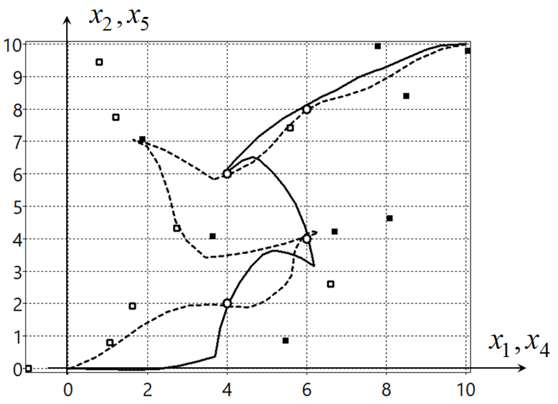
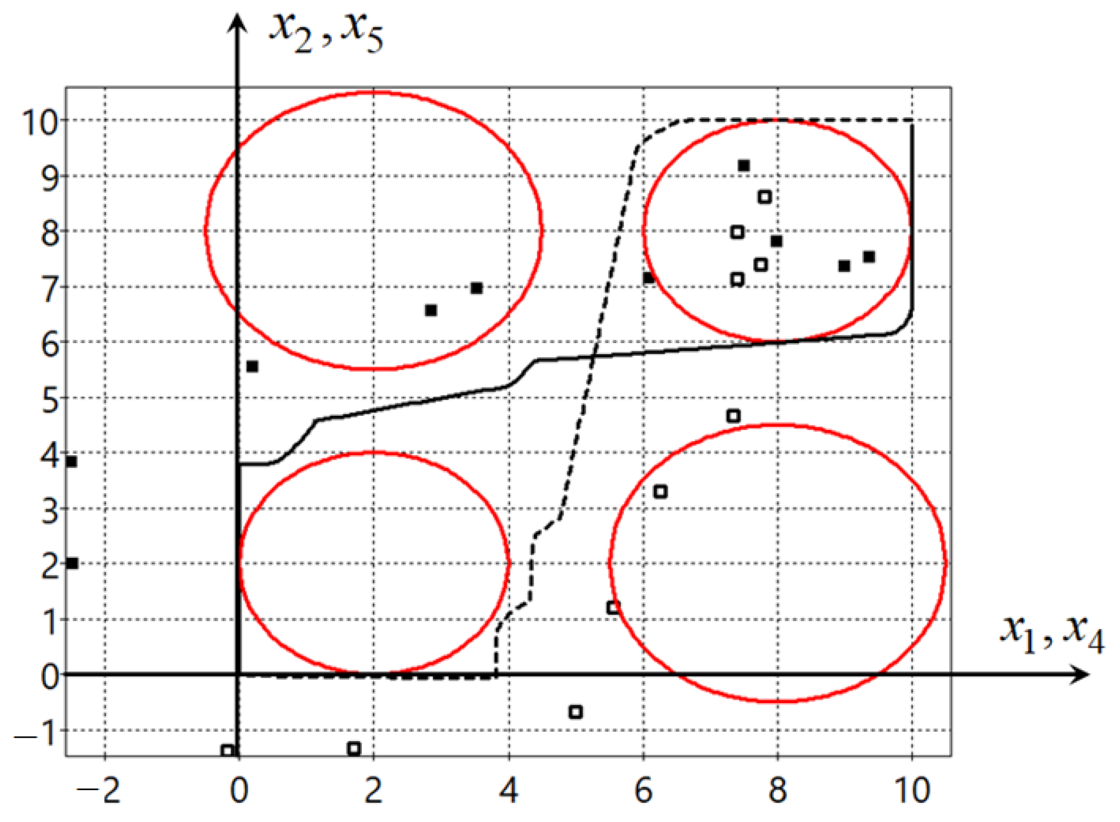
Optimal trajectories on horizontal plane for robots are presented in Figure 1.

In the Figure 1 the solid black line is a trajectory of the first robot, the dash line is a trajectory of the second robot, the small circles are the bottlenecks, the small black squares are the optimal control points (63) for the first robot, and the small white squares are the optimal control points (63) for the second robot. The optimal value of the functional (56) is $4.8347$.

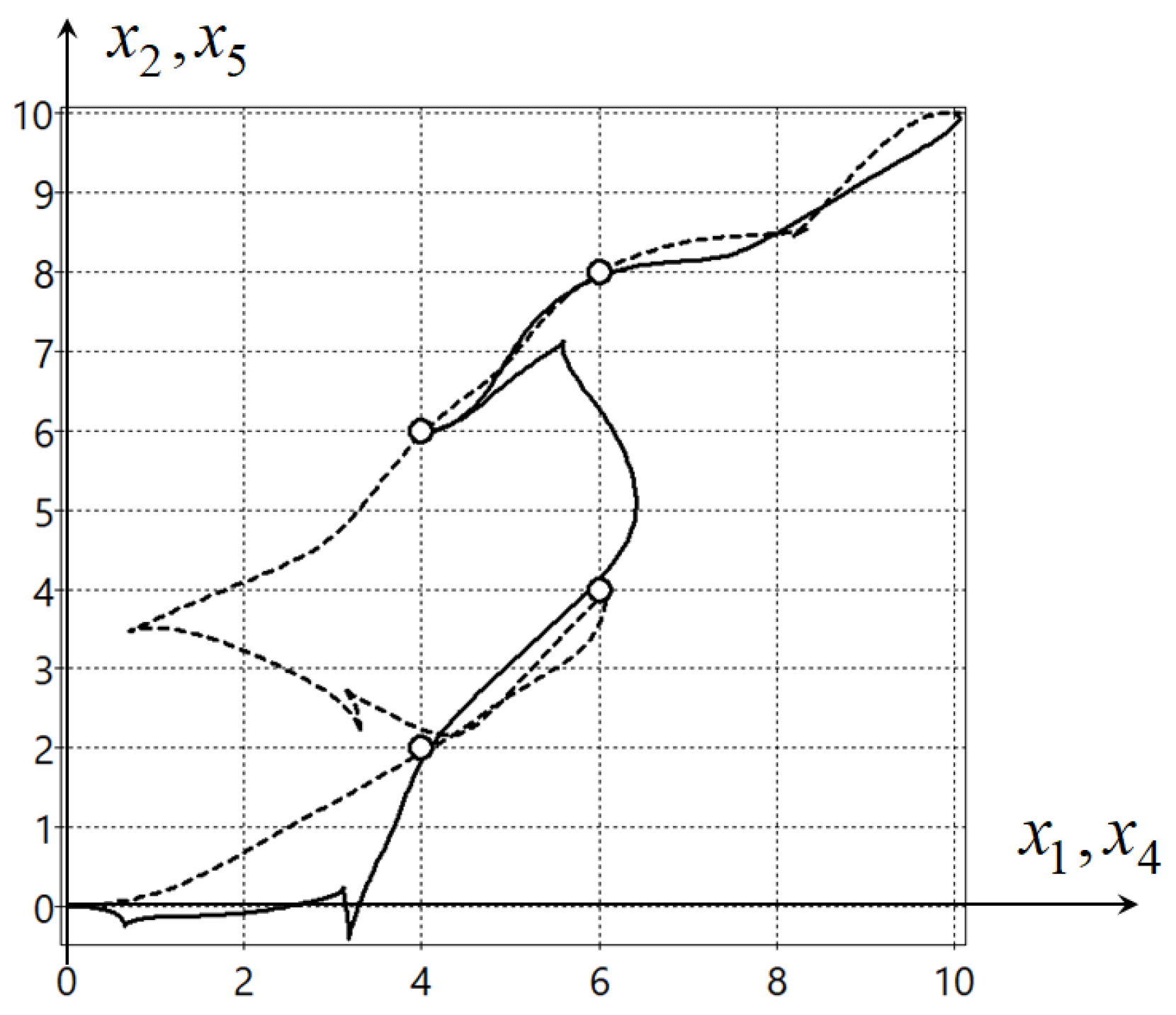
For comparison, the optimal control problem (52)–(60) was solved by the direct approach of optimal control. For this purpose, the time axis was divided on $\tilde{K}$ intervals. The control function is found in the form of the piece-wise linear function

$$u_j=\left\{\begin{array}{c}{u}_j^{+}=10,\mathrm{if}{\widehat{u}}_i>u_i^{+}\hfill \\ u_j^{-}=-10,\mathrm{if}{\widehat{u}}_i<u_i^{-}\hfill \\ {\widehat{u}}_j,\mathrm{otherwise}\hfill \end{array}\right.,j=1,2,3,4,$$

(64)

where

$${\widehat{u}}_j=(q_{i+(j-1)\tilde{K}+1}-q_{i+(j-1)\tilde{K}})\frac{t-(i-1)\widetilde{\Delta t}}{\widetilde{\Delta t}}+q_{i+(j-1)\tilde{K}}$$

(65)

where $j=1,2,3,4$, $j=1,\dots ,\tilde{K}$, $\tilde{\Delta }t$ is a time interval, $\tilde{\Delta }t=0.2$,

$$\tilde{K}=⌊\frac{t^{+}}{\tilde{\Delta }t}⌋=⌊\frac{4.8}{0.2}⌋=24.$$

(66)

In total, it is necessary to find 96 parameters, $\mathbf{q}={[q_1\dots q_{96}]}^T$. The problem was very difficult for many evolutionary algorithms. The most successful in solving this problem was the described hybrid evolutionary algorithm.

In the result, the following solution was obtained:

$$\begin{array}{ccc}\hfill \mathbf{q}& =& [3.6515-5.6155-5.8103-4.1722-3.1398-5.47110.0936\hfill \\ \hfill & & 6.61502.6432-8.8133-2.4498-18.5059-9.58960.1931\hfill \\ \hfill & & -5.5797-14.25169.53040.21810.6002-11.9435-12.2196\hfill \\ \hfill & & -0.0127-19.47128.85895.56958.48775.64590.7054-3.6582\hfill \\ \hfill & & -8.0966-0.6840-8.67747.7892-5.6366-5.3715-4.8317\hfill \\ \hfill & & -16.6047-19.8104-14.94747.67564.70009.7919-14.6483\hfill \\ \hfill & & -3.5860-3.1178-9.7188-16.2048-15.9328-1.31501.9570\hfill \\ \hfill & & -10.2673-0.5094-6.4163-4.9303-3.7649-6.3955\hfill \\ \hfill & & -5.8384-15.8273-9.2860-0.12179.0490-3.05430.8906\hfill \\ \hfill & & 7.634010.845910.24923.4207-10.6311-4.9477-3.4041\hfill \\ \hfill & & -13.6140-15.20294.8782-10.4763-10.58946.4966-4.2872\hfill \\ \hfill & & -12.7573-8.2174-0.8267-14.1822-1.6810-15.397312.1957\hfill \\ \hfill & & 15.469410.3573-12.78407.9684-6.393717.4171-6.62341.3378\hfill \\ \hfill & & {-8.2870-0.2343-18.0791-5.3433]}^T.\hfill \end{array}$$

(67)

The functional value is $4.8132$. The optimal trajectories on the horizontal plane are presented in Figure 2.

To analyze the received results, these optimal control functions were tested for the mathematical model with perturbations:

$$\begin{array}{ccc}\hfill {\dot{x}}_1& =& 0.5(u_1+u_2)cos\left(x_3\right)+\beta \xi \left(t\right),\hfill \\ \hfill {\dot{x}}_2& =& 0.5(u_1+u_2)sin\left(x_3\right)+\beta \xi \left(t\right),\hfill \\ \hfill {\dot{x}}_3& =& 0.5(u_1-u_2)+\beta \xi \left(t\right),\hfill \\ \hfill {\dot{x}}_4& =& 0.5(u_3+u_4)cos\left(x_6\right)+\beta \xi \left(t\right),\hfill \\ \hfill {\dot{x}}_5& =& 0.5(u_3+u_4)sin\left(x_6\right)+\beta \xi \left(t\right),\hfill \\ \hfill {\dot{x}}_6& =& 0.5(u_3-u_4)+\beta \xi \left(t\right),\hfill \end{array}$$

(68)

where $\xi \left(t\right)$ is a function that returns a random number from diapason $(-1;1)$ at every call, and $\beta$ is a constant value.

For the system (68), disturbances were also introduced into the initial conditions

$$x_{(}0)=x_i^0+{\beta }_0\xi ,i=1,\dots ,6,$$

(69)

where ${\beta }_0$ is a constant value. The results of the tests are presented in

Table 1. Functional values for perturbed control object model.

${\mathit{\beta }}_0$	$\mathit{\beta }$	${\mathit{J}}_3$	$\mathit{\sigma }\left({\mathit{J}}_3\right)$	${\mathit{J}}_4$	$\mathit{\sigma }\left({\mathit{J}}_4\right)$
0	0	$4.8347$	0	$4.8132$	0
0	$0.01$	$4.9999$	$0.1989$	$4.9267$	$0.1462$
0	$0.02$	$5.0868$	$0.288$	$5.1706$	$0.2559$
0	$0.05$	$5.3896$	$0.2087$	$6.1610$	$1.0704$
$0.01$	0	$5.2286$	$0.2053$	$6.5891$	$0.9445$
$0.02$	0	$5.4569$	$0.266$	$7.2853$	$1.6878$
$0.05$	0	$5.7369$	$0.6871$	$13.4286$	$3.5257$
$0.01$	$0.01$	$5.2365$	$0.2861$	$6.4381$	$0.9502$
$0.1$	0	$6.2945$	$0.7365$	$19.8192$	$8.0565$

. For every disturbance, 10 tests were performed. In Table 1, $J_3$ is an average functional value for synthesized control, $\sigma \left(J_3\right)$ is a standard deviation for values $J_3$, $J_4$ is an average functional value for direct control, and $\sigma \left(J_4\right)$ is a standard deviation for values $J_4$.

As the test results show, synthesized control is much less susceptible to perturbations of the mathematical model and the initial conditions than direct control. Direct optimal control is the most sensitive to disturbances of initial conditions. Even the smallest disturbances of the initial conditions make direct control unacceptable. The results show that the synthesized control obtains the compression property, and it is feasible in real systems.

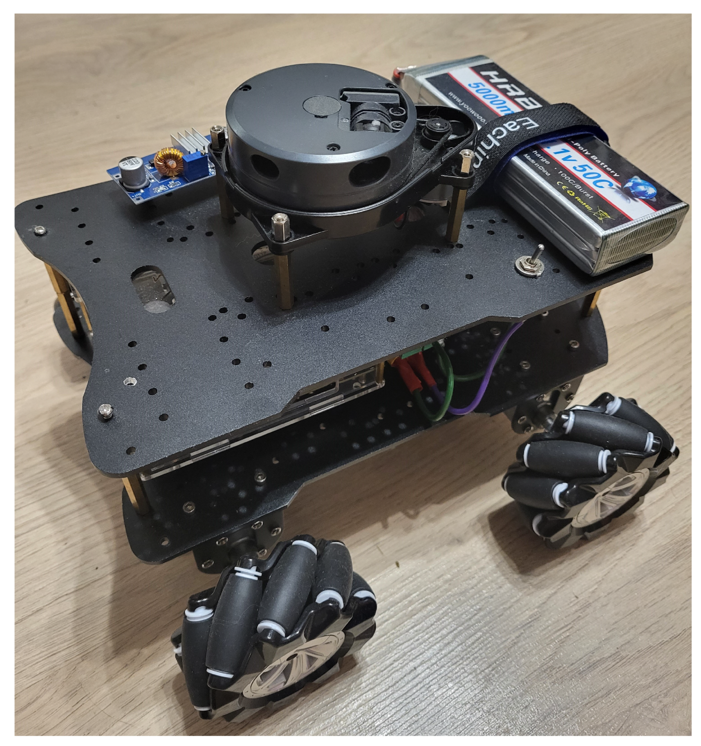
7.2. Synthesized Control for Omni-Mecanum-Wheeled Robot

A mecanum robot has special wheels that allow it to move under a direct angle to its direction of axis without any turns [51]. In Figure 3, an example of a mecanum robot is shown.

Consider the optimal control problem, where two identical mecanum robots have to swap their places in some area with obstacles and without collisions for a minimal amount of time.

The mathematical model of the control object is the following:

$$\begin{array}{ccc}\hfill {\dot{x}}_1& =& 0.25((u_1+u_4)(cos\left(x_3\right)+sin\left(x_3\right))+(u_2+u_3)(cos\left(x_3\right)-sin\left(x_3\right))),\hfill \\ \hfill {\dot{x}}_2& =& 0.25((u_1+u_4)(sin\left(x_3\right)-cos\left(x_3\right))+(u_2+u_3)(cos\left(x_3\right)+sin\left(x_3\right))),\hfill \\ \hfill {\dot{x}}_3& =& 0.25(-u_1+u_2-u_3+u_4)/(L_0+H_0),\hfill \\ \hfill {\dot{x}}_4& =& 0.25((u_5+u_8)(cos\left(x_6\right)+sin\left(x_6\right))+(u_6+u_7)(cos\left(x_6\right)-sin\left(x_6\right))),\hfill \\ \hfill {\dot{x}}_5& =& 0.25((u_5+u_8)(sin\left(x_6\right)-cos\left(x_6\right))+(u_6+u_7)(cos\left(x_6\right)+sin\left(x_6\right))),\hfill \\ \hfill {\dot{x}}_6& =& 0.25(-u_5+u_6-u_7+u_8)/(L_0+H_0),\hfill \end{array}$$

(70)

where $x_1$, $x_2$, and $x_3$ are the state vector coordinates of the first mecanum robot, $x_4$, $x_5$, and $x_6$ are the state vector coordinates of the second mecanum robot, $u_1$, $u_2$, $u_3$, and $u_4$ are components of the control vector of the first mecanum robot, $u_5$, $u_6$, $u_7$, and $u_8$ are components of the control vector of the first mecanum robot, and $L_0$ and $H_0$ are geometric parameters of the robots, $L_0=2$, $H_0=1$.

The control is restricted:

$$-10=u_i^{-}\le u_i\le u_i^{+}=10,i=1,\dots ,8,$$

(71)

where $u_i^{-}$ and $u_i^{+}$ are given lower and upper limits for values of control, respectively, $i=1,\dots ,8$.

The initial state is given:

$$\mathbf{x}\left(0\right)={\mathbf{x}}^0={\left[00010100\right]}^T.$$

(72)

The terminal state is given:

$$\mathbf{x}\left(t_f\right)={\mathbf{x}}^f={\left[10100000\right]}^T,$$

(73)

where $t_f$ is the time of achievement of the terminal state. It is determined by Equation (57) with ${\epsilon }_0=0.05$, $t^{+}=1.9$.

The quality criterion includes phase constraints and the accuracy of the terminal state achievement.

$$J=p_1\parallel {\mathbf{x}}^f-\mathbf{x}\left(t_f\right)\parallel +\sum _{i=1}^K{w}_i\underset{0}{\overset{t_f}{\int }}\vartheta \left({\varphi }_i\left(\mathbf{x}\right)\right)dt+p_2\underset{0}{\overset{t_f}{\int }}\vartheta \left(\chi \left(\mathbf{x}\right)\right)dt+t_f\to \underset{\mathbf{u}}{min},$$

(74)

where $p_1$ and $p_1$ are the penalty coefficient, where $p_1=3$ and $p_2=3$, $w_i$ is a weight coefficient, $i=1,\dots ,K$, $K=8$, $\vartheta \left(\alpha \right)$ is a Heaviside step function (59), and $\chi \left(\mathbf{x}\right)$ is determined by Equation (58):

$${\varphi }_i\left(\mathbf{x}\right)=r_i-\sqrt{\left(x_1\right)-x_{1,i}{)}^2+{(x_2-x_{2,i})}^2},i=1,2,3,4,$$

(75)

$${\varphi }_i\left(\mathbf{x}\right)=r_{i-4}-\sqrt{\left(x_4\right)-x_{1,i-4}{)}^2+{(x_5-x_{2,i-4})}^2},i=5,6,7,8,$$

(76)

$r_1=2$, $r_2=2.5$, $r_3=2.5$, $r_4=2$, $x_{1,1}=2$, $x_{2,1}=2$, $x_{1,2}=8$, $x_{2,2}=2$, $x_{1,3}=2$, $x_{2,3}=8$, $x_{1,4}=8$, $x_{2,4}=8$, $r_0=1$.

According to the synthesized method, initially, the feedback control synthesis problem is solved, such that the closed-loop control system is stable relative to some equilibrium point in the state space. For this purpose, again, the network operator method is used.

Since the robots are the same, we make the synthesis of the stabilization system for one robot, for example, the first robot.

In the result, the network operator method found the following control function:

$$u_i=\left\{\begin{array}{c}{u}_i^{+},\mathrm{if}{\tilde{u}}_i\ge u_i^{+}\hfill \\ u_i^{-},\mathrm{if}{\tilde{u}}_i\le u_i^{-}\hfill \\ {\tilde{u}}_i\mathrm{otherwise}\hfill \end{array}\right.,$$

(77)

where

$${\tilde{u}}_1=D+arctan\left(q_1{\Delta }_1\right),$$

(78)

$$\begin{array}{ccc}\hfill {\tilde{u}}_2& =& {\rho }_{19}\left({\tilde{u}}_1\right)+{\rho }_4\left(C\right)+{\rho }_{17}\left(B\right)+\mathrm{sgn}(q_2{\Delta }_2+\hfill \\ \hfill & & q_1{\Delta }_1+q_3\sqrt[3]{{\Delta }_3})+{\rho }_{18}\left(q_2{\Delta }_2\right)+q_1{\Delta }_1-{\left(q_1{\Delta }_1\right)}^3,\hfill \end{array}$$

(79)

$${\tilde{u}}_3={\tilde{u}}_2+C^3+A+arctan\left(q_1\right)-{(A+arctan\left(q_1\right))}^3+{\Delta }_2^{-1},$$

(80)

$$\begin{array}{ccc}\hfill {\tilde{u}}_4& =& sin\left({\tilde{u}}_3\right)+{\rho }_{16}\left({\tilde{u}}_2\right)+{(C+\sqrt[3]{{\Delta }_1})}^3+B+\hfill \\ \hfill & & \vartheta (q_2{\Delta }_2+q_1{\Delta }_1)+q_3\sqrt[3]{{\Delta }_3},\hfill \end{array}$$

(81)

$$A=\mathrm{sgn}(q_2{\Delta }_2+q_1{\Delta }_1+q_3\sqrt[3]{{\Delta }_3})+\vartheta (q_2{\Delta }_2+q_1{\Delta }_1),$$

$$B=A+arctan\left(q_1\right)+\mathrm{sgn}(q_2{\Delta }_2+q_1{\Delta }_1)+arctan\left(q_1{\Delta }_1\right),$$

$$\begin{array}{ccc}\hfill C& =& cos\left(B\right)+{\rho }_4(q_2{\Delta }_2+q_1{\Delta }_1)+{\rho }_{16}\left({\Delta }_1\right)+{\rho }_{19}(q_1{\Delta }_1+q_2{\Delta }_2)+exp\left(q_1{\Delta }_1\right),\hfill \end{array}$$

$$D=C+\sqrt[3]{{\Delta }_1}+C^3+{\rho }_B-A-arctan\left(q_1\right)+{\rho }_{16}\left(q_1{\Delta }_1\right),$$

${\Delta }_1=x_1^{*}-x_1$, ${\Delta }_2=x_2^{*}-x_2$, ${\Delta }_3=x_3^{*}-x_3$, $q_1=11.89282$, $q_2=10.15381$, $q_3=15.25903$,

$${\rho }_4\left(\alpha \right)=\mathrm{sgn}\left(\alpha \right)\sqrt{\left|\alpha \right|},{\rho }_{16}\left(\alpha \right)=\left\{\begin{array}{c}\alpha ,\mathrm{if}\left|\alpha \right|<1\hfill \\ \mathrm{sgn}\left(\alpha \right),\mathrm{otherwise}\hfill \end{array}\right.,$$

$${\rho }_{17}\left(\alpha \right)=\mathrm{sgn}\left(\alpha \right)ln\left(\right|\alpha |+1),{\rho }_{18}\left(\alpha \right)=\mathrm{sgn}\left(\alpha \right)(exp(\left|\alpha \right|)-1),$$

$${\rho }_{19}\left(\alpha \right)=\mathrm{sgn}\left(\alpha \right)exp(-|\alpha \left|\right).$$

For the second robot in the control function (77), it is necessary to replace $x_i$, $i=1,2,3$ with $x_i$, $i=4,5,6$, and $x_i^{*}$, $i=1,2,3$, with $x_i^{*}$$i=4,5,6$, respectively.

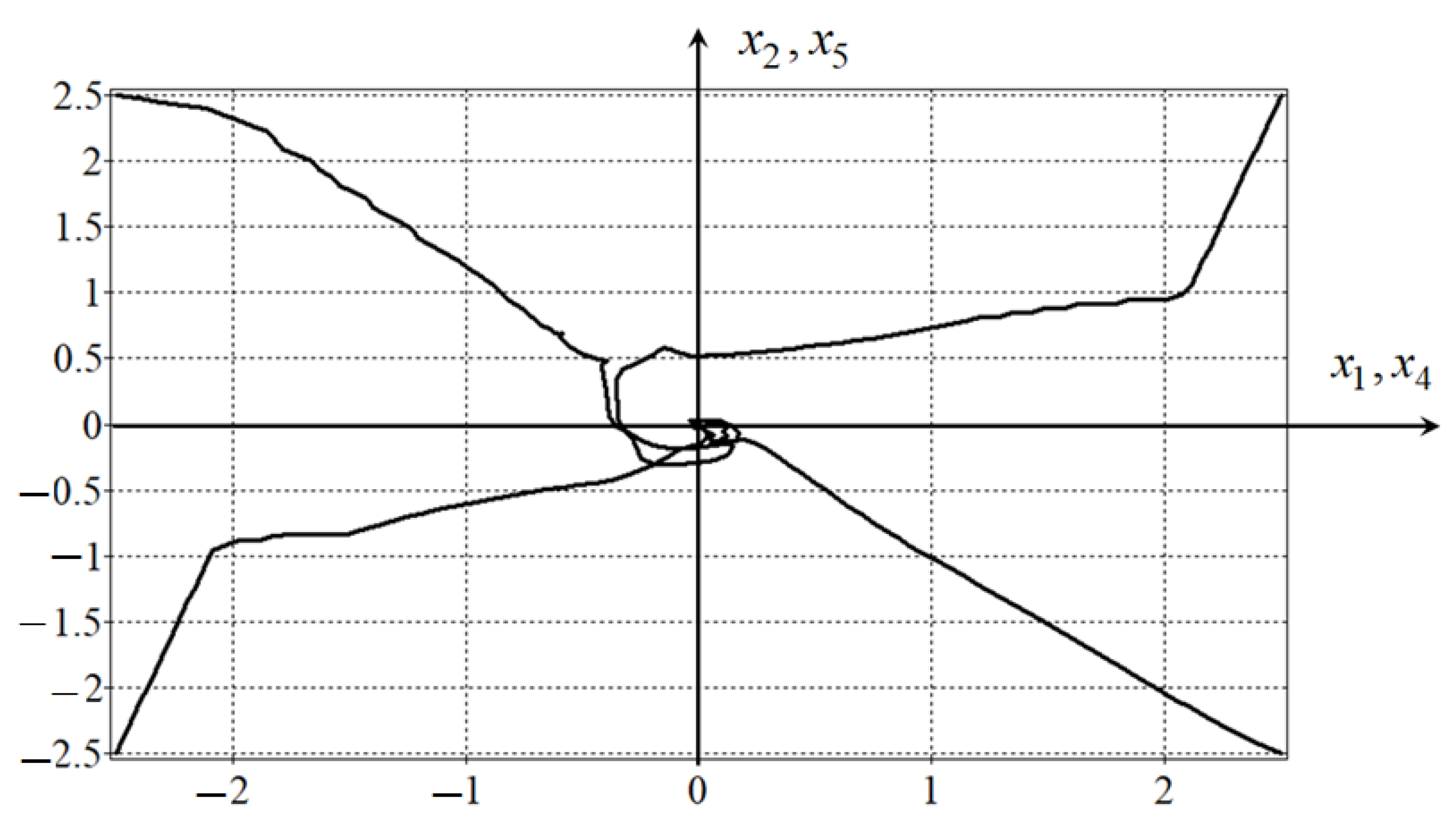
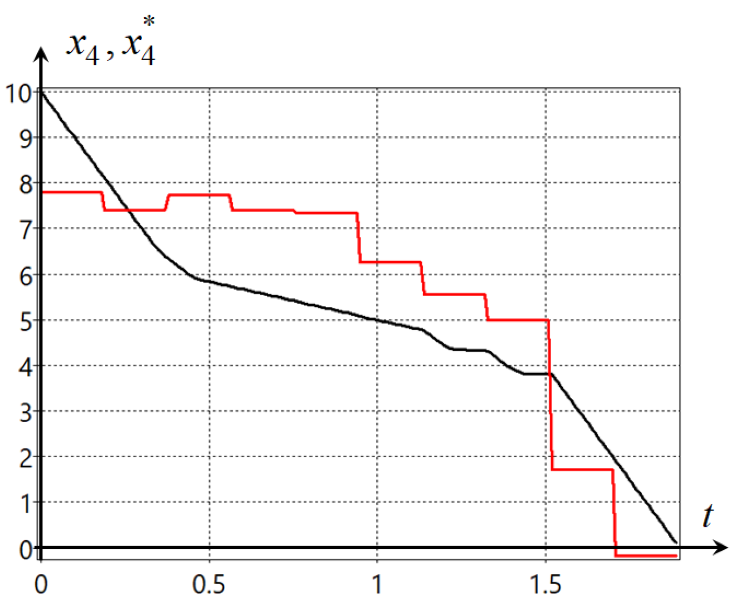
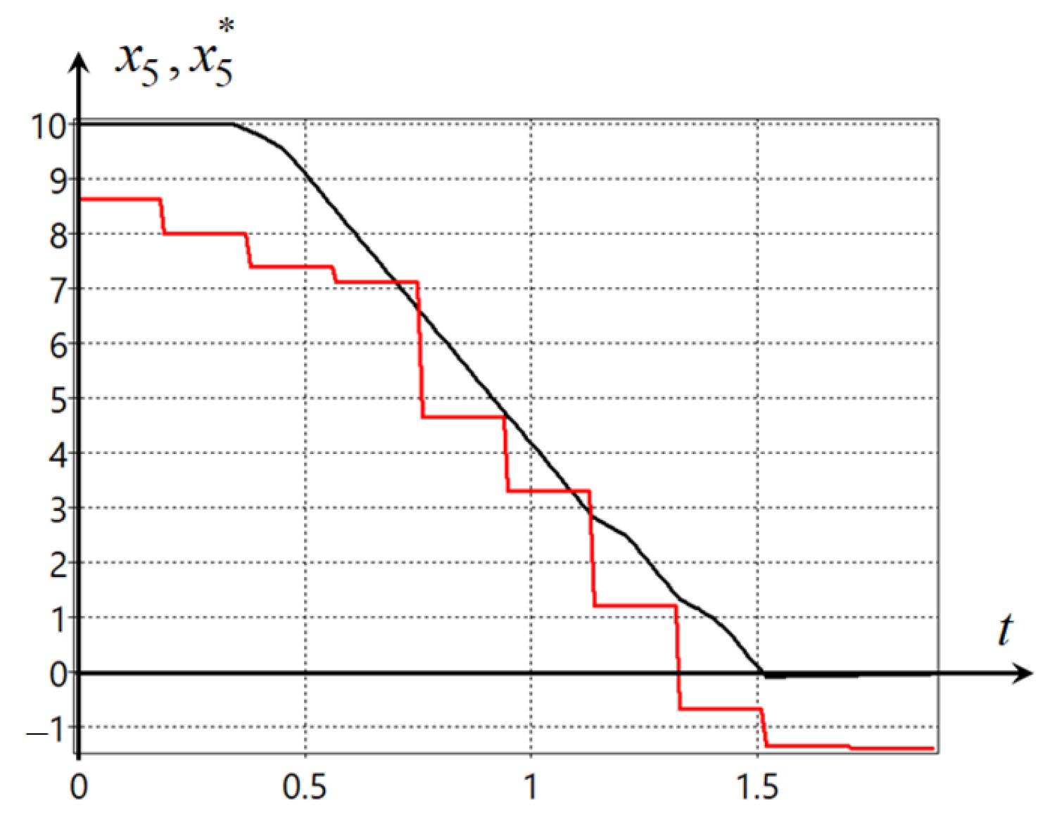
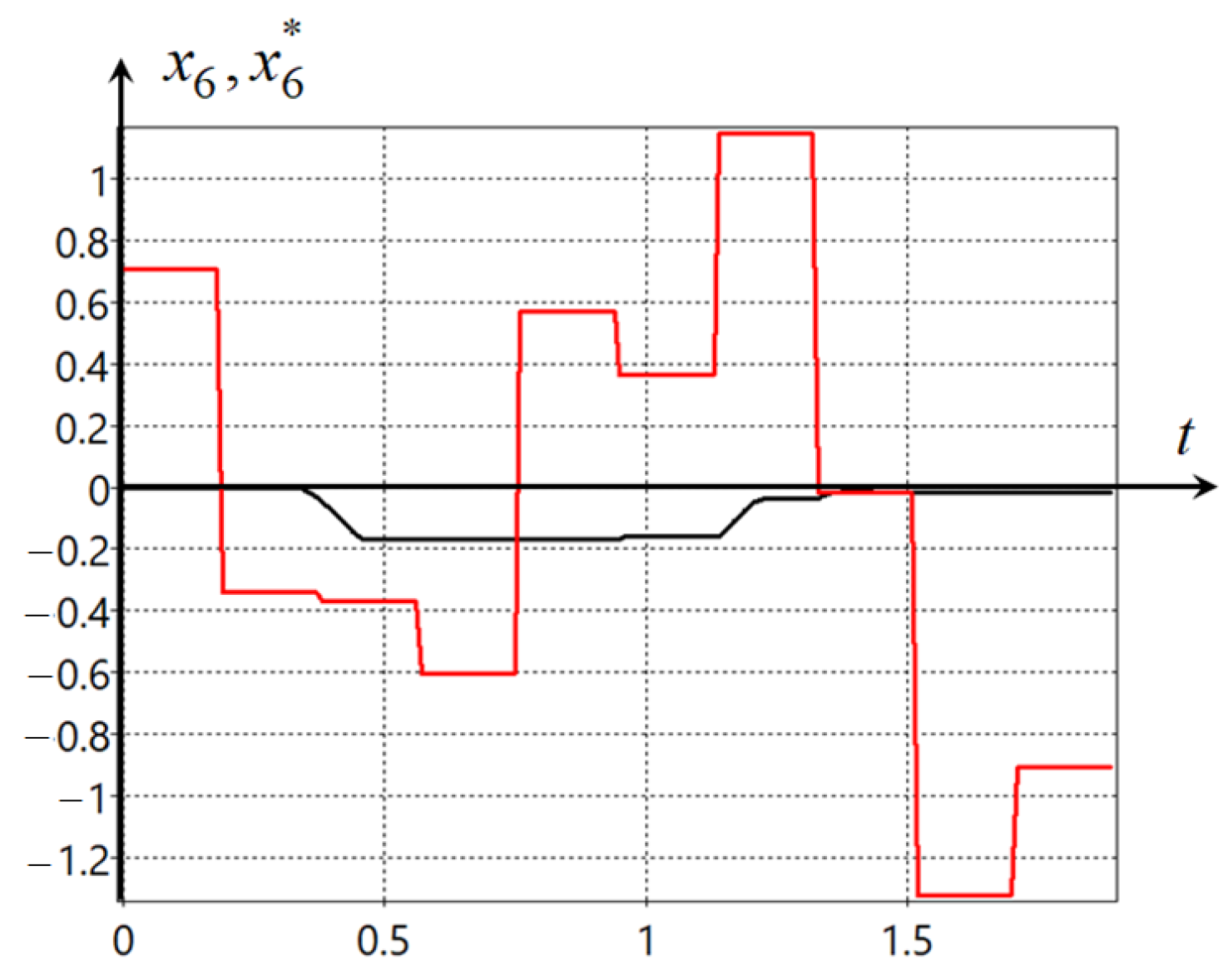
Plots of the trajectories of the robot movement from four initial states are presented in Figure 4.

On the second stage, the optimal control problem (70)–(74) is solved for the closed loop control system with the control function (77). A control on the second stage is vector ${\mathbf{x}}^{*}$, determining the position of the stable equilibrium point in the state space. For solving the optimal control problem, the time axis is divided on the intervals, and in each interval, a control function is approximated by a piece-wise constant function. The value of the interval is equal to $\Delta t=0.19$.

$$x_i^{*}=x_i\left(t_j\right)=q_{i+(j-1)6},$$

(82)

where $i=1,\dots ,6$, $t_j=(j-1)\Delta t$$j=1,\dots ,D$, D is the number of intervals,

$$D=\frac{t^{+}}{\Delta t}=\frac{1.9}{0.19}=10.$$

(83)

In total, it was necessary to find an optimal vector with $10·6=60$ parameters:

$$\mathbf{q}={[q_1\dots q_{60}]}^T.$$

For solving the problem, the hybrid evolutionary algorithm was applied. The values of the parameters were restricted:

$$\begin{array}{c}-2.5=q_1^{+}\le q_{1+3(k-1)}\le q_1^{-}=2.5\\ -2.5=q_2^{+}\le q_{2+3(k-1)}\le q_2^{-}=2.5\\ -5\pi /12=q_2^{+}\le q_{3+3(k-1)}\le q_2^{-}=5\pi /12\end{array},$$

(84)

where $k=1,\dots ,20$.

The following solution was obtained:

$$\begin{array}{c}\mathbf{q}=[-2.48622.00000.6231-2.1975-1.37990.7058-2.50001.9421\\ 1.2094-0.6933-2.0088-0.33780.19561.76430.63781.4052\\ -2.4611-0.32301.72452.00000.88721.6769-1.2832-0.4372\\ 0.56241.9987-1.16011.9452-1.88590.73571.68761.5024\\ 0.09971.1642-1.36780.53211.69451.99460.55800.7886\\ -1.60271.30901.17951.5385-1.07980.6781-1.99750.0204\\ -0.89391.0578-0.4106-2.1003-1.2544-1.3090-2.50001.0746\\ {-1.2216-2.0840-1.3344-0.8913]}^T.\end{array}$$

(85)

The optimal value of the functional (74) is $J=1.923$.

Optimal trajectories on the horizontal plane of two robots are presented in Figure 5. The solid line is the trajectory of the first robot, the dash line is the trajectory of the second robot, the red circles are the phase constraints, the black small squares are projections of control ${\mathbf{x}}^{*}$ on the horizontal plane for the first robot, and the white small squares are projections of control ${\mathbf{x}}^{*}$ on the horizontal plane for the second robot.

Figure 5 shows very clearly, as in the previous example with bottlenecks, that the equilibrium points are located not on the trajectory of the robot, as is done with conventional stabilization, but outside the trajectory. By placing points on the trajectory, we can lose quality because when approaching the equilibrium point, the robot must slow down. Such an optimal arrangement of points ensures the optimal value of the functional.

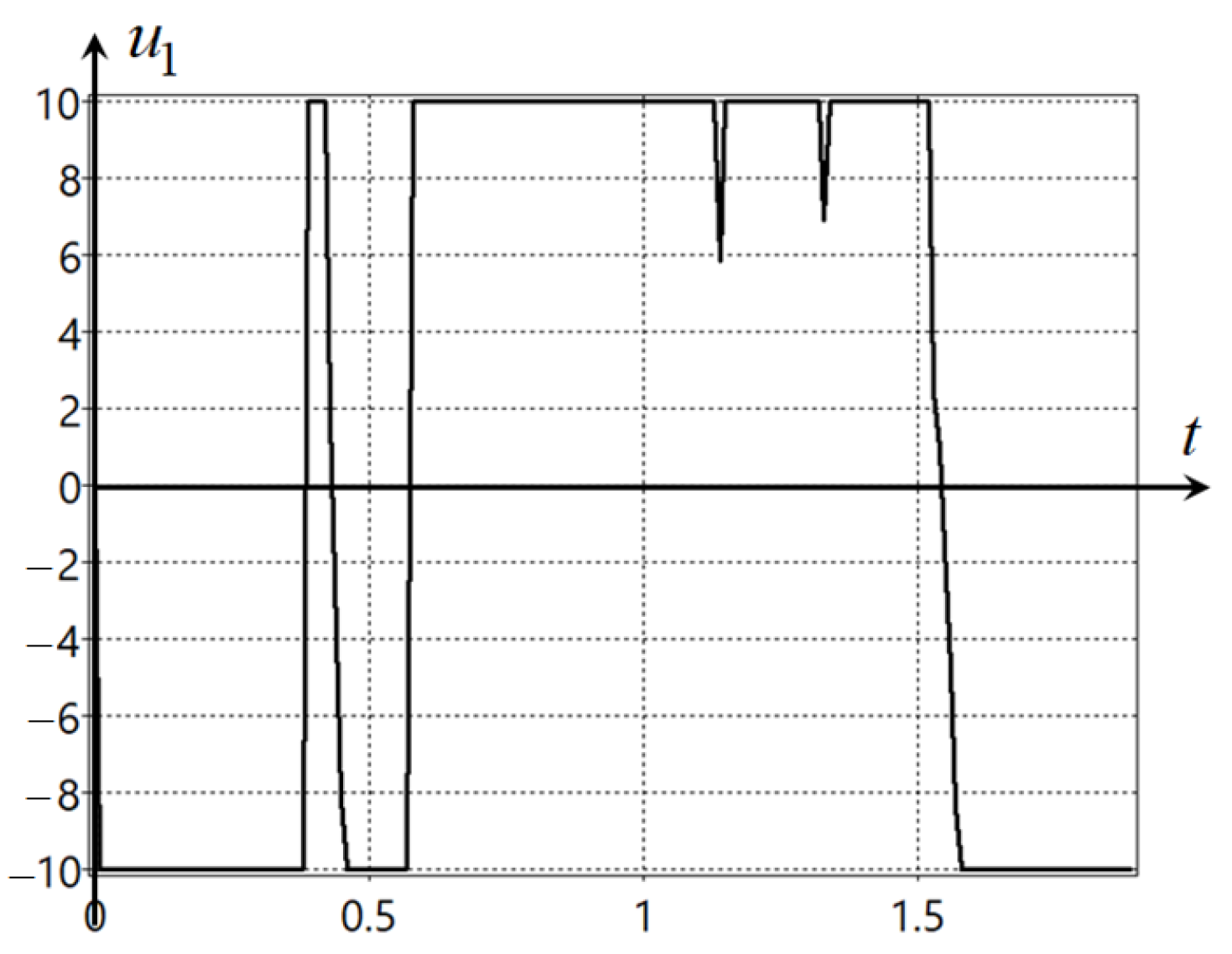
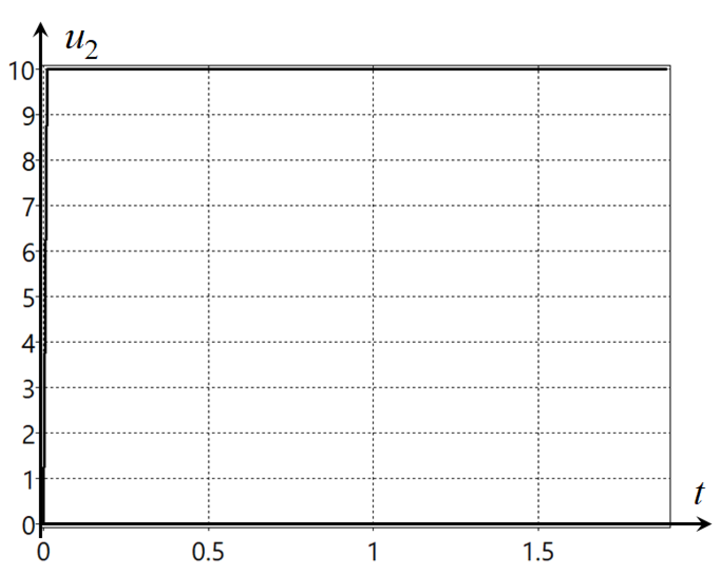
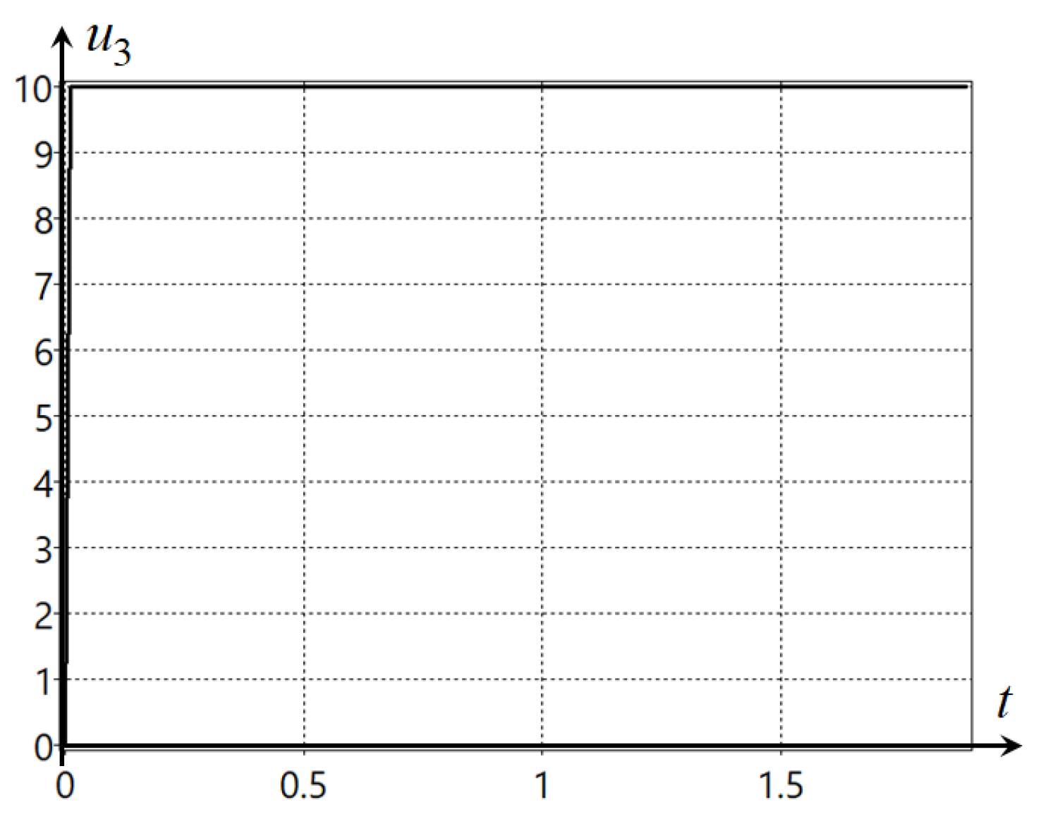
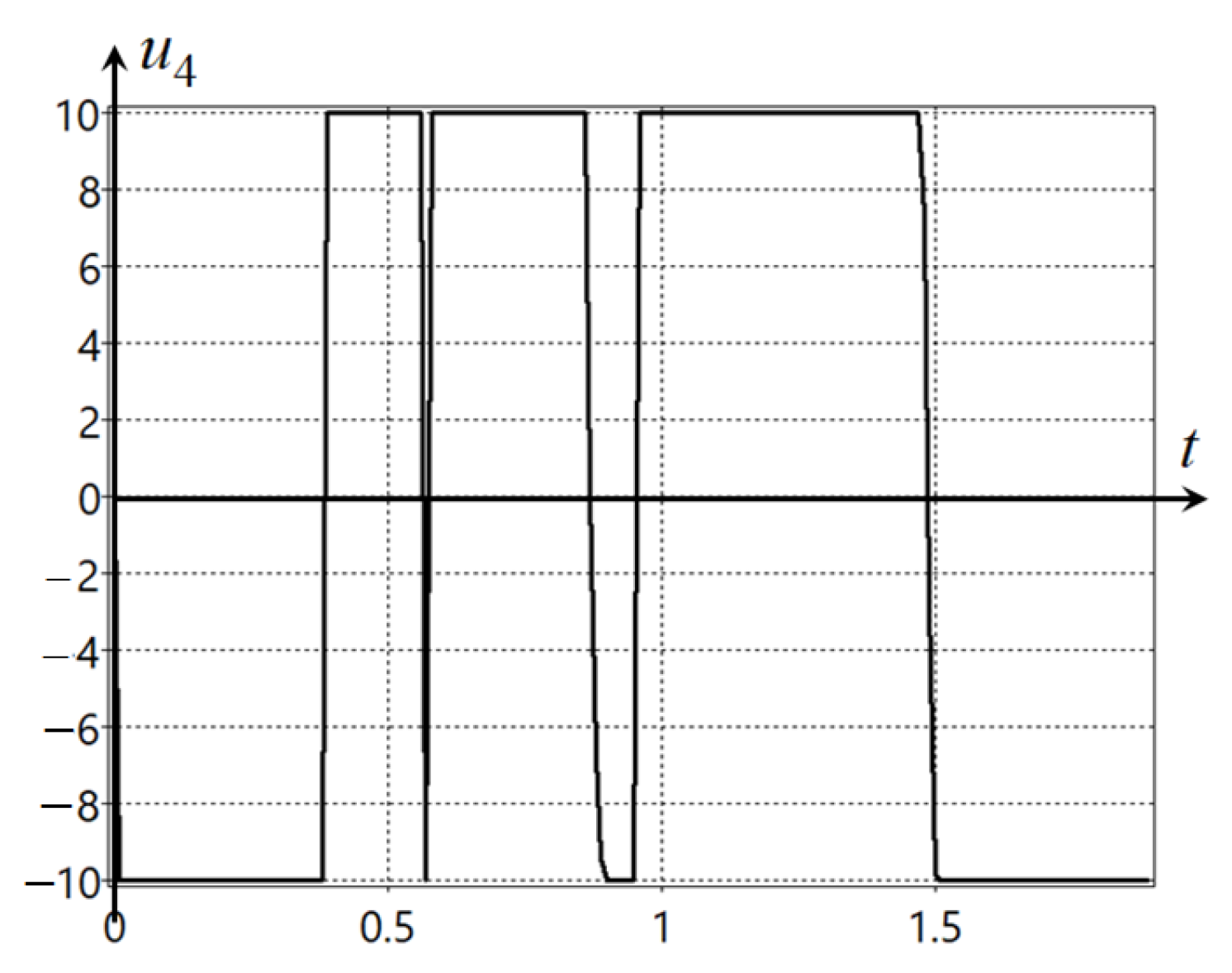
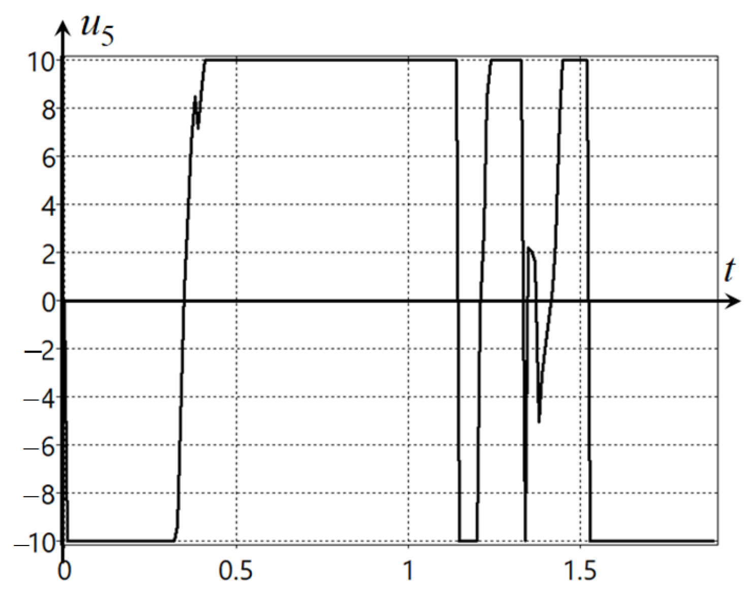
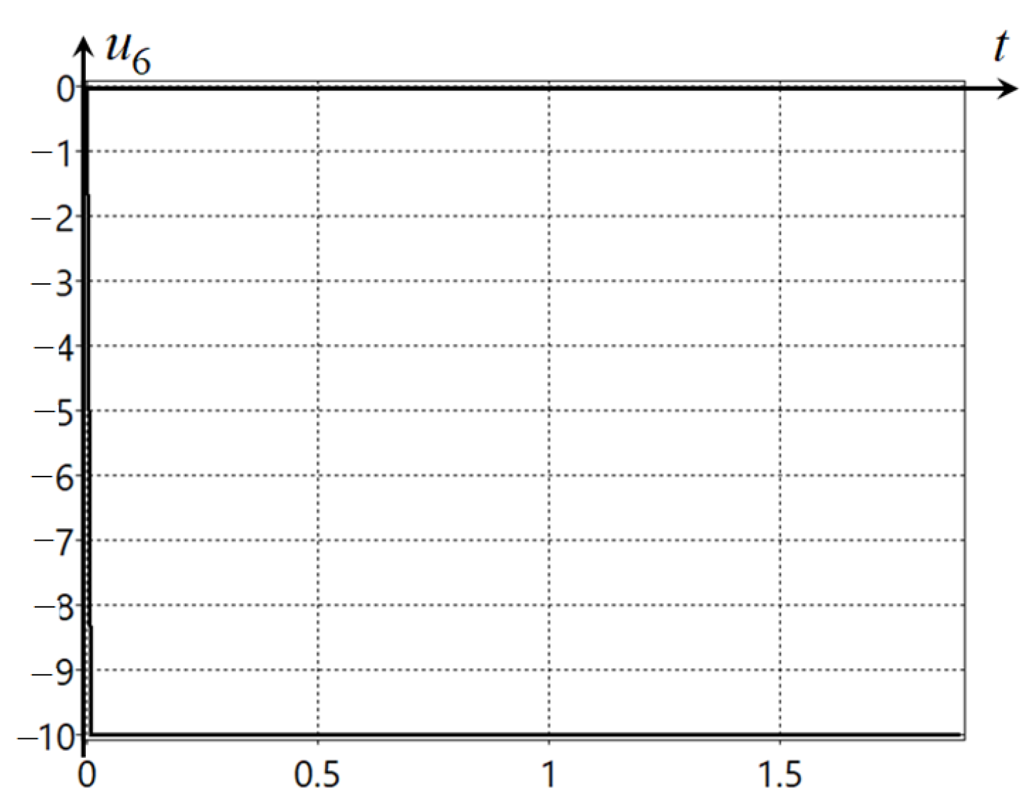
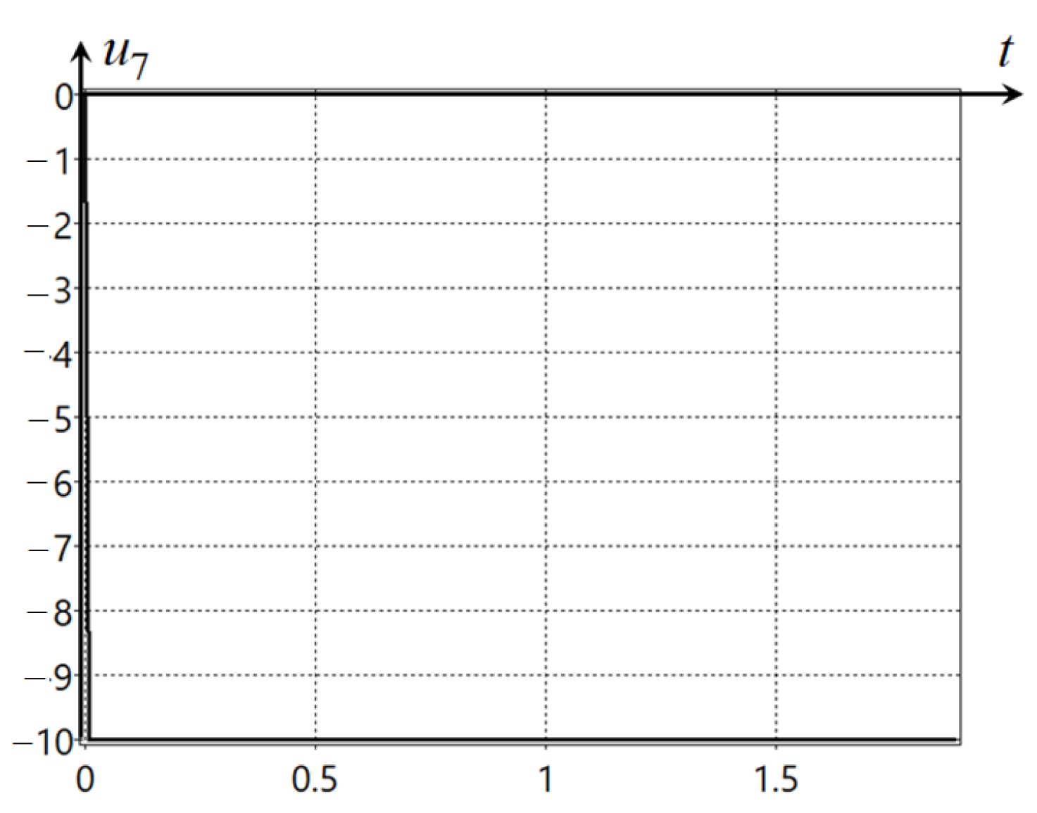
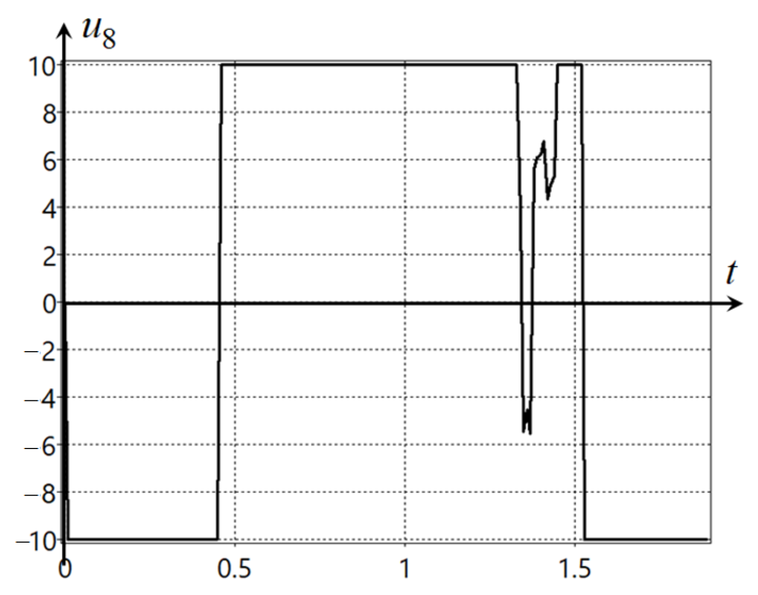
In this example, we would like to note the following. It occurs that two components of the control vector are enough to control the mecanum robot. The other two components have limit values and do not change during the control process. This can be seen in the additional control plots presented in Appendix C. However, indeed, we noted that in the mathematical model of the mecanum robot (70), the control was redundant, $m>n$. So, the computer itself found a solution for how to proceed in this case, and in the solution found, the two components of control, in fact, do not participate in the search for the optimal solution. This is one of the more successful demonstrations of intelligent machine automation of the process of creating control systems.

8. Discussion

In this work, we are laying the theoretical foundations of machine learning control. The main feature is that the machine proof of various properties is implemented experimentally basing on examples. In particular, this is what happens in neural networks, when experiments are carried out on a test sample to check whether the system achieves certain properties. We formulate several machine properties in the control system design. In the future, the proposed formal descriptions can be developed, new properties of systems can be considered, and quantitative probabilistic estimates can be given based on positive test results.

An important result of the work is the expansion of the formulation of the optimal control problem and the introduction of additional requirements for the required control. Ensuring the introduced conditions additionally requires the introduction of feedback. The paper presents the approach of synthesized optimal control, which allows implementing optimal control systems, taking into account the introduced additional requirement. In this case, other approaches can be considered and proposed.

9. Conclusions

A general machine learning approach for the automatic design of feedback control systems for any dynamical nonlinear control objects is considered. The main perspective is the machine-automated development of control systems. According to this trend, the control system is obtained as a result of a machine solution of some formal mathematical control problem and it is to be implemented in the real object directly.

Since the control system is created by machine learning, the paper formulates a machine check of all the properties required from the control system. Mathematical statements of control problems and some theoretical justifications for solution of these problems by machine methods are presented. The paper introduces and discusses such notions as machine learning control, stability, optimality and feasibility of machine-made control systems. In this regard, substantiations are introduced for the machine learning feedback control approach based on symbolic regression and evolutionary algorithms.

Thus, the feedback control design is generalized and automated with a generic approach applicable to any nonlinear models, including machine-learning-identified models. It is shown that with this approach, the computer is able to propose interesting outstanding solutions, which sometimes an engineer cannot even suppose.

There is another feature in the proposed approach that can be developed in a good direction. It is possible to control an object by controlling the position of the equilibrium point both offline under predetermined operating conditions, and online, when the positions of the points can be optimally planned for some short term and then adjusted according to the situation. This is one more direction for further research and application of the presented approach.