A New ϵ-Adaptive Algorithm for Improving Weighted Compact Nonlinear Scheme with Applications

Abstract

To improve the resolution and accuracy of the high-order weighted compact nonlinear scheme (WCNS), a new $ϵ$-adaptive algorithm based on local smoothness indicators is proposed. The new algorithm introduces a high-order global smoothness indicator to adjust the value of $ϵ$ according to the local flow characteristics. Specifically, the algorithm increases $ϵ$ in smooth regions, which can help cover up the disparity in smoothness indicators of sub-stencils and make the nonlinear scheme approach the background linear scheme. As a result, optimal order accuracy can be achieved in smooth regions, including critical points. While near discontinuities, the algorithm decreases $ϵ$, thereby strengthening the stencil selection mechanism and further attenuating spurious oscillations. Meanwhile, the new algorithm makes nonlinear schemes scale-invariant of flow variables. The results of approximate dispersion relation (ADR) show that the new algorithm can greatly reduce spectral errors of nonlinear schemes in the medium and low wavenumber range without inducing instability. Numerical results indicate that the new algorithm can significantly improve resolution of small-scale structures and suppress numerical oscillations near discontinuities with only a minor increment in computational cost.

1. Introduction

High-order accurate and high-resolution numerical schemes have always been the forefront of research in the field of CFD. In the past few decades, high-order shock-capturing schemes have flourished, laying the foundation for the refined simulation of multi-scale complex flow phenomena with discontinuities. The weighted essentially non-oscillatory (WENO) scheme is one of the most widely used shock-capturing schemes due to its balanced performance for resolving both small-scale flow structures and discontinuities. Harten [1] first put forward the essential non-oscillatory (ENO) scheme, then Liu et al. [2] constructed the famous weighted ENO (WENO) scheme by introducing the nonlinear weighting technique. The WENO scheme has higher order accuracy and higher resolution while retaining the essential non-oscillatory property. Later, Jiang and Shu [3] made important improvements to the nonlinear weights, formulating the classic WENO-JS, which promoted extensive research on the WENO scheme. They proposed a new local smoothness indicator to help the WENO scheme achieve optimal order accuracy on the original stencil.

However, the WENO-JS scheme can be dissipative for fine-scale simulations and suffers a loss of accuracy at critical points in smooth regions. Henrick et al. [4] found the reason for this and proposed the mapped WENO scheme (WENO-M), which recovers optimal order accuracy at first-order critical points. Compared with the WENO-JS scheme, the WENO-M scheme has higher resolution; however, the computational cost is increased by about 25%. Later, Borges et al. [5] put forward an ingenious weight function by introducing a high-order global smoothness indicator, and established the WENO-Z scheme with lower dissipation and higher resolution. The advantage of the WENO-Z scheme is that it can ensure optimal order accuracy at first-order critical points at the expense of minorly increased computational cost. Since then, a series of improved and optimized schemes [6,7,8,9,10,11] were developed based on these two representative works. Meanwhile, some researchers [4,6,12,13,14,15,16,17,18] paid attention to the small quantity $ϵ$ in weight functions to further improve the performance of schemes.

The small quantity $ϵ$ in the nonlinear weight function was originally introduced to avoid the denominator becoming zero. To capture the shock stably, $ϵ$ is generally taken as a small constant. With further research, it was found that the value of $ϵ$ can greatly influence the convergence speed, the accuracy at critical points, and the numerical oscillations near discontinuities. Henrick et al. [4] pointed out that the convergence order of the WENO-JS scheme depends on $ϵ$ and grid spacing, and there are numerical oscillations of order ${ϵ}^2$ near discontinuities. Shen et al. [12] found that the weights of the original WENO-JS scheme oscillate even in smooth regions, and increasing $ϵ$ to ${10}^{-2}$ can significantly suppress oscillations of nonlinear weights while maintaining the shock-capturing capability. However, it only works for subsonic and transonic flows. For supersonic and hypersonic flows, increasing $ϵ$ may cause serious numerical oscillations near strong shock waves, and even lead to calculation failure. Therefore, setting $ϵ$ as a constant has great limitations.

To avoid the empirical selection of $ϵ$, and to diminish the influence of $ϵ$ on the accuracy at critical points and the numerical oscillations near discontinuities, some adaptive algorithms for $ϵ$ have been developed. Yamaleev and Carpenter [13] set $ϵ$ as a power-function of grid spacing, which can achieve optimal order accuracy regardless of critical points. Hu and Adams [14] set $ϵ$ as ${10}^{-8}{h}^2$ in the scale separation study of implicit large eddy simulation, which yielded more accurate results. Don and Borges [6] derived the accurate conditions for the power-function to make WENO-JS and WENO-Z schemes achieve optimal order accuracy at high-order critical points. Aràndiga et al. [15] pointed out that the method proposed by Yamaleev and Carpenter [13] has only first-order accuracy near discontinuities, which is reflected as serious numerical oscillations in the numerical tests. They modified the weight function to improve the order accuracy near discontinuities and alleviate numerical oscillations. Although these $ϵ$-adaptive algorithms based on the power-function of grid spacing can theoretically ensure optimal order accuracy regardless of critical points, they will also aggravate numerical oscillations near high-order critical points and discontinuities and affect the convergence of calculation with limited number of grid points.

Another representative class of adaptive algorithms is constructed based on the smoothness indicators of sub-stencils. Peer et al. [16] proposed an adaptive $ϵ$ that depends on the difference of smoothness indicators. The algorithm adopts ${10}^{-6}$ in smooth regions and switches to a smaller value near discontinuities, which further suppresses the numerical oscillations of the WENO-JS scheme near discontinuities. Based on the global smoothness indicator, Jia et al. [17] designed a piecewise function to calculate $ϵ$ to reduce nonlinear errors in smooth regions and suppress numerical oscillations near discontinuities. However, this adaptive algorithm contains four free empirical parameters to be manually adjusted in practical computations, which hinders the application and popularization of the algorithm. Recently, Zheng et al. [18] proposed a parameter-free $ϵ$-adaptive algorithm, which can help reduce numerical dissipation in smooth regions, suppress numerical oscillations near discontinuities, and lessen susceptibility to flux functions and interpolation variables. Unfortunately, these adaptive algorithms will inevitably lose accuracy near critical points due to the large relative disparity in smoothness indicators of sub-stencils.

In this paper, a new simple $ϵ$-adaptive algorithm based on smoothness indicators of sub-stencils is proposed to address the issues of accuracy at critical points and nonlinear error in smooth regions. The wavenumber analysis and numerical results show that compared with the existing adaptive algorithms, the nonlinear scheme with the new adaptive algorithm has higher resolution and lower dissipation and dispersion errors, further suppresses numerical oscillations near discontinuities while maintaining optimal order accuracy at critical points, and has a lower computational cost. The present work is based on the weighted compact nonlinear scheme (WCNS) [19,20], which adopts the nonlinear weighting technique of WENO and has been widely applied to numerical simulations of various complex flows [21,22,23,24,25].

The organization of this paper is as follows. Section 2 briefly introduces the fifth-order WCNS scheme, followed by the development of a new $ϵ$-adaptive algorithm, then the accuracy at critical points and the spectral properties are discussed. Section 3 presents a series of benchmark tests to validate the new adaptive algorithm. Finally, conclusions are given in Section 4.

2. Numerical Methods

2.1. Difference Scheme

For simplicity, we consider the following one-dimensional hyperbolic conservation law

$$\begin{array}{c}\hfill \frac{\partial u}{\partial t}+\frac{\partial f\left(u\right)}{\partial x}=0,x\in [a,b],t\in [0,\infty )\end{array}$$

(1)

where $u(x,t)$ is the conserved quantity, and $f\left(u\right)$ is the flux. Consider a uniform mesh defined by $x_j=jh(j=0,1,...,N)$, where $h=(b-a)/N$, then the semi-discrete form of Equation (1) yields

$$\begin{array}{c}\hfill \frac{d{u}_j\left(t\right)}{dt}=-F_j^{\prime }\end{array}$$

(2)

where $u_j\left(t\right)$ and $F_j^{\prime }$ are numerical approximations of $u(x_j,t)$ and $\frac{\partial f}{\partial x}{|}_{x_j}$, respectively.

The original WCNS scheme mostly used compact difference schemes to compute $F_j^{\prime }$. Later, it was found that the form of the difference schemes, explicit or compact, has few effects on spectral properties and numerical results. Therefore, the more efficient and simple explicit difference schemes are recommended [24,26]. In this paper, we use the sixth-order explicit central difference scheme to compute $F_j^{\prime }$

$$\begin{array}{c}\hfill F_j^{\prime }=\frac{75}{64h}\left({\widehat{F}}_{j+1/2}-{\widehat{F}}_{j-1/2}\right)-\frac{25}{384h}\left({\widehat{F}}_{j+3/2}-{\widehat{F}}_{j-3/2}\right)+\frac{3}{640h}\left({\widehat{F}}_{j+5/2}-{\widehat{F}}_{j-5/2}\right)\end{array}$$

(3)

where ${\widehat{F}}_{j\pm k/2}=\widehat{F}({\tilde{u}}_{j\pm k/2}^{\mathrm{L}},{\tilde{u}}_{j\pm k/2}^{\mathrm{R}})(k=1,3,5)$ are numerical fluxes at cell-edges $j\pm k/2$, which can be obtained with different types of convective flux functions, such as Steger-Warming and Roe splitting schemes. ${{\tilde{u}}^{\mathrm{L}}}_{j+1/2}$ and ${{\tilde{u}}^{\mathrm{R}}}_{j+1/2}$ are interpolated variables at the cell-edge. Assuming that numerical fluxes in Equation (3) are equal to exact fluxes, e.g.,

$$\begin{array}{c}\hfill {\widehat{F}}_{j+1/2}=f_{j+1/2}=f_j+{\displaystyle \sum _{n=1}^{\infty }}{f_j}^{\left(n\right)}\frac{{(h/2)}^n}{n!}\end{array}$$

(4)

Then, by replacing numerical fluxes in Equation (3) with these Taylor series expansions, we have

$$\begin{array}{c}\hfill F_j^{\prime }=f_j^{\prime }+\frac{5f_j^{\left(7\right)}}{7168}{h}^6+O\left(h^8\right)\end{array}$$

(5)

Thus, Equation (3) with exact cell-edge fluxes, gives an approximation of $f_j^{\prime }$ with sixth-order accuracy.

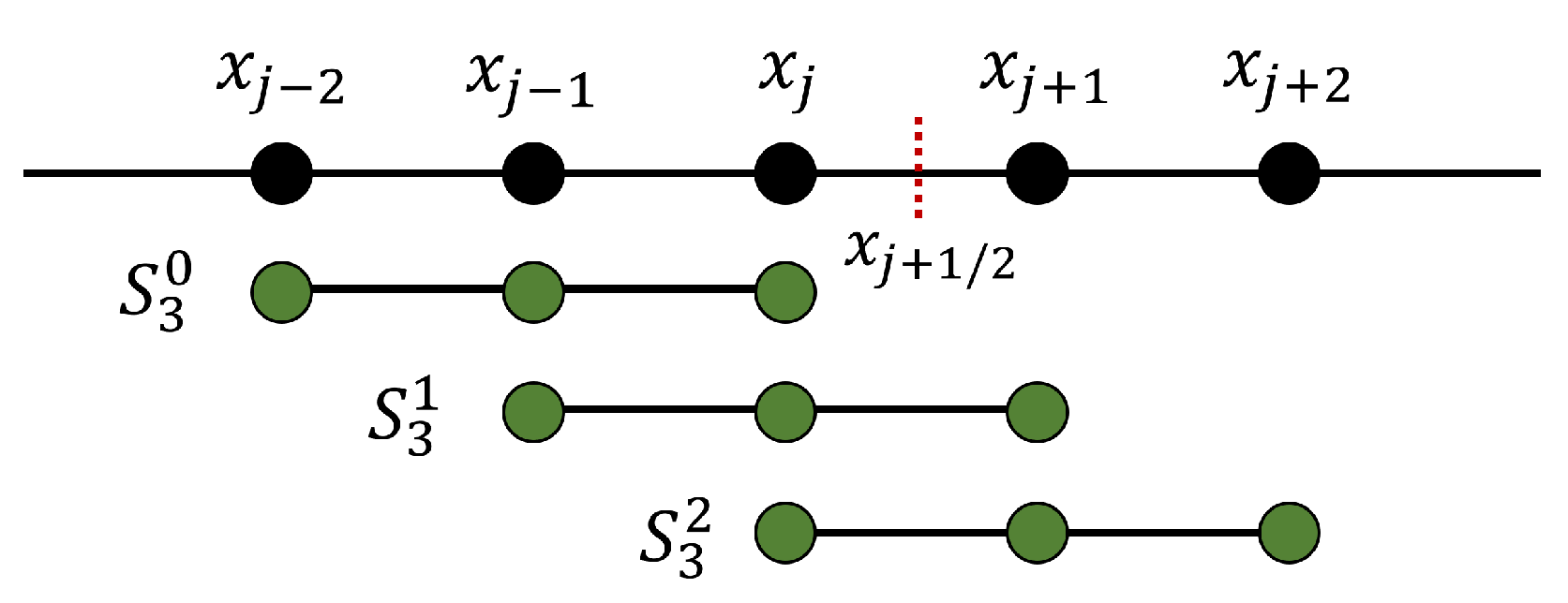
2.2. Interpolation Scheme

The interpolation scheme dominates the resolution characteristics of the WCNS scheme [20,24,26], which is briefly introduced in this section. Only interpolation of ${{\tilde{u}}^{\mathrm{L}}}_{j+1/2}$ is considered here and the superscript L is removed for simplicity. The interpolation of ${{\tilde{u}}^{\mathrm{R}}}_{j+1/2}$ has a mirror form with ${{\tilde{u}}^{\mathrm{L}}}_{j+1/2}$ and is not shown to save space.

As shown in Figure 1, the fifth-order WCNS scheme conducts nonlinear interpolation of ${\tilde{u}}_{j+1/2}$ on a five-point stencil, denoted by $S_5=\left\{x_{j-2},x_{j-1},x_j,x_{j+1},x_{j+2}\right\}$. The five-point stencil is divided into three three-point sub-stencils, denoted by $S_3^k=\left\{x_{j+k-2},x_{j+k-1},x_{j+k}\right\}$$(k=0,1,2)$. On each three-point sub-stencil $S_3^k$, a quadratic interpolation polynomial $p_k\left(x\right)$ can be obtained as follows

$$\begin{array}{cc}\hfill & p_0\left(x\right)=\frac{u_{j-2}-2u_{j-1}+u_j}{2}{\left(\frac{x-x_j}{h}\right)}^2+\frac{u_{j-2}-4u_{j-1}+3u_j}{2}\left(\frac{x-x_j}{h}\right)+u_j\hfill \\ \hfill & p_1\left(x\right)=\frac{u_{j-1}-2u_j+u_{j+1}}{2}{\left(\frac{x-x_j}{h}\right)}^2+\frac{u_{j+1}-u_{j-1}}{2}\left(\frac{x-x_j}{h}\right)+u_j\hfill \\ \hfill & p_2\left(x\right)=\frac{u_j-2u_{j+1}+u_{j+2}}{2}{\left(\frac{x-x_j}{h}\right)}^2+\frac{-3u_j+4u_{j+1}-u_{j+2}}{2}\left(\frac{x-x_j}{h}\right)+u_j\hfill \end{array}$$

(6)

Then the third-order linear interpolations at $x_{j+1/2}$ are

$$\begin{array}{cc}\hfill & {\tilde{u}}_{j+1/2}^0=p_0\left(x_{j+1/2}\right)=\frac{1}{8}\left(3u_{j-2}-10u_{j-1}+15u_j\right)\hfill \\ \hfill & {\tilde{u}}_{j+1/2}^1=p_1\left(x_{j+1/2}\right)=\frac{1}{8}\left(-u_{j-1}+6u_j+3u_{j+1}\right)\hfill \\ \hfill & {\tilde{u}}_{j+1/2}^2=p_2\left(x_{j+1/2}\right)=\frac{1}{8}\left(3u_j+6u_{j+1}-u_{j+2}\right)\hfill \end{array}$$

(7)

Taylor series expansion of Equation (7) yields

$$\begin{array}{cc}\hfill & {\tilde{u}}_{j+1/2}^0=u_{j+1/2}-\frac{5u_{j+1/2}^{\left(3\right)}}{16}{h}^3+O\left(h^4\right)\hfill \\ \hfill & {\tilde{u}}_{j+1/2}^1=u_{j+1/2}+\frac{u_{j+1/2}^{\left(3\right)}}{16}{h}^3+O\left(h^4\right)\hfill \\ \hfill & {\tilde{u}}_{j+1/2}^2=u_{j+1/2}-\frac{u_{j+1/2}^{\left(3\right)}}{16}{h}^3+O\left(h^4\right)\hfill \end{array}$$

(8)

To capture discontinuities stably, a nonlinear combination of these third-order linear interpolations is performed

$$\begin{array}{c}\hfill {\tilde{u}}_{j+1/2}={\displaystyle \sum _{k=0}^2}{\omega }_k{{\tilde{u}}^k}_{j+1/2}\end{array}$$

(9)

where ${\omega }_k(k=0,1,2)$ are nonlinear weights. When the flow variable is sufficiently smooth on $S_5$, the nonlinear weights ${\omega }_k$ will approach the linear weights $d_k(d_0=1/16,d_1=10/16,d_2=5/16)$. Setting ${\omega }_k=d_k$ in Equation (9), we can obtain a five-point linear interpolation

$$\begin{array}{c}\hfill {\tilde{u}}_{j+1/2}=\frac{1}{128}\left(3u_{j-2}-20u_{j-1}+90u_j+60u_{j+1}-5u_{j+2}\right)\end{array}$$

(10)

Taylor series expansion of Equation (10) yields

$$\begin{array}{c}\hfill {\tilde{u}}_{j+1/2}=u_{j+1/2}-\frac{3u_{j+1/2}^{\left(5\right)}}{256}{h}^5+O\left(h^6\right)\end{array}$$

(11)

Thus, interpolation in Equation (10) is fifth-order accuracy.

The WCNS scheme adopts the nonlinear weighting technique of the WENO scheme, and its core idea is to make the nonlinear weight approach the linear weight in smooth regions to achieve optimal order accuracy and approach zero near discontinuities to avoid interpolations across discontinuities.

Various kinds of nonlinear weight functions can be used in Equation (9). This paper considers two classes of widely used nonlinear weight functions, including the classic JS weight function [3]

$$\begin{array}{c}\hfill {\omega }_k^{\mathrm{JS}}=\frac{{\alpha }_k^{\mathrm{JS}}}{{\displaystyle \sum _{m=0}^2}{\alpha }_m^{\mathrm{JS}}},{\alpha }_k^{\mathrm{JS}}=\frac{d_k}{{\left({\beta }_k+ϵ\right)}^2}\end{array}$$

(12)

and the improved Z weight function [5]

$$\begin{array}{c}\hfill {\omega }_k^{\mathrm{Z}}=\frac{{\alpha }_k^{\mathrm{Z}}}{{\displaystyle \sum _{m=0}^2}{\alpha }_m^{\mathrm{Z}}},{\alpha }_k^{\mathrm{Z}}=d_k\left[1+{\left(\frac{\tau }{{\beta }_k+ϵ}\right)}^q\right]\end{array}$$

(13)

where $\tau =\left|{\beta }_0-{\beta }_2\right|$ is the global smoothness indicator. The power parameter q affects numerical dissipation by controlling discrepancy of the smoothness indicators of sub-stencils, and is set to 2 in this paper to ensure optimal order accuracy at first-order critical points [5]. $ϵ$ is a small quantity to avoid division by zero. $ϵ={10}^{-6}$ and $ϵ={10}^{-40}$ are usually used in the JS and Z weight functions, respectively. A detailed discussion of $ϵ$ is given in Section 2.3. ${\beta }_k(k=0,1,2)$ are the smoothness indicators of three candidate sub-stencils, which combine first- and second-order derivatives at $x_j$ for each sub-stencil.

$$\begin{array}{cc}\hfill & {\beta }_0=\frac{1}{4}{\left(-u_{j-2}+4u_{j-1}-3u_j\right)}^2+{\left(u_{j-2}-2u_{j-1}+u_j\right)}^2\hfill \\ \hfill & {\beta }_1=\frac{1}{4}{\left(u_{j-1}-u_{j+1}\right)}^2+{\left(u_{j-1}-2u_j+u_{j+1}\right)}^2\hfill \\ \hfill & {\beta }_2=\frac{1}{4}{\left(3u_j-4u_{j+1}+u_{j+2}\right)}^2+{\left(u_j-2u_{j+1}+u_{j+2}\right)}^2\hfill \end{array}$$

(14)

2.3. Adaptive Algorithms of $ϵ$

It was mentioned in Section 1 that constant $ϵ$ has many defects, which promotes the development of two kinds of $ϵ$-adaptive algorithms. This section makes a detailed discussion on $ϵ$, which points out the shortcomings of constant $ϵ$ and existing $ϵ$-adaptive algorithms, then a new $ϵ$-adaptive algorithm is proposed.

For the convenience of discussion, the following definitions [6,8] are introduced

Definition 1.

When $u^{\prime }\left(x_j\right)=u^{″}\left(x_j\right)=\dots =u^{\left(k\right)}\left(x_j\right)=0$ and $u^{(k+1)}\left(x_j\right)\ne 0$, $x_j$ is called a critical point of $u\left(x\right)$, with an order of $n_{cp}=k\ge 0$.

Definition 2.

For a function $g\left(h\right)$, $\theta \left(g\right(h\left)\right)$ denotes the power of h in the leading term of the Taylor series expansion of $g\left(h\right)$. In other words, $\theta \left(g\right(h\left)\right)$ denotes the order of $g\left(h\right)$. For instance, if $g\left(h\right)=5h^3+2h^4+7h^5$, then $\theta \left(g\right(h\left)\right)=3$.

Definition 3.

$g\left(h\right)=O\left(h^n\right)$ denotes $\theta \left(g\right(h\left)\right)\ge n$, $g\left(h\right)=\mathsf{\Omega }\left(h^n\right)$ denotes $\theta \left(g\right(h\left)\right)\le n$, and $g\left(h\right)=\Theta \left(h^n\right)$ denotes $\theta \left(g\right(h\left)\right)=n$.

2.3.1. Discussion on $ϵ$

As mentioned earlier, the initial purpose of introducing $ϵ$ in Equations (12) and (13) is to avoid the denominator becoming zero, which is mostly set as a small constant. However, the value of $ϵ$ has a profound influence on the performance of nonlinear schemes [4,6,27].

Normally, the constant $ϵ$ is manually selected beforehand based on the specific problems being solved, which is inefficient. Moreover, setting $ϵ$ as a constant is unlikely to meet the needs of simulations for both smooth regions and discontinuities. Specifically, selecting a very small $ϵ$ may deviate the nonlinear weight from the linear weight near critical points and result in a loss of accuracy. For example, the WENO-JS scheme with $ϵ={10}^{-40}$ can only achieve third-order accuracy at first-order critical points [4]. Although the problem can be solved using the mapping function or Z weight function, it is insufficient to achieve optimal order accuracy at higher-order critical points [6]. Conversely, a large $ϵ$ is also prone to induce numerical oscillations near smooth regions of large gradient and discontinuities. Therefore, $ϵ$ should be large enough in smooth regions to conceal the difference in smoothness indicators to achieve optimal order, and small enough near discontinuities so as not to hinder the nonlinear mechanism to suppress numerical oscillations. Two kinds of $ϵ$-adaptive algorithms have been developed recently to improve accuracy at critical points or further suppress numerical oscillations, respectively.

To avoid accuracy loss at critical points, the $ϵ$-adaptive algorithm based on the power-function of grid spacing is developed [6,13,15]. For the WENO-JS scheme, if $ϵ=\mathsf{\Omega }\left(h^2\right)$, it can maintain the highest order accuracy in smooth regions, otherwise the scheme will lose accuracy at critical points. For the WENO-Z scheme with $q=2$, if $ϵ=\mathsf{\Omega }\left(h^4\right)$, it can also achieve optimal order accuracy regardless of critical points, otherwise the scheme will lose accuracy at critical points above first-order ($n_{cp}>1$) [6]. This conclusion also applies to the WCNS scheme [18]. This adaptive algorithm chooses the low power-function of grid spacing for $ϵ$ to make it large enough to cover up the difference of smoothness indicators near critical points, thus avoiding loss of accuracy. However, this effect will also act on discontinuities, which can impair the nonlinear mechanism and intensify numerical oscillations near discontinuities.

To further attenuate numerical oscillations, another kind of $ϵ$-adaptive algorithm based on smoothness indicators is developed [16,17,18]. A recently proposed parameter-free $ϵ$-adaptive algorithm [18] has the following form

$${ϵ}_{\mathrm{adp}}=\frac{{\beta }_{\mathrm{ave}}{\beta }_{min}}{{\beta }_{\mathrm{std}}}$$

(15)

where

$${\beta }_{\mathrm{ave}}=\frac{1}{3}{\displaystyle \sum _{k=0}^2}{\beta }_k,{\beta }_{min}=min\left({\beta }_0,{\beta }_1,{\beta }_2\right),{\beta }_{\mathrm{std}}=\sqrt{\frac{1}{3}{\displaystyle \sum _{k=0}^2}{\left({\beta }_k-{\beta }_{\mathrm{ave}}\right)}^2}$$

(16)

This algorithm can adjust $ϵ$ depending on the disparity in smoothness indicators, which can suppress numerical oscillations and improve resolution. In addition, it makes the scheme scale-invariant of flow variables. Nonetheless, due to the large relative discrepancy in ${\beta }_k$ near high-order critical points, Equation (15) will yield a small $ϵ$, treating those large gradient regions, either caused by critical points or discontinuities, as discontinuities numerically. In this way, numerical oscillations are effectively suppressed, but that also inevitably leads to a loss of accuracy at critical points.

In a word, it is difficult for the existing two kinds of $ϵ$-adaptive algorithms to achieve both optimal order accuracy at critical points in smooth regions and effective suppression of numerical oscillations near discontinuities. To overcome this dilemma, a new simple and effective adaptive algorithm for $ϵ$ is proposed in the following section.

2.3.2. New $ϵ$-Adaptive Algorithms

To achieve high-order accuracy in smooth regions and suppress numerical oscillations near discontinuities, $ϵ$ should be chosen according to following two criteria [12,18]

(1)

In smooth regions, the smoothness indicator ${\beta }_k$ of each sub-stencil is uniformly small. To make the nonlinear weights approach the optimal weights, $ϵ$ should take a much larger value than ${\beta }_k$ to cover up the difference of ${\beta }_k$, thereby reducing the nonlinear error and improving accuracy.

(2)

In discontinuous regions, ${\beta }_k$ of the sub-stencil with discontinuity is very large. To avoid interpolation across discontinuities, $ϵ$ should take a much smaller value than ${\beta }_k$ to preserve the difference of ${\beta }_k$, thereby reducing the weight of the discontinuous sub-stencil to suppress numerical oscillations.

Based on these two criteria, we try to exploit ${\beta }_k$ to construct the new $ϵ$-adaptive algorithm, aiming to rationally adjust $ϵ$ according to the local flow characteristics. To avoid accuracy loss at critical points, we consider that $ϵ$ should also be as large as possible, at least for low-order critical points with less notable discrepancy in ${\beta }_k$. Therefore, we first seek a high-order quantity that can reflect the disparity in ${\beta }_k$ of the local flow field. In Ref. [18], the standard deviation ${\beta }_{\mathrm{std}}$ of sub-stencils is adopted to measure this discrepancy. However, the calculation of ${\beta }_{\mathrm{std}}$ is cumbersome, and the order of ${\beta }_{\mathrm{std}}$ is not high enough to conceal the disparity in ${\beta }_k$ near critical points, thus it cannot guarantee optimal order at critical points.

In this paper, we consider a simple combination of ${\beta }_k$ to construct a high-order quantity that can reflect smoothness of the whole stencil $S_5$. A simple and efficient option is to use the high-order global smoothness indicator in the Z weight function [5]

$$\tau =\left|{\beta }_0-{\beta }_2\right|$$

(17)

Then, to resolve multi-scale flow structures, the nondimensionalizing process on $\tau$ is performed

$$\tilde{\tau }=\frac{\tau }{{\beta }_{max}}$$

(18)

where ${\beta }_{max}=max({\beta }_0,{\beta }_1,{\beta }_2)$. In this way, we have $\tilde{\tau }\in [0,1]$, and the value of $\tilde{\tau }$ also reflects the smoothness of $S_5$. For example, local flow fields are obviously less smooth with larger $\tilde{\tau }$, which means that $S_5$ may contain discontinuities and a much smaller $ϵ$ than ${\beta }_k$ should be used to avoid interpolation across discontinuities. Therefore, based on the aforementioned two criteria, the new adaptive algorithm, denoted by ${\widetilde{ϵ}}_{\mathrm{adp}}$ hereafter, should be negatively correlated with $\tilde{\tau }$, namely

$${\widetilde{ϵ}}_{\mathrm{adp}}\sim \frac{1}{{\tilde{\tau }}^p}$$

(19)

where the positive integer p is introduced to regulate the performance of ${\widetilde{ϵ}}_{\mathrm{adp}}$. Increasing the value of the free parameter p can make the scheme approach the corresponding linear scheme faster in smooth regions, thereby further reducing the nonlinear error.

It is important for numerical schemes to be scale-invariant of flow variables, thus to consistently resolve various flows with different scales. For the classic WCNS scheme (JS weight function), when flow variable u is scaled to $Cu$ (C is a constant), ${\beta }_k$ of sub-stencils will be scaled to $C^2{\beta }_k$, whereas the dimensionless variable $\tilde{\tau }$ remains unchanged. Then the nonlinear weight becomes

$$\begin{array}{cc}\hfill {\omega }_k^{\mathrm{JS},1}& =\frac{{\alpha }_k^{\mathrm{JS},1}}{{\displaystyle \sum _{m=0}^2}{\alpha }_m^{\mathrm{JS},1}}\ne {\omega }_k^{\mathrm{JS},0}\hfill \\ \hfill {\alpha }_k^{\mathrm{JS},1}& =\frac{d_k}{{\left(C^2{\beta }_k^0+ϵ\right)}^2}\hfill \end{array}$$

(20)

where superscript 0/1 denotes before/after scaled values. Therefore, neither a constant value nor a power-function of grid spacing for $ϵ$ can make schemes scale-invariant of flow variables. To overcome this defect, the new $ϵ$ is also required to satisfy ${ϵ}^1=C^2{ϵ}^0$. Yamaleev and Carpenter [13] and Yan et al. [27] adopted the square of initial flow variables or their derivatives to obtain $C^2$ to meet scale-invariant property for WENO and WCNS, respectively. Considering that smoothness indicators are scaled by $C^2$, i.e., ${\beta }_k^1=C^2{\beta }_k^0$, we use a linear function of ${\beta }_k$ to construct the relevant numerator which is denoted by $\sigma$ hereafter.

To maintain the stability of nonlinear schemes in capturing discontinuities, we set $\sigma ={\beta }_{min}$, then ${{\widetilde{ϵ}}^1}_{\mathrm{adp}}=\sigma /{\tilde{\tau }}^p=C^2{{\widetilde{ϵ}}^0}_{\mathrm{adp}}$. The reason for this is that if ${\beta }_{max}$ is chosen, ${\widetilde{ϵ}}_{\mathrm{adp}}$ may become very large near discontinuities, which will cause serious numerical oscillations. For the same reason, quantities positively correlated with ${\beta }_{max}$ are eliminated.

Finally, we obtain the complete form of the new $ϵ$-adaptive algorithm for fifth-order WCNS

$$\begin{array}{c}\hfill {\widetilde{ϵ}}_{\mathrm{adp}}=\frac{\sigma }{{\tilde{\tau }}^p}={\beta }_{min}{\left(\frac{{\beta }_{max}}{\left|{\beta }_0-{\beta }_2\right|}\right)}^p\end{array}$$

(21)

where ${\beta }_{min}=min({\beta }_0,{\beta }_1,{\beta }_2)$. Near a discontinuity, ${\beta }_{max}/\left|{\beta }_0-{\beta }_2\right|$ is close to the lower bound 1, then ${\widetilde{ϵ}}_{\mathrm{adp}}$ mainly depends on ${\beta }_{min}$. Obviously, ${\beta }_{min}$ only depends on the smoothest sub-stencil, which will result in a small ${\widetilde{ϵ}}_{\mathrm{adp}}$ and suppressed numerical oscillations. Furthermore, we notice that ${\widetilde{ϵ}}_{\mathrm{adp}}\gg {\beta }_{min}$ holds in smooth regions due to the introduction of high-order quantity $\left|{\beta }_0-{\beta }_2\right|$.

In summary, ${\widetilde{ϵ}}_{\mathrm{adp}}$ makes nonlinear schemes scale-invariant of flow variables, which will be further verified in Section 3.2.1. In addition, ${\widetilde{ϵ}}_{\mathrm{adp}}$ meets the aforementioned two criteria, which means that ${\widetilde{ϵ}}_{\mathrm{adp}}$ can reasonably change according to the local flow characteristics.

To facilitate the comparative analysis and discussion, we introduce ${\widetilde{ϵ}}_{\mathrm{adp}}$ into the classic JS weight function. Then, a new nonlinear weight can be obtained as follows

$$\begin{array}{cc}\hfill {\omega }_k^{\mathrm{AT}}& =\frac{{\alpha }_k^{\mathrm{AT}}}{{\displaystyle \sum _{m=0}^2}{\alpha }_m^{\mathrm{AT}}}\hfill \\ \hfill {\alpha }_k^{\mathrm{AT}}& =\frac{d_k}{{\left({\beta }_k+{\widetilde{ϵ}}_{\mathrm{adp}}\right)}^2}=\frac{d_k{\tilde{\tau }}^{2p}}{{\left({\beta }_k{\tilde{\tau }}^p+\sigma \right)}^2}\hfill \end{array}$$

(22)

Some basic arithmetic rules should be observed during programming to prevent possible extreme cases:

(1)

When one or more of ${\beta }_0$, ${\beta }_1$, and ${\beta }_2$ is equal to 0, both ${\widetilde{ϵ}}_{\mathrm{adp}}$ and ${\beta }_k$ are equal to 0 in the denominator of Equation (22);

(2)

When ${\beta }_0={\beta }_2$, $\left|{\beta }_0-{\beta }_2\right|$ is equal to 0 in the denominator of Equation (21);

(3)

The introduction of the free parameter p makes ${\widetilde{ϵ}}_{\mathrm{adp}}$ very large in smooth region, thus $1/{({\beta }_k+{\widetilde{ϵ}}_{\mathrm{adp}})}^2$ is equal to 0 in Equation (22).

Therefore, $f\left(\theta \right)=max(small,\phi )$ is introduced to avoid denominators becoming zero, where $\phi$ denotes all the aforementioned quantities in Equations (21) and (22), and small is the square root of the smallest positive number allowed for a machine.

In the following sections, unless otherwise specified, the fifth-order WCNS scheme adopting the classic JS weight function and Z weight function are denoted by WCNS5-JS and WCNS5-Z, respectively. Moreover, the WCNS5-JS scheme with ${ϵ}_{\mathrm{adp}}$ [18] and the new ${\widetilde{ϵ}}_{\mathrm{adp}}$ are denoted by WCNS5-AS and WCNS5-AT, respectively, where A represents the adaptive algorithm, S represents the standard deviation of ${\beta }_k$, and T represents the high-order global smoothness indicator. The fifth-order linear upwind scheme is simply denoted by Linear5.

2.4. Analysis of ${\widetilde{ϵ}}_{\mathrm{adp}}$

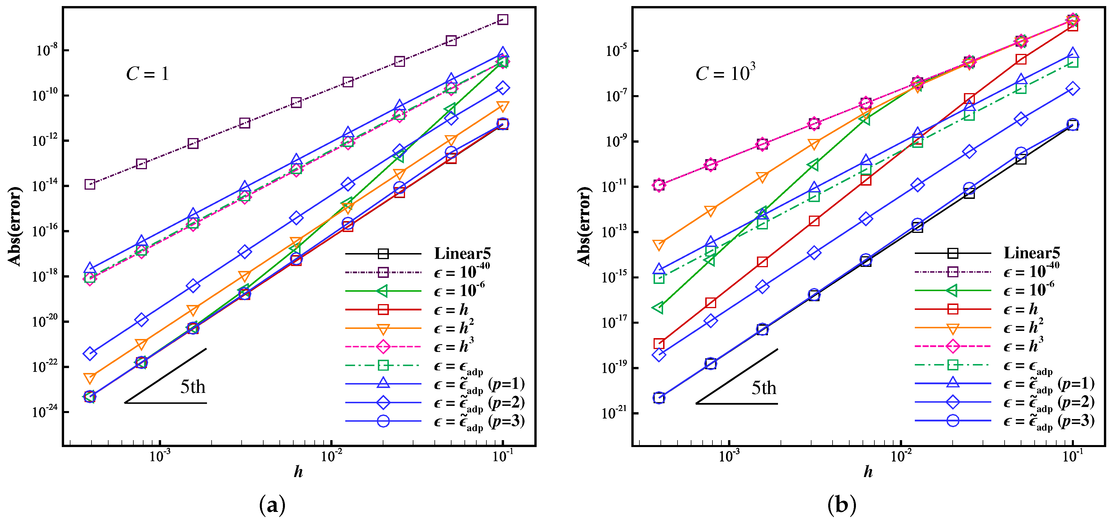
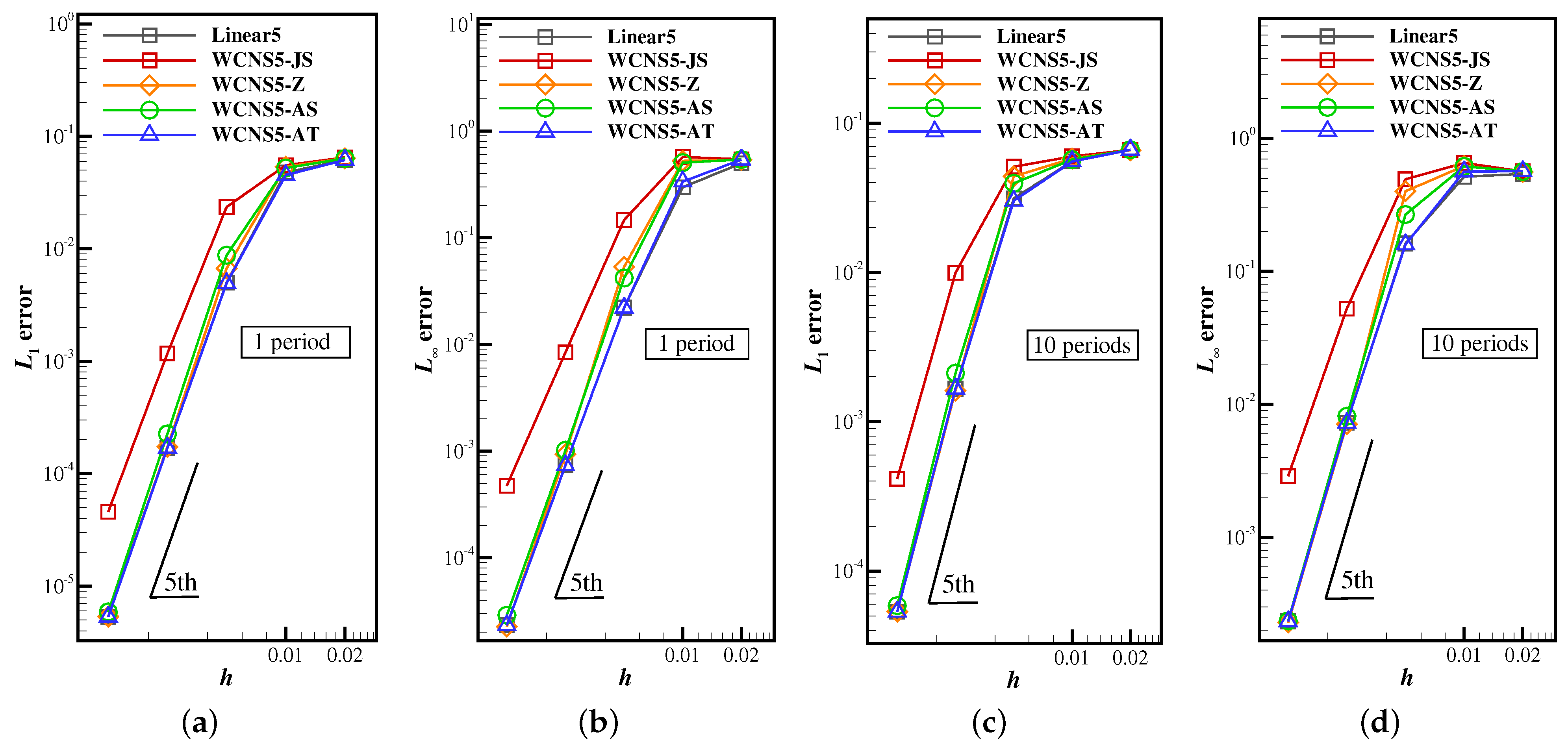
2.4.1. Convergence Accuracy

For existing convergence analysis [3,4,5], $ϵ$ was usually assumed to be 0. This subsection discusses whether the introduction of ${\widetilde{ϵ}}_{\mathrm{adp}}$ has any effect on the convergence of the WCNS5-AT scheme, i.e., whether it can achieve fifth-order accuracy in the smooth region of the flow field. Convergence at critical points will be studied in the next subsection.

First, the Taylor series expansion of smoothness indicators of each sub-stencil in Equation (14) yields

$$\begin{array}{cc}\hfill & {\beta }_0={u_j^{\prime }}^2{h}^2+\left({u_j^{″}}^2-\frac{2u_j^{\prime }{u}_j^{\left(3\right)}}{3}\right)h^4+\left(-2u_j^{″}{u}_j^{\left(3\right)}+\frac{u_j^{\prime }{u}_j^{\left(4\right)}}{2}\right)h^5+O\left(h^6\right)\hfill \\ \hfill & {\beta }_1={u_j^{\prime }}^2{h}^2+\left({u_j^{″}}^2+\frac{u_j^{\prime }{u}_j^{\left(3\right)}}{3}\right)h^4+O\left(h^6\right)\hfill \\ \hfill & {\beta }_2={u_j^{\prime }}^2{h}^2+\left({u_j^{″}}^2-\frac{2u_j^{\prime }{u}_j^{\left(3\right)}}{3}\right)h^4+\left(2u_j^{″}{u}_j^{\left(3\right)}-\frac{u_j^{\prime }{u}_j^{\left(4\right)}}{2}\right)h^5+O\left(h^6\right)\hfill \end{array}$$

(23)

If $n_{cp}=0$, it can be easily derived from Equation (23) that

$$\begin{array}{c}\hfill {\beta }_k=D(1+O\left(h^2\right))\end{array}$$

(24)

where D is a non-zero constant independent of k. From Equation (23) we know that $D=u_j^{\prime 2}{h}^2$. Expanding Equation (17) in Taylor series, we have

$$\begin{array}{c}\hfill \tau =\left|{\beta }_0-{\beta }_2\right|=\left(-4u_j^{″}{u}_j^{\left(3\right)}+u_j^{\prime }{u}_j^{\left(4\right)}\right)h^5+O\left(h^7\right)=O\left(h^5\right)\end{array}$$

(25)

From Equation (18), it can be easily deduced that

$$\begin{array}{c}\hfill \tilde{\tau }=\frac{\tau }{{\beta }_{max}}=\frac{O\left(h^5\right)}{D(1+O\left(h^2\right))}=O\left(h^3\right)\end{array}$$

(26)

Thus, using Equations (22), (24) and (26), we obtain

$$\begin{array}{cc}\hfill {\alpha }_k^{\mathrm{AT}}& =\frac{d_k{\tilde{\tau }}^{2p}}{{\left({\beta }_k{\tilde{\tau }}^p+\sigma \right)}^2}=\frac{d_k{\left(O\left(h^3\right)\right)}^{2p}}{{\left(D\left(1+O\left(h^2\right)\right){\left(O\left(h^3\right)\right)}^p+D\left(1+O\left(h^2\right)\right)\right)}^2}\hfill \\ \hfill & =\frac{d_k}{E}\left(1+O\left(h^2\right)\right)\hfill \end{array}$$

(27)

where $E=D^2/{\tilde{\tau }}^{2p}$. Considering that the linear weight $d_k$ satisfies ${\sum }_{k=0}^2{d}_k=1$, the sum of these terms ${\alpha }_k^{\mathrm{AT}}$ is given by

$$\begin{array}{c}\hfill {\displaystyle \sum _{k=0}^2}{\alpha }_k^{\mathrm{AT}}=\frac{1}{E}(1+O\left(h^2\right))\end{array}$$

(28)

Substituting Equations (27) and (28) into Equation (22) gives

$$\begin{array}{c}\hfill {\omega }_k^{\mathrm{AT}}=d_k+O\left(h^2\right)\end{array}$$

(29)

Therefore, for the JS weight function, the new weight function meets the convergence requirements in Refs. [5,20], which proves that the WCNS5-AT scheme can achieve fifth-order accuracy at non-critical points.

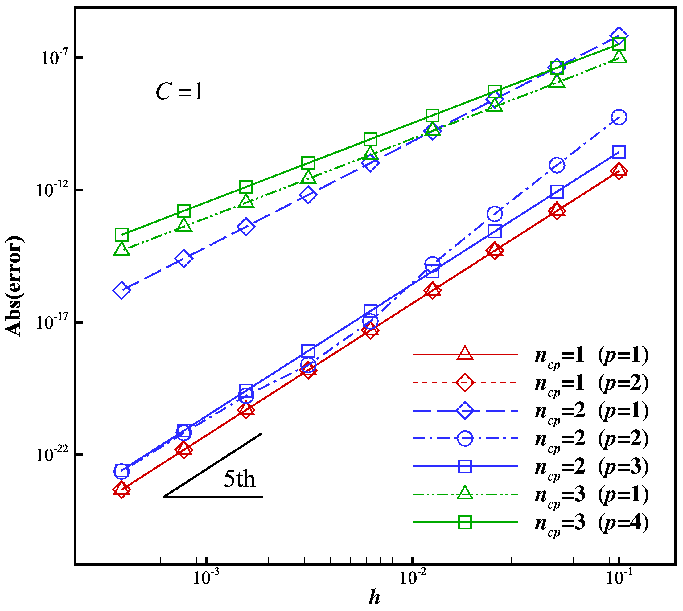
2.4.2. Convergence at Critical Points

The convergence at critical points may become more complicated. The JS weight function fails to satisfy the conditions for fifth-order convergence due to the vanishment of the low-order derivatives at critical points, which results in a loss of accuracy. In this subsection, we analytically demonstrate that the introduction of ${\widetilde{ϵ}}_{\mathrm{adp}}$ makes the JS weight function recover fifth-order convergence at critical points.

Table 1. Taylor series expansion of ${\beta }_k$ and $\tau$ for WCNS5.

${\mathit{n}}_{\mathit{c}\mathit{p}}$	${\mathit{\beta }}_0$	${\mathit{\beta }}_1$	${\mathit{\beta }}_2$	$\mathit{\tau }$
0	${u_j^{\prime }}^2{h}^2\left(1+O\left(h^2\right)\right)$	${u_j^{\prime }}^2{h}^2\left(1+O\left(h^2\right)\right)$	${u_j^{\prime }}^2{h}^2\left(1+O\left(h^2\right)\right)$	$\left(-4u_j^{″}{u}_j^{\left(3\right)}+u_j^{\prime }{u}_j^{\left(4\right)}\right)h^5\left(1+O\left(h^2\right)\right)$
1	${u_j^{″}}^2{h}^4(1+O\left(h\right))$	${u_j^{″}}^2{h}^4\left(1+O\left(h^2\right)\right)$	${u_j^{″}}^2{h}^4(1+O\left(h\right))$	$-4u_j^{″}{u}_j^{\left(3\right)}{h}^5\left(1+O\left(h^2\right)\right)$
2	$\frac{10}{9}{u}_j^{\left(3\right)2}{h}^6(1+O\left(h\right))$	$\frac{1}{36}{u}_j^{\left(3\right)2}{h}^6\left(1+O\left(h^2\right)\right)$	$\frac{10}{9}{u}_j^{\left(3\right)2}{h}^6(1+O\left(h\right))$	$-\frac{8}{3}{u}_j^{\left(3\right)}{u}_j^{\left(4\right)}{h}^7\left(1+O\left(h^2\right)\right)$
3	$\frac{29}{72}{u}_j^{\left(4\right)2}{h}^8(1+O\left(h\right))$	$\frac{1}{144}{u}_j^{\left(4\right)2}{h}^8\left(1+O\left(h^2\right)\right)$	$\frac{29}{72}{u}_j^{\left(4\right)2}{h}^8(1+O\left(h\right))$	$-\frac{7}{10}{u}_j^{\left(4\right)}{u}_j^{\left(5\right)}{h}^9\left(1+O\left(h^2\right)\right)$

gives the Taylor series expansion for ${\beta }_k$ and $\tau$ for the fifth-order WCNS scheme, which yields

$$\begin{array}{cc}\hfill {\beta }_k& =O\left(h^{2\left(n_{cp}+1\right)}\right),\hfill \\ \hfill \tau & =\left\{\begin{array}{cc}O\left(h^5\right),\hfill & n_{cp}=0\hfill \\ O\left(h^{2\left(n_{cp}+1\right)+1}\right),\hfill & n_{cp}\ge 1\hfill \end{array}\right.\hfill \\ \hfill & =O\left(h^{max\left(5,2\left(n_{cp}+1\right)+1\right)}\right)\hfill \end{array}$$

(30)

In addition, it can be seen from Table 1 that if only the first derivative vanishes, i.e., $n_{cp}=1$, then ${\beta }_{0,2}=D(1+O\left(h\right))$, implying that ${\omega }_k=d_k+O\left(h\right)$, which will cause the convergence to degrade to third-order accuracy.

For the WCNS5-AT scheme, even if ${\beta }_{0,2}=D(1+O\left(h\right))$ at first-order critical points, we still have $\sigma =min({\beta }_0,{\beta }_1,{\beta }_2)=D(1+O\left(h^2\right))$ as in Equation (28). It is not difficult to find that the fifth-order accuracy can be restored when the free parameter p satisfies a certain condition. For simplicity, this condition is determined directly based on the conclusion about $ϵ$ derived by Don and Borges [6]. Substituting Equation (30) into Equation (21), if $n_{cp}=1$, we can obtain

$$\begin{array}{c}\hfill {\widetilde{ϵ}}_{\mathrm{adp}}=\Theta \left(h^{4-p}\right)\end{array}$$

(31)

Hence, the condition ${\widetilde{ϵ}}_{\mathrm{adp}}=\mathsf{\Omega }\left(h^2\right)$ can be satisfied with $p\ge 2$, indicating that the WCNS5-AT scheme can maintain the optimal order accuracy at first-order critical points in smooth regions. Here, this theoretical conclusion will be verified by a simple numerical test.

Consider the following family of test functions [6]

$$\begin{array}{c}\hfill g_n\left(x\right)=C{e}^{0.75(x-1)}{x}^n\end{array}$$

(32)

where $x\in [-1,1]$, C is a constant, and n is a non-negative integer. $x=0$ is the only critical point with an order of $n_{cp}=n-1$. We first consider $g_2\left(x\right)=C{e}^{0.75(x-1)}{x}^2(n_{cp}=1)$. $g_2^{\prime }\left(0\right)$ is calculated using the WCNS5-JS scheme with $ϵ={10}^{-40}$, ${10}^{-6}$, h, $h^2$, $h^3$, ${ϵ}_{\mathrm{adp}}$ [18] and ${\widetilde{ϵ}}_{\mathrm{adp}}(p=1,2,3)$, respectively. Grid spacing is set as $h=0.02\times 2^n(n=1,2,...,9)$. The results of the Linear5 scheme are used as references. Figure 2 presents the error of $g_2^{\prime }\left(0\right)$ with $C=1$ and $C={10}^3$.

The results in Figure 2 indicate that when $C=1$, the small $ϵ={10}^{-40}$ yields only third-order accuracy (${\beta }_k\gg ϵ$), while the larger $ϵ={10}^{-6}$ recommended in Ref. [3] first shows super convergence, then gradually reaches the fifth-order accuracy (${\beta }_k\ll ϵ$) as grid refines. This suggests that the performance of the WCNS5-JS scheme is very sensitive to the relative magnitudes of $ϵ$ and ${\beta }_k$. More specifically, the larger value ($ϵ={10}^{-6}$) will dominate over the smoothness indicators in the refined grid, which in fact hides the deficiency of the classical JS weight function at critical points [4,5]. Setting $ϵ=\mathsf{\Omega }\left(h^2\right)$, the WCNS5-JS scheme can achieve fifth-order accuracy, whereas setting $ϵ=h^3$ or $ϵ={ϵ}_{\mathrm{adp}}$, it only has fourth-order accuracy, which is consistent with the conclusions drawn in Refs. [6,18].

Moreover, increasing the amplitude of $g_2\left(x\right)$ can also have an impact on the accuracy at the critical point. For instance, it is clear from Figure 2 that when C is increased to ${10}^3$, ${\beta }_k$ will increase synchronously. In this test, ${\beta }_k\gg ϵ={10}^{-6}$ holds in coarse grids, thus there is only third-order accuracy, leading to super convergence as grid refines. Furthermore, when $ϵ$ is set as a low power-function of grid spacing, the accuracy is also affected due to changes in the relative sizes of $ϵ$ and ${\beta }_k$, which is similar to the case using $ϵ={10}^{-6}$, such as loss of accuracy or super convergence shown in Figure 2. Therefore, the accuracy of the WCNS5-JS scheme with the aforementioned $ϵ$ may be uncertain due to the influence of the size of $ϵ$, the grid resolution and the flow variable.

It can be clearly observed from Figure 2 that the new ${\widetilde{ϵ}}_{\mathrm{adp}}(p\ge 2)$ helps the WCNS5-JS scheme achieve optimal order accuracy at first-order critical point regardless of C, which is consistent with the theoretical conclusion derived from Equation (31). In other words, ${\beta }_k\ll {\widetilde{ϵ}}_{\mathrm{adp}}$ is always satisfied near first-order critical point, and the accuracy of the WCNS5-AT scheme is not affected by grid resolution or flow variables. Moreover, when C is increased from 1 to ${10}^3$, the error increases for all schemes, while the WCNS5-AT scheme with $p\ge 2$ has the lowest error and the slowest increase of error among the nonlinear schemes. Furthermore, increasing the free parameter p in ${\widetilde{ϵ}}_{\mathrm{adp}}$ helps to further decrease the error to the level of Linear5. These results benefit from the properties of ${\widetilde{ϵ}}_{\mathrm{adp}}$ being both adaptive and scale-invariant. In conclusion, the new ${\widetilde{ϵ}}_{\mathrm{adp}}$ can help the JS weight function improve convergence accuracy and decrease nonlinear error, which provides a better choice for the scheme to maintain accuracy at critical points than other choices of $ϵ$.

For higher-order critical points $n_{cp}\ge 2$, we can also theoretically derive an expression similar to Equation (31) for ${\widetilde{ϵ}}_{\mathrm{adp}}$ to give the condition to restore the optimal order accuracy. For instance, for $n_{cp}=2$ and $n_{cp}=3$, $p\ge 4$ and $p\ge 6$ should be satisfied, respectively. Unfortunately, the situation of high-order critical points is complicated. We see in Equation (14) that ${\beta }_k$ of each sub-stencil is a combination of the first- and second-order derivatives at the stencil midpoint $x_j$. If both derivatives vanish, ${\beta }_k$ will no longer approximate non-zero quantities, and is mainly determined by the lowest order term in the Taylor series expansion [4]. As shown in Table 1, the low-order terms gradually show a difference in magnitude for $n_{cp}\ge 2$, e.g., ${\beta }_{0,2}/{\beta }_1=40$ and 58 for $n_{cp}=2$ and 3, and this difference grows rapidly as $n_{cp}$ increases. In other words, if $n_{cp}\ge 2$, then ${\beta }_k=D(1+O\left(1\right))$, implying ${\omega }_k=d_k+O\left(1\right)$, i.e., Equation (29) is not satisfied. The adaptive idea of ${\widetilde{ϵ}}_{\mathrm{adp}}$ is based on the discrepancy in ${\beta }_k$, thus ${\widetilde{ϵ}}_{\mathrm{adp}}$ is unable to solve the dilemma, which results in loss of accuracy, same as the classical WCNS scheme.

Table 2. The ${\beta }_k$, ${\omega }_k^{\mathrm{AT}}$, and ${\widetilde{ϵ}}_{\mathrm{adp}}(p=2,4,6)$ of $g_n\left(x\right)(n=2,3,4)$ near $x_j=0$ for WCNS5-AT.

${\mathit{n}}_{\mathbf{cp}}$	${\mathit{S}}_5\mathbf{Midpoint}$	${\mathit{\beta }}_0$	${\mathit{\beta }}_1$	${\mathit{\beta }}_2$	${\mathit{\omega }}_0^{\mathbf{AT}}$	${\mathit{\omega }}_1^{\mathbf{AT}}$	${\mathit{\omega }}_2^{\mathbf{AT}}$	${\widetilde{\mathit{ϵ}}}_{\mathbf{adp}}$
1	$x_{j-1}$	$2.72\times {10}^{-7}$	$2.72\times {10}^{-7}$	$2.72\times {10}^{-7}$	$6.25\times {10}^{-2}$	$6.25\times {10}^{-1}$	$3.13\times {10}^{-1}$	$3.45\times {10}^{-2}$
	$x_j$	$1.36\times {10}^{-7}$	$1.36\times {10}^{-7}$	$1.37\times {10}^{-7}$	$6.25\times {10}^{-2}$	$6.25\times {10}^{-1}$	$3.13\times {10}^{-1}$	$4.32\times {10}^{-3}$
	$x_{j+1}$	$2.72\times {10}^{-7}$	$2.73\times {10}^{-7}$	$2.73\times {10}^{-7}$	$6.25\times {10}^{-2}$	$6.25\times {10}^{-1}$	$3.13\times {10}^{-1}$	$3.45\times {10}^{-2}$
2	$x_{j-1}$	$1.92\times {10}^{-12}$	$6.90\times {10}^{-13}$	$1.33\times {10}^{-14}$	$3.86\times {10}^{-5}$	$2.92\times {10}^{-3}$	$9.97\times {10}^{-1}$	$1.36\times {10}^{-14}$
	$x_j$	$5.31\times {10}^{-13}$	$1.33\times {10}^{-14}$	$5.33\times {10}^{-13}$	$6.25\times {10}^{-2}$	$6.25\times {10}^{-1}$	$3.13\times {10}^{-1}$	$3.27\times {10}^{-5}$
	$x_{j+1}$	$1.33\times {10}^{-14}$	$6.93\times {10}^{-13}$	$1.94\times {10}^{-12}$	$9.85\times {10}^{-1}$	$1.44\times {10}^{-2}$	$9.46\times {10}^{-4}$	$1.37\times {10}^{-14}$
3	$x_{j-1}$	$1.35\times {10}^{-17}$	$1.35\times {10}^{-18}$	$4.16\times {10}^{-20}$	$7.66\times {10}^{-6}$	$7.23\times {10}^{-3}$	$9.93\times {10}^{-1}$	$4.23\times {10}^{-20}$
	$x_j$	$1.20\times {10}^{-18}$	$2.08\times {10}^{-20}$	$1.21\times {10}^{-18}$	$6.25\times {10}^{-2}$	$6.25\times {10}^{-1}$	$3.13\times {10}^{-1}$	$4.61\times {10}^{-6}$
	$x_{j+1}$	$4.16\times {10}^{-20}$	$1.35\times {10}^{-18}$	$1.36\times {10}^{-17}$	$9.65\times {10}^{-1}$	$3.49\times {10}^{-2}$	$1.84\times {10}^{-4}$	$4.23\times {10}^{-20}$

presents ${\beta }_k$, ${\omega }_k^{\mathrm{AT}}$, and ${\widetilde{ϵ}}_{\mathrm{adp}}(p=2,4,6)$ of $g_n\left(x\right)(n=2,3,4)$ with $C={10}^3$ near $x_j=0$ for the WCNS5-AT scheme, and the grid spacing is $h=6.25\times {10}^{-4}$. It can be seen from Table 2 that the difference of ${\beta }_k$ is small and ${\widetilde{ϵ}}_{\mathrm{adp}}\gg {\beta }_k$ holds for $n_{cp}=1$, indicating the dominating role of ${\widetilde{ϵ}}_{\mathrm{adp}}$ in the denominator of the JS weight function, which facilitates the recovery of linear weights with $O\left(h^2\right)$ error. Near the high-order critical points, although the absolute magnitude of ${\beta }_k$ is very small, the relative difference of ${\beta }_k$ can become very large. At these points, choosing either a relatively large constant or low power-function of grid spacing for $ϵ$ can alleviate this local disparity in smooth regions. However, ${\beta }_{max}/\tau$ approximates 1 around high-order critical points, implying ${\widetilde{ϵ}}_{\mathrm{adp}}\approx {\beta }_{min}$, then the nonlinear weights ${\omega }_k^{\mathrm{AT}}$ are $O\left(1\right)$ away from linear weights $d_k$, which means that ${\widetilde{ϵ}}_{\mathrm{adp}}$ treats high-order critical points as discontinuities. This results in an inevitable loss of accuracy. Notice that ${\widetilde{ϵ}}_{\mathrm{adp}}\gg {\beta }_k$ holds only if the stencils $S_5$ are centered at the high-order critical points $x_j$. This is mainly owing to the fact that the introduction of $\tau$ into ${\widetilde{ϵ}}_{\mathrm{adp}}$ can satisfy Equation (29), which is verified through the theoretical derivation on stencils symmetrical about critical points.

Based on previous discussion, the excessive relative disparity in ${\beta }_k$ near high-order critical points results in high gradient for both high-order critical points and discontinuities. Nonetheless, high-order critical points differ from discontinuities in essence. The flow field containing critical points with arbitrary high order is still smooth. Therefore, we can construct a new higher-order global smoothness indicator composed of local flow variables, which takes the following form

$$\begin{array}{c}\hfill \widehat{\tau }={\left(u_{j-2}-4u_{j-1}+6u_j-4u_{j+1}+u_{j+2}\right)}^2\end{array}$$

(33)

The Taylor series expansion of Equation (33) gives

$$\begin{array}{c}\hfill \widehat{\tau }=u_j^{\left(4\right)2}{h}^8+\frac{1}{3}{u}_j^{\left(4\right)}{u}_j^{\left(6\right)}{h}^{10}+O\left(h^{12}\right)\end{array}$$

(34)

indicating that $\widehat{\tau }$ is $O\left(h^8\right)$. Substituting $\tau$ by $\widehat{\tau }$ in Equation (18), we obtain a new $ϵ$, denoted by ${\widehat{ϵ}}_{\mathrm{adp}}$ hereafter, which can cover up the disparity in ${\beta }_k$ for second-order critical points. With ${\widehat{ϵ}}_{\mathrm{adp}}$, $p\ge 1$ and $p\ge 2$ need to be satisfied to achieve design order for $n_{cp}=1$ and 2, respectively, which can be derived similarly to Equation (31). Figure 3 presents the error of $g_n^{\prime }\left(0\right)$ using ${\widehat{ϵ}}_{\mathrm{adp}}$, which validates this conclusion. For $n_{cp}=3$, loss of accuracy arises due to $\theta \left(\widehat{\tau }\right)=\theta \left({\beta }_k\right)=8$. To solve this problem, a higher-order global smoothness indicator can be introduced on expanded stencils, e.g., $S_6=\left\{x_{j-2},x_{j-1},x_j,x_{j+1},x_{j+2},x_{j+3}\right\}$ can give $\widehat{\tau }=O\left(h^{10}\right)$. To sum up, ${\widehat{ϵ}}_{\mathrm{adp}}$ provides a new idea for the fifth-order WCNS scheme to avoid loss of accuracy near critical points with arbitrary high order. In fact, it may not be necessary to implement the optimal order accuracy for higher-order critical points in practical computations, since the performance of the scheme will not be substantially improved. If the optimal order accuracy is forced to be maintained, serious numerical oscillations may arise near high-order critical points and discontinuities, reducing the stability of the scheme [15,18]. Therefore, ${\widetilde{ϵ}}_{\mathrm{adp}}$ in Equation (21) is recommended. The adaptive mechanism eliminates influence of the discrepancy in ${\beta }_k$ at low-order critical points to recover optimal order accuracy, and treats high-order critical points as discontinuities to effectively suppress numerical oscillations. This will be further verified by numerical tests in Section 3.

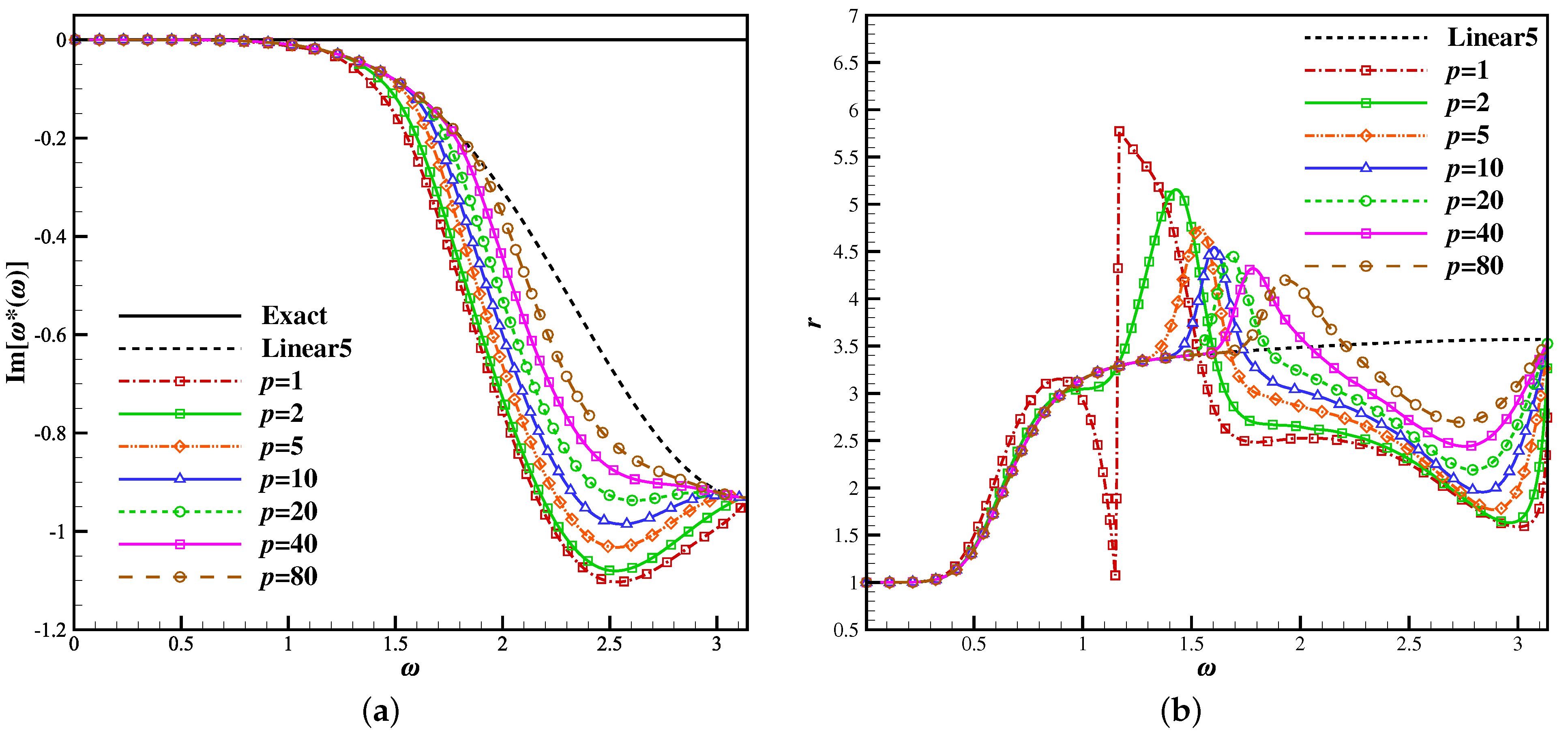
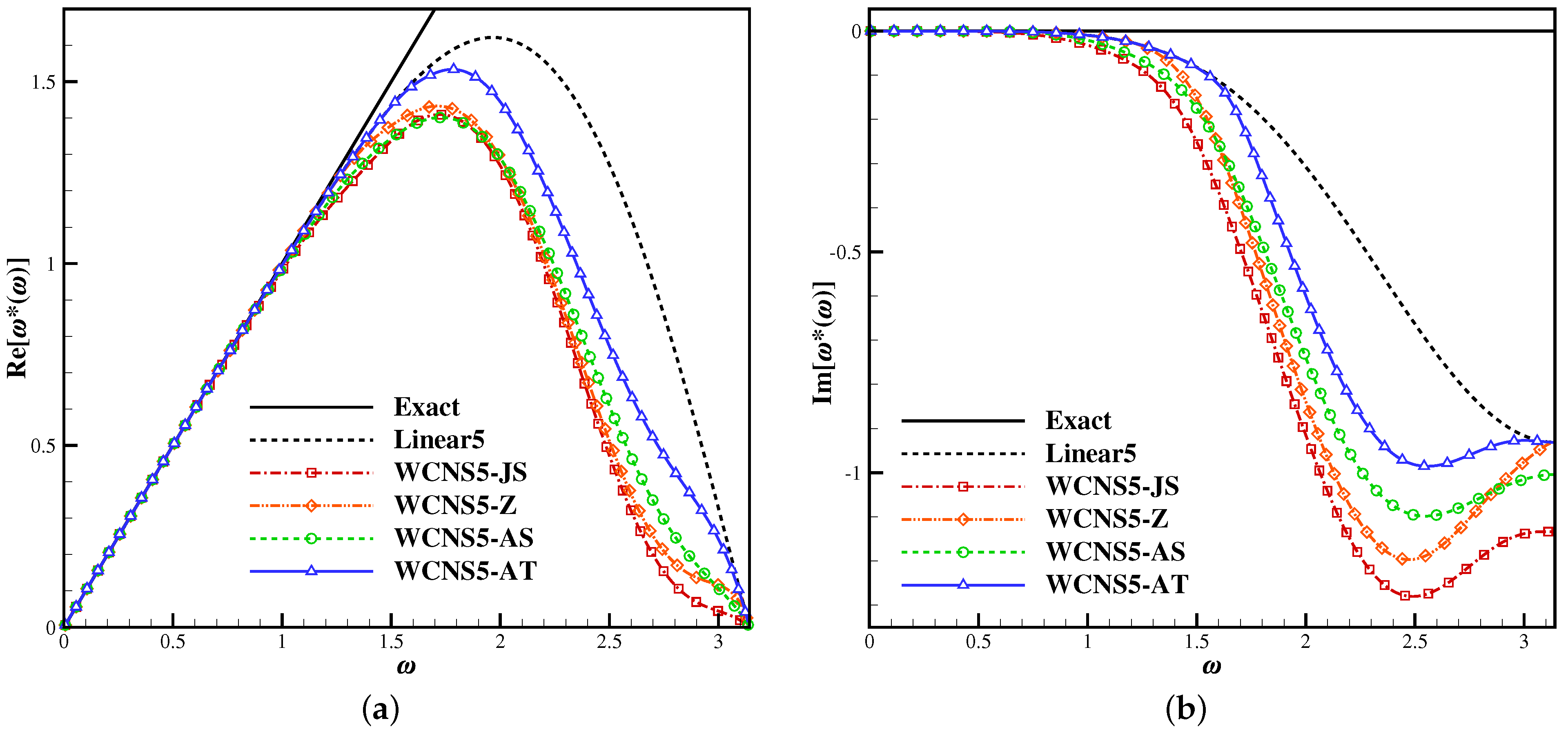
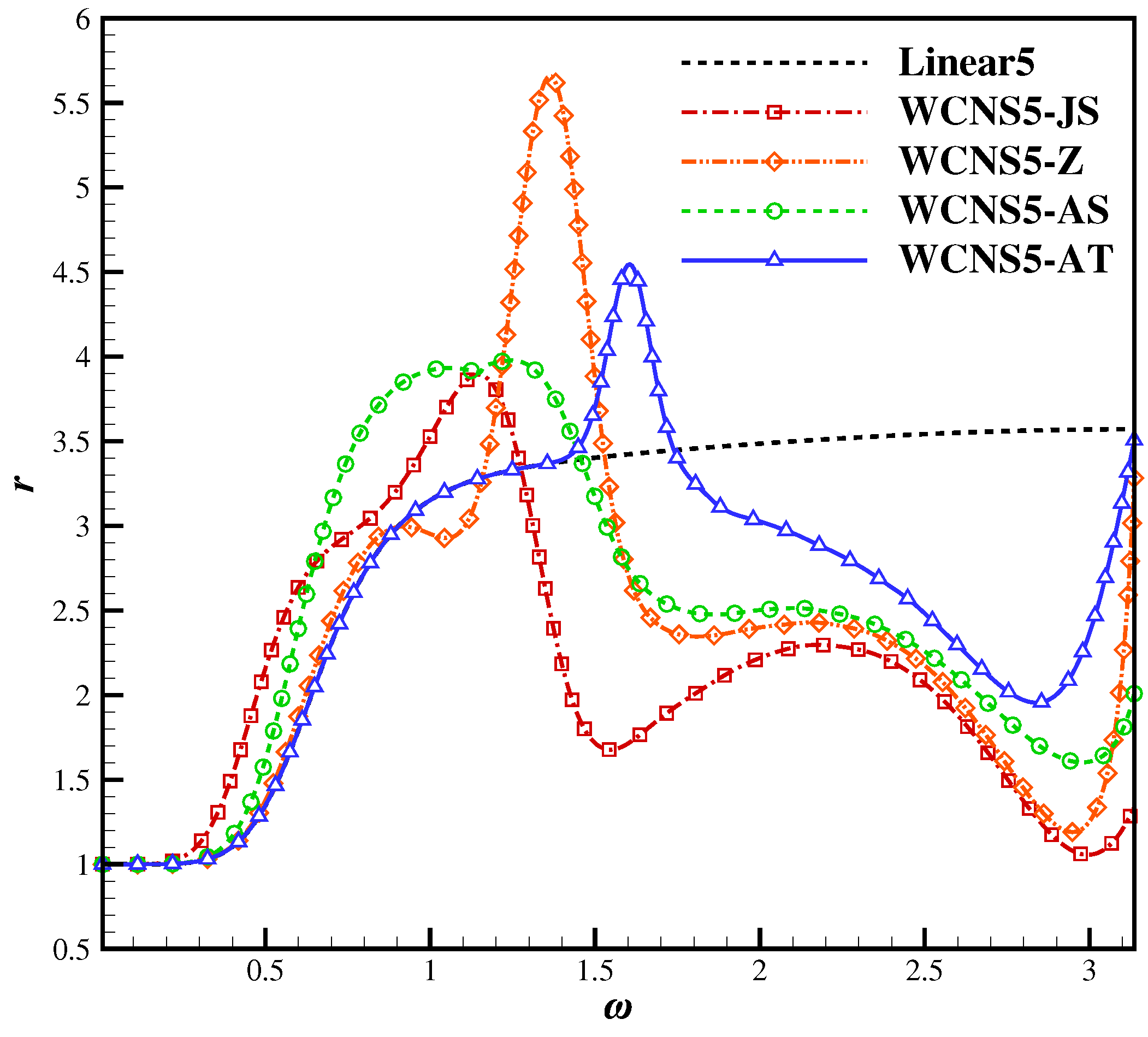
2.4.3. Spectral Properties

This subsection investigates the spectral properties of the new WCNS5-AT scheme, which is also used to determine the value of the free parameter p. Specifically, the approximate dispersion relation (ADR) [28] is used to analyze the dispersion and dissipation errors, and the minimum numerical dissipation required to damp spurious high wavenumber errors in the solution is estimated by the dispersion-dissipation relation [29]

$$\begin{array}{c}\hfill r=\frac{\left|\frac{d\left(\mathrm{Re}\left({\omega }^{*}\right)\right)}{d\omega }-1\right|+{10}^{-3}}{-\mathrm{Im}\left({\omega }^{*}\right)+{10}^{-3}}\end{array}$$

(35)

where $\mathrm{Re}\left({\omega }^{*}\right)$ and $\mathrm{Im}\left({\omega }^{*}\right)$ are the real and imaginary parts of the modified wavenumber, respectively. A smaller r indicates more numerical dissipation.

The spectral properties of the WCNS5-AT scheme with different parameter p are shown in Figure 4, where the Linear5 scheme is used as a reference to help determine the value of p. The results indicate that increasing p can improve the performance of the WCNS5-AT scheme. More specifically, the curves of the dispersion-dissipation relation with $p\ge 2$ are roughly similar. With a further increase of p, spectral properties of the WCNS5-AT scheme are highly consistent with those of the Linear5 scheme in the low wavenumber range, and the difference gradually weakens in the mid to high wavenumber range. The reason for this is that ${\widetilde{ϵ}}_{\mathrm{adp}}$ increases with p, which further conceals the disparity in smoothness indicators, thereby making the WCNS5-AT scheme approach the Linear5 scheme faster.

Nevertheless, it can also be seen from Figure 4 that the spectral error of the WCNS5-AT scheme decreases slowly for $p\ge 10$. If p is too large, the dissipation curve in the high wavenumber range will also approach the Linear5 scheme, which may intensify numerical oscillations. To balance the dispersion and dissipation errors, we hope that the WCNS5-AT scheme can still possess appropriate numerical dissipation in the high wavenumber range to suppress the non-physical oscillations, thereby ensuring the stability of the calculation. Therefore, $p=10$ with a balanced performance is used in the following sections.

Figure 5 and Figure 6 present the spectral properties of different WCNS schemes mentioned in Section 2.3. It can be clearly observed from Figure 5 that the WCNS5-JS scheme yields the largest dispersion and dissipation errors, while the new WCNS5-AT scheme has the fewest errors over the whole wavenumber range. The approximate dispersion-dissipation relation in Figure 6 shows that $0<r<5.8$ holds, which indicates that these WCNS schemes are free from spurious waves [29]. Moreover, for $\omega <1.5$, the dispersion and dissipation curves of the WCNS5-AT scheme almost coincide with those of the Linear5 scheme without exceeding it, indicating that the Linear5 scheme sets the limit of the improvement with ${\widetilde{ϵ}}_{\mathrm{adp}}$. To sum up, the introduction of the new $ϵ$ -adaptive algorithm optimizes the spectral properties of the WCNS5-JS scheme.

3. Numerical Tests

In this section, several canonical numerical tests are carried out to investigate the performance of the new WCNS5-AT scheme. These tests cover one-dimensional linear advection equation, one-dimensional Euler equations, two-dimensional Euler equations, and three-dimensional Navier–Stokes equations. It is verified that the WCNS5-AT scheme has high-resolution, good discontinuity capturing ability, and high computational efficiency compared with the classical WCNS5-JS, WCNS5-Z, and WCNS5-AS schemes. For the Euler and Navier–Stokes equations, the convective fluxes at cell-edges are evaluated by the Steger-Warming′s splitting method [30], and the characteristic decomposition is used in the nonlinear interpolation to suppress numerical oscillations near discontinuities. The strong stability preserving (SSP) third-order Runge–Kutta scheme [31] is chosen for time discretization.

3.1. One-Dimensional Linear Advection Equation

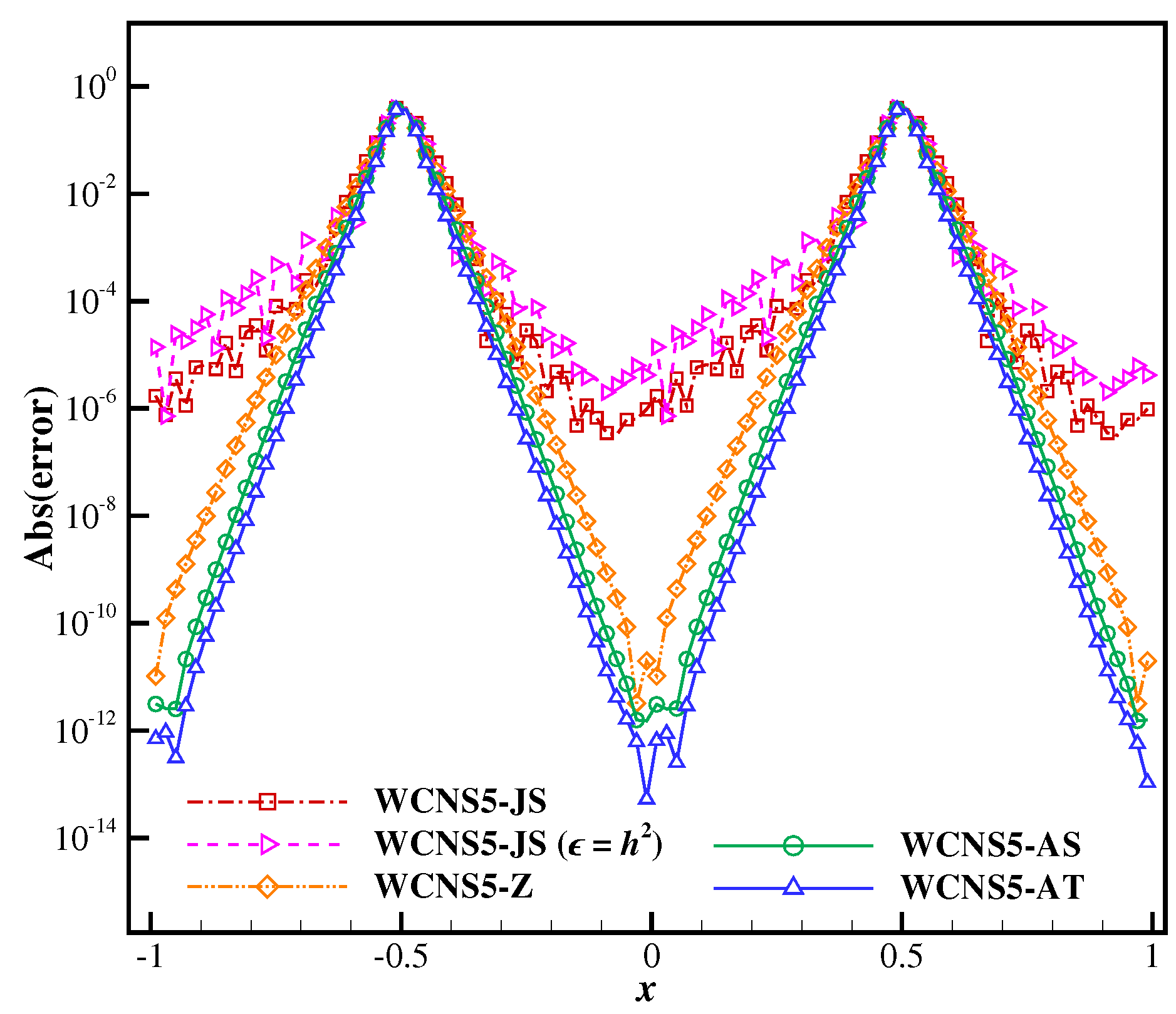
3.1.1. Wave Packet

The one-dimensional multi-scale wave packet problem is used to validate the convergence order of proposed schemes. The initial condition is $u_0\left(x\right)=\frac{1}{20}{\sum }_{k=1}^{20}sin\left(2\pi kx\right),x\in [0,1]$, with $1+25\times 2^n(n=1,2,3,4,5)$ grid points. The time step $dt$ is bounded by $0.5h^{5/3}$ to eliminate the influence of time discretization error on the convergence accuracy. For one-dimensional linear advection tests, periodic boundary conditions are applied to the left and right boundaries if not specified.

Figure 7 presents $L_1$ and $L_{\infty }$ errors of different WCNS schemes after advancing by 1 and 10 advection periods. It is evident that all schemes achieve fifth-order accuracy as grid refines. The WCNS5-JS scheme has larger errors than others, while the introduction of ${\widetilde{ϵ}}_{\mathrm{adp}}$ reduces the error level to that of the Linear5 scheme. This shows that ${\widetilde{ϵ}}_{\mathrm{adp}}$ can effectively reduce the nonlinear error and help the nonlinear scheme approach the corresponding linear scheme in smooth regions, which is more remarkable for 10 advection periods.

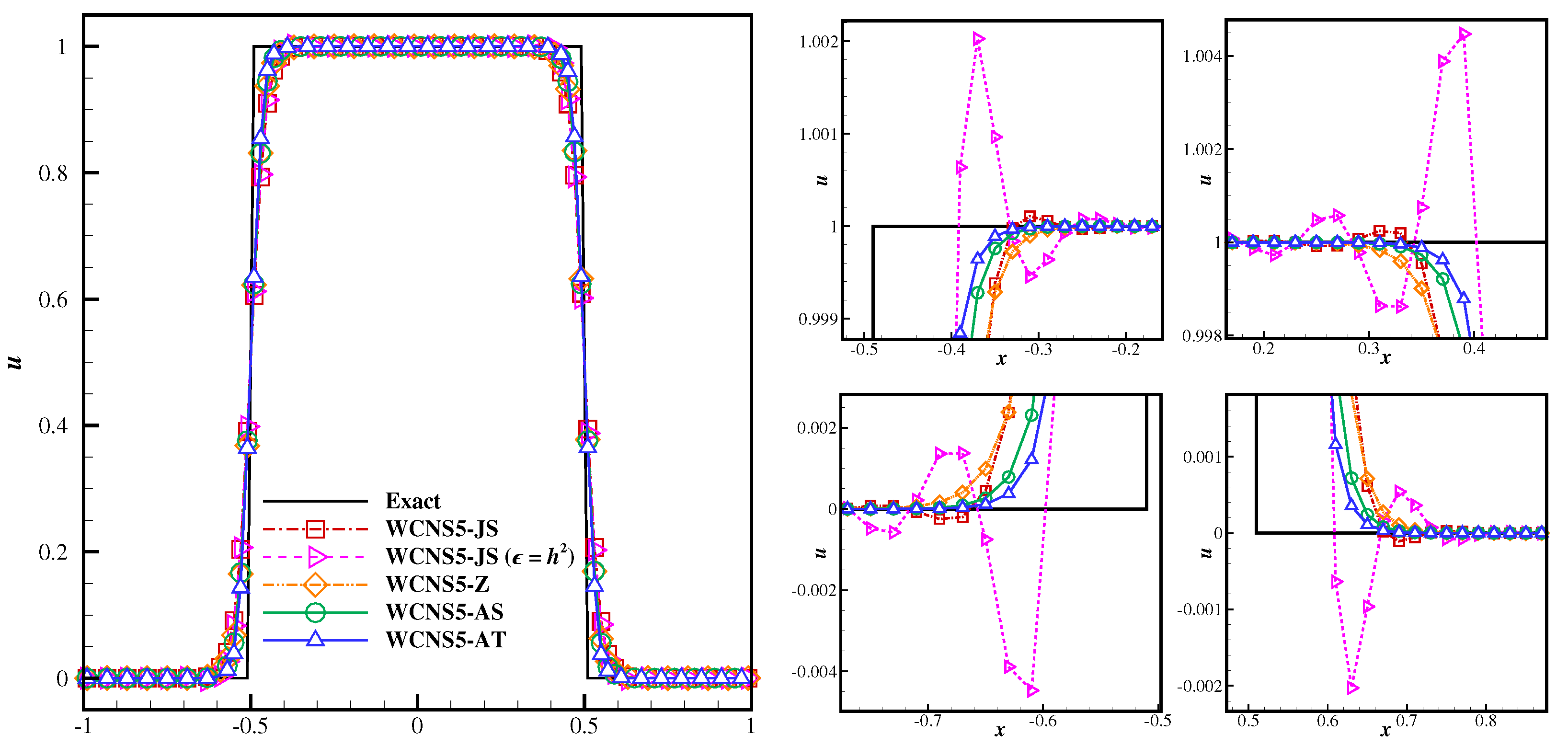
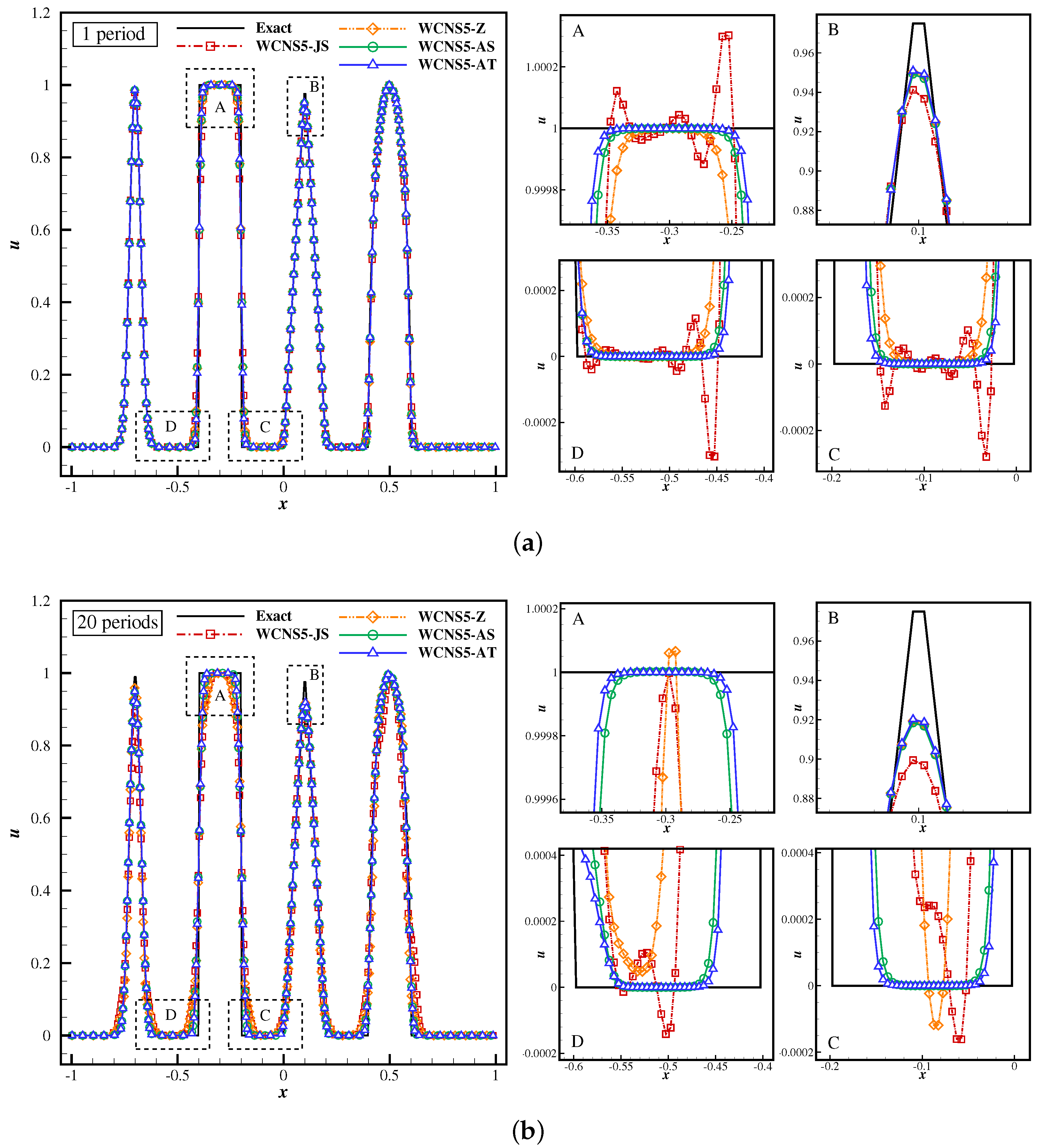
3.1.2. Square Wave

The ability to capture discontinuity is tested on a square wave. The computation is advanced to 1 advection period, with 101 grid points and CFL = 0.1.

Figure 8 and Figure 9 present the computational results and error distribution, respectively. It can be observed that the WCNS5-AT scheme significantly outperforms the WCNS5-JS, WCNS5-Z, and WCNS5-AS schemes. The WCNS5-AT scheme yields the highest resolution for discontinuities and the lowest error across the computational domain. Moreover, the previously discussed WCNS5-JS scheme with $ϵ=h^2$ is also tested, and the results are shown in Figure 8 and Figure 9, which indicate that serious numerical oscillations and large errors arise in discontinuous regions and smooth regions, respectively. Therefore, choosing $ϵ=h^2$ will damage the quality of the flow field and the convergence of numerical calculations, which is consistent with conclusions in Ref. [15] and Section 2.3.1. ${\widetilde{ϵ}}_{\mathrm{adp}}$ helps improve resolution without numerical oscillations near discontinuities.

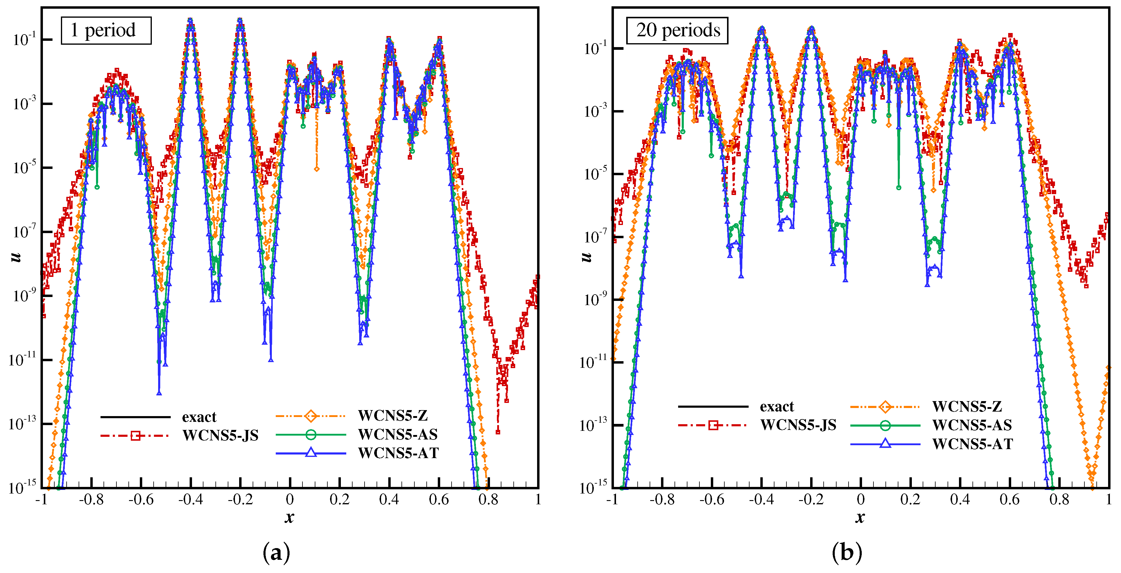
3.1.3. Composite Wave

The composite wave [3] formed by a Gaussian wave, a square wave, a triangle wave, and a semi-elliptical wave is adopted to investigate the ability to resolve various waveforms. The initial condition is as follows

$$\begin{array}{c}\hfill u(x,0)=\left\{\begin{array}{cc}\left[G\right(x,\beta ,z-\delta )+4G(x,\beta ,z)+G(x,\beta ,z+\delta \left)\right]/6\hfill & x\in [-0.8,-0.6]\hfill \\ 1\hfill & x\in [-0.4,-0.2]\hfill \\ 1-\left|10\right(x-0.1\left)\right|\hfill & x\in [0,0.2]\hfill \\ \left[F\right(x,\alpha ,a-\delta )+4F(x,\alpha ,a)+F(x,\alpha ,a+\delta \left)\right]/6\hfill & x\in [0.4,0.6]\hfill \\ 0\hfill & \mathrm{else}\hfill \end{array}\right.\end{array}$$

(36)

where $G(x,\beta ,z)={\mathrm{e}}^{-\beta {(x-z)}^2}$, $F(x,\alpha ,a)=\sqrt{max(1-{\alpha }^2{(x-a)}^2,0)}$, $\beta =log2/36{\delta }^2$, $\delta =0.005$, $z=-0.7$, $a=0.5$, $\alpha =10$. The computation is advanced to 1 and 20 advection periods, with 401 grid points and CFL = 0.1.

Computational results and error distribution are given in Figure 10 and Figure 11, respectively. It can be seen that ${\widetilde{ϵ}}_{\mathrm{adp}}$ can help the WCNS5-JS scheme to improve the resolution of various waveforms, which is basically consistent with the conclusion obtained from the square wave test. An important indicator for evaluating the shock-capturing scheme is the suppression effect on numerical oscillations near discontinuities. The JS weight function with a constant $ϵ$ induces relatively large numerical oscillations near discontinuous and large gradient smooth regions, and contaminates the numerical solutions in the upstream and downstream, which poses a great risk to the stability of the calculation. With ${\widetilde{ϵ}}_{\mathrm{adp}}$, these numerical oscillations are significantly suppressed and the error in smooth regions is maintained at a very low level. Notice that although the magnitude of the numerical oscillations in WCNS5-JS is visually small, for problems, such as aeroacoustics and turbulence, which are sensitive to small disturbances, these numerical oscillations should be handled carefully in the calculations.

For 20 advection periods, the waveforms computed using WCNS5-JS and WCNS5-Z are distorted, and large errors arise due to excessive dissipation, while the WCNS5-AT scheme maintains the waveform with the least distortion. This indicates that the WCNS5-AT scheme has the lowest numerical dissipation, which is desirable for long-time simulations.

3.2. One-Dimensional Euler Equations

3.2.1. Shock Tube Problem

This example is a canonical example to evaluate the shock-capturing ability. We consider the typical shock tube problems of Lax [32] and Sod [33], and the initial condition is given by

$$\begin{array}{cc}\hfill \mathrm{Lax}:(\rho ,u,p)& =\left\{\begin{array}{cc}(0.445\lambda ,0.698,3.528\lambda ),\hfill & x\in [0,5]\hfill \\ (0.5\lambda ,0,0.571\lambda ),\hfill & x\in (5,10]\hfill \end{array}\right.\hfill \\ \hfill \mathrm{Sod}:(\rho ,u,p)& =\left\{\begin{array}{cc}(1,0,1),\hfill & x\in [0,5]\hfill \\ (0.125,0,0.1),\hfill & x\in (5,10]\hfill \end{array}\right.\hfill \end{array}$$

(37)

where the scale factor $\lambda$ is introduced to validate the scale-invariant property of the WCNS5-AT scheme. The computation is advanced to $t=1.3$ and $t=2.0$, respectively, with 201 grid points and CFL = 0.1.

Figure 12 compares the density distribution given by WCNS5 schemes with exact solutions for $\lambda =1$. The introduction of ${\widetilde{ϵ}}_{\mathrm{adp}}$ not only improves resolution for discontinuities, but also suppresses the numerical oscillations.

Figure 13 presents the result of the Lax problem with a smaller scale $\lambda ={10}^{-3}$. It can be observed that when the scale is reduced, the constant $ϵ$ conceals the difference of smoothness indicators in both smooth and discontinuous regions, which will aggravate numerical oscillations near discontinuities for the WCNS5-JS scheme, while ${\widetilde{ϵ}}_{\mathrm{adp}}$ makes the WCNS5-JS scheme scale-invariant of flow variables, yielding consistently good performance. Notice that the scale-invariance is nearly achieved for the WCNS5-Z scheme due to the much smaller $ϵ$ (${10}^{-40}$) used in Equation (13), which is valid for most practical computations. In short, the new $ϵ$-adaptive algorithm provides a good choice to make nonlinear schemes scale-invariant of flow variables.

3.2.2. Shu-Osher Problem

This example describes the interaction between a Mach 3 right-traveling shock and an entropy wave [34]. The entropy wave is compressed and amplified through the shock, and a series of sound waves propagating downstream are produced. It is widely used to investigate the resolution of the numerical schemes for shocks and high-frequency waves. The initial condition is as follows:

$$\begin{array}{c}\hfill (\rho ,u,p)=\left\{\begin{array}{cc}(3.857143,2.629369,10.333333),\hfill & x\in [-5,-4]\hfill \\ (1+0.2sin5x,0,1),\hfill & x\in (-4,5]\hfill \end{array}\right.\end{array}$$

(38)

The computation is advanced to $t=1.8$, with 201 grid points and CFL = 0.1. Figure 14 presents density distribution results. The reference solution is given by the WCNS5-JS scheme using 6401 grid points. Compared with other WCNS5 schemes, the WCNS5-AT scheme yields higher resolution for both shocks and smooth waves, especially for the high-frequency waves behind the main shock.

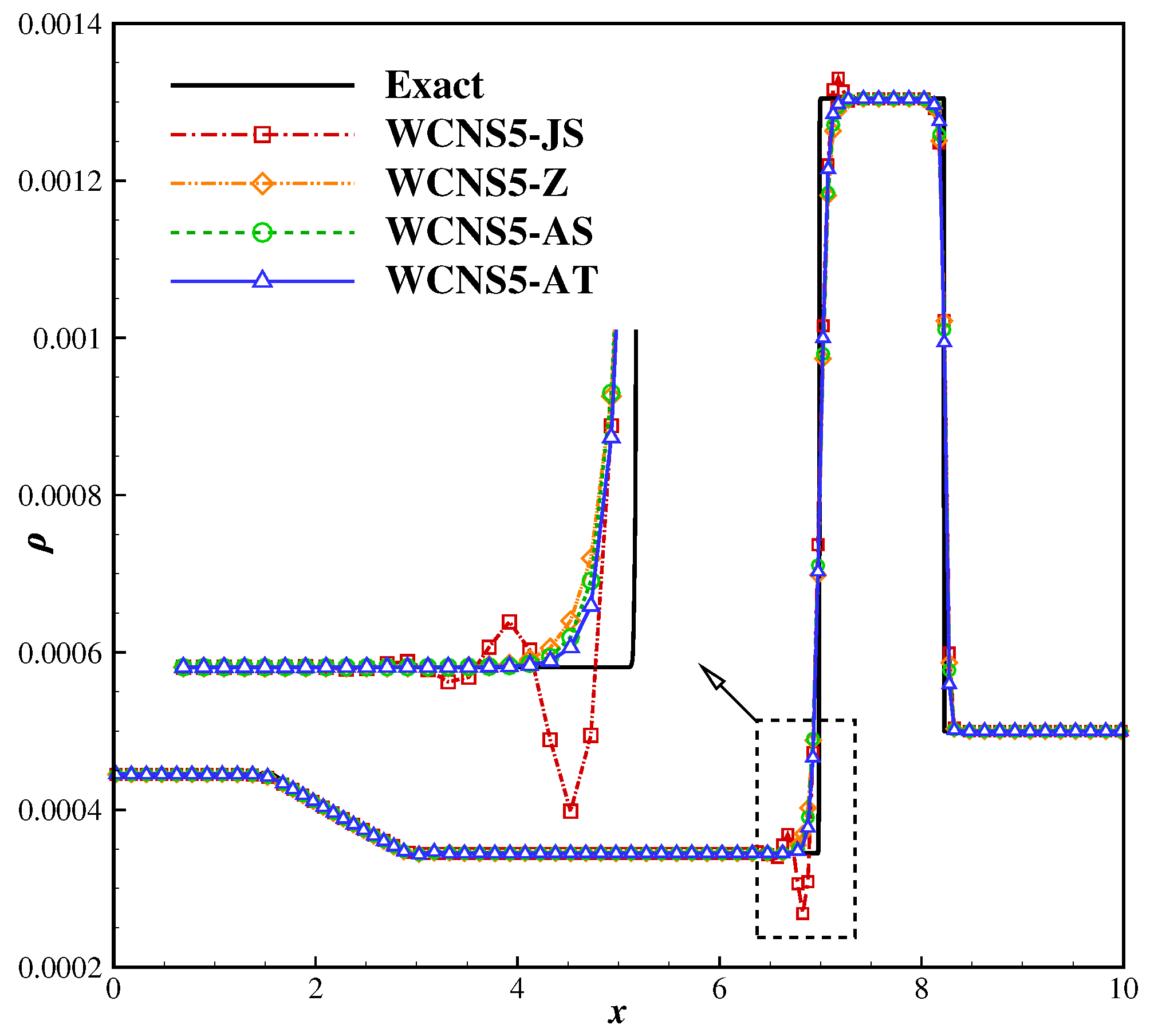
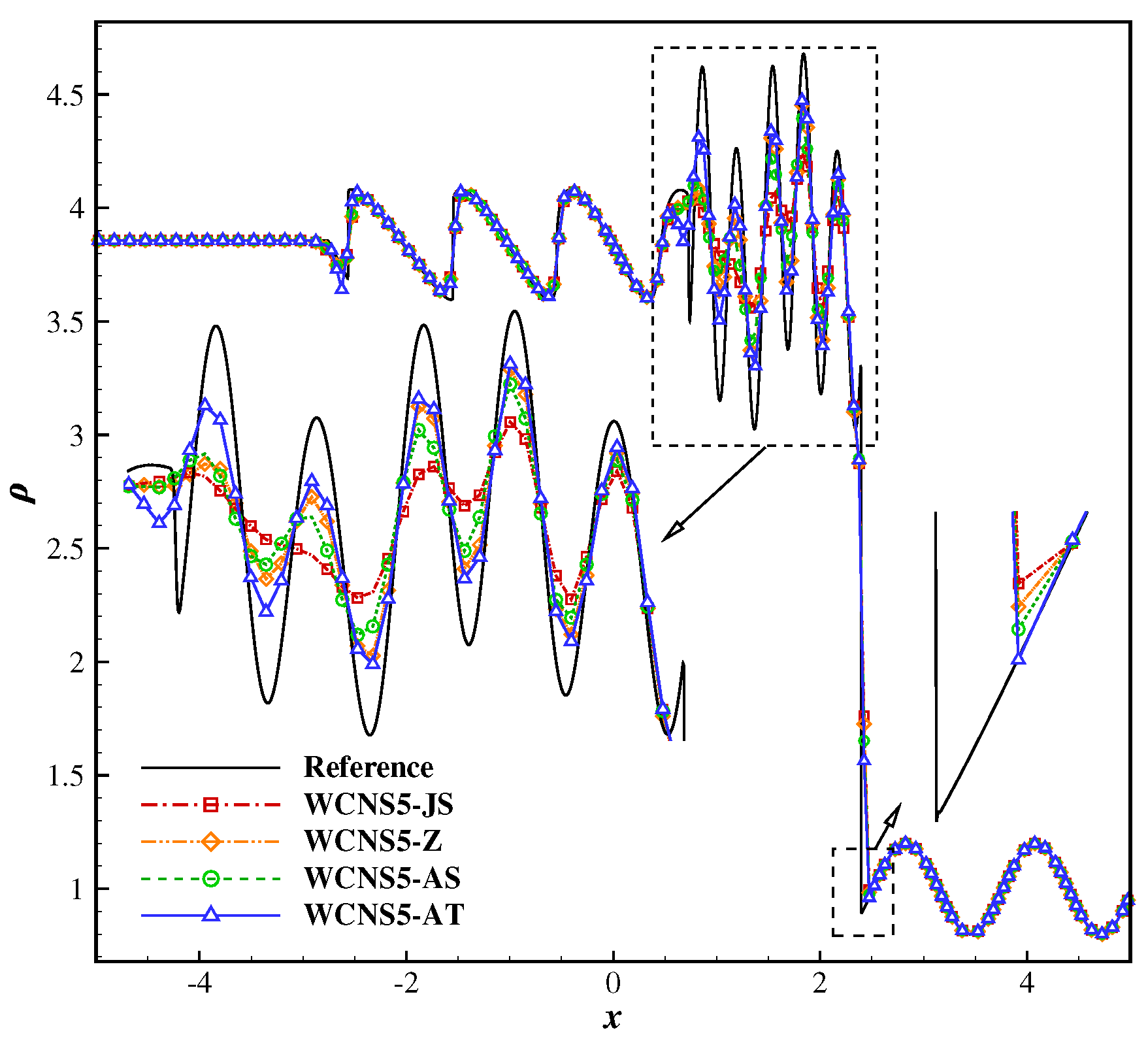
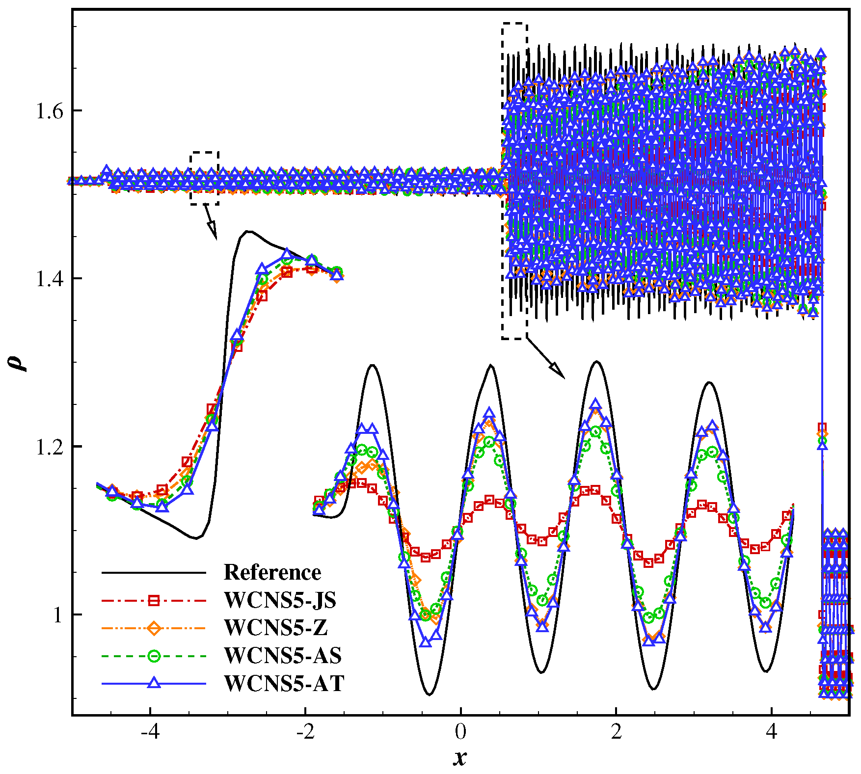
3.2.3. Titarev-Toro Problem

This example is a variant of the Shu-Osher [34] problem. The entropy wave has a higher frequency, which is a more challenging test [35]. The initial condition is

$$\begin{array}{c}\hfill (\rho ,u,p)=\left\{\begin{array}{cc}(1.515695,0.523346,1.805),\hfill & x\in [-5,-1.5]\hfill \\ (1+0.1sin20\pi x,0,1),\hfill & x\in (-1.5,5]\hfill \end{array}\right.\end{array}$$

(39)

The computation is advanced to $t=4.0$, with 1601 grid points and CFL = 0.1. The reference solution is obtained with the WCNS5-JS scheme using 6401 grid points. Results of density distribution are presented in Figure 15. The wave magnitude computed by the WCNS5-JS scheme attenuates rapidly after passing through the shock wave, while the WCNS5-Z, WCNS5-AS, and WCNS5-AT schemes can resolve high-frequency waves more accurately. The WCNS5-AT scheme has the highest resolution without spurious amplification of high-frequency waves.

3.3. Two-Dimensional Euler Equations

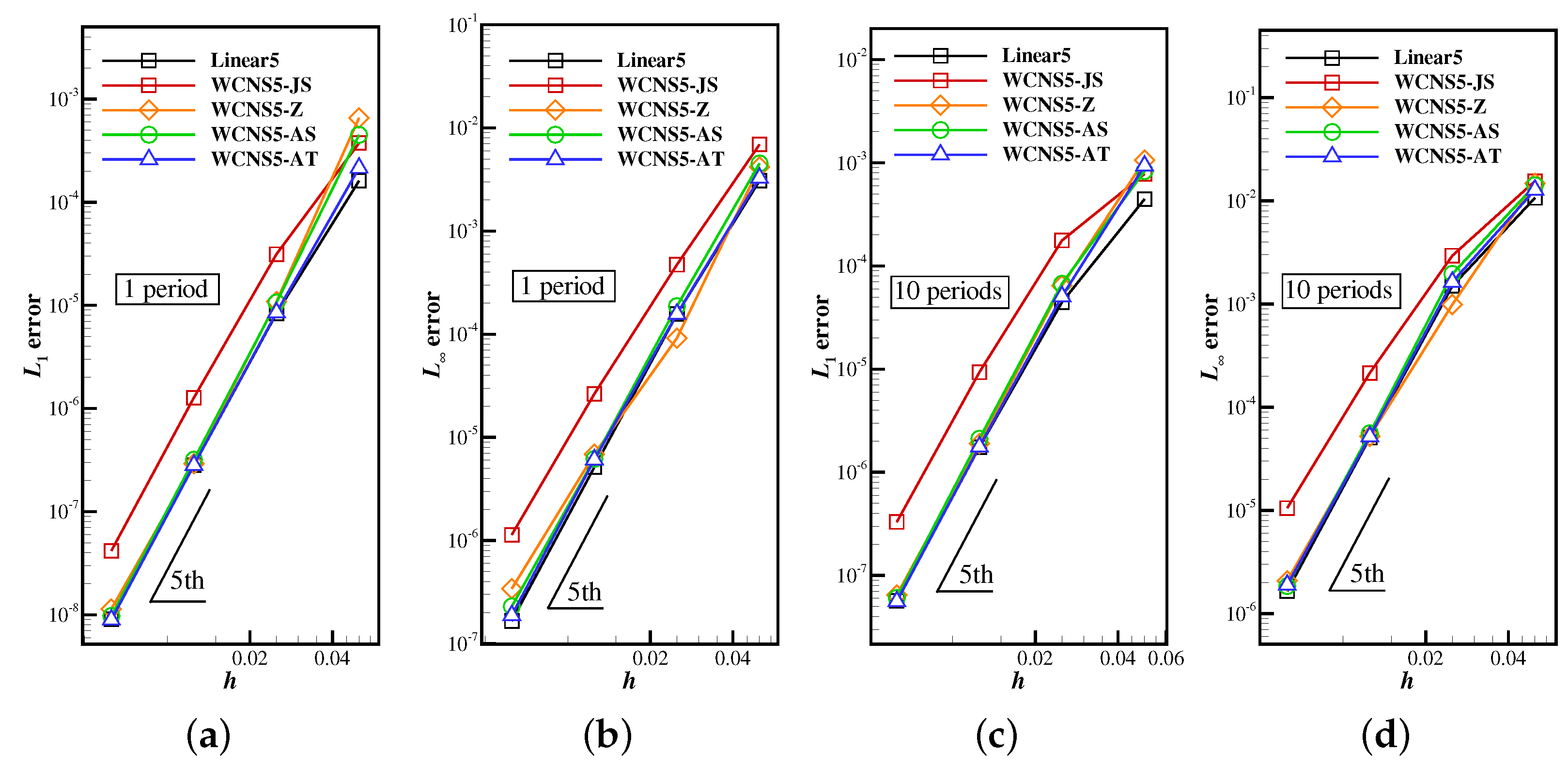
3.3.1. Isentropic Vortex Transport

The vortex transport problem [36] is used for accuracy test. This example simulates the motion of an isentropic vortex superimposed on the uniform flow of $(\rho ,u,v,p)=(1,1,0,1)$. The temperature is given by $T=p/\rho$, and the entropy is given by $S=p/{\rho }^{\gamma }$. The perturbation in velocity and temperature caused by the vortex is

$$\begin{array}{cc}\hfill (\delta u,\delta v)& =\frac{\alpha }{2\pi }exp\left(0.5\left(1-r^2\right)\right)(-\overline{y},\overline{x})\hfill \\ \hfill \delta T& =-\frac{(\gamma -1){\alpha }^2}{8\gamma {\pi }^2}exp\left(1-r^2\right)\hfill \end{array}$$

(40)

where $(x_c,y_c)=(5,5)$ is the center of the vortex, $r^2={\overline{x}}^2+{\overline{y}}^2$, and vortex strength $\alpha =1$. The computational domain is set as $[0,10]\times [0,10]$, with periodic boundary conditions in both directions. The time step is $dt=0.5h^{5/3}$ with $[1+10\times 2^n]\times [1+10\times 2^n](n=1,2,3,4)$ grid points.

Figure 16 presents $L_1$ and $L_{\infty }$ errors of density for 1 and 10 advection periods. All schemes achieve fifth-order accuracy as grid refines. The WCNS5-Z, WCNS5-AS, and WCNS5-AT schemes can greatly reduce the nonlinear error compared with the WCNS5-JS scheme, while the error level of the WCNS5-AT scheme is closest to that of the Linear5 scheme.

3.3.2. Two-Dimensional Riemann Problem

This example contains multi-scale complex structures with the interaction of shock waves, vortices, and contact discontinuities, which can test the resolution of the numerical schemes [37]. The computational domain is set as $[0,1]\times [0,1]$ with the following initial condition.

$$\begin{array}{c}\hfill (\rho ,u,v,p)=\left\{\begin{array}{cc}(1.5,0.0,0.0,1.5),\hfill & 0.8\le x\le 1,0.8\le y\le 1\hfill \\ (0.5323,1.2,0,0.3),\hfill & 0\le x<0.8,0.8\le y\le 1\hfill \\ (0.138,1.206,1.206,0.029),\hfill & 0\le x<0.8,0\le y<0.8,\hfill \\ (0.5323,0.0,1.206,0.3),\hfill & 0.8<x\le 1,0\le y<0.8\hfill \end{array}\right.\end{array}$$

(41)

The computation is advanced to $t=0.8$, with 401 × 401 grid points and CFL = 0.5. The results calculated by different fifth-order WCNS schemes are given in Figure 17. It can be seen that the WCNS5-Z and WCNS5-AS schemes yield similar resolution higher than the WCNS5-JS scheme. In contrast, the WCNS5-AT scheme captures more details of the vortex structures, indicating excellent multi-scale resolution.

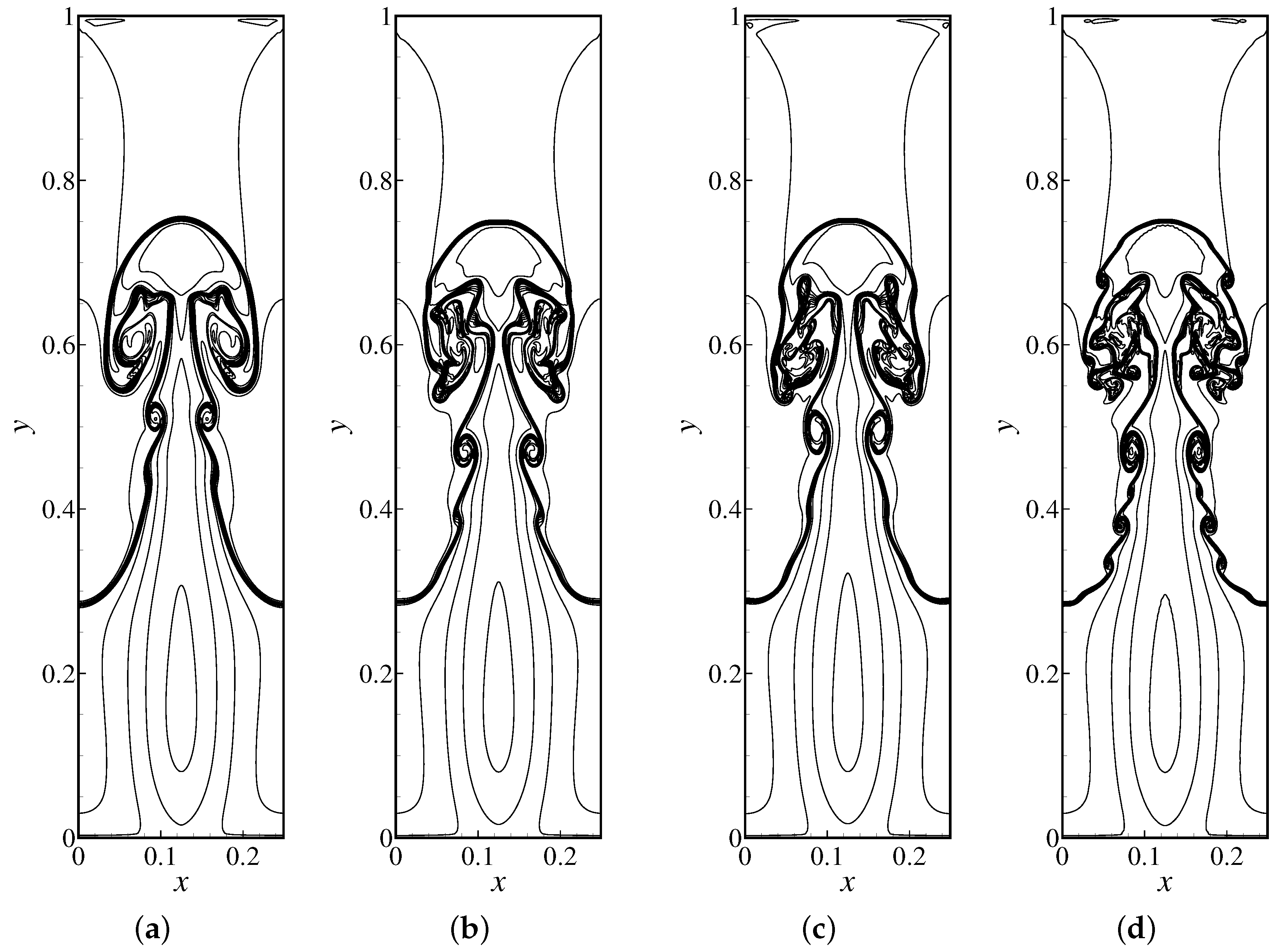
3.3.3. Rayleigh-Taylor Instability

This example describes the motion of two fluids with different densities in the initial flow field [38]. With a disturbance of the vertical velocity, the initial interface between the two fluids becomes unstable, and finally forms a complex flow field containing fine-scale structures, which can be used to examine the resolution of the numerical schemes. The computational domain is set as $[0,0.25]\times [0,1]$, and the initial condition is given by

$$\begin{array}{c}\hfill (\rho ,u,v,p)=\left\{\begin{array}{cc}(2,0,-0.025\sqrt{\gamma p/\rho }·cos\left(8\pi x\right),2y+1),\hfill & 0⩽y<0.5\hfill \\ (1,0,-0.025\sqrt{\gamma p/\rho }·cos\left(8\pi x\right),y+1.5),\hfill & 0.5⩽y<1\hfill \end{array}\right.\end{array}$$

(42)

where $\gamma =5/3$ is the specific heat ratio. A source term $S=(0,0,\rho ,\rho v)$ is added to the right-hand side of the Euler equations to simulate the gravity effect. The left and right boundaries are set with reflective conditions, and the upper and lower boundaries are imposed with fixed values

$$\begin{array}{c}\hfill (\rho ,u,v,p)=\left\{\begin{array}{cc}(1,0,0,2.5),\hfill & y=1\hfill \\ (2,0,0,1),\hfill & y=0\hfill \end{array}\right.\end{array}$$

(43)

The computation is advanced to $t=1.95$, with 241 × 961 grid points and CFL = 0.5. The results of density contours are shown in Figure 18. It is evident that the WCNS5-AT scheme yields the highest resolution of flow field. Specifically, small-scale flow structures near $y=0.35$ and 0.65 are clearly captured compared with the other three schemes. This indicates that ${\widetilde{ϵ}}_{\mathrm{adp}}$ helps reduce the numerical dissipation, and effectively improves the resolution of small-scale structures in smooth regions.

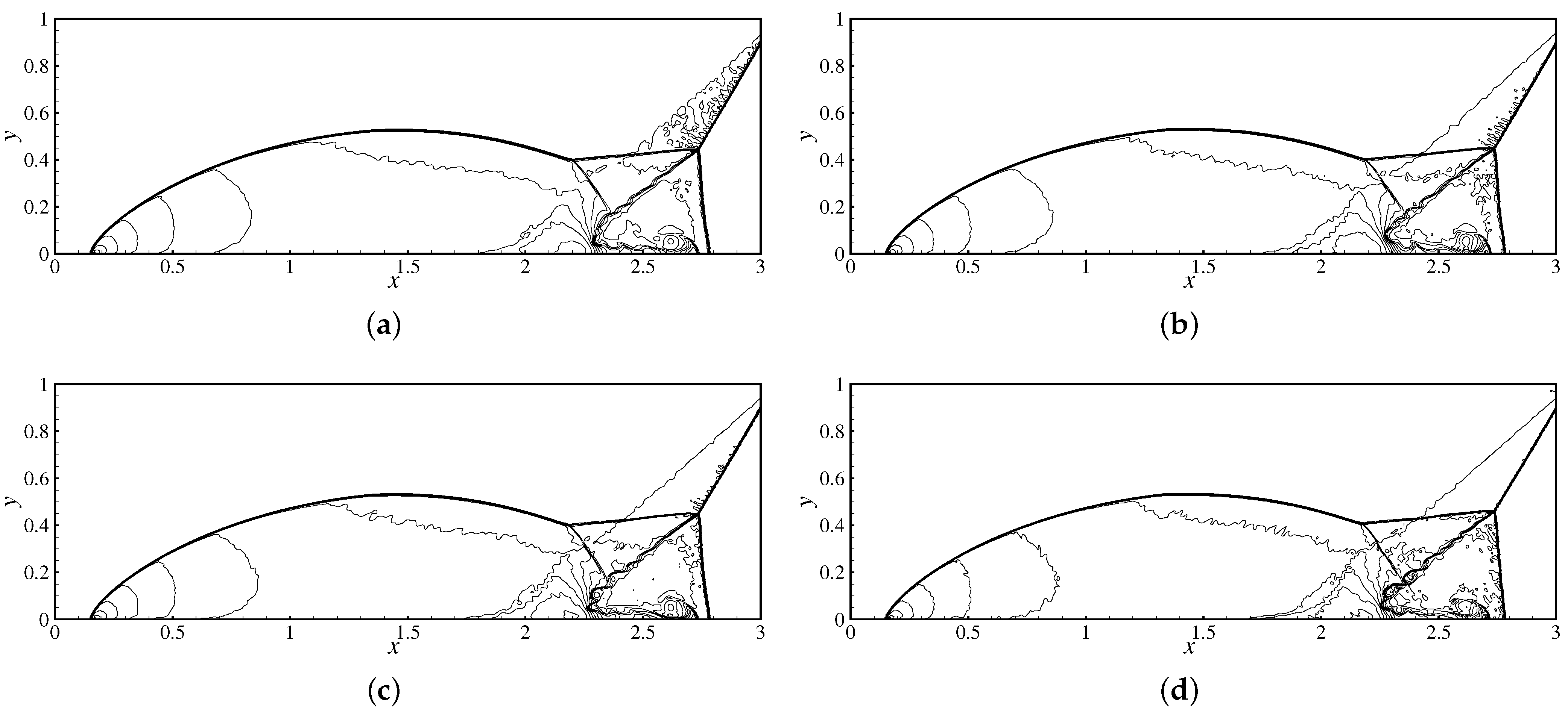
3.3.4. Double Mach Reflection

This example describes a Mach 10 shock moving from left to right along the x-axis initially with an incident angle of ${60}^{\circ }$ [39]. It is widely used to examine the resolution capability of numerical formats for strong discontinuities and small-scale structures in the resulting flow field. The computational domain is set as $[0,4]\times [0,1]$, with initial condition as follows

$$\begin{array}{c}\hfill (\rho ,u,v,p)=\left\{\begin{array}{cc}\left(8,8.25cos\frac{\pi }{6},-8.25sin\frac{\pi }{6},116.5\right),\hfill & x\le \frac{1}{6}+\frac{y}{tan\frac{\pi }{3}}\hfill \\ (1.4,0,0,1),\hfill & x>\frac{1}{6}+\frac{y}{tan\frac{\pi }{3}}\hfill \end{array}\right.\end{array}$$

(44)

where the top boundary of the computational domain describes the exact motion of the shock, the bottom boundary is imposed as the post-shock state for $x\le 1/6$ and the reflective wall for $x>1/6$, and the left and right boundary are fixed at post-shock and pre-shock state, respectively. The computation is advanced to $t=0.2$, with 961 × 241 grid points and CFL = 0.5. Figure 19 presents the result of density contours. It can be seen that the WCNS5-AT scheme yields the highest resolution for small-scale vortices rolled up along the slip line with clear capture of shocks and Mach stems.

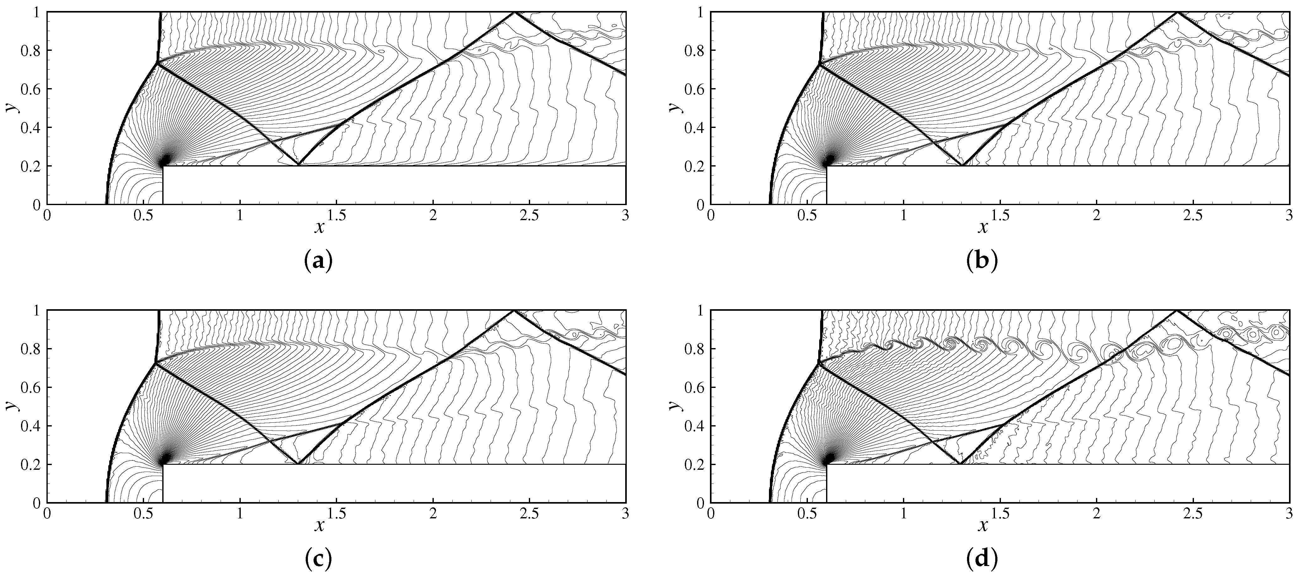
3.3.5. Forward Facing Step

This example describes a Mach 3 shock entering the wind tunnel with a front step and generating an off-body shock at the head, followed by multiple reflections on the walls [39]. This is often used to investigate the resolution and stability of numerical schemes. The reflective boundary condition is imposed for the wind tunnel and the step, and the inflow condition and outflow condition are set for the left and right boundary, respectively. The computational domain is set as $[0,4]\times [0,1]$, and the computation is advanced to $t=4.0$, with 601 × 201 grid points and CFL = 0.5. The density contours shown in Figure 20 indicate that the WCNS5-AT scheme captures the vortices rolled up along the slip line more clearly than other schemes.

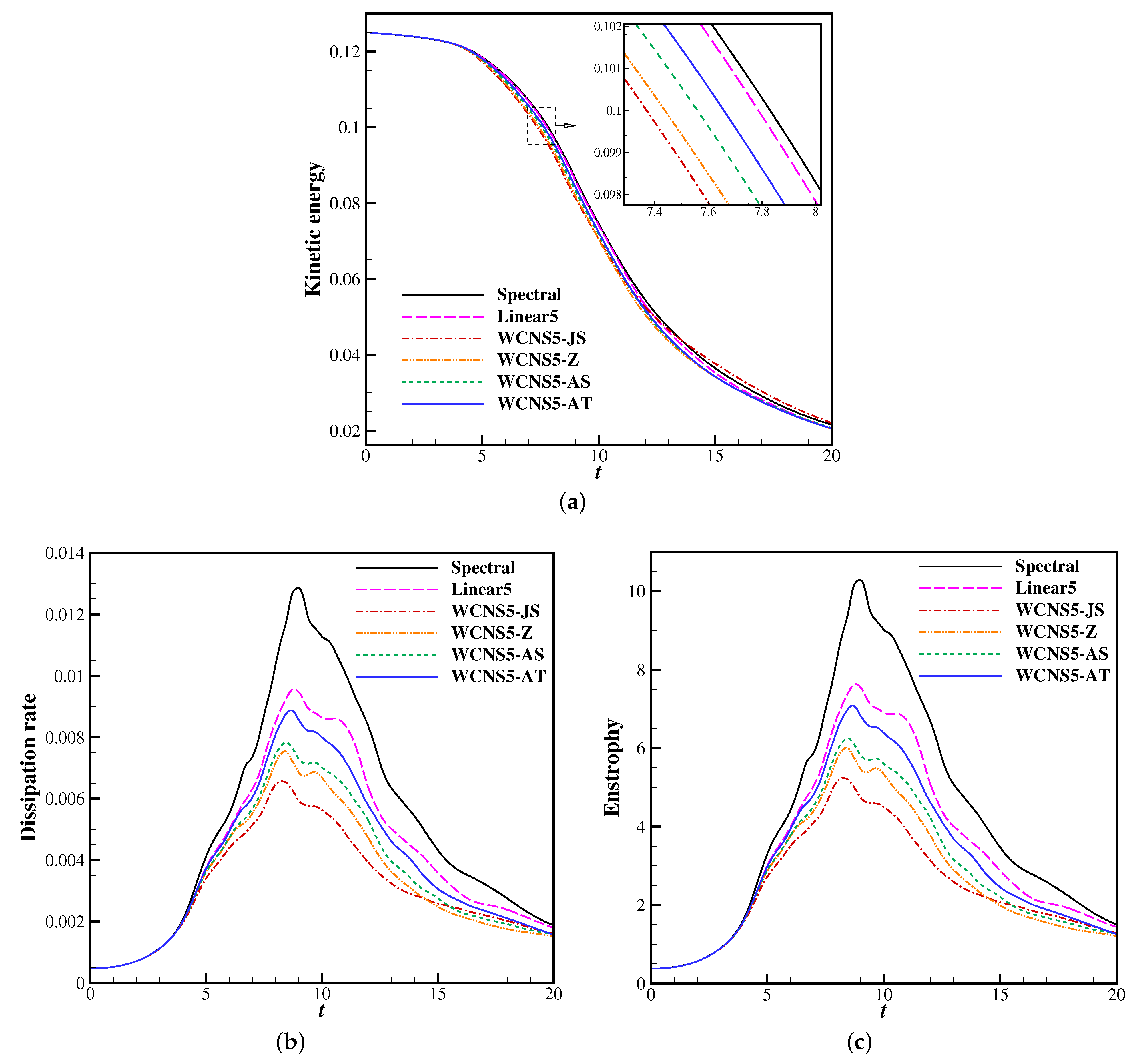
3.4. Three-Dimensional Navier–Stokes Equations

This section examines the performance of ${\widetilde{ϵ}}_{\mathrm{adp}}$ in three-dimensional Navier–Stokes equations by testing the viscous Taylor-Green vortex [40]. As a challenging example in the International Workshops on High-Order CFD Methods, the viscous Taylor-Green vortex is widely used to assess the resolution and numerical dissipation of schemes. The viscous terms are discretized using a sixth-order central explicit scheme. The computational domain is set as $x,y,z\in [-\pi ,\pi ]$, and the initial condition is as follows

$$\begin{array}{cc}\hfill u& =V_{0}sin\left(\frac{x}{L}\right)cos\left(\frac{y}{L}\right)cos\left(\frac{z}{L}\right),v=-V_{0}cos\left(\frac{x}{L}\right)sin\left(\frac{y}{L}\right)cos\left(\frac{z}{L}\right),\hfill \\ \hfill w& =0,p=p_0+\frac{{\rho }_0{V}_0^2}{16}\left(cos\left(\frac{2x}{L}\right)+cos\left(\frac{2y}{L}\right)\right)\left(cos\left(\frac{2z}{L}\right)+2\right)\hfill \end{array}$$

(45)

Periodic boundary conditions are imposed on the three directions. The Reynolds number is $\mathrm{Re}=1600$. The computation is advanced to $t=20t_c$ with $dt=5\times {10}^{-4}$, where $t_c$ and $dt$ are characteristic convective time and constant nondimensional time step, respectively. The remaining setup can be found in Ref. [41]. A uniform grid with $257\times 257\times 257$ points is used. Figure 21 presents the temporal evolutions of the kinetic energy, kinetic energy dissipation rate, and enstrophy, and the reference solution is given by the spectral method with $512\times 512\times 512$ grid points in Ref. [42]. For $t>4$, the statistics begin to deviate from the reference solution, and the results of the Linear5 scheme are more accurate due to smaller dissipation. The WCNS5-AT scheme gives the most accurate results compared with other nonlinear schemes, which indicates that the improvement of the dissipation and resolution for the JS weight function using ${\widetilde{ϵ}}_{\mathrm{adp}}$ is very significant.

3.5. Computational Efficiency

To demonstrate the advantages of ${\widetilde{ϵ}}_{\mathrm{adp}}$ more comprehensively, this section selects four representative numerical examples from the aforementioned tests to analyze the computational efficiency of ${\widetilde{ϵ}}_{\mathrm{adp}}$.

Table 3. CPU time (unit: s) and time increment (compared with the WCNS5-JS scheme).

Schemes	Composite Wave		Titarev-Toro		Double Mach		Viscous Taylor-Green Vortex
WCNS5-JS	4.896	-	13.259	-	272.297	-	298.975	-
WCNS5-Z	5.021	2.55%	14.078	6.17%	277.783	2.02%	299.995	0.34%
WCNS5-$\mathrm{AS}$	14.479	195.73%	25.744	94.16%	473.617	73.93%	364.610	21.95%
WCNS5-$\mathrm{AT}$	5.473	11.2%	14.343	8.17%	291.249	6.96%	303.341	1.46%

shows the computational time of different WCNS schemes and the increment in computational cost relative to the WCNS5-JS scheme. It should be noted that the computational time is averaged over five numerical tests, and the time of advancing 200 steps is recorded for the three-dimensional viscous Taylor-Green vortex example. It can be clearly drawn from Table 3 that the introduction of ${\widetilde{ϵ}}_{\mathrm{adp}}$ brings little computational increment to the JS weight function. Notice that this additional cost is further reduced as the dimension and scale of the problem increase. In addition, the new WCNS5-AT scheme is much more efficient than the WCNS5-AS scheme since the calculation of the standard deviation is omitted.

4. Conclusions

In this paper, we propose a new $ϵ$-adaptive algorithm for improving the fifth-order WCNS scheme. A high-order global smoothness indicator is introduced to increase $ϵ$ in smooth regions to improve resolution and accuracy, while decrease $ϵ$ near discontinuities to suppress numerical oscillations. The convergence accuracy at critical points is discussed in detail. The nonlinear mechanism treats high-order critical points as discontinuities due to excessive relative disparity in smoothness indicators, resulting in a loss of accuracy, which is solved by the new adaptive algorithm. A series of theoretical analyses and numerical tests are carried out, and following conclusions can be obtained

(1)

${\widetilde{ϵ}}_{\mathrm{adp}}$ helps the WCNS5-JS scheme recover spectral characteristics of the background linear scheme in the medium and low wavenumber range, and maintain design order at critical points by concealing the relative disparity in smoothness indicators.

(2)

${\widetilde{ϵ}}_{\mathrm{adp}}$ makes nonlinear schemes scale-invariant of flow variables, which yields consistent suppression for strong numerical oscillations near discontinuities caused by scaling down, thus improving the applicability and robustness of the WCNS scheme.

(3)

${\widetilde{ϵ}}_{\mathrm{adp}}$ significantly reduces nonlinear error in smooth regions, improves resolution for both complex small-scale flow structures and discontinuities, and further suppresses numerical oscillations, with a minor increment in computational cost.

To sum up, the well-balanced performance of the new adaptive algorithm makes it a good alternative for improving weighted schemes. It is worth noticing that ${\widetilde{ϵ}}_{\mathrm{adp}}$ can be easily extended to various WCNS/WENO schemes, which is left for future work.

References

- Harten, A. High Resolution Schemes for Hyperbolic Conservation Laws. J. Comput. Phys. 1997, 135, 260–278. [Google Scholar] [CrossRef] [Green Version]
- Liu, X.D.; Osher, S.; Chan, T. Weighted Essentially Non-oscillatory Schemes. J. Comput. Phys. 1994, 115, 200–212. [Google Scholar] [CrossRef] [Green Version]
- Jiang, G.S.; Shu, C.W. Efficient Implementation of Weighted ENO Schemes. J. Comput. Phys. 1996, 126, 202–228. [Google Scholar] [CrossRef] [Green Version]
- Henrick, A.K.; Aslam, T.D.; Powers, J.M. Mapped Weighted Essentially Non-Oscillatory Schemes: Achieving Optimal Order near Critical Points. J. Comput. Phys. 2005, 207, 542–567. [Google Scholar] [CrossRef]
- Borges, R.; Carmona, M.; Costa, B.; Don, W.S. An Improved Weighted Essentially Non-Oscillatory Scheme for Hyperbolic Conservation Laws. J. Comput. Phys. 2008, 227, 3191–3211. [Google Scholar] [CrossRef]
- Don, W.S.; Borges, R. Accuracy of the Weighted Essentially Non-Oscillatory Conservative Finite Difference Schemes. J. Comput. Phys. 2013, 250, 347–372. [Google Scholar] [CrossRef]
- Wang, R.; Feng, H.; Huang, C. A New Mapped Weighted Essentially Non-oscillatory Method Using Rational Mapping Function. J. Sci. Comput. 2016, 67, 540–580. [Google Scholar] [CrossRef]
- Acker, F.; Borges, R.D.; Costa, B. An Improved WENO-Z Scheme. J. Comput. Phys. 2016, 313, 726–753. [Google Scholar] [CrossRef]
- Luo, X.; Wu, S.P. An Improved WENO-Z+ Scheme for Solving Hyperbolic Conservation Laws. J. Comput. Phys. 2021, 445, 110608. [Google Scholar] [CrossRef]
- Castro, M.; Costa, B.; Don, W.S. High Order Weighted Essentially Non-Oscillatory WENO-Z Schemes for Hyperbolic Conservation Laws. J. Comput. Phys. 2011, 230, 1766–1792. [Google Scholar] [CrossRef]
- Musa, O.; Huang, G.; Wang, M. A New Smoothness Indicator of Adaptive Order Weighted Essentially Non-Oscillatory Scheme for Hyperbolic Conservation Laws. Mathematics 2021, 9, 69. [Google Scholar] [CrossRef]
- Shen, Y.; Zha, G.; Wang, B. Improvement of Stability and Accuracy for Weighted Essentially Nonoscillatory Scheme. AIAA J. 2009, 47, 331–344. [Google Scholar] [CrossRef]
- Yamaleev, N.K.; Carpenter, M.H. A Systematic Methodology for Constructing High-Order Energy Stable WENO Schemes. J. Comput. Phys. 2009, 228, 4248–4272. [Google Scholar] [CrossRef] [Green Version]
- Hu, X.; Adams, N. Scale Separation for Implicit Large Eddy Simulation. J. Comput. Phys. 2011, 230, 7240–7249. [Google Scholar] [CrossRef]
- Aràndiga, F.; Martí, M.C.; Mulet, P. Weights Design For Maximal Order WENO Schemes. J. Sci. Comput. 2014, 60, 641–659. [Google Scholar] [CrossRef]
- Peer, A.; Dauhoo, M.; Bhuruth, M. A Method for Improving the Performance of the WENO5 Scheme near Discontinuities. Appl. Math. Lett. 2009, 22, 1730–1733. [Google Scholar] [CrossRef] [Green Version]
- Jia, F.; Gao, Z.; Don, W.S. A Spectral Study on the Dissipation and Dispersion of the WENO Schemes. J. Sci. Comput. 2015, 63, 49–77. [Google Scholar] [CrossRef]
- Zheng, S.; Deng, X.; Wang, D.; Xie, C. A Parameter-free ε-adaptive Algorithm for Improving Weighted Compact Nonlinear Schemes. Int. J. Numer. Methods Fluids 2019, 90, 247–266. [Google Scholar] [CrossRef]
- Deng, X.; Maekawa, H. Compact High-Order Accurate Nonlinear Schemes. J. Comput. Phys. 1997, 130, 77–91. [Google Scholar] [CrossRef]
- Deng, X.; Zhang, H. Developing High-Order Weighted Compact Nonlinear Schemes. J. Comput. Phys. 2000, 165, 22–44. [Google Scholar] [CrossRef]
- Wang, D.; Deng, X.; Wang, G.; Dong, Y. Developing a Hybrid Flux Function Suitable for Hypersonic Flow Simulation with High-Order Methods. Int. J. Numer. Methods Fluids 2016, 81, 309–327. [Google Scholar] [CrossRef]
- Deng, X.; Mao, M.; Tu, G.; Liu, H.; Zhang, H. Geometric Conservation Law and Applications to High-Order Finite Difference Schemes with Stationary Grids. J. Comput. Phys. 2011, 230, 1100–1115. [Google Scholar] [CrossRef]
- Deng, X.; Min, Y.; Mao, M.; Liu, H.; Tu, G.; Zhang, H. Further Studies on Geometric Conservation Law and Applications to High-Order Finite Difference Schemes with Stationary Grids. J. Comput. Phys. 2013, 239, 90–111. [Google Scholar] [CrossRef]
- Deng, X.; Liu, X.; Mao, M.; Zhang, H. Investigation on Weighted Compact Fifth-Order Nonlinear Scheme and Applications to Complex Flow. In Proceedings of the 17th AIAA Computational Fluid Dynamics Conference, Toronto, ON, Canada, 6–9 June 2005; American Institute of Aeronautics and Astronautics: Toronto, ON, Canada, 2005. [Google Scholar] [CrossRef]
- Sun, X.W.; Yang, X.L.; Liu, W. Aero-Optical and Aero-Heating Effects of Supersonic Turbulent Boundary Layer with a Tangential Wall-Injection Film. Phys. Fluids 2021, 33, 035118. [Google Scholar] [CrossRef]
- Nonomura, T.; Fujii, K. Effects of Difference Scheme Type in High-Order Weighted Compact Nonlinear Schemes. J. Comput. Phys. 2009, 228, 3533–3539. [Google Scholar] [CrossRef]
- Yan, Z.; Liu, H.; Mao, M.; Zhu, H.; Deng, X. New Nonlinear Weights for Improving Accuracy and Resolution of Weighted Compact Nonlinear Scheme. Comput. Fluids 2016, 127, 226–240. [Google Scholar] [CrossRef]
- Pirozzoli, S. On the Spectral Properties of Shock-Capturing Schemes. J. Comput. Phys. 2006, 219, 489–497. [Google Scholar] [CrossRef]
- Hu, X.Y.; Tritschler, V.K.; Pirozzoli, S.; Adams, N.A. Dispersion-Dissipation Condition for Finite Difference Schemes. arXiv 2014, arXiv:1204.5088. [Google Scholar]
- Steger, J.L.; Warming, R.F. Flux Vector Splitting of the Inviscid Gasdynamic Equations with Application to Finite-Difference Methods. J. Comput. Phys. 1981, 40, 263–293. [Google Scholar] [CrossRef]
- Gottlieb, S.; Shu, C.W.; Tadmor, E. Strong Stability-Preserving High-Order Time Discretization Methods. SIAM Rev. 2001, 43, 89–112. [Google Scholar] [CrossRef]
- Lax, P.D. Weak Solutions of Nonlinear Hyperbolic Equations and Their Numerical Computation. Commun. Pure Appl. Math. 1954, 7, 159–193. [Google Scholar] [CrossRef]
- Sod, G.A. A Survey of Several Finite Difference Methods for Systems of Nonlinear Hyperbolic Conservation Laws. J. Comput. Phys. 1978, 27, 1–31. [Google Scholar] [CrossRef] [Green Version]
- Shu, C.W.; Osher, S. Efficient Implementation of Essentially Non-Oscillatory Shock-Capturing Schemes, II. J. Comput. Phys. 1989, 83, 32–78. [Google Scholar] [CrossRef]
- Titarev, V.A.; Toro, E.F. Finite-Volume WENO Schemes for Three-Dimensional Conservation Laws. J. Comput. Phys. 2004, 201, 238–260. [Google Scholar] [CrossRef]
- Balsara, D.S.; Shu, C.W. Monotonicity Preserving Weighted Essentially Non-oscillatory Schemes with Increasingly High Order of Accuracy. J. Comput. Phys. 2000, 160, 405–452. [Google Scholar] [CrossRef] [Green Version]
- Lax, P.D.; Liu, X.D. Solution of Two-Dimensional Riemann Problems of Gas Dynamics by Positive Schemes. SIAM J. Sci. Comput. 1998, 19, 319–340. [Google Scholar] [CrossRef] [Green Version]
- Shi, J.; Zhang, Y.T.; Shu, C.W. Resolution of High Order WENO Schemes for Complicated Flow Structures. J. Comput. Phys. 2003, 186, 690–696. [Google Scholar] [CrossRef] [Green Version]
- Woodward, P.; Colella, P. The Numerical Simulation of Two-Dimensional Fluid Flow with Strong Shocks. J. Comput. Phys. 1984, 54, 115–173. [Google Scholar] [CrossRef]
- Brachet, M.E.; Meiron, D.I.; Orszag, S.A.; Nickel, B.G.; Morf, R.H.; Frisch, U. Small-Scale Structure of the Taylor–Green Vortex. J. Fluid Mech. 1983, 130, 411. [Google Scholar] [CrossRef] [Green Version]
- Zheng, S.; Deng, X.; Wang, D. New Optimized Flux Difference Schemes for Improving High-Order Weighted Compact Nonlinear Scheme with Applications. Appl. Math. Mech. 2021, 42, 405–424. [Google Scholar] [CrossRef]
- van Rees, W.M.; Leonard, A.; Pullin, D.I.; Koumoutsakos, P. A Comparison of Vortex and Pseudo-Spectral Methods for the Simulation of Periodic Vortical Flows at High Reynolds Numbers. J. Comput. Phys. 2011, 230, 2794–2805. [Google Scholar] [CrossRef]