Article

A Passivity-Based Velocity Control Method of Hardware-in-the-Loop Simulation for Space Robotic Operations

School of Mechanical Engineering, Shanghai Jiao Tong University, Shanghai 200240, China
*
Author to whom correspondence should be addressed.
Aerospace 2022, 9(7), 368; https://doi.org/10.3390/aerospace9070368
Submission received: 22 April 2022 / Revised: 13 June 2022 / Accepted: 7 July 2022 / Published: 8 July 2022
(This article belongs to the Section Astronautics & Space Science)

Abstract

:
The hardware-in-the-loop (HIL) simulation is an important approach to test space robotic operations, rendering virtual free-floating dynamics on robotic facilities. However, this approach suffers from velocity divergence due to intrinsic time delay in the control loop. This paper proposes a passivity-based control strategy to handle the simulation divergence. A HIL simulation system with an industrial robot is modelled and its divergence problems are analyzed through numerical simulations. Then, through representing the HIL simulation system in a passivity network of view, the passivity observer (PO) of the dynamic system is established. The PO includes the effect of a real contact damping on energy flow of the passivity network during a contact process. Thus, a passivity controller is defined. Moreover, a real-time estimation method for contact damping is presented. Finally, collision experiments against a virtual wall and real collision experiments are both implemented. The experimental results show that the simulation divergence due to the time delay can be prevented by the proposed control strategy, and that the velocity characteristics with high fidelity are rendered on the HIL simulation system.

1. Introduction

Space robotic operations play a key role in future space missions, such as the removal of space debris in orbit and maintenance tasks on defected satellites [1,2]. These robotic operations all require intensive simulations on the ground in order to validate robotic mechanisms and control strategies in space. Thus, it is of utmost importance to reproduce zero-gravity conditions on the ground. Within this context, there are three categories of simulation technologies, namely full numerical simulations, full physical simulations, and hybrid simulations [3]. The full numerical simulation adopts a software to emulate a space dynamic process, which is a low-cost approach. However, it is not suitable for rendering multiple degrees-of-freedom (DOFs) manipulations because its accuracy depends on mathematical models with unknown physical parameters [4]. The second category includes air-bearing-based testbeds [5,6], water-based neutral buoyancy [7], and parabolic flights [8]. These approaches are usually expensive and not flexible on the changes in simulation parameters. The hybrid simulation, which is also referred to as hardware-in-the-loop (HIL) simulation, combines hardware tests with software simulation. This approach has both merits of high flexibility and accuracy, being an attractive approach for simulating complicated robotic tasks in space [1,3].
Many HIL simulators have been developed for the verification of space robotic operations. Shimoji et al. [9] proposed the first HIL simulator, which consisted of a multi-DOF docking-mimicking mechanism, a 5-DOF translational target, and simulation software. Mitchell et al. [10] in the Johnson Space Center presented a 6-DOF parallel robotic facility (SDTS) to simulate rendezvous and docking (RvD) processes. Takhashi et al. [11] presented a 9-DOF hybrid simulator, which consists of a 2-DOF translational table, a 6-DOF parallel robot and 1-DOF spin motion table. In addition, a dual-manipulator-based HIL system has been developed for simulating capturing operations [12]. The Canada Space Agency (CSA) has also developed a dual manipulator HIL system for the entire dynamic process of capturing a tumbling satellite [13]. The German Aerospace Center (DLR) adopted two industrial robots to emulate the 6-DOF dynamic maneuvering of two satellites [14], which has been used for the Deutsche Orbitale Servicing Mission (DEOS) and On-orbit Servicing (OOS) missions [15]. Recently, Gao et al. [16] presented a novel 9-DOF HIL simulation system. A pair of docking mechanisms are mounted on a 3-DOF parallel robot and a 6-DOF parallel robot, respectively. The 3-DOF parallel robot consists of three limbs with prismatic-revolute-spherical (PRS) joints. Its prismatic joints are active and their ranges of motion reach up to three meters. Thus, the simulator is capable of simulating the final approaching process.
A crucial question for the HIL simulation is how to handle the simulation distortion due to an intrinsic time delay [17]. The time delay exists inevitably between the measured signals and the simulation-driven response of the simulator; thus, the stability of the HIL simulation system will be disrupted [18]. The time delay comes from two aspects. One is the fixed time delay, such as a sampling time for force measurement. The fixed time delay can be compensated by a phase lead model [2]. The other is the dynamic response delay of the robotic simulator, which is difficult to be modelled, owing to the tremendous complexity of a robotic facility. In order to reduce the dynamic response delay as far as possible, some existing HIL simulation systems [10,11,16] have adopted parallel kinematic mechanisms (PKMs) with higher rigidity and better dynamic characteristics than their serial counterparts [19]. However, the improvement of dynamic characteristics cannot thoroughly eliminate the simulation divergence.
Since it is difficult to obtain the exact dynamic parameters of robotic simulators, some model-free control strategies have been developed to guarantee the stability of the simulation. One category of ideas is to directly establish a response error model of the end-effector of the simulator. A first-order compensation model has been implemented to the HIL simulation control [20]. Furthermore, Qi et al. [2] designed a second-order filter model based force compensation; thus, the dynamic response model of the simulator is not required. The other category is based on the passivity of a free-floating dynamic system in space. The passivity theory derives from classic mechanics [21] and was extended to motion control fields [22]. In particular, for adaptive control of robots, the passivity control method has been investigated widely [23,24]. The main issue of the passivity approach is that it is over-conservative because its close-loop performance depends on a so-called damping factor [25]. The virtual damping is used to dissipate the energy generated in a dynamic process. However, if fixed damping was used for the control, the performance could be poor for many cases [26]. Hannaford and Ryu [27] proposed a novel idea of variable damping based on a time-domain passivity controller (PC) for a two-port passivity network to ensure the stability of a dynamic system. This approach has been successfully used for teleoperation control [26] and haptic interfaces [27]. Recently, Marco et al. [28] creatively proposed a passivity-based control strategy to solve the simulation distortion due to both time delay and discrete-time integration in a HIL simulation system based two industrial robots.
All the above studies provide a solid foundation for the present research on the control strategy of a HIL simulation system. The end-effector of the HIL simulator can achieve a stable velocity performance through the virtual damping based on the PC. The rebounding velocity after each collision is almost equal to the initial contact velocity. However, the physical meanings of the virtual damping and compensation parameters were still not clarified in earlier studies. In fact, the energy is undoubtedly decreased due to damping dissipation in a real contact dynamic process. To obtain the stable velocity performance, force performance is inevitably sacrificed. A possible method is to identify the real contact damping in real time during the HIL simulation. The estimated damping can be used to distinguish the damping force from the elastic force in a space contact process. Since the work carried out by the damping force is just the dissipated energy, the practical contact process including energy dissipation can be rendered on the HIL simulator. Moreover, the energy increase due to time delay can be prevented.
The contribution of this paper is to propose a passivity-based control strategy for solving velocity divergence of a HIL simulation system due to time delay. This approach provides the virtual damping of a traditional PC with an exact physical meaning by means of the real-time identification of contact damping. A HIL simulation system with an industrial robot is modelled and its existing problems due to time delay are analyzed through numerical simulations. Then, the passivity control method based on damping estimation is proposed. Finally, the experiments are implemented and the results validate the proposed method. The remainder of this paper is organized as follows. The HIL simulation system is introduced in Section 2. The control method is proposed in Section 3. Section 4 gives the experiment and discussion. Finally, conclusions are given in Section 5.

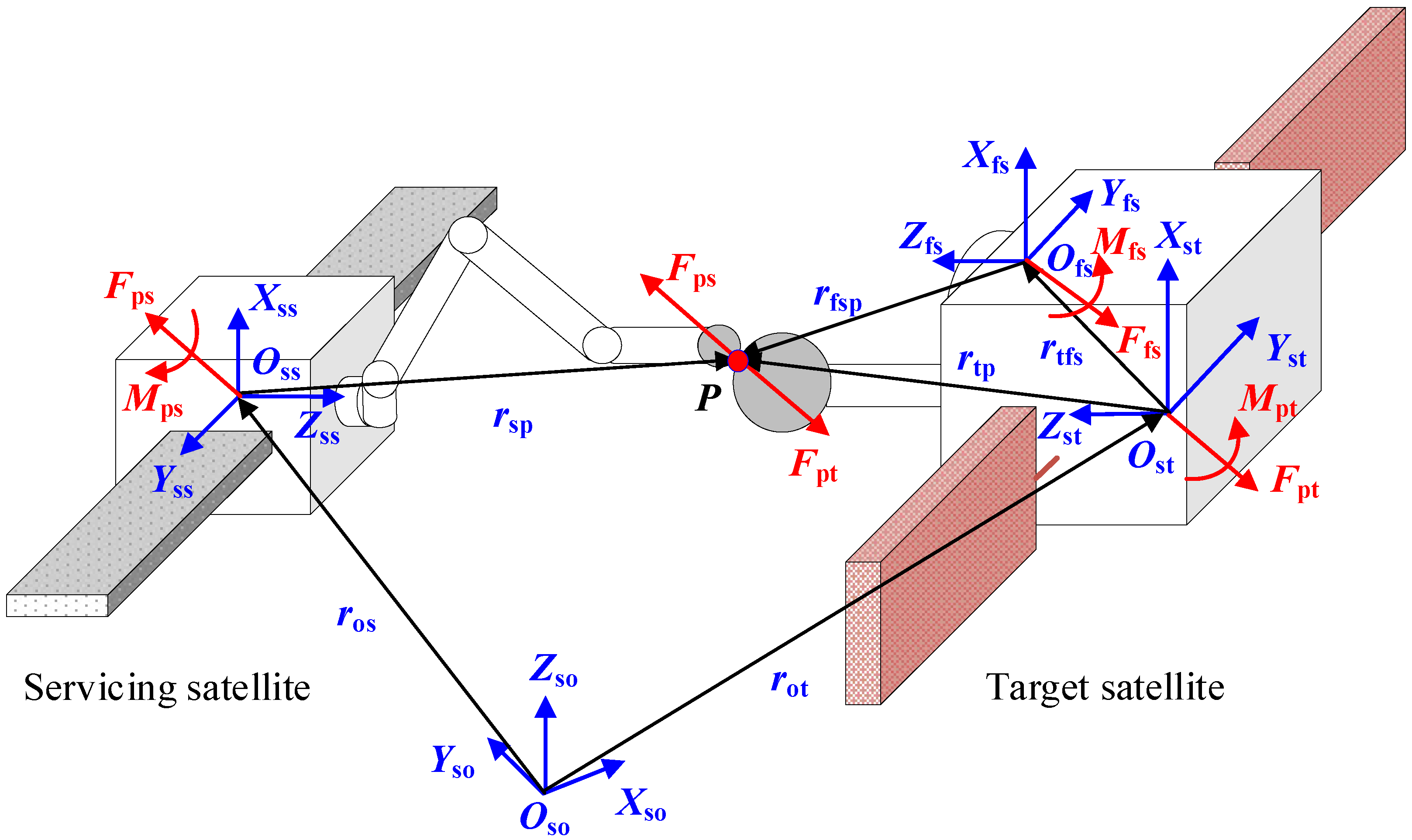
2. Modelling of the HIL Simulation System

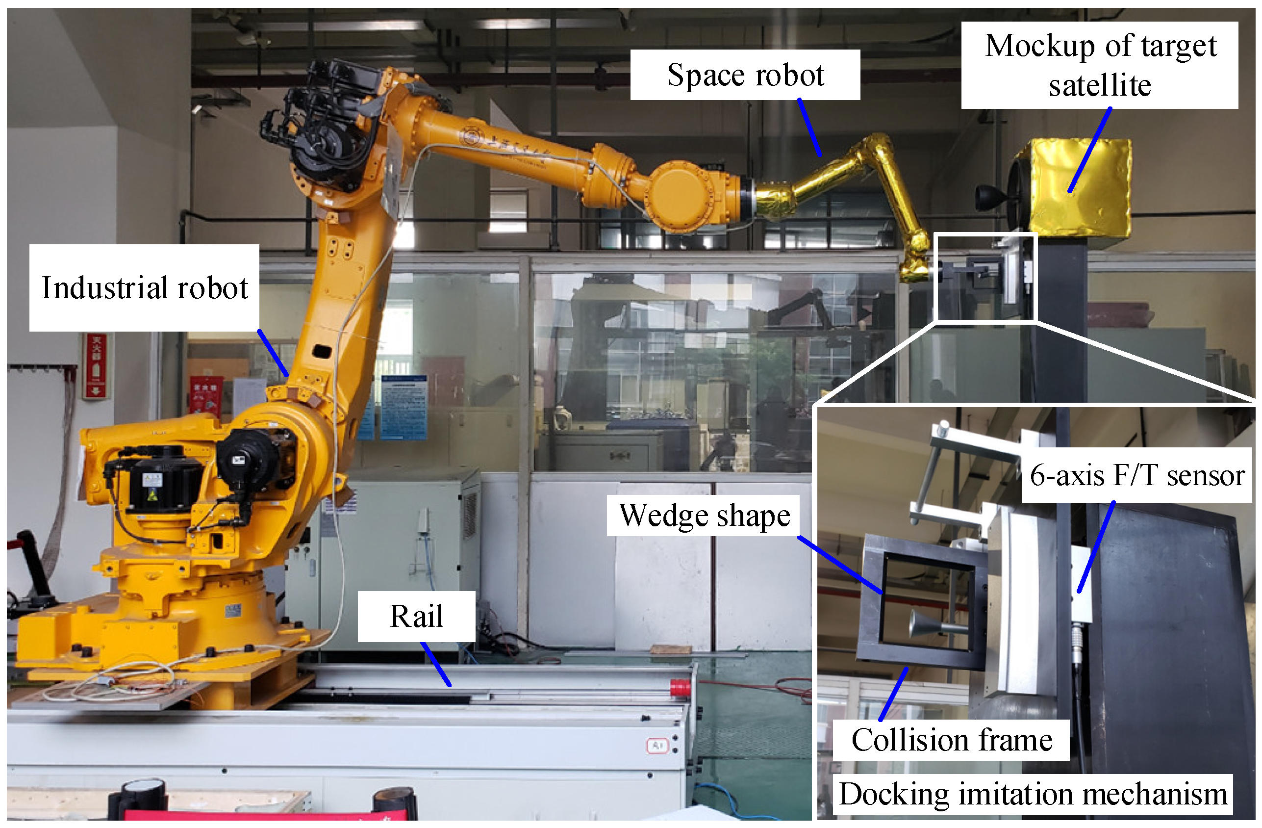
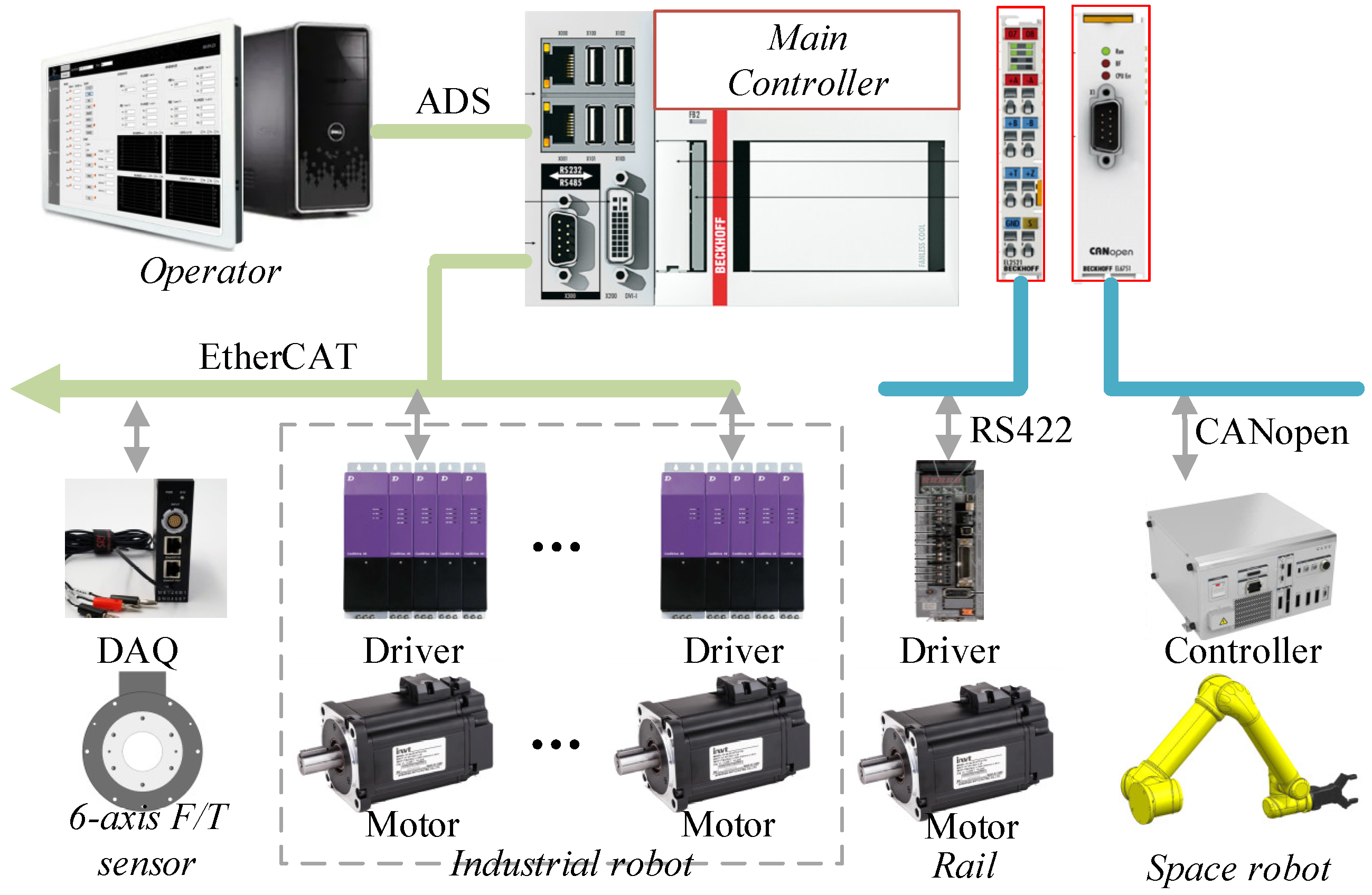
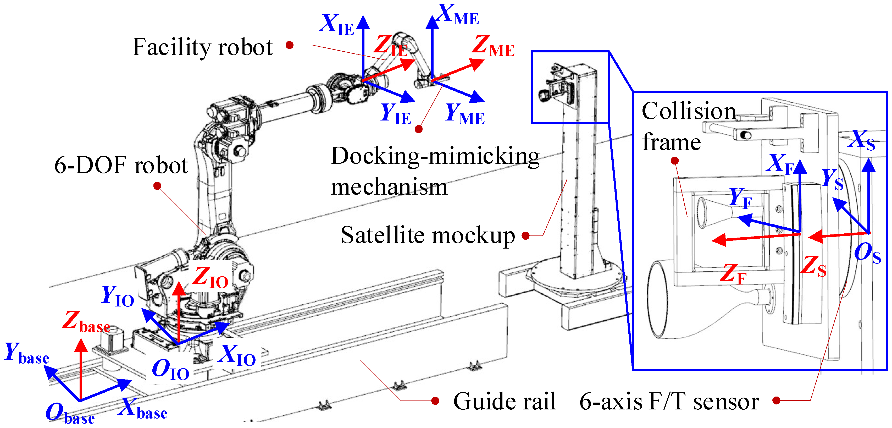
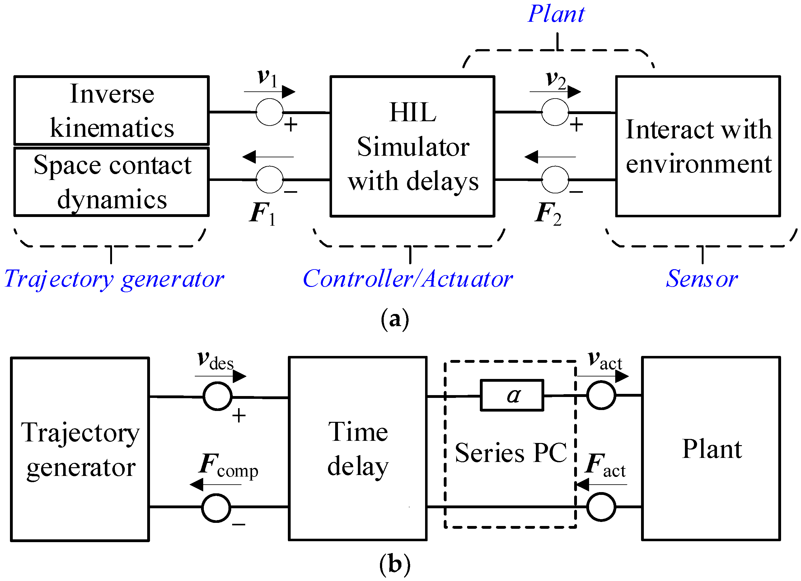
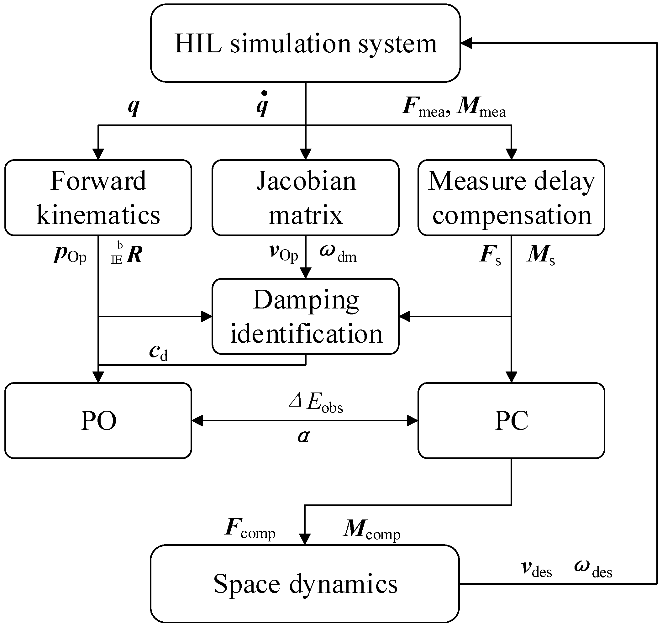
2.1. The HIL Simulation System

To simulate the free-floating dynamics, a HIL simulator using a 6-DOF industrial robot is proposed, as observed in Figure 1. The mechanical system consists of an industrial robot, a facility robot, a guide rail, a pair of docking-mimicking mechanisms, a satellite mockup, and a 6-axis force/torque (F/T) sensor. The industrial robot is mounted on the guide rail to extend the translational range of the simulator. The docking imitation mechanisms are designed as a collision rod and a collision frame. To produce a point contact between the frame and the rod, the wedge-shaped inner sides of the collision frame are fabricated. The facility robot with the collision rod is installed on the end-effector of the industrial robot. The 6-axis F/T sensor is between the collision frame and the satellite mockup. The specifications of the HIL simulation system are shown in Table 1.
The control hardware of the HIL simulation system is shown in Figure 2. A main controller was adopted to run the entire control program. The control software was developed using the TwinCAT software platform, a real-time PC-based control system from Beckhoff company. The main controller communicates with six servo drives of the industrial robot and a six-axis F/T sensor in real time via the EtherCAT industrial network protocol. In addition, the main controller communicates with the drive of the rail and the space robot by means of the RS-422 serial data standard and CANopen protocol, respectively.
The control approach for realizing a zero-gravity environment is shown in Figure 3. There is a hardware layer and a software layer. The hardware layer consists of the industrial robot, the space robot, and the 6-axis F/T sensor. The software layer includes a kinematics module, a motion control subsystem, a free-floating dynamics module, and a time-delay compensation module. The free-floating dynamics module receives the collision force from the 6-axis F/T sensor, and then yields the desired motion trajectory of the simulator. After that, the HIL simulator can emulate the satellite motion process in Cartesian space through the kinematics module. However, there is a time delay between the measured force and the position sent to the robot. The time delay comes from two aspects, namely a dynamic response delay from the industrial robot and a fixed delay from the measurement system. If there is no compensation control, the measured force is directly sent to the free-floating dynamics module, as observed in the blue flow chart of Figure 3. As aforementioned, the time delay will lead to simulation divergence [3,17]. Therefore, it is necessary to propose a compensation module. The kinematics module and the free-floating dynamics module are illustrated in this section and the detailed compensation module will be given in Section 3.

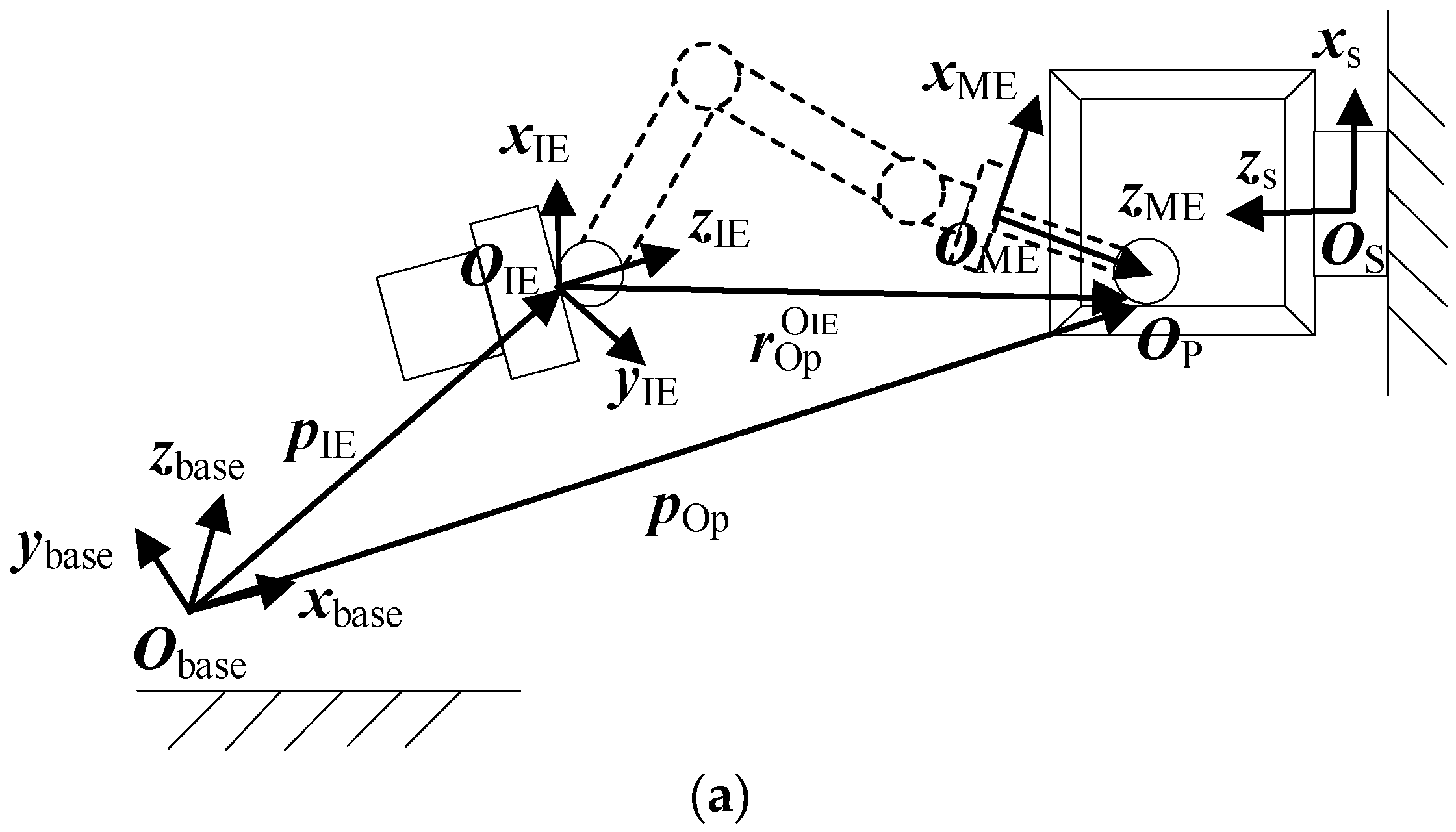
2.2. Kinematics of the Simulator

The coordinate systems of the HIL simulator are established, as observed in Figure 4. {Obase} is the global coordinate system; {OIO} and {OIE} are the base coordinate system and the end-effector coordinate system of the industrial robot, respectively; {OME} is the assembly coordinate system on the simulator of the servicing satellite; {OF} is the assembly coordinate system on the mockup of the target satellite; {OS} is the coordinate system of the F/T sensor.
For the industrial robot, the Denavit–Hartenberg (D-H) coordinate systems can be established and thus the D-H matrices are adopted to describe the forward kinematics of the robot. The transformation matrix from frame i to i − 1 for the ith limb can be written as
T i i 1 = [ c θ i s θ i c α i s θ i s α i a i c θ i s θ i c θ i c α i c θ i s α i a i s θ i 0 s α i c α i d i 0 0 0 1 ]
where s and c denote the sine and cosine functions. Therefore, the forward kinematics of the robot is described as
T 6 0 = T 1 0 T 2 1 T 6 5 ,
where the coordinate system {O0-x0y0z0} and the {OIO} coincide; {O6-x6y6z6} and {OIE} coincide. Since the industrial robot includes three consecutive axes that intersect at a point, it is well-known that this kind of robot has a closed-form solution. The detailed inverse kinematics can be found in [29].

2.3. Free-Floating Dynamics

Space contact dynamics is a complex full 3-D collision physical process. Compared with the satellites, docking mechanisms or robotic operation tools have significantly smaller sizes. The physical contact that results in robotic operations can be regarded as a point contact. Thus, there is only contact force between the docking mechanisms. Without considering the friction, the contact force occurs along the normal of the contact surface. Accordingly, the full collision can be regarded as a 1-D collision along the resultant force at the contact point.
Figure 5 shows coordinate systems of two free-floating satellites. {Oso} is the global coordinate of the satellite system, which corresponds to the {Obase} in Figure 1. {Oss} and {Ost} are the coordinate systems at the centers of mass (CoMs) of two satellites, respectively. The relative relationship between the {Oss} and the {Ost} systems corresponds to the {OIE} in Figure 4. {Ofs} is the coordinate sytem of the F/T sensor, which corresponds to {OS}. In addition, force analysis during space robotic operations is also depicted in Figure 3. After the space robot on the servicing satellite operates the target satellite, there exists a pair of contact force, Fps and Fpt. The contact force can be measured by the F/T sensor. Thus, the force and moment applied on the center of mass (CoM) of the satellite, Fps and Mps, Fpt and Mpt, can be obtained. Substituting them into the following free-floating dynamic equations leads to the desired motion trajectories of the satellites.
The translational dynamics of a free-floating satellite can be denoted by
v ( t ) = 0 t F c ( t ) M d t ,
and the rotational dynamics is written as
ω ( t ) = 0 t I 1 [ τ C ( t ) ω ( t ) × I ω ( t ) ] d t ,
where F C ( t ) 3 × 1 and τ C ( t ) 3 × 1 are the forces and moments applied on the center of mass (CoM) of the satellite, respectively; v ( t ) 3 × 1 and ω ( t ) 3 × 1 are the linear velocity of the CoM and the angular velocity of the satellite; M is the mass of the satellite and I 3 × 3 is the inertia matrix of the satellite, with respect to the coordinate system at the CoM.
The 6-axis T/T sensor is usually adopted to measure the contact force and moment. Thus, to describe the force wrench in regard to the CoM frame, the following transformations are given by
F C = R s c F s ,
τ C = r c , s × ( R s c F s ) + R s c τ s ,
where R s c is the rotation matrix between the sensor frame and the CoM frame; rc,s is the vector from the origin of the sensor frame to the origin of the CoM frame; Fs and τs are the measured force and moment after measurement compensation, respectively.

3. Methodology

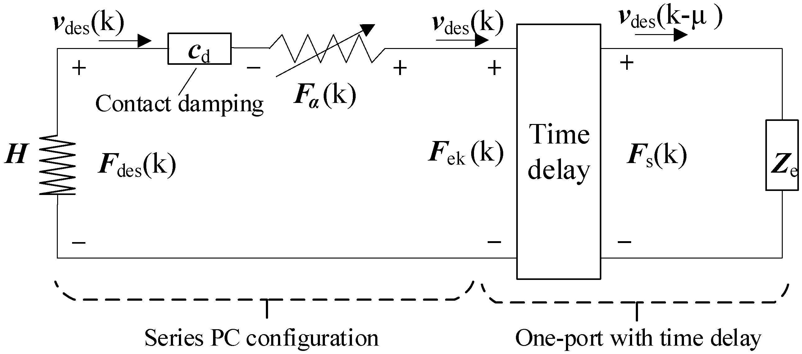
3.1. Passive Network

The traditional control system view of a HIL simulation system consists of the trajectory generator, the controller/actuator, the sensor, and the plant, as observed in Figure 6a. Since there is a response delay for the HIL simulator, the robot interacts with the environment with a delayed velocity v2. After each collision, the trajectory generator also obtains a delayed force, owing to the measurement delay of the 6-axis F/T sensor. According to the passivity theory, a traditional control view can be analyzed in terms of energy flow through representing it in a network point of view, as depicted in Figure 6b. The virtual energy flow can be described using a conjugate pair, such as force and velocity, voltage and current. Energy is written as the integral of inner product between the conjugate input and output [25]. Note that the ‘Energy’ may or may not correspond to a real physical energy. The main idea of a passivity-based control is to observe the energy flow through a passivity observer (PO) in real time and to dissipate the energy produced owing to the time delay through a passivity controller (PC).

3.2. PO and PC

One must consider a dynamic system with one power port [ F ( τ ) , v ( τ ) ] n × n (right-side of Figure 7), which energetically interacts with the environment. F(τ) and v(τ) are force-like and velocity-like variables, respectively. Note that the conjugate variables [ F ( τ ) , v ( τ ) ] in the HIL control system are discrete-time values.
According to definition of the passivity [25], with initial energy storage E(0) is passive if and only if,
E ( k ) = E ( 0 ) + i = 0 k F T ( k ) v ( k ) T sam ,
where Tsam is the sampling time.
Equation (7) means that the energy applied to a passive system must be positive all the time. If E(k) < 0, is producing energy and then the dynamic system becomes unstable. Moreover, the amount of the produced energy is −E(k). Since the exact value of energy generated is known, a time-varying element can be defined to dissipate the energy produced. This variable element is called a PC. There are serial or parallel configurations for the PC design. An admittance PC requires the dynamics of the industrial robot. However, the dynamics of an industrial robot is usually unknown. Thus, a series configuration with an impedance causality is adopted for the PC on the left-side of Figure 7.
Because there is a time delay, the robotic simulator interacts with the environment with a delayed velocity vdes(k − μ), which produces a force vdes(k − μ)Ze. Here, Ze is a damping-like variable. In addition, there is also contact damping dissipation between the imitation docking mechanisms. Accordingly, the energy flow can be calculated and the PO can be defined.
The PO of is the energy flow through the power port [ F ( k ) , v ( k ) ] at each time-step, which is given by
E obs ( k ) = E ( 0 ) + i = 0 k { F ek T ( k ) v des ( k ) T sam + F α T ( k 1 ) v des ( k 1 ) T sam } ,
F ek ( k ) = { F s ( k 1 ) c d ( k 1 ) v des ( k 1 ) , v des T ( k ) F s ( k ) > 0 F s ( k ) c d ( k ) v des ( k ) , v des T ( k ) F s ( k ) 0 ,
where Fek(k) is the elastic contact force; Fs(k) is the force after the measurement compensation, defined in Equation (10); Fα is the PC compensation force; cd is the contact damping. The identification method of cd will be given in the following subsection. In addition to the time delay, the discrete-integration degrades the behavior of the free-floating dynamics [28]. The work carried out by a rebound force during the acceleration process is larger than the work carried out by a resistance force during the deceleration process, owing to the mismatching of the integration steps of two stages. Therefore, to decrease the effect of the discrete-time integration on velocity divergence, Equation (9) calculates separately the elastic forces during the acceleration and deceleration stages.
As aforementioned, there is a fixed time delay for a 6-axis F/T sensor. The time delay can be described by a first-order model with a delay time τm as follows:
{ F s ( k ) = L 1 [ G ( s ) ] · F mea ( k ) M s ( k ) = L 1 [ G ( s ) ] · M mea ( k ) ,
where Fmea(k) and Mmea(k) are the force and moment measured by the sensor; G(s) = 1 + τms and L−1[G(s)] is the inverse Laplace transformation.
For a multi-DoF dynamic system, the energy produced needs be dissipated in the Cartesian space of a robot. Therefore, the energy Eobs(k) is decomposed into three coordinate axis directions according to the measured force, which is written as
E obs , i ( k ) = E obs ( k ) · F s , i ( k ) F s ( k ) , i = 1 , 2 , 3 ,
For multi-DOF contact in space, since the directions of vdes and Fek are not the same, the projection of the desired contact velocity to the contact force is used to calculate the PC compensation force, which is denoted by
F α ( k ) = v des T ( k ) F ek ( k ) F ek ( k ) 2 α ( k ) F ek ( k ) ,
where α ( k ) 3 × 1 is the time-varying damping matrix with a diagonal form, and α(k) = diag[α11(k), α22(k), α33(k)]. Evidently, if Eobs,i(k) < 0, to dissipate the energy generated at each step, the components of the damping matrix are given by
α i , i ( k ) = E obs , i ( k ) v des T ( k ) F ek ( k ) F ek ( k ) 2 F ek , i ( k ) v des , i ( k ) T sam , i = 1 , 2 , 3 ,
Similarly, since the moment measured by the sensor can be calculated by the contact force at the contact point, the PC compensation moment is written as
M α ( k ) = r fsp × F α ( k ) ,
where r fsp is the vector from the origin of the sensor coordinate system to the contact point.
Accordingly, the force and moment compensated by the PC, i.e., the inputs of the space dynamics, are denoted by
{ F comp ( k ) = F s ( k ) + F α ( k ) M comp ( k ) = M s ( k ) + M α ( k ) .

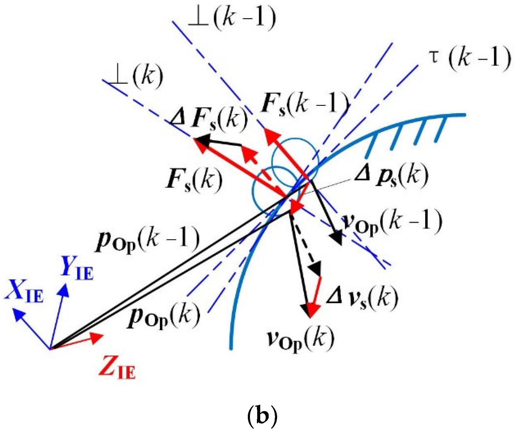
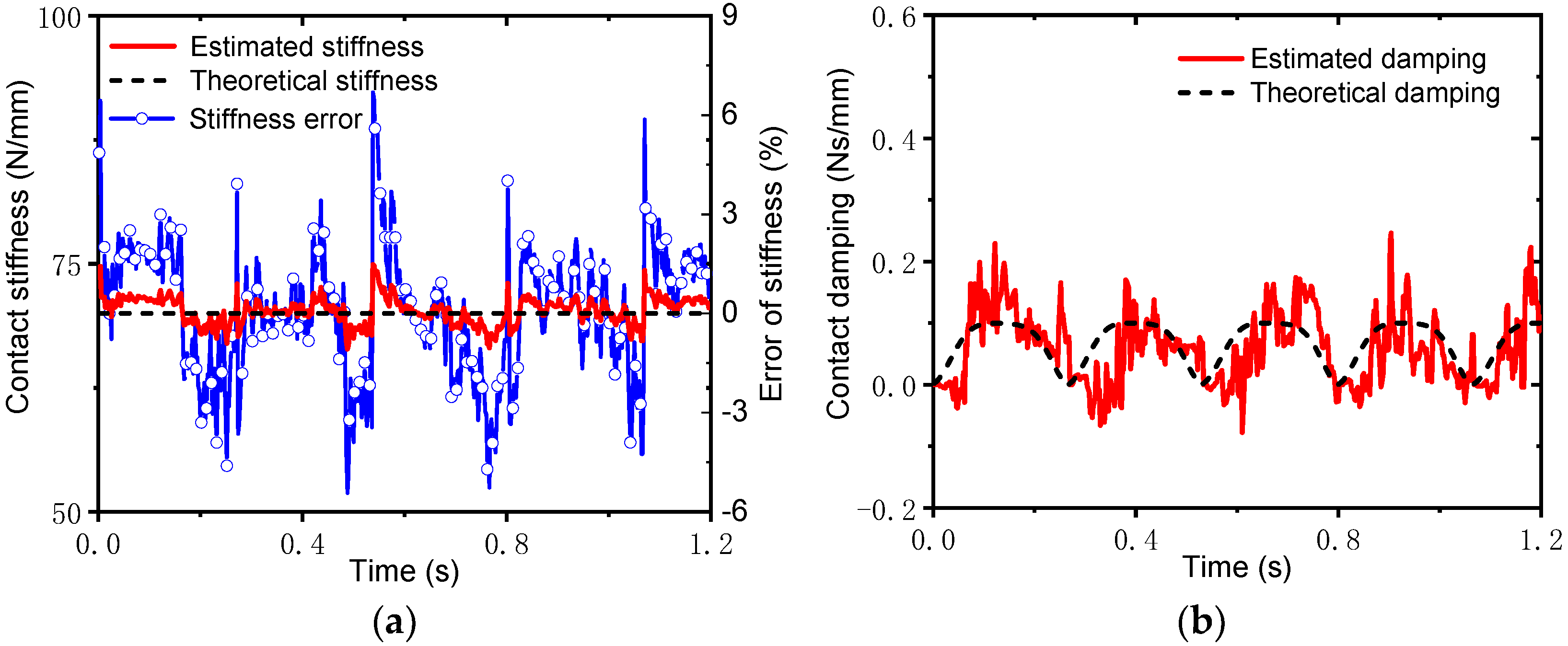
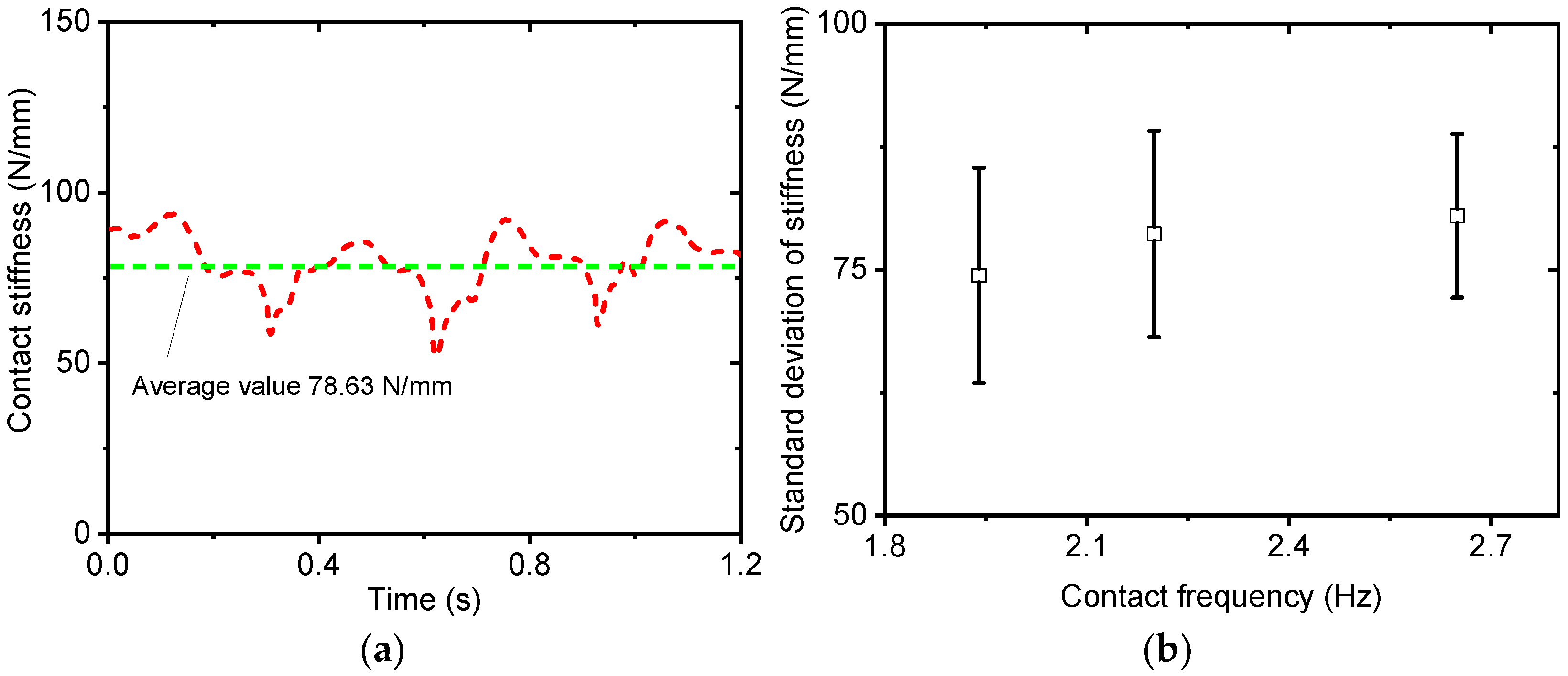
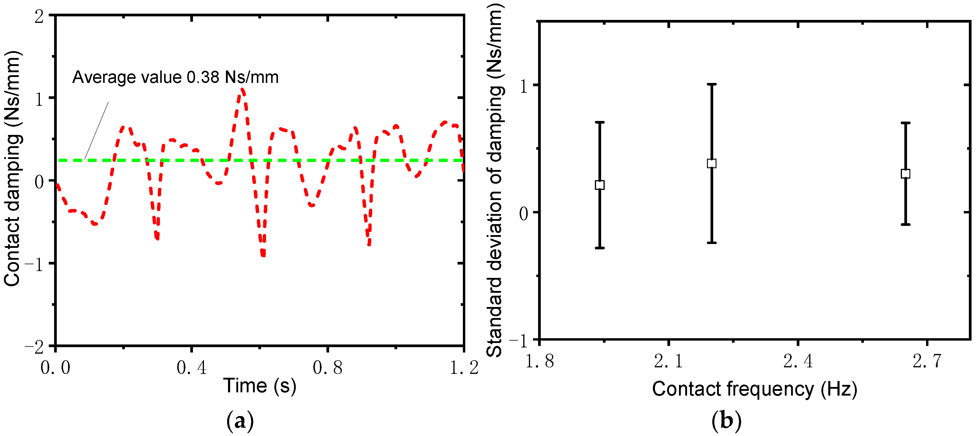
3.3. Damping Estimation

The above subsection provides a series PC method with impedance causality for preventing the velocity divergence of a HIL simulation. For the impedance configuration, vdes(k) = vact(k) is the input and the PC compensation force, Fcomp(k) and Mcomp(k) are the outputs. In an ideal case (i.e., the contact damping in Equation (9) is not considered), contact velocities always remain unchangeable during the whole HIL simulation. However, this result does not represent the practical case in which the damping dissipation exists inevitably. Therefore, to reproduce the practical contact dynamics in space, contact damping is necessary to be identified in the HIL simulation.
The position and velocity of the contact point with respect to the global coordinate system in Figure 8 are written as
p O P ( k ) = p IE ( k ) + R IE b ( k ) r O P O IE ( k ) ,
v O P ( k ) = v IE ( k ) + ω dm ( k ) × ( R IE b ( k ) r O P O IE ( k ) ) ,
where r O P O IE is the position vector of the contact point with respect to {OIE}; R IE b is the transformation matrix from frame {OIE} to frame {Obase}; ωdm is the angular velocity of the docking-mimicking mechanism.
At the time k, given the force Fs(k), the deformation and velocity at the contact point along the direction of contact force can be obtained as
Δ p s ( k ) = ( p O P ( k ) p O P ( k 1 ) ) T F s ( k ) F s ( k ) ,
Δ v s ( k ) = ( v O P ( k ) v O P ( k 1 ) ) T F s ( k ) F s ( k ) ,
Δ F s ( k ) = ( F s ( k ) F s ( k 1 ) ) F s ( k ) F s ( k ) .
Since the sampling time for the force measurement is very short, contact stiffness and contact damping can be regarded as fixed values in one sampling time. Thus, the following relationship can be obtained:
Δ F s ( k ) = k d Δ p s ( k ) + c d Δ v s ( k ) ,
where kd and cd are the equivalent contact stiffness and damping along the contact force. To effectively evaluate the identification algorithm, the facility robot always remains a fixed configuration during the contact process. Therefore, the identified values can be regarded as an overall stiffness and damping, including the facility robot and the docking-mimicking mechanism.
For the above contact process, the Sage–Husa adaptive Kalman filter (AKF) is used to predict and update the estimation values of contact parameters, which is written as
{ X ( k ) = A ( k 1 ) X ( k 1 ) + G ( k 1 ) W ( k 1 ) Z ( k ) = H ( k ) X ( k ) + V ( k ) ,
where X(k) = [kd(k), cd(k)]T is the state vector; Z(k) = ΔFs(k) is the measurement vector; W(k − 1) is the measurement noise at k − 1; V(k) is observation noise; A(k) is the state-transition matrix from k − 1 to k; G(k) is the system noise matrix; and H(k) = [Δps(k), Δvs(k)]T is the observation matrix. Since there are two state variables, both A and G are 2 × 2 identity matrices. The detailed process of solving AKF equations can be found in [30].
Accordingly, the contact damping can be identified when a groups of increments ΔFs(k), Δps(k), and Δvs(k) are given. Although the contact stiffness is simultaneously estimated, the presented control strategy does not require the contact stiffness. In Section 4, the comparison of the identified stiffness and the theoretical value is carried out only to verify the identification method.

3.4. Control Strategy

As shown in Figure 9, the whole process of the proposed passivity-based control strategy for the HIL simulation is given as follows:
(1)
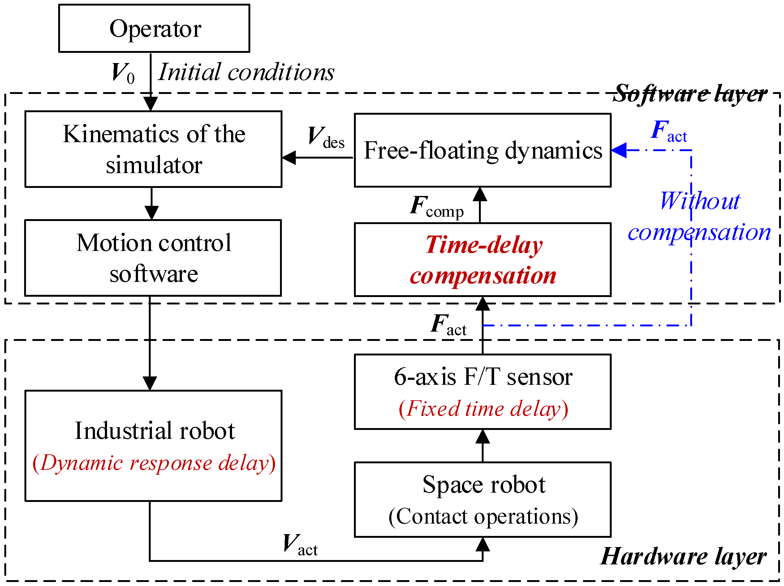
Given the initial displacements, velocities, and accelerations of two satellites, s0, v0, and a0, respectively, the robotic simulator follows the motion trajectory to realize the first collision between the docking imitation mechanisms.
(2)
The six-axis F/T sensor measures the contact force and moment, Fmea and Mmea. Then, the pure time delay τm caused by the measurement system is compensated by a low-pass filter, and the actual measuring force and moment Fs and Ms are obtained.
(3)
By substituting Fs, Ms, pOp, and vOp into Equations (16)–(22), the contact damping, cd, is identified using the AKF method.
(4)
According to the identified contact damping, the elastic contact force, Fek, is calculated. Then, by substituting Fek, Ms, v des , and ω des into the PO yields the time-varying damping matrix, and thus the PC compensation force and moment, Fα and Mα, are calculated through Equations (12) and (14). Accordingly, the compensated force and moment, Fcomp and Mcomp, are obtained using Equation (15).
(5)
Fcomp and Mcomp are substituted into the space dynamic equations, Equations (3) and (4), to calculate the new motion trajectory of the robotic simulator, including s, v, and a. By repeating steps (1)–(5), the HIL simulation can be continued until the conclusion of the experiment.

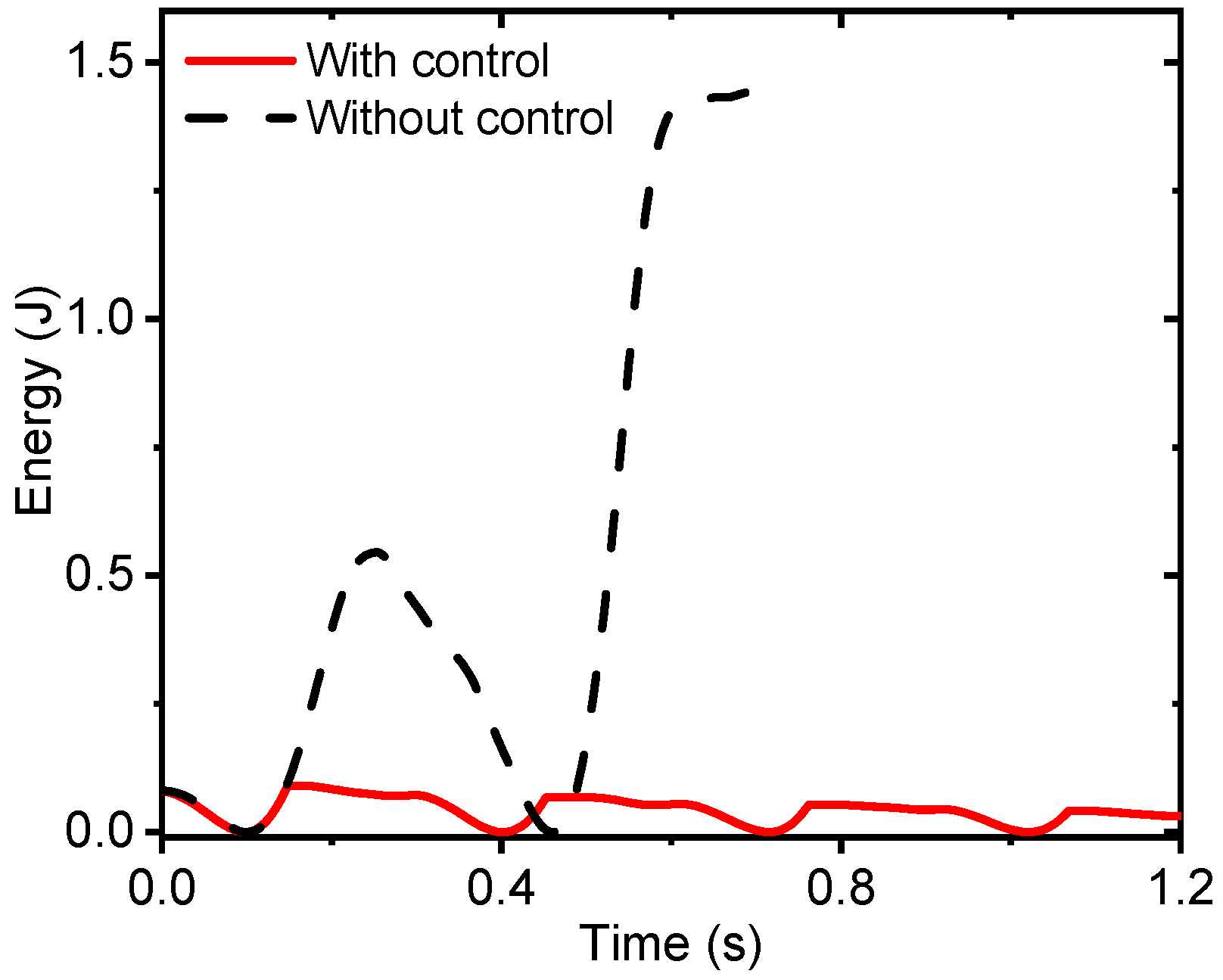
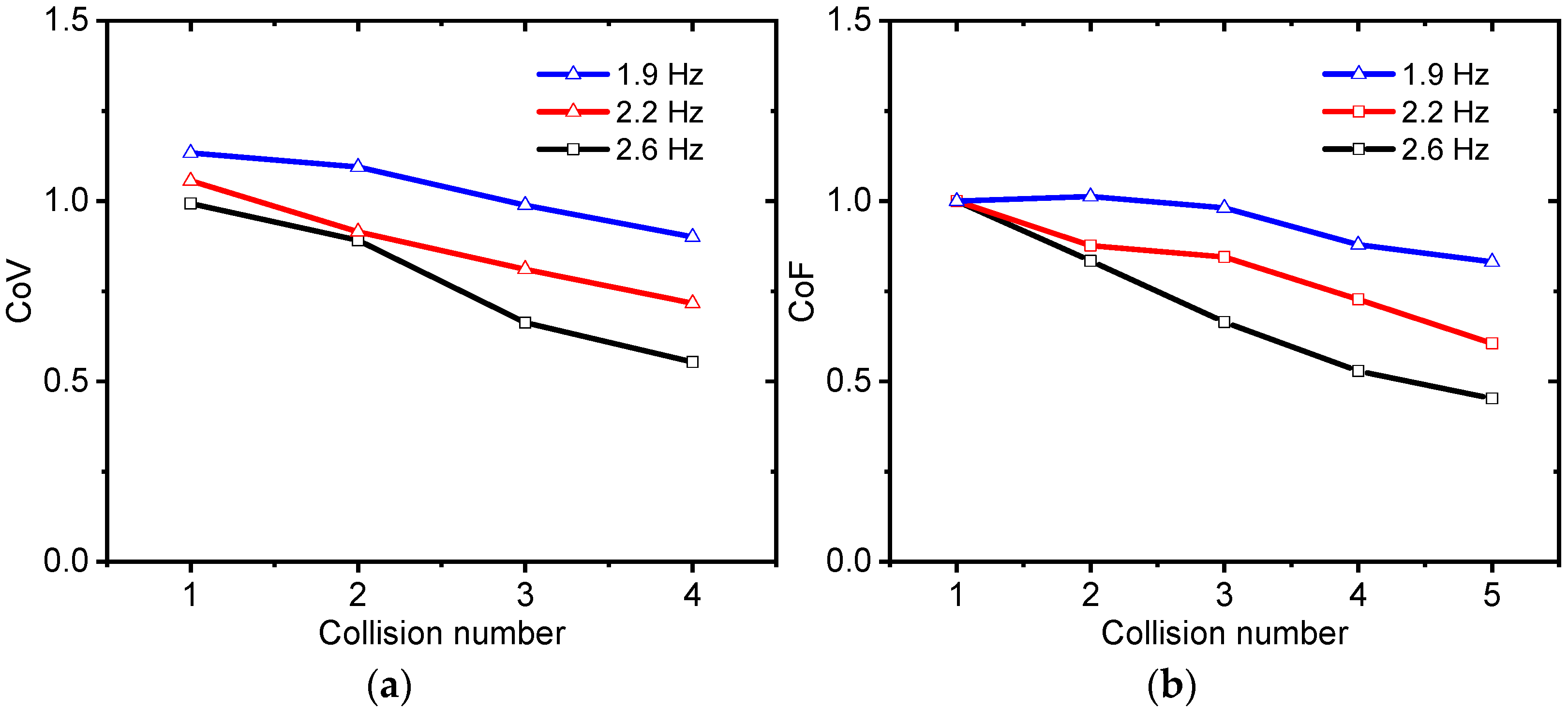
4. Experiment and Discussion

To verify the proposed control strategy, two groups of experiments are carried out on the HIL simulation system, namely collision experiments against a virtual wall, and the real contact experiments between the collision rod and the frame. On one hand, for the virtual collision, contact forces are generated through colliding against a virtual wall, which is modelled as a spring-damper system. Both the contact stiffness and damping of a virtual wall are the fixed values. Through comparing the estimated stiffness and damping with them, the contact parameter estimation method can be verified. On the other hand, for the real contact experiments, the whole control strategy can be verified. Figure 10 shows an example of one real contact process. Since the velocity remains unchangeable between the front frame and the rear frame, these data are removed in the following experimental curves and the left data are connected to show only the contact process more clearly.

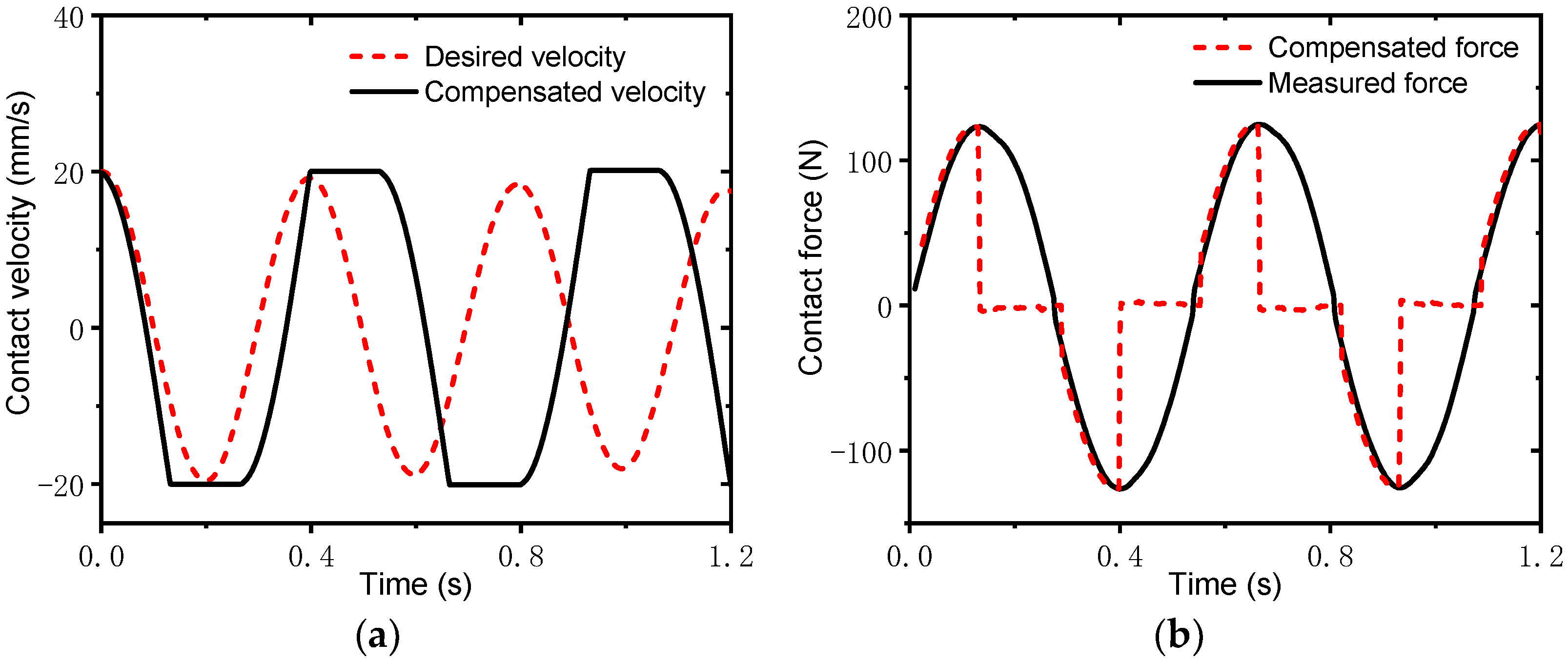
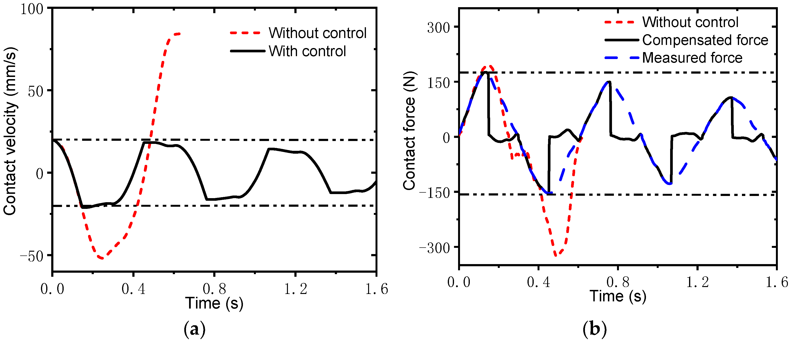
4.1. Collisions against a Virtual Wall

In this section, collision experiments against a virtual wall are carried out. The experimental parameters are given as follows. The masses of the servicing satellite and the target satellite are 300 kg and 4000 kg, respectively. The inertia parameters of the servicing satellite are Ixx = Iyy = Izz = 98 kg∙m2. The inertia parameters of the target satellite are Ixx = Iyy = Izz = 3684 kg∙m2. The initial linear and angular velocities are v = [0.02, 0, 0]T and ω = [0, 0, 0]T, respectively.
The virtual wall is a spring-damper system, which is denoted by
F s = k g · p + S t e p ( p , 0 , 0 , p max , c g ) · d p d t ,
where kg = 70 N/mm is the contact stiffness. Since contact damping is a variable with respect to the depth of penetration, a Step function is defined to describe the damping, given by
S t e p ( p , 0 , 0 , p max , c g ) = { 0 p 0 c g · ( p p max ) 2 ( 3 2 p p max ) 0 < p < p max c g p p max ,
where cg = 0.1 Ns/mm; p is the depth of penetration; pmax is the maximum penetration depth.
Figure 11 presents the estimates of contact stiffness and contact stiffness. It is found that contact stiffness and damping are both identified very well. The average of identified stiffnesses is 70.23 N/mm and the maximum of stiffness errors is less than 7%. The average damping is 0.068 Ns/mm, which is close to the given value. The errors of the identified damping are larger than the stiffness errors. Figure 12 gives contact forces and contact velocities. It can be observed that the practical contact forces (i.e., the measured contact forces) remain stable. The maximum of the contact forces after each collision almost remains unchangeable. As mentioned above, the intrinsic time delay of an industrial robot leads to energy increase and simulation divergence. However, the rebound velocities for each collision almost correspond to the desired velocities, which validates the proposed passivity-based control strategy.

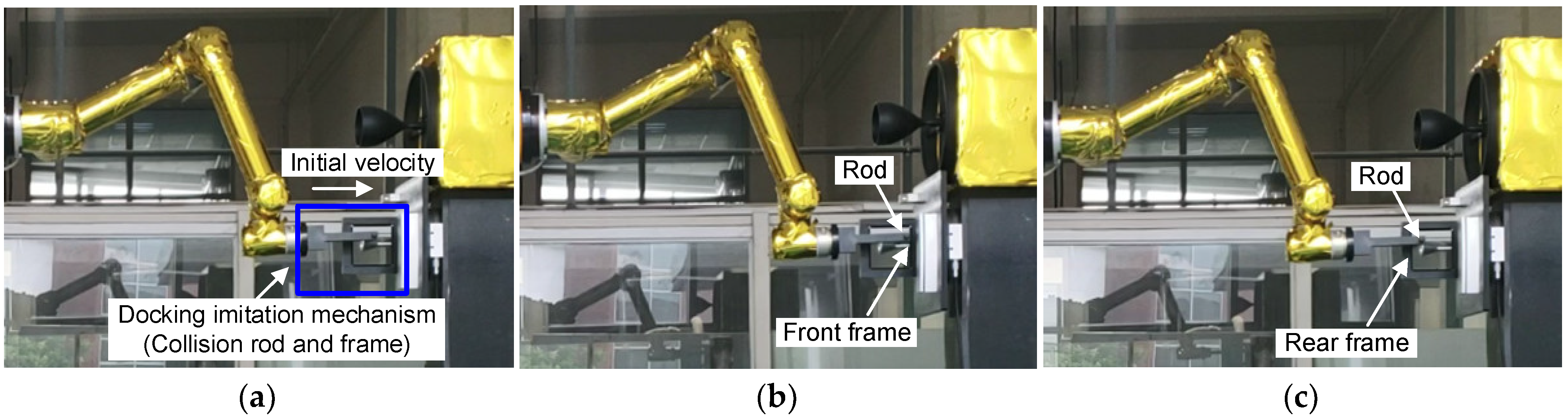
4.2. Collisions between Docking Imitation Mechanisms

As an example, the masses of the servicing satellite and the target satellite are given as 450 kg and 4000 kg, respectively. The inertia parameters of two satellites and the initial contact velocity are the same as those in collision experiments against a virtual wall. Figure 13a shows the identified contact stiffness. To describe clearly the contact process, a contact frequency can be defined using an average stiffness, as follows:
f = 1 2 π k ¯ d m e ,
where me = msmt/(ms + mt) is the relative mass; ms and mt are the masses of the service and target satellites, respectively; k ¯ d is the average contact stiffness. The average stiffness for ms = 450 kg is 78.63 N/mm; thus, the contact frequency is obtained as 2.2 Hz. To further validate the control strategy, different contact frequencies are chosen by changing the mass of the servicing satellite. Figure 13b gives the average and the standard deviation of the stiffness estimates with respect to different contact frequencies. Here, the standard deviation is denoted by
σ = 1 N i = 1 N ( k d i k ¯ d ) 2 ,
where kdi is the identified contact stiffness every time. It is found that the averages of the identified stiffnesses for three contact frequencies are very close. In addition, Figure 14 shows the identified contact damping at f = 2.2 Hz and the standard deviation of the damping estimates. It is observed that the averages of the damping estimates for different frequencies are also very close. Note that there exists obvious negative damping during the experiments. The main reason is that force noises lead to large deflections of the estimation error covariance of the AKF. In the control loop, substituting the negative damping factor into the force compensation formula yields the increase in the system energy. Accordingly, the estimated results for different contact frequencies verify the proposed method for contact parameter identification.
Figure 15 shows the contact velocities and the contact forces at f = 2.2 Hz. There is significant velocity divergence without control because of the time delay. However, the simulation divergence can be prevented by the proposed control strategy. Although there is a slight overshoot of contact velocity for the first collision, the contact velocity converges gradually after two collisions. The time delay in the HIL simulation system leads to a significant force divergence without control, as observed in Figure 15b. To avoid the damage of the imitation docking mechanisms, the experiments without control have to be stopped at the second collision. However, using the proposed passivity-based control strategy, large impact forces at the second collision are prohibited. The contact forces decrease with the decrease in the contact velocities. The contact force convergence occurs. The energy change at f = 2.2 Hz in Figure 16 also shows that the energies without control increase significantly. Using the proposed control method, the energy decreases little by little due to the damping dissipation.
To further illustrate the effect of the control strategy on the simulation divergence, a coefficient of velocity (CoV) and a coefficient of contact force (CoF) are defined. The CoV is defined as the ratio of the rebound velocity to the desired velocity (i.e., the initial velocity) [17]. During practical contact experiments, both the theoretical contact stiffness and damping are unknown. Thus, the desired contact force cannot be obtained in practical experiments. Therefore, the CoF is defined as the ratio of the maximum contact force during each collision to the maximum contact force during the first collision. Figure 17 shows the CoVs and CoFs during the experiments with respect to different contact frequencies. It is found that the convergence phenomena occur more obviously with the increase in contact frequency. Meanwhile, contact forces for different contact frequencies show similar changes to the contact velocities. Accordingly, the proposed control strategy can deal with the simulation divergence for different contact frequencies.

5. Conclusions

This study proposes a passivity-based velocity control method for HIL simulation systems with time delay. A HIL simulation system is presented using a common industrial robot and its existing problems are investigated. It is found that there is obvious velocity divergence without delay compensation, even if a very small time delay exists. After that, the control strategy is conducted for the velocity divergence, which consists of the PO, the PC, and the damping identification module. The energy flow of the HIL simulation system is analyzed and then the PO is defined. The contact damping identified in real time is introduced into the PC. Thus, the modified damping factor is capable of representing the energy dissipation due to the damping force during a real physical contact process in space. Finally, collision experiments against a virtual wall and collision experiments between docking-mimicking mechanisms are both implemented. The experimental results show that the velocity divergence due to time delay has been prevented by the proposed control strategy, and that the velocity characteristics with high fidelity are obtained.
Currently, only the velocity characteristics of the HIL simulation system are involved in the control strategy. However, the contact force characteristics cannot be handled by the proposed control method, which is determined by the passivity principle. The passivity-based control adjusts the contact velocities to conform to the energy conservation; thus, the accuracy of the contact force is inevitably sacrificed. Moreover, the pure velocity control is likely to produce large contact forces, which will damage the tested instruments. Therefore, a hybrid force/velocity control method for the HIL simulation requires further study.

Author Contributions

Conceptualization, J.H. and F.G.; methodology, M.S.; software, M.S.; investigation, J.H. and M.S.; writing—original draft preparation, J.H.; writing—review and editing, J.H.; supervision, F.G.; funding acquisition, J.H. All authors have read and agreed to the published version of the manuscript.

Funding

This research was funded by National Natural Science Foundation of China, grant no. 52175022, the State Key Laboratory of Mechanical System and Vibration, grant no. MSVZD202106, and Shanghai R&D public service platform project, grant no. 19DZ2291400.

Institutional Review Board Statement

Not applicable.

Informed Consent Statement

Not applicable.

Data Availability Statement

Data will be made available upon reasonable request by the corresponding author.

Conflicts of Interest

The authors declare no conflict of interest.

References

  1. Flores-Abad, A.; Ma, O.; Pham, K.; Ulrich, S. A review of space robotics technologies for on-orbit servicing. Prog. Aerosp. Sci. 2014, 68, 1–26. [Google Scholar] [CrossRef] [Green Version]
  2. Ma, B.; Xie, Z.; Jiang, Z.; Liu, H. Precise semi-analytical inverse kinematic solution for 7-DOF offset manipulator with arm angle optimization. Front. Mech. Eng. 2021, 16, 435–450. [Google Scholar] [CrossRef]
  3. Qi, C.; Ren, A.; Gao, F.; Zhao, X.; Wang, Q.; Sun, Q. Compensation of Velocity Divergence Caused by Dynamic Response for Hardware-in-the-Loop Docking Simulator. IEEE/ASME Trans. Mechatron. 2016, 22, 422–432. [Google Scholar] [CrossRef]
  4. Ma, O.; Wang, J. Model order reduction for impact-contact dynamics simulations of flexible manipulators. Robotica 2007, 25, 397–407. [Google Scholar] [CrossRef]
  5. Virgili-Llop, J.; Drew, J.V.; Zappulla, R.; Romano, M. Laboratory experiments of resident space object capture by a spacecraft–manipulator system. Aerosp. Sci. Technol. 2017, 71, 530–545. [Google Scholar] [CrossRef]
  6. He, J.; Zheng, H.; Gao, F.; Zhang, H. Dynamics and control of a 7-DOF hybrid manipulator for capturing a non-cooperative target in space. Mech. Mach. Theory 2019, 140, 83–103. [Google Scholar] [CrossRef]
  7. Carignan, C.; Akin, D. The reaction stabilization of on-orbit robots. IEEE Control Syst. 2000, 20, 19–33. [Google Scholar] [CrossRef]
  8. Watanabe, Y.; Nakamura, Y. Experiments of a space robot in the free-fall environment. In Proceedings of the 5th International Symposium on Artificial Intelligence, Robotics and Automation in Space, Noordwijk, The Netherlands, 1–3 June 1999. [Google Scholar]
  9. Shimoji, H.; Inoue, M.; Tsuchiya, K.; Niomiya, K.; Nakatani, I.; Kawaguchi, J. Simulation system for a space robot using six-axis servos. Adv. Robot. 1991, 6, 179–196. [Google Scholar] [CrossRef] [Green Version]
  10. Mitchell, J.D.; Cryan, S.P.; Baker, K.; Martin, T.; Goode, R.; Key, K.W.; Manning, T.; Chien, C. Integrated docking simulation and testing with the Johnson Space Center six-degree-of-freedom dynamic test system. In Proceedings of the Space Technology and Applications International Forum—STAIF 2008, Albuquerque, NM, USA, 10–14 February 2008. [Google Scholar]
  11. Takahashi, R.; Ise, H.; Konno, A.; Uchiyama, M.; Sato, D. Hybrid simulation of a dual-arm space robot colliding with a floating object. In Proceedings of the IEEE International Conference on Robotics and Automation, Pasadena, LA, USA, 19–23 May 2008. [Google Scholar]
  12. Matunaga, S.; Yoshihara, K.; Takahashi, T.; Tsurumi, S.; Ui, K. Ground experiment system for dual-manipulator-based capture of damaged satellites. In Proceedings of the IEEE/RSJ International Conference on Intelligent Robots and Systems, Takamatsu, Japan, 30 October–5 November 2000; pp. 1847–1852. [Google Scholar]
  13. Rekleitis, I.; Martin, E.; Rouleau, G.; L’Archevêque, R.; Parsa, K.; Dupuis, E. Autonomous capture of a tumbling satellite. J. Field Robot. 2007, 24, 275–296. [Google Scholar] [CrossRef]
  14. Ma, O.; Flores-Abad, A.; Boge, T. Use of industrial robots for hardware-in-the-loop simulation of satellite rendezvous and docking. Acta Astronaut. 2012, 81, 335–347. [Google Scholar] [CrossRef]
  15. Sellmaier, F.; Boge, T.; Spurmann, J.; Gully, S.; Rupp, T.; Huber, F. On-orbit servicing missions: Challenges and solutions for spacecraft operations. In Proceedings of the 11th International Conference on Space Operations, Huntsville, AL, USA, 25–30 April 2010. [Google Scholar]
  16. Gao, F.; Qi, C.; Ren, A.; Zhao, X.; Cao, R.; Sun, Q.; Wang, Q.; Hu, Y.; He, J.; Jin, Z.; et al. Hardware-in-the-loop simulation for the contact dynamic process of flying objects in space. Sci. China Technol. Sci. 2016, 59, 1167–1175. [Google Scholar] [CrossRef]
  17. Osaki, K.; Konno, A.; Uchiyama, M. Delay Time Compensation for a Hybrid Simulator. Adv. Robot. 2010, 24, 1081–1098. [Google Scholar] [CrossRef]
  18. Diolaiti, N.; Niemeyer, G.; Barbagli, F.; Salisbury, J. Stability of Haptic Rendering: Discretization, Quantization, Time Delay, and Coulomb Effects. IEEE Trans. Robot. 2006, 22, 256–268. [Google Scholar] [CrossRef]
  19. Meng, Q.; Xie, F.; Liu, X.-J. Conceptual design and kinematic analysis of a novel parallel robot for high-speed pick-and-place operations. Front. Mech. Eng. 2017, 13, 211–224. [Google Scholar] [CrossRef] [Green Version]
  20. Abiko, S.; Satake, Y.; Jiang, X.; Tsujita, T.; Uchiyama, M. Delay time compensation based on coefficient of restitution for collision hybrid motion simulator. Adv. Robot. 2014, 28, 1177–1188. [Google Scholar] [CrossRef]
  21. Arnold, V.I. Mathematical Methods of Classical Mechanics, 2nd ed.; Springer: New York, NY, USA, 1989; pp. 59–60. [Google Scholar]
  22. Colgate, J.E.; Hogan, N. Robust control of dynamically interacting systems. Int. J. Control 1988, 48, 65–88. [Google Scholar] [CrossRef]
  23. Berghuis, H.; Nijmeijer, H. A passivity approach to controller-observer design for robots. IEEE Trans. Robot. Autom. 1993, 9, 740–754. [Google Scholar] [CrossRef] [Green Version]
  24. Ajwad, S.A.; Iqbal, J.; Ullah, M.I.; Mehmood, A. A systematic review of current and emergent manipulator control approaches. Front. Mech. Eng. 2015, 10, 198–210. [Google Scholar] [CrossRef]
  25. Ryu, J.-H.; Kwon, D.-S.; Hannaford, B. Stability Guaranteed Control: Time Domain Passivity Approach. IEEE Trans. Control Syst. Technol. 2004, 12, 860–868. [Google Scholar] [CrossRef] [Green Version]
  26. Ryu, J.-H.; Kwon, D.-S.; Hannaford, B. Stable Teleoperation with Time-Domain Passivity Control. IEEE Trans. Robot. Autom. 2004, 20, 365–373. [Google Scholar] [CrossRef]
  27. Hannaford, B.; Ryu, J.H. Time domain passivity control of haptic interfaces. In Proceedings of the IEEE International Conference on Robotics and Automation, Seoul, Korea, 21–26 May 2001. [Google Scholar]
  28. Marco, D.S.; Ribin, B.; Cristian, S. A passivity-based approach for simulating satellite dynamics with robots: Discrete-time integration and time-delay compensation. IEEE Trans. Rob. 2020, 36, 189–203. [Google Scholar]
  29. Craig, J.J. Introduction to Robotics, 3rd ed.; Pearson Education: Upper Saddle River, NJ, USA, 2005; pp. 11–117. [Google Scholar]
  30. Lu, P.; Zhao, L.; Chen, Z. Improved Sage-Husa adaptive filtering and its application. J. Syst. Simul. 2007, 19, 3503–3505. [Google Scholar]
Figure 1. The HIL simulator.
Aerospace 09 00368 g001
Figure 2. Control system of the HIL simulator.
Aerospace 09 00368 g002
Figure 3. The HIL simulation principle.
Aerospace 09 00368 g003
Figure 4. Coordinate systems of the HIL simulator.
Aerospace 09 00368 g004
Figure 5. Coordinate systems and force analysis for free-floating satellites.
Aerospace 09 00368 g005
Figure 6. Passive network representing HIL simulation system. (a) Traditional control system view. (b) Network point of view.
Aerospace 09 00368 g006
Figure 7. Modelling in electrical domain with velocity conserving.
Aerospace 09 00368 g007
Figure 8. Description of contact process. (a) Position of contact point. (b) Velocity and force at contact point.
Aerospace 09 00368 g008aAerospace 09 00368 g008b
Figure 9. Control architecture.
Aerospace 09 00368 g009
Figure 10. An example of contact process. (a) Initial position. (b) Contact with front frame. (c) Contact with rear frame.
Aerospace 09 00368 g010
Figure 11. Estimates of contact stiffness and damping in virtual collisions. (a) Stiffness. (b) Damping.
Aerospace 09 00368 g011
Figure 12. Estimates of contact velocities and forces in virtual collisions. (a) Velocities. (b) Forces.
Aerospace 09 00368 g012
Figure 13. Estimates of stiffness in real collisions (f = 2.2 Hz). (a) Identified results. (b) Standard deviation.
Aerospace 09 00368 g013
Figure 14. Estimates of damping in real collisions (f = 2.2 Hz). (a) Identified results. (b) Standard deviation.
Aerospace 09 00368 g014
Figure 15. Contact velocities and forces in experiments (f =2.2 Hz). (a) Velocities. (b) Forces.
Aerospace 09 00368 g015
Figure 16. Energy in experiments (f = 2.2 Hz).
Aerospace 09 00368 g016
Figure 17. CoVs and CoFs regarding different contact frequencies. (a) CoV. (b) CoF.
Aerospace 09 00368 g017
Table 1. Specifications of the HIL simulator.
ModuleSpecificationsUnitValue
Industrial robotDoF-6
Payloadkg210
Maximum reachmm2674
Repeatabilitymm±0.3
RailDoF-1
Payloadkg3000
Lengthmm12,000
Speedmm/s1600
Repeatabilitymm±0.05
Space robotDoF-6
Payloadkg5
Maximum reachmm800
Repeatabilitymm±0.1
Publisher’s Note: MDPI stays neutral with regard to jurisdictional claims in published maps and institutional affiliations.

