A Preliminary Top-Down Parametric Design of Electromechanical Actuator Position Control

Abstract

A top-down process is proposed and virtually validated for the position control of electromechanical actuators (EMA) that use conventional cascade controllers. It aims at facilitating the early design phases of a project by providing a straightforward mean that requires simple algebraic calculations only, from the specified performance and the top-level EMA design parameters. This makes it possible to include realistic control considerations in the preliminary sizing and optimisation phase. The position, speed and current controllers are addressed in sequence. This top-down process is based on the generation and use of charts that define the optimal position gain, speed loop second-order damping factor and natural frequency with respect to the specified performance of the position loop. For each loop, the control design formally specifies the required dynamics and the digital implementation of the following inner loop. A noncausal flow chart summarises the equations used and the interdependencies between data. This potentially allows changing which ones are used as inputs. The process is virtually validated using the example of a flight control actuator. This is achieved with resort to the simulation of a realistic lumped-parameter model, which includes any significant functional and parasitic effects. The virtual tests are run following a bottom–up approach to highlight the pursuit and rejection performance. Using low-, medium- and high-excitation magnitudes, they show the robustness of the controllers against nonlinearities. Finally, the simulation results confirm the soundness of the proposed process.

1. Introduction

The last decade has seen significant progress in electromechanical technology for actuation. In the range of some kilowatts or some tens of kilonewtons, they provide attractive solutions compared with the servohydraulic (or so-called conventional) technology [1]. This evolution is particularly observed in aerospace, which is looking for greener actuation for flight controls, landing gears and engines.

For many applications, electromechanical actuators (EMAs) have already reached the highest technology readiness level, TRL9, which enables them to be put into service. However, it appears that EMAs for aerospace cannot be standardised easily, as opposed to those devoted to industrial applications. This mainly comes from the specificity of requirements and constraints that concern the geometrical integration, the reliability, the mission profiles (including four-quadrant operation with numerous and rapid changes between quadrants) and the certifiability and development assurance level (DAL). The EMA control design itself is driven by these considerations.

Although commercially off-the-shelf drives for industrial applications include efficient self-tuning features [2], each aerospace actuation project requires a specific activity for control design, which must suit the application constraints and development timing in a systems-engineering (SE) frame [3]. There are potentially many candidate types of controllers that today offer extended possibilities: for example, R-S-T digital polynomial controllers (combining parallel R, series S and feedforward T corrections), state feedback controllers with an estimator, nonlinear controllers or adaptive controllers, for example [4,5,6,7]. On their side, EMAs have numerous technology imperfections (e.g., friction and backlash) that are highly sensitive to the operating point. This generally greatly penalises the applicability, robustness and certifiability of these advanced controllers for safety-critical applications such as flight controls. This is why production EMAs involve quite conventional control strategies, which are based on fixed-gain, cascade controllers.

In the preliminary design phases of a project, the concepts and options must be benchmarked rapidly. During these early phases, emphasis is generally put on power sizing under mass, envelope, reliability and thermal constraints [8,9,10]. Although the natural dynamics of the EMA power part is sometimes addressed, control is never considered in a realistic way. This puts a high penalty on the preliminary design process for two main reasons:

• The sizing of EMAs is highly dependent on the mission profile (time history of position and force at actuator/load interface), which affects mechanical, magnetic and thermal stresses. It involves two sizing loops because the motor sizing depends on the motor design itself (rotor inertia and mean and maximal temperatures of the windings). A simple second-order representation model of the closed-loop performance is generally used to translate the mission profile from the load to the motor shaft levels. This method ignores how the controllers will solicit the EMA in practice.
• Although the power sizing ensures sufficient power capability, there is no early validation that the choices made are consistent with the specified closed-loop performance.

When the control is addressed in more detail, the well-established approach consists in using a bottom–up process [11,12]: the current loop is first addressed, and then the speed loop is considered. The position loop is rarely addressed in the literature because it is not present in many electric drives that aim to control speed (e.g., electric vehicles, fan or pump drives). For each internal loop, the bottom-up process allocates a flat-top target bandwidth that is related to the position loop specified dynamics. Unfortunately, this blind allocation deprives the control designer of a realistic and quantified view of the effective contribution of an inner loop to the stability and rapidity of its upper loops.

The research work that is reported hereafter has been driven by these considerations. It puts emphasis on the design and implementation of a top–down process that serves as a straightforward preliminary control design of a cascade position controller from top-level specifications. This work was driven by two major constraints:

• Linking formally, in a noncausal manner, the control and digital implementation parameters to the EMA dynamic specification and top-level design parameters;
• Avoiding the use of unrealistic linear control models of phenomena by verifying a posteriori the control robustness to unmodelled dynamics and nonlinearities, with resort to high-fidelity virtual tests.

Section 1 introduces the context. Section 2 details the proposed process and its implementation. The soundness of the proposal is shown in Section 3, which reports the control design validation through virtual testing. Section 4 provides important elements of discussion. The Appendix A and Appendix B merge all major resources that are used to generate the proposed preliminary control design process.

2. Top-Down Controller Design

Given the specified dynamic performance of the position loop, the proposed process outputs the proportional and integral control gains that are defined sequentially for the position, speed and current loops. Additionally, it provides the sampling frequencies for the digital implementation of the controllers, the target dynamics of the measurement chains and some values of interest for analysis purposes.

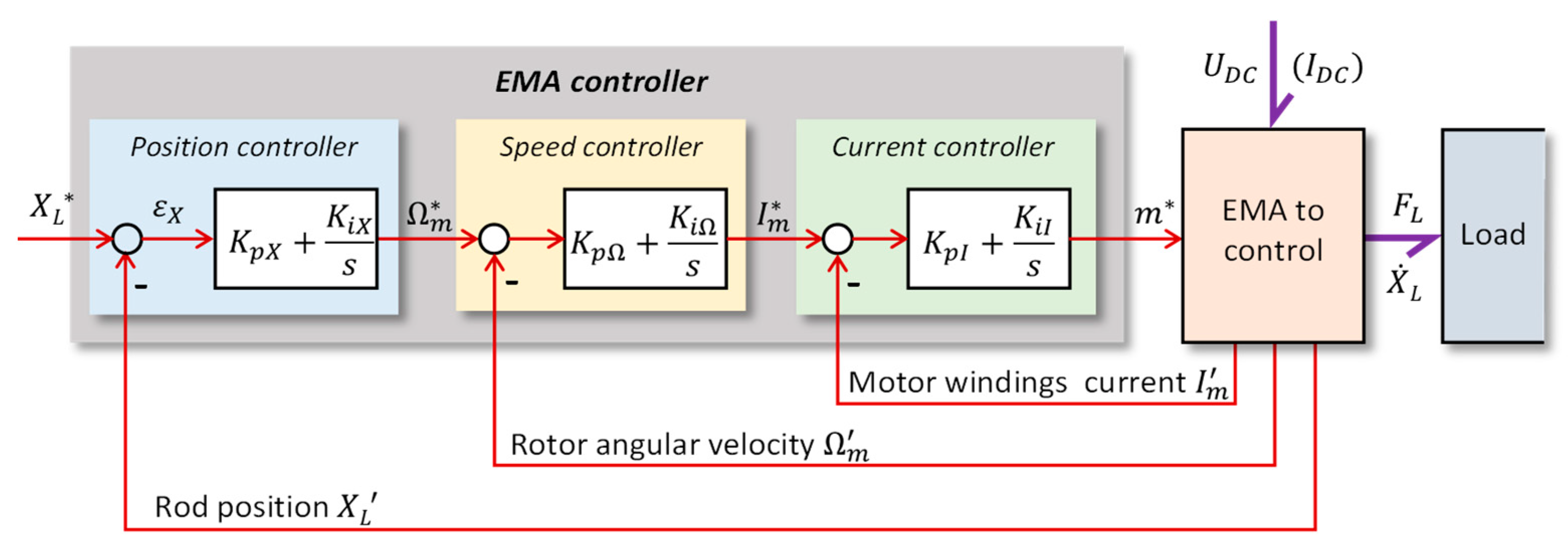
This common architecture of a cascade position controller, Figure 1, takes the benefit of the current and speed measurements that are needed to implement the brushless motor control so as to feed the controller back with measured state variables.

The current controller computes the duty cycle setpoints for the motor power drive. Current sensors and their conditioning provide the required feedback signals. The speed controller determines the current setpoints according to the power-operating domain of the motor. The speed feedback signal is commonly acquired from a resolver sensor and its resolver-to-digital converter (RDC), which measures the relative motion between the motor rotor and the stator. This chain also provides the position and speed signals for the field-oriented control (FOC) and back electromotive force (BEMF) compensation. The position controller determines the motor speed setpoint. The position feedback signal is commonly provided by a linear variometer differential transformer (LVDT), which measures the relative position between the EMA rod and the housing. In addition to the three loops, a force loop is sometimes required to meet the specific requirements related to the force limitation or rejection of dynamic loads [13].

2.1. Step 1: Design of the Position Controller and Specification of the Speed Loop Dynamics

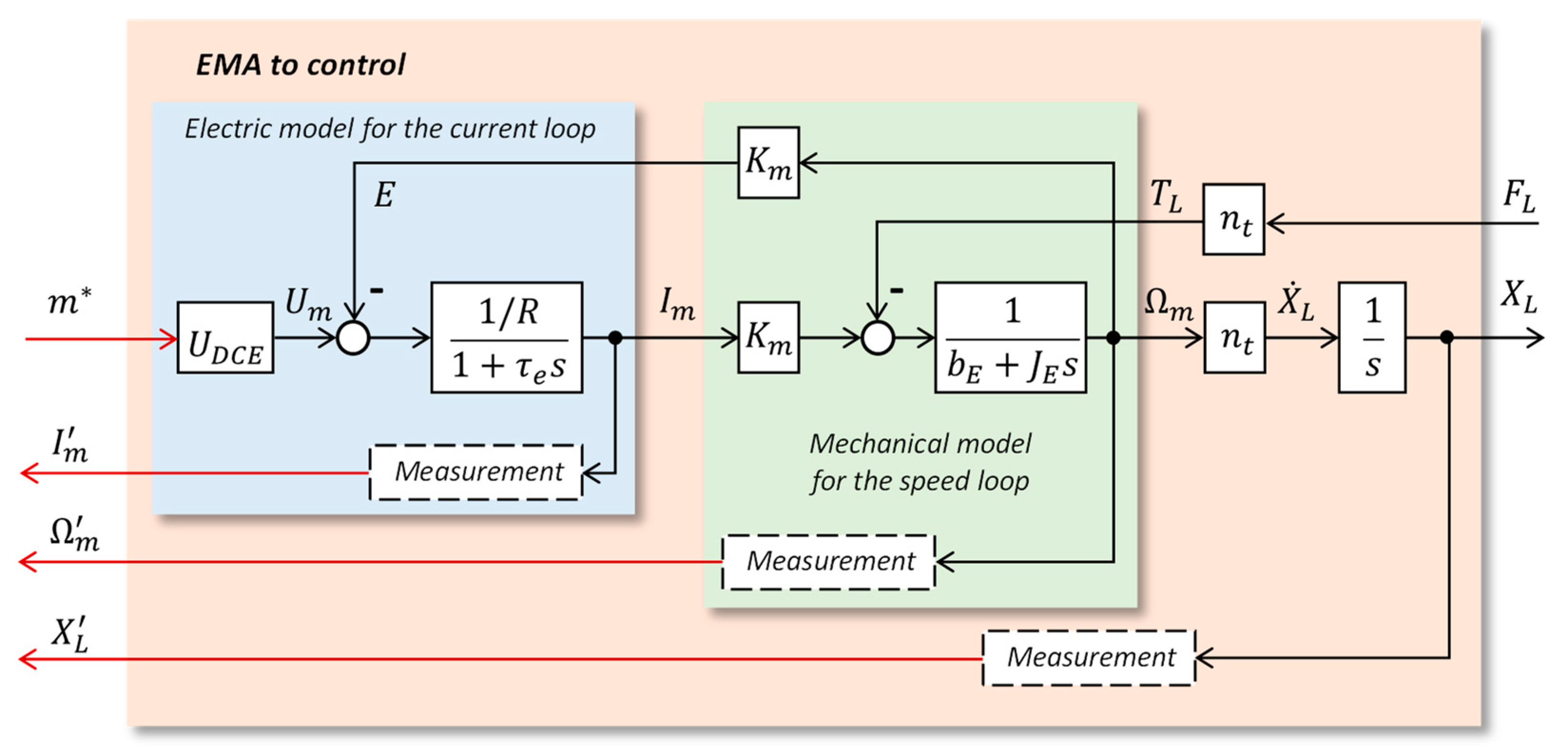
The power architecture of an aerospace EMA typically involves a three-phase inverter, which is supplied by the DC-link and drives a brushless motor of the permanent magnet synchronous machine (PMSM) type. The motor shaft power is transmitted to the driven load through a mechanical reducer (a nut-screw system in the most common direct-drive, linear EMA design). In the following, the PMSM is considered as its DC motor equivalent and the inverter is assumed to be perfect. Figure 2 displays the linear control model of the EMA that is used in the proposed process.

The first step of the process deals with the position loop. It uses as inputs the dynamic requirements of the position control, either in the frequency domain ($f_3$ frequency for −3 dB magnitude or $f_{45}$ for 45° phase lag) or in the time domain (settling time $t_{sX}$), the design margin parameter $DM$ and the transmission ratio $n_t$ of the EMA. As a result, it provides the proportional gain $K_{pX}$ of the position controller and specifies the speed loop dynamics for the second step and the minimal sampling frequency of the position controller. It also outputs additional performance indicators, in particular the angular frequency for phase margin ${\omega }_{PMX}$, which is used to specify the sampling frequency of the position controller.

According to the author’s experience, using an integral action in the position controller is not welcome for several reasons. First, the rejection of disturbances is quite low because the I gain is hardly limited by stability considerations. Second, many nonlinear effects (e.g., friction, compliance, backlash, measurement noise, quantisation) combine to produce a low-frequency limit cycle in the presence of the I action. The magnitude of the limit cycle is linked to the minimal position step that can be produced at the rod output. Therefore, it is not affected by any change in the I gain, which only acts on the frequency of this limit cycle. This explains why it is preferred to keep the position controller purely proportional, as seen in Equation (1), however with output limitation.

$${\mathsf{\Omega }}_m^{ *}=K_{pX}\left(X_L^{*}-X_L\right)$$

(1)

In the absence of friction or backlash (or compliance), the EMA internal mechanical transmission between the motor shaft and the EMA rod links the rotor and rod mechanical power variables by:

$$\{\begin{array}{c}s{X}_L=n_t{\mathsf{\Omega }}_m\\ T_L=n_t{F}_L\end{array}$$

(2)

and:

$$n_t=l/2\pi N$$

(3)

with $l$ as the nut-screw lead and $N$ as the reduction ratio of the intermediate gear.

2.1.1. Performance of the Position Loop with I-P Speed Controller

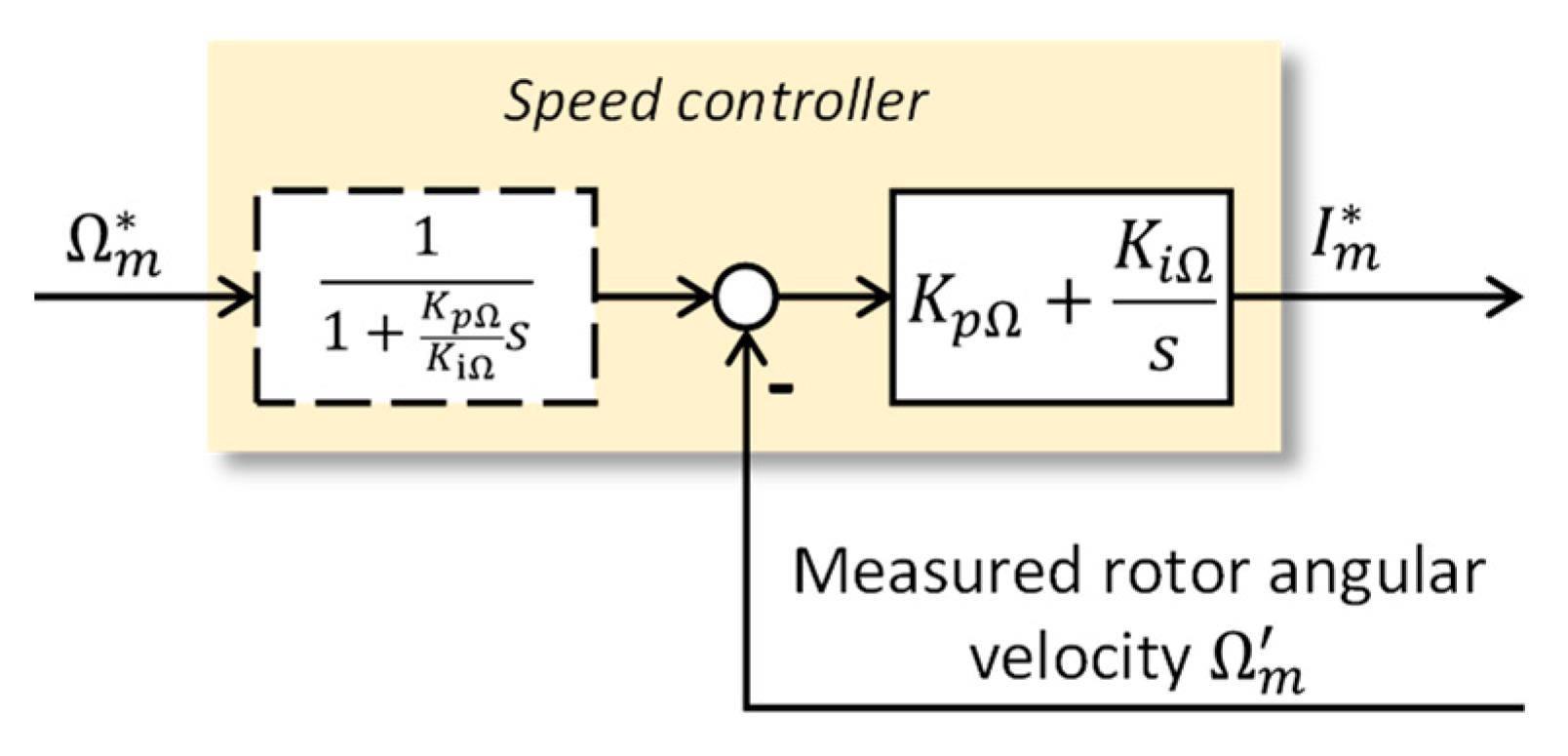
As given in

Table A2. Speed loop model and analysis in continuous-time domain.

Constitutive Equations
Perfect current control	$I_m\approx$$I_m^{*}$	Variables: $I_m$ motor actual current, $I_m^{*}$ current setpoint
PI speed controller	$I_m^{*}=\left(K_{p\mathsf{\Omega }}+K_{i\mathsf{\Omega }}/s\right)\left({\mathsf{\Omega }}_m^{*}-{\mathsf{\Omega }}_{m }^{\prime }\right)$	Parameters: $K_{p\mathsf{\Omega }}$ speed loop proportional gain, $K_{i\mathsf{\Omega }}$ speed loop integral gain Variables: $s$ Laplace variable, ${\mathsf{\Omega }}_m^{*}$ rotor speed setpoint, ${\mathsf{\Omega }}_m^{\prime }$ measured rotor speed (equals real value ${\mathsf{\Omega }}_m$ if measurement perfect)
Dynamics of the moving parts reflected at the rotor level	$J_{E}s{\mathsf{\Omega }}_m=K_m{I}_m-b_E{\mathsf{\Omega }}_m-T_L$	Parameters: $J_E$ equivalent inertia reflected at the rotor, $b_E$ equivalent viscous friction reflected at the rotor,$K_m$ motor torque constant Variables: $T_L$ EMA equivalent load reflected at the motor rotor
Speed Open-Loop Transfer
${\mathsf{\Omega }}_m=\frac{K_m\left(K_{p\mathsf{\Omega }}+K_{i\mathsf{\Omega }}/s\right)\left({\mathsf{\Omega }}_m^{*}-{\mathsf{\Omega }}_m\right)-T_L}{J_{E}s+b_E}$		Mechanical time constant ${\tau }_m=J_E/b_E$
Speed Closed-Loop Transfer
${\mathsf{\Omega }}_m=\frac{\left(1+{\tau }_{\mathsf{\Omega }}s\right){\mathsf{\Omega }}_m^{*}-\frac{1}{K_m{K}_{i\mathsf{\Omega }}}s{T}_L}{1+({\tau }_{\mathsf{\Omega }}+\frac{b_E}{K_m{K}_{i\mathsf{\Omega }}})s+\frac{J_E}{K_m{K}_{i\mathsf{\Omega }}}{s}^2}=\frac{\left(1+{\tau }_{\mathsf{\Omega }}s\right){\mathsf{\Omega }}_m^{*}-\frac{1}{K_m{K}_{i\mathsf{\Omega }}}s{T}_L}{1+\frac{2{\xi }_{\mathsf{\Omega }}}{{\omega }_{n\mathsf{\Omega }}}s+\frac{1}{{\omega }_{n\mathsf{\Omega }}^2}{s}^2}$
Static pursuit gain: ${\mathsf{\Omega }}_m/{\mathsf{\Omega }}_m^{*}$ = 1		Tracking rejection gain: ${\mathsf{\Omega }}_m/s{T}_L=1/K_m{K}_{i\mathsf{\Omega }}$
Speed controller time constant: ${\tau }_{\mathsf{\Omega }}=K_{p\mathsf{\Omega }}/K_{i\mathsf{\Omega }}$		$({\tau }_{\mathsf{\Omega }}=2{\xi }_{\mathsf{\Omega }}/{\omega }_{n\mathsf{\Omega }}$$\mathrm{if}{b}_E$ is neglected)
Denominator natural frequency: ${\omega }_{n\mathsf{\Omega }}=\sqrt{K_m{K}_{i\mathsf{\Omega }}/J_E}$		Denominator damping factor: ${\xi }_{\mathsf{\Omega }}=\frac{K_m{K}_{p\mathsf{\Omega }}+b_E}{2\sqrt{K_m{K}_{i\mathsf{\Omega }}{J}_E}}$
Controller gains for target second order: $K_{i\mathsf{\Omega }}=J_E{\omega }_{n\mathsf{\Omega }}^2/K_m$$,K_{p\mathsf{\Omega }}=\left(2J_E{\xi }_{\mathsf{\Omega }}{\omega }_{n\mathsf{\Omega }}-b_E\right)/K_m$

, the speed loop behaves as a second-order system versus the speed demand and the rate of external load. When a first-order, low-pass filter of time constant ${\tau }_{\mathsf{\Omega }}=K_{p\mathsf{\Omega }}/K_{i\mathsf{\Omega }}$ is applied to the speed demand, the controller becomes of the I-P type, and the speed loop transfer is given by:

$${\mathsf{\Omega }}_m=\frac{{\mathsf{\Omega }}_m^{*}-\frac{1}{K_m{K}_{i\mathsf{\Omega }}}s{T}_L}{1+\frac{2{\xi }_{\mathsf{\Omega }}}{{\omega }_{n\mathsf{\Omega }}}s+\frac{1}{{\omega }_{n\mathsf{\Omega }}^2}{s}^2}$$

(4)

The pole of the feedforward filter compensates the zero introduced by the speed P-I controller in the pursuit transfer function, as shown in Figure 3.

One can implement the speed controller in the I-P form because this makes the open-loop position transfer simpler. This therefore enables the closed-loop position transfer to be expressed formally in a canonical form. In this case, the open-loop position transfer for the pure proportional control of gain $K_{pX}$ and perfect position measurement ($X_L^{\prime }=X_L$) becomes, in the nonsaturated domain:

$$X_L=\frac{K_{lX}\left(X_L^{*}-X_L\right)-K_{XF}s{F}_L}{s\left[1+\frac{2{\xi }_{\mathsf{\Omega }}}{{\omega }_{n\mathsf{\Omega }}}s+\frac{1}{{\omega }_{n\mathsf{\Omega }}^2}{s}^2\right]}$$

(5)

where $F_L$ is the external load applied at the EMA rod.

The position loop gain $K_{lX}$ is linked to the position proportional gain $K_{pX}$ and the EMA transmission factor by:

$$K_{lX}=K_{pX}{n}_t$$

(6)

while the dynamic compliance of the position control is given by:

$$K_{XF}=\frac{n_t}{K_m{K}_{i\mathsf{\Omega }}{K}_{pX}}$$

(7)

which becomes:

$$K_{XF}=\frac{n_t}{K_{pX}{J}_E{\omega }_{n\mathsf{\Omega }}^2}$$

(8)

It is only linked to the motor torque constant, the EMA transmission factor and the integral control gain of the speed loop. Therefore, the $K_{pX}$ proportional position control gain depends only on the speed loop target dynamics ${\omega }_{n\mathsf{\Omega }}$ given the EMA-specified dynamics and design parameters ($K_m$, $J_E$, $n_t$).

The open-loop transfer function for position pursuit, Equation (5), combines a pure gain ($K_{lX})$ with integral and second-order dynamics (${\xi }_{\mathsf{\Omega }}$, ${\omega }_{n\mathsf{\Omega }}$). It is therefore welcome to link the closed-loop performance to these parameters in a dimensionless manner by introducing the dimensionless angular frequency $\overline{\omega }=\omega /{\omega }_{n\mathsf{\Omega }}$, which gives:

$$X_L/\left(X_L^{*}-X_L\right)=X_L/{\mathsf{\epsilon }}_X=\frac{{\overline{K}}_{lX}}{s\left(1+2{\xi }_{\mathsf{\Omega }}\overline{\omega }s+{\overline{\omega }}^2{s}^2\right)}$$

(9)

where ${\overline{K}}_{lX }=K_{lX}/{\omega }_{n\mathsf{\Omega }}$ is the dimensionless loop gain of the position loop.

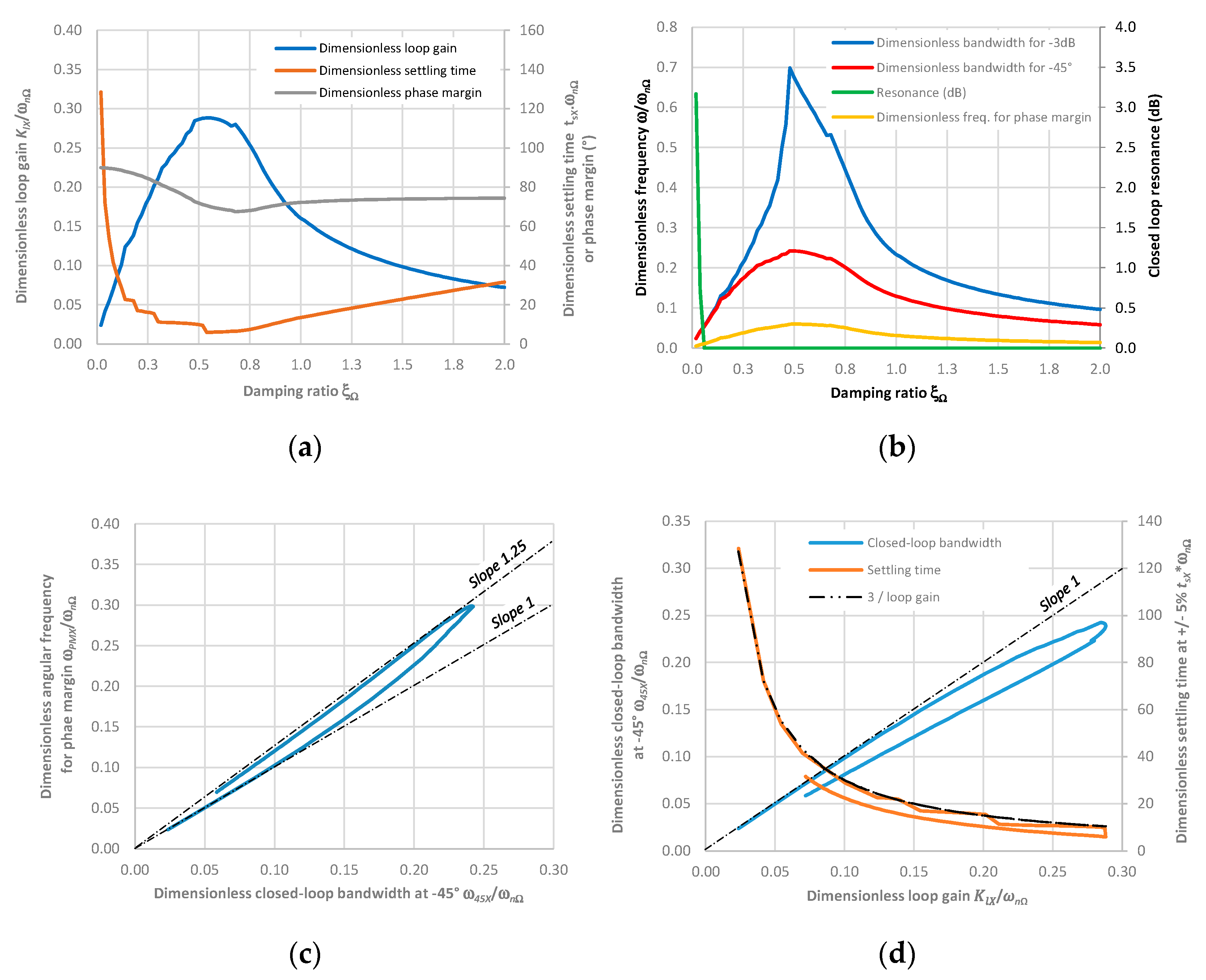
The key enabler of the proposed process is the chart that is generated once numerically. It calculates, e.g., using a control toolbox, the position closed-loop performance indicators as a function of the two parameters ${\overline{K}}_{lX}$ and ${\xi }_{\mathsf{\Omega }}$, which maximises a given constrained objective. Figure 4 displays the chart obtained to secure the fastest closed-loop response to a step position demand (minimal settling time) without overshoot. The data are generated with 1% accuracy. Particular attention is paid to the −45° phase lag requirement because it is a major one regarding the stability of the upper aircraft flight control loops.

Figure 4a displays the links among the dimensionless loop gain ${\overline{K}}_{lX}$, the phase margin and the dimensionless settling time ${\overline{t}}_s=t_{sX}.{\omega }_{n\mathsf{\Omega }}$ for a given value of the damping factor ${\xi }_{\mathsf{\Omega }}$. The best compromise between stability and rapidity is found for ${\xi }_{\mathsf{\Omega }}$ = 0.54. Figure 4b summarises the closed-loop performance indicators expressed in the frequency domain. All the values are dimensionless, with reference to ${\omega }_{n\mathsf{\Omega }}$. Again, the best bandwidth is obtained when ${\xi }_{\mathsf{\Omega }}$ is close to 0.5. Figure 4c shows that the frequency for the phase margin varies in the range of 1 to 1.25 times the closed-loop bandwidth, while the phase margin is always greater than 65° (Figure 4a). On its side, Figure 4d confirms that for low values of the loop gain, the closed-loop system is equivalent to a first-order system of time constant $1/{\overline{K}}_{lX }$. However, when the loop gain increases, the stability is affected by the closed-loop imaginary poles. The greatest dimensionless bandwidth at −45° phase is 0.287. It is obtained for ${\overline{K}}_{lX }$= 0.58, while the shortest dimensionless settling time of 5.89 is achieved for ${\overline{K}}_{lx }$= 0.54. Although ${\xi }_{\mathsf{\Omega }}$ = 0.54 minimises the settling time, such a damping generates 13% overshoot for the speed loop. Setting ${\xi }_{\mathsf{\Omega }}$ = 1 removes this overshoot. It is therefore welcome in the presence of backlash, and it still provides a good compromise for position loop stability and rapidity. However, it requires much faster speed (and current) loop dynamics than the first choices for a given dynamics of the position loop.

In the implemented approach, the control design parameter is ${\xi }_{\mathsf{\Omega }}$. The data plotted in Figure 4a or Figure 4b are first used to determine ${\omega }_{n\mathsf{\Omega }}$ and then $K_{lX}$ given the specified dynamics of the position control. This enables the $K_{pX}$ P gain of the position controller to be calculated using Equation (6) from the EMA transmission factor $n_t$.

2.1.2. Performance of the Position Loop with P-I Speed Controller

When the low-pass filter of Figure 3 is not implemented, a zero remains in the pursuit transfer function ${\mathsf{\Omega }}_m/{\mathsf{\Omega }}_m^{*}$. This P-I implementation of the speed controller also has its merits. As it does not introduce any lowpass filtering of the speed setpoint that is generated by the position controller, it decreases the tracking error. The presence of the zero that remains in the pursuit transfer function of the closed-loop position, however, tends to introduce overshoot in the position step response. Nonetheless, it does not affect the $K_{XF}$ parameter, which quantifies the load position sensitivity to the rate of external load.

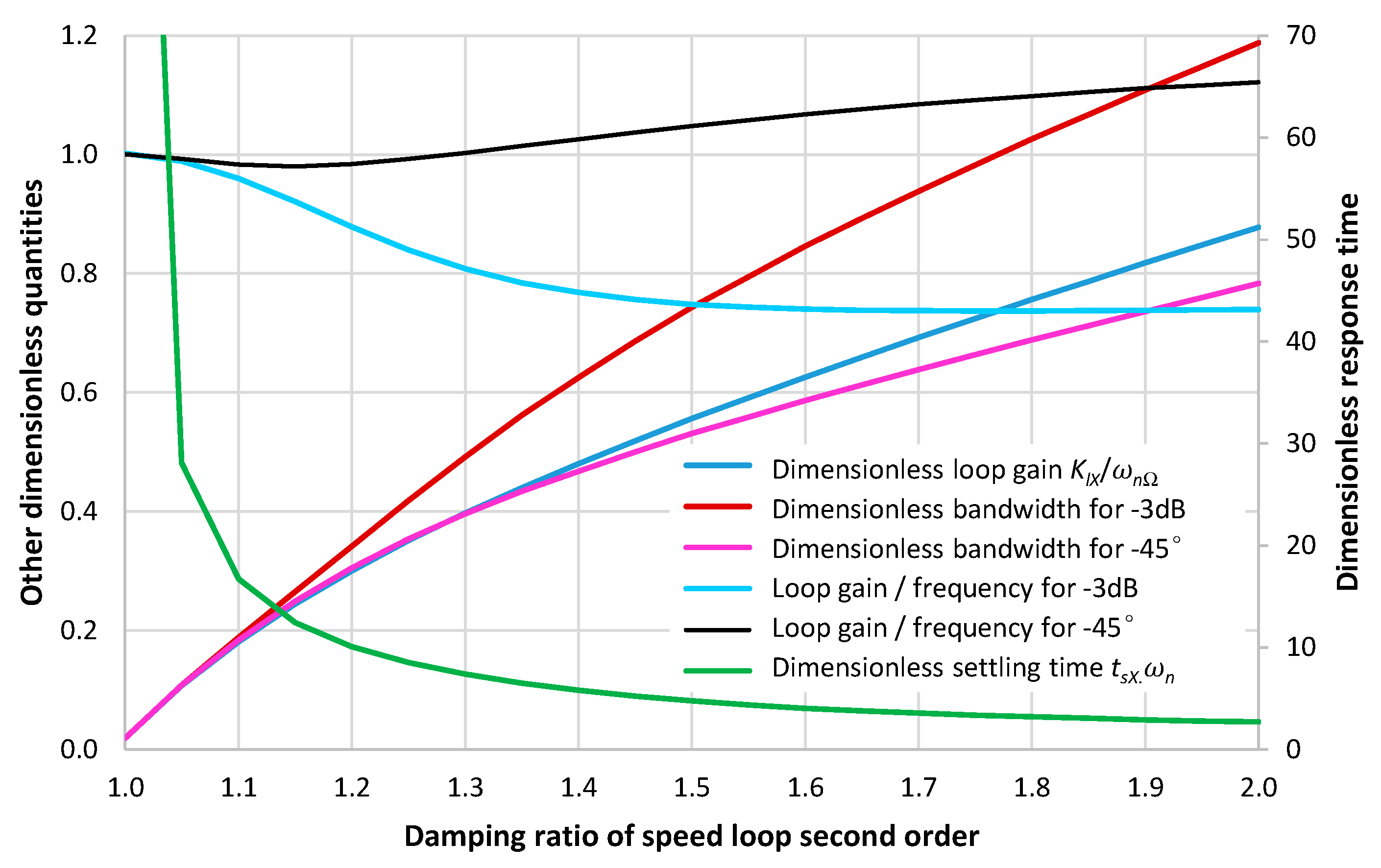
In this case, the performance chart is generated to obtain the smallest response time of the position loop, ensuring that all closed-loop poles are stable and purely real. This helps to avoid back and forth motion in the presence of backlash and limits the overshoot generated by the zero of the speed loop. The main data of this chart are presented graphically in Figure 5.

It can be remarked that the constraint imposed on the closed-loop poles cannot be met when the damping ratio ${\xi }_{\mathsf{\Omega }}$ is lower than the unity. For values greater than 1.3, this constraint significantly impacts the speed loop natural frequency compared with the I-P implementation under the null overshoot constraint. For instance, when ${\xi }_{\mathsf{\Omega }}$ = 1.3:

• The speed loop natural frequency is ${\omega }_{n\mathsf{\Omega }}$= ${\omega }_3$/0.492 = ${\omega }_{45}$/0.396 in the present case (Figure 5), while it was ${\omega }_{n\mathsf{\Omega }}$ = ${\omega }_3$/0.1601 = ${\omega }_{45}$/0.0937 formerly (Figure 4), so the present case is much less demanding in terms of speed loop (and consequently current loop) dynamics; and
• The loop gain becomes $K_{lX}={\omega }_3$/0.808 = ${\omega }_{45}$/1.002 (Figure 5), while it was $K_{lX}={\omega }_3$/0.723 = ${\omega }_{45}$/1.236 formerly (Figure 4), so the present case is disadvantageous concerning the rejection of disturbances, as shown by Equation (8).

2.1.3. Digital Implementation of the Position Controller

In this paper, the controllers are set in the continuous-time domain, using transfer functions as control models. Although this choice puts aside any advanced controller that does not exist in the continuous-time domain, it keeps a direct link with the physics through canonical parameters (time constants, damping factors and natural frequencies). Once designed, the controller is discretised for digital implementation. The phase lag introduced by filtering, sampling and computation is actively managed to specify the sampling frequencies.

When seen from the continuous-time domain, the zero-order sampling and hold function performed at the sampling frequency $f_s$ in the digital implementation of the controller is equivalent to a pure delay of ${\Delta }_s=1/2f_s$. At frequency $f$, it introduces a phase of $\phi (°)=-180 f/f_s$. In a closed-loop system, this delay is, with rare exceptions, detrimental to the closed-loop stability. This is why it is important to select the sampling frequency consistently with the target dynamics of the considered closed-loop system. There are a few practical known recommendations to make this decision [14]:

• There must be at least 7 to 15 samples in the rise time of the system response to a step input; or
• The sampling frequency must be at least 15 to 25 times the closed-loop bandwidth.

However, these general rules are not directly driven by the stability of the loop under consideration. This is why the author prefers the following more direct approach that can be expressed as follows. In total, the digital control introduces at the frequency $f$ a parasitic phase lag (phase lag stands for the opposite value of phase) ${\phi }_{d(°)}$. It comes from the sampling delay plus the phase lag of the antialiasing filter and the ${\Delta }_c$ time spent for conversions and processing. If it is assumed that the antialiasing filtering is achieved with a Butterworth second-order low-pass filter of cut-off frequency of $f_s/2$, then the phase lag is given by:

$${\phi }_{d(°)}=\frac{180}{\pi }\left[\pi /n_s+atan\left\{\frac{2.8/n_s}{1-{\left(2/n_s\right)}^2}\right\}+2\pi f_s{\Delta }_c/n_s\right]$$

(10)

where:

$$n_s=f_s/f$$

(11)

For outer loops having a low bandwidth, the delay ${\Delta }_c$ is generally negligible in comparison with other contributors. Depending on the implementation of the digital control, it may, however, be significant for the most inner (e.g., current) loops. If ${\Delta }_c$ is neglected, ${\phi }_{d(°)}$ already reaches 80.5° when $n_s$ drops to 4.35. Above this value, the phase lag of the antialiasing filter varies almost linearly versus frequency, and ${\phi }_{d(°)}$ can be approximated by:

$${\phi }_{d(°)}\cong 180 \left(1+2.8/\pi \right)/n_s\cong 340.4/ n_s$$

(12)

with less than 2.9% error of underestimation (a 360 factor, instead of 340.4, corresponds to the phase lag produced by a full sampling period delay). Antialiasing contributes to almost half the total phase lag, while the magnitude effect of the low-pass filter remains below ±0.003 dB. Of course, the ${\phi }_{d(°)}$, as shown in Equation (12), can be adapted to the current context, e.g., for the antialiasing filter or if the processing time becomes the major source of phase lag. If necessary, Equation (12) can be modified to include the phase lag introduced by the sensor and measurement chain.

These results provide a straightforward means to quantify (or specify) the reduction of the open-loop phase margin given the digital implementation of a controller that has been designed in the continuous time domain. For example, if this contribution (including the antialiasing filter) must not exceed 10° parasitic phase lag, Equation (12) indicates that the sampling frequency must be at least 34 times the frequency at which the phase margin is determined. This is a really huge value.

If the dynamics of the position measurement can be neglected, the minimal sampling frequency of the position controller can be specified using Equation (12). This option has been anticipated when building the performance charts, Figure 4 and Figure 5, which explicitly provide the angular frequency ${\omega }_{PMX}=2\pi f_{PMX}$, at which the phase margin of the position control is determined when parasitic phase lags are not considered.

Using, e.g., Equation (12), the sampling frequency $f_{sX}$ of the position controller must satisfy the constraint:

$$f_{sX}\ge 340.4 f_{PMX}/{\phi }_{dX(°)}$$

(13)

where ${\phi }_{dX(°)}$ is the allocated parasitic phase lag introduced by the digital implementation of the position controller.

Notes

• The phase lag introduced by the position measurement is not considered. Although it is generally negligible, this assumption must be verified (when the measurement chain is known), ensured by relevant specification (when the measurement chain is to be defined) or removed by adding the position measurement dynamics in Equation (13).
• For LVDTs position sensors, the demodulation filter is welcome to avoid any frequency aliasing.

2.2. Step 2: Design of the Speed Controller and Specification of the Current Loop Dynamics

2.2.1. Viscous Friction vs. Real Friction

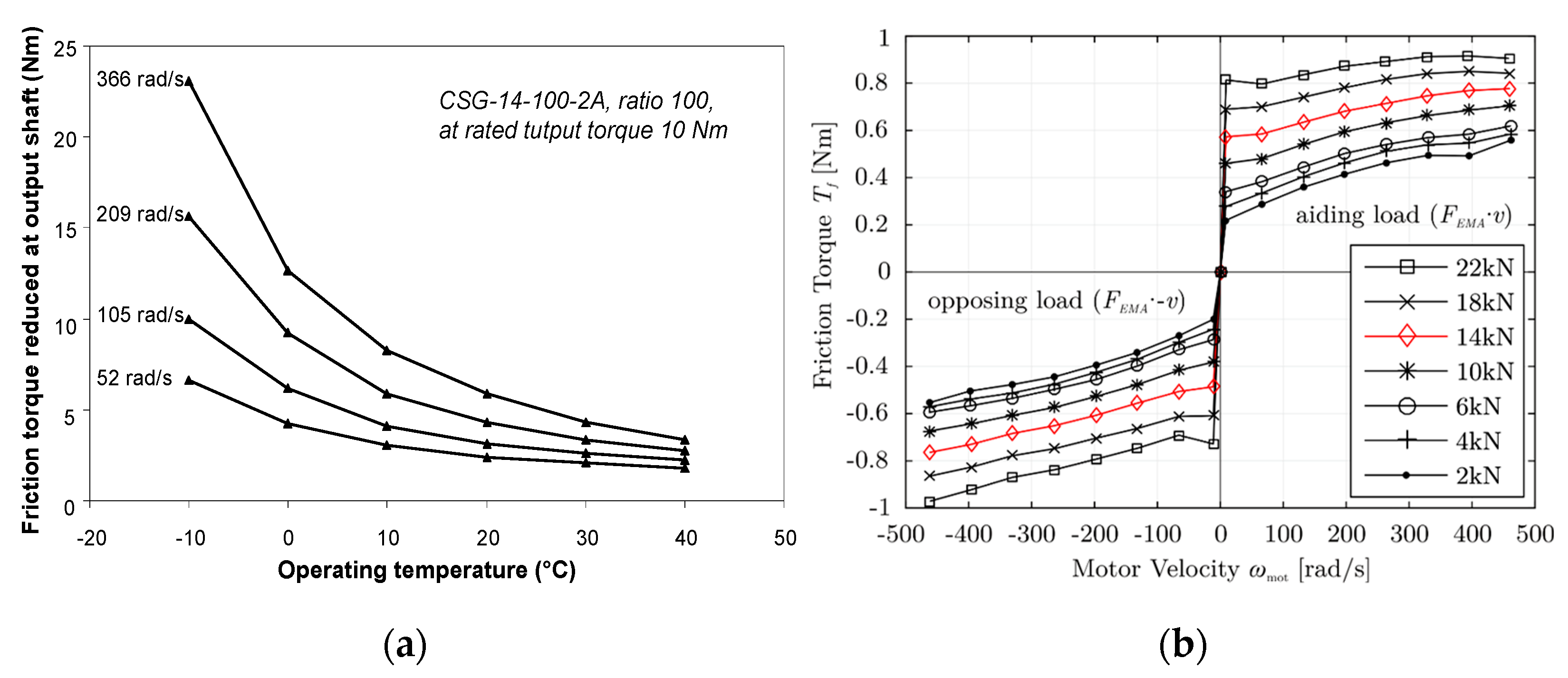
A pure viscous friction coefficient of coefficient $b_E$ is most of the time considered in the accounts dealing with setting the speed controllers of electric drives [15,16]. However, real friction is far different from pure viscous friction (where the friction force is proportional to the velocity). This is particularly true for motion control when the actuator drives a variable load at variable speed with frequent speed reversals. In this case, the friction force mainly depends on load, temperature, and, in a much lesser amount, relative speed [17]. This is clearly illustrated by the examples given in Figure 6.

This figure clearly shows that a pure viscous friction model totally fails to reproduce real friction. For linear control design, it is therefore preferred to consider friction as an unmodelled effect. This requires the controller to be robust enough against it. In this work, this robustness is assessed a posteriori, either by simulation (when validated models are available), from partial real tests or through former capitalised experience. This approach is not only applied to friction but also to backlash and compliance, whether they concern the EMA itself or the kinematics linking the EMA to the driven load. It works particularly well in the field of aerospace, e.g., for flight controls or landing gears actuation. Indeed, for such applications, the natural dynamics generated by the combination of moving bodies’ inertance and the backlash/compliance of the mechanical transmissions is far greater than the specified bandwidth of the actuator position control.

2.2.2. Setting the Speed Loop Controller

The first step of the proposed process has specified the second-order dynamics of the speed loop: the undamped natural frequency ${\omega }_{n\mathsf{\Omega }}$ and the damping factor ${\xi }_{\mathsf{\Omega }}$. These target values are used as inputs in Table A2 to obtain the proportional ($K_{p\mathsf{\Omega }}$) and integral ($K_{i\mathsf{\Omega }}$) gains of the speed controller from the total equivalent reflected inertia at the motor rotor $J_E$ and the EMA motor electromagnetic constant $K_m$:

$$K_{i\mathsf{\Omega }}=J_E{\omega }_{n\mathsf{\Omega }}^2/K_m$$

(14)

$$K_{p\mathsf{\Omega }}=2J_E{\xi }_{\mathsf{\Omega }}{\omega }_{n\mathsf{\Omega }}/K_m$$

(15)

These settings are directly linked to the specified position loop dynamics. It is interesting to remark that the time constant of the P-I speed controller,

$${\tau }_{\mathsf{\Omega }}=K_{p\mathsf{\Omega }}/ K_{i\mathsf{\Omega }}=2{\xi }_{\mathsf{\Omega }}/{\omega }_{n\mathsf{\Omega }}$$

(16)

is only linked to the dynamics specified for the speed loop, determined in Step 1, once the damping factor ${\xi }_{\mathsf{\Omega }}$ is chosen. It is therefore independent of the EMA parameters.

2.2.3. Digital Implementation of the Speed Controller

The sampling frequency $f_{s\mathsf{\Omega }}$ for the digital implementation of the speed controller is specified in the same manner as for the position loop:

$$f_{s\mathsf{\Omega }}\le 340.4\frac{ f_{PM\mathsf{\Omega }}}{{\phi }_{d\mathsf{\Omega }(°)}}$$

(17)

This is constrained by the frequency $f_{PM\mathsf{\Omega }}={\omega }_{PM\mathsf{\Omega }}/2\pi$, at which the phase margin of the speed loop is determined, and by the parasitic phase lag ${\phi }_{d\mathsf{\Omega }(°)}$ introduced by the digital implementation of the speed controller.

Note

The motor speed measurement can generate significant phase lag. Allocating the accepted phase lag for motor angle measurement can add another constraint to specify the dynamics of the rotor speed/angle measurement chain.

2.2.4. Specification of the Current Loop Dynamics

Step 2 is also used to specify the current loop dynamics. Again, the objective is to limit the parasitic phase lag that the current loop introduces into the speed loop or, in other words, to ensure the validity of the results summarised in Table A2. This is achieved as follows.

It can be shown that the frequency at which the phase margin of the speed loop is given by:

$${\omega }_{PM\mathsf{\Omega }}={\omega }_{n\mathsf{\Omega }}\sqrt{2{\xi }_{\mathsf{\Omega }}^2+\sqrt{1+4{\xi }_{\mathsf{\Omega }}^4}}$$

(18)

If the current controller is set as usual, its P-I time constant is made equal to that of the motor windings, leading to:

$${\tau }_{CI}= K_{pI}/K_{iI}=L/R$$

(19)

In this case, the current loop behaves as a first-order lag of time constant:

$${\tau }_{lI}=L/K_{pI}{U}_{DCE}$$

(20)

Thus, the dynamics of the current loop is specified by limiting the parasitic phase lag ${\phi }_I$ that it introduces in the speed loop at the ${\omega }_{PM\mathsf{\Omega }}$ angular frequency at which the speed loop phase margin is determined:

$${\tau }_{lI}\le tan\left({\phi }_I\right)/{\omega }_{PM\mathsf{\Omega }}$$

(21)

It is worth remarking that this constraint does not involve any EMA design parameter.

2.3. Step 3. Design of the Current Controller

2.3.1. Setting the P-I Controller of the Current Loop

The proportional and integral gains of the current loop controller are set according to Appendix A, given the following two constraints:

$$K_{pI}\ge L/U_{DCE}{\tau }_{lI}$$

(22)

$$K_{iI}=R K_{pI}/L$$

(23)

Note

These equations involve quantities related to the EMA design $(L,R,U_{DCE})$, which can vary significantly during the EMA operation and consequently alter the performance of the current loop. To make the EMA sufficiently robust, the setting of the current controller gains must consider the worst conditions and their effect on rapidity and stability.

2.3.2. Digital Implementation of the Current Controller

According to Appendix A, when the P-I time constant of the current controller compensates the electric time constant of the motor, the open-loop transfer function becomes a pure integrator of gain $K_{i\mathrm{I}} U_{DCE}/R$. In the presence of pure parasitic delays, the angular frequency ${\omega }_{PMI}$, at which the phase margin of the current loop is defined, is given by:

$${\omega }_{PMI}=2\pi f_{PMI}=K_{iI} U_{DCE}/R$$

(24)

This frequency can be used to specify the sampling frequency $f_{sI}$ for the digital implementation of the current controller. Given the high dynamics required for the current loop, it may be important to consider not only sampling and antialiasing but also additional effects that can limit the allowable controller gains by alteration of the closed-loop stability: time spent for computation and conversions, and dynamics of the currents measuring chain.

All these effects increase the open-loop phase lag. Thus, they can be merged to consider their negative contribution to the phase margin globally. In the very common case, the dynamics of the current measurement chain is negligible compared with that introduced by the various delays. However, a simple conservative option consists of considering that the overall delay is equal to a full sampling period, giving the constraint:

$$f_{sI}\ge 360 \frac{f_{PMI}}{{\phi }_{dI(°)}}$$

(25)

2.4. Synthesis of the Top-Down Process

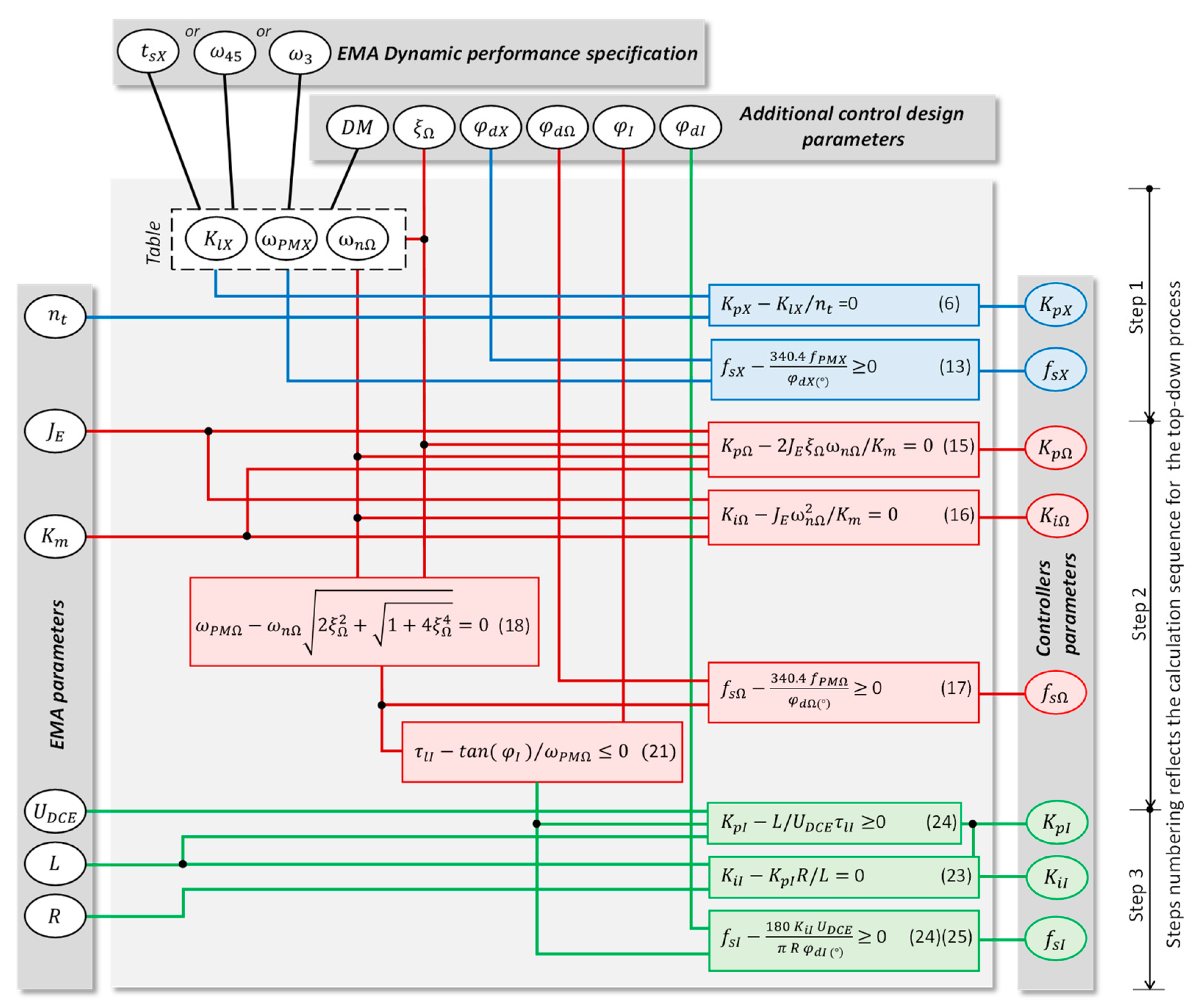
All these results can be represented graphically to summarise the interdependencies among the parameters involved in the design of the EMA position control. This is achieved using the diagram shown in Figure 7.

The blue, red and green blocks use the equations related to the position, speed and current controllers, respectively. A noncausal representation is preferred (nonoriented signal lines) because this enables the calculation causality to be adapted to the current context. This possibility is particularly attractive, e.g., for EMA preliminary sizing when the control hardware is imposed. When read from the top down, the data flow implements the proposed top-down process, where each sequential step from 1 to 3 is dedicated to the setting of a given controller and the specification of the next inner controller. The eight controller parameters (right) are computed given the performance specification and control design choices (top), given the main EMA design parameters (left). When the process is combined with preliminary sizing and optimisation during the early phases of a project, the $J_E$, $L$ and $R$ parameters can be obtained from estimation models, for example, using scaling laws or metamodels [8], from the main design parameters $n_t$, $K_m$ and $U_{DCE}$

3. Illustrative Example

The example of a wingtip, direct-drive, linear flight control actuator used for regional aircraft [19] is used to illustrate the proposed control design. The process is validated through the simulation of an accurate lumped-parameter model of the actuator (control and electromechanical units) and the driven load, which was developed in former studies [20,21].

3.1. Virtual Prototype

The modelled and unmodelled phenomena are summarised in

Table 1. Model used for the virtual validation of the controller design.

	Modelled	Not Modelled
DC link *	Diode and capacitance	Parasitic serial and parallel resistances or capacitance
	Braking resistance, chopper and its control
Three-phase inverter	3 legs, 6 transistors
	Conduction and switching losses
Three-phase PMSM	Motor constant	Cyclic inductance Magnetic saturation Iron losses
	Windings resistance and inductance
	Temperature effects on motor constant and windings resistance
Mechanical transmission *	Mechanical transformation (nut-screw)	Moving body Side loads
	Inertia of rotating and mass of translating assemblies
	Rotational and translational friction with true sticking and effects of speed, load and temperature
	Transmission compliance and backlash (in translational domain)
	End stops
Kinematics to load	Three-bar mechanism (variable lever arm)	Friction and side loads at eye or hinge joints
	Transmission compliance and backlash
Sensors *	Gain, range, dynamics, demodulation, antialiasing, sampling, quantisation, saturation and noise	Offset and thermal drift Hysteresis and nonlinearity
Controller	Discrete, with saturation and antiwindup, time for processing
	BEMF compensation if used, FOC using dq0 model
	Limitation of speed, current and voltage demands (according to motor operating range)
PWM *	Symmetrical triangle carrier, sampling, saturation
	Timing and synchronisation with current loop
Thermal *	All energy losses made temperature-dependent and generating heat	Thermal transients

* See [22,23].

. The high-fidelity model is implemented and simulated in the Simcenter-AMEsim (2020.1, Imagine, Roanne, France) environment. It involves 75 state variables, no implicit variable and +200 parameters. Iron losses and magnetic saturation at the motor are not modelled as they are not significant in this application. Any energy loss is made sensitive to temperature, enabling isothermal simulations to be run for various operating temperatures. Given the dynamics in presence and the sampling/switching frequencies, a 1 s simulation with integration accuracy of 10⁻⁷ typically takes a 290 s CPU on a 64-bit personal computer (Intel Core I7-8550U CPU at 1.8 GHz).

3.2. Virtual Validation

The EMA position controller is virtually validated using a bottom–up incremental approach that follows the real validation process, i.e., the integration branch of the V-model of product lifecycle [3]. The operation of every (simulated) element of the EMA (motor, inverter, measurement chains and mechanical transmission) has been virtually validated, as should be done with partial tests for the real elements. The current loop is validated first, followed by the speed loop and finally the position loop.

The controllers have been designed with the following allocation of the parasitic phase lag because of digital implementation: 5° for the position loop, 10° + 10° for the speed loop and 20° for the current loop.

The loops are excited to assess both pursuit and rejection performances on the same response plot. As numerical simulation naturally provides time responses, a demand step is applied first, followed by a disturbance step. To make the virtual validation realistic, a random noise is introduced on each measured quantity, typically very few percent of the maximal or rated values. The time responses given in this section have been plotted using the realistic magnitudes that were identified during real tests of the power and signal electronics: 4% of the maximal RMS phase current, 3% of the rated rotor speed, 5° for the rotor angle and 6% of LVDT secondary voltage magnitude. Particular attention is also paid to the effect of nonlinearities and unmodelled dynamics on the performance expected from the linear continuous control model. In this attempt, the responses are analysed for various step magnitudes. High magnitude leads to saturations as a result of power and signal limitations. Medium magnitude generally enables the EMA to operate far from hard nonlinear effects and static imperfections. Very low magnitude points to the influence of static imperfection such as quantisation, breakaway friction and backlash.

The dimensionless responses are presented to provide on a single figure the demand, the response of the linear continuous control model and the response of the high-fidelity, nonlinear, high-order model. In the responses provided for the high-fidelity model, the EMA is assumed to operate at room temperature. The excitation magnitudes are referred to the rated values and to the noise magnitude (before the antialiasing filter). The time values are hidden for confidentiality. However, it can be mentioned that the time ranges of Figure 8, Figure 9 and Figure 10 are in the ratio 1:8:100, respectively, to indicate the relative dynamics of the current, speed and position loops.

3.2.1. Current Loop

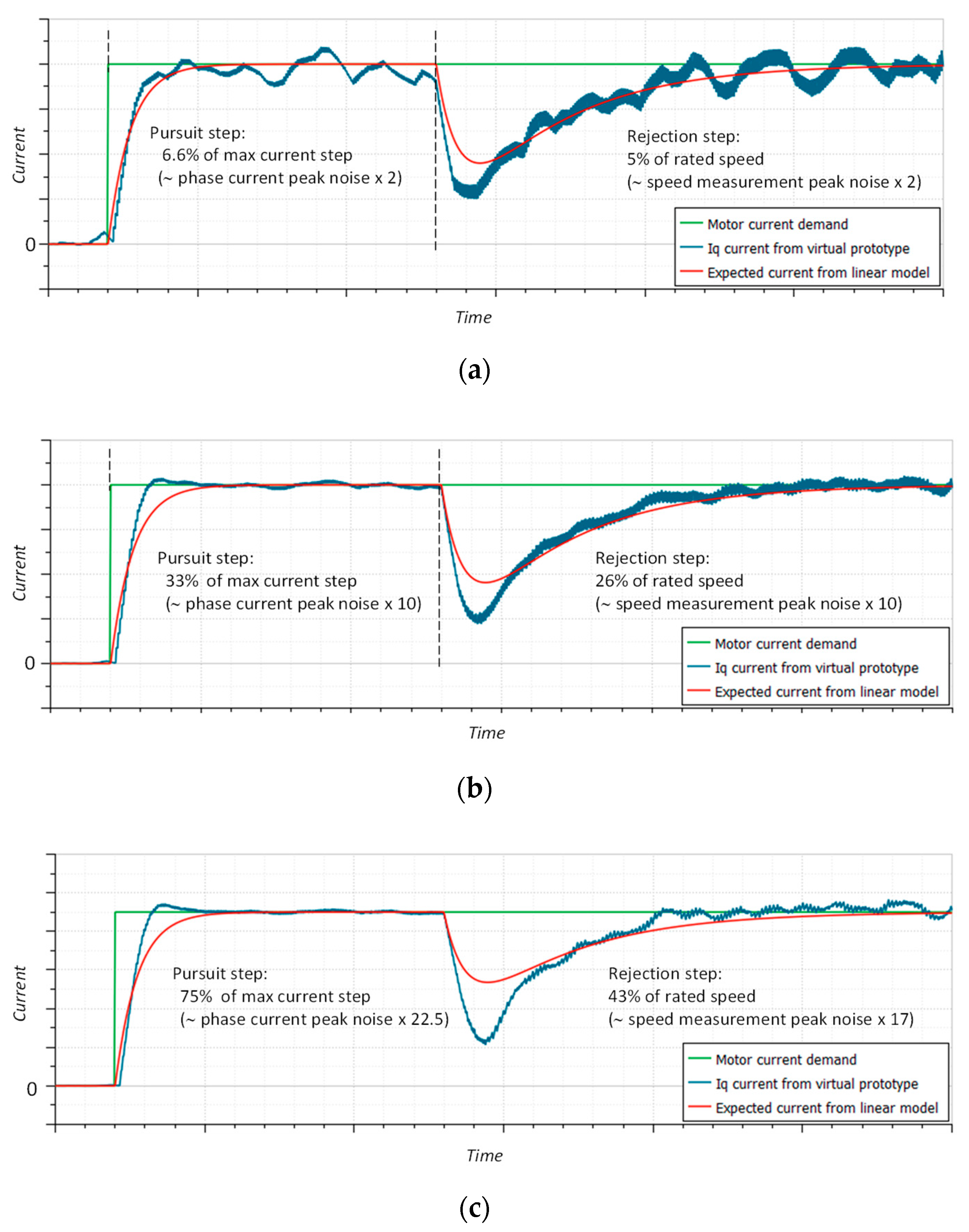
To obtain the current loop responses, the speed and position loops are opened. The motor is tested without connection to the nut-screw while externally imposing the rotor angular velocity. A current step demand ($I_m^{*}$ or $I{ }_q^{*})$ is applied first with the rotor blocked, followed by a motor speed step disturbance ${\mathsf{\Omega }}_m$. The response of the linear continuous control model is obtained from the last transfer function of

Table A1. Current loop model and analysis in continuous time domain.

Constitutive Equations
Pulse width modulation	$U_m=m{U}_{DCE}$ $I_m=\frac{1}{m}{I}_{DCE}$	Variables: $U_m$ motor voltage, $I_{DCE}$ supply current, $I_m$ motor current, $m$ modulation ratio Parameters: $U_{DCE}$ equivalent line to line voltage
Motor windings electrical circuit	$U_m=E+R{I}_m+Ls{I}_m$	Variables: ${\mathsf{\Omega }}_m$ motor shaft angular velocity, $s$ Laplace variable, $E$ motor BEMF Parameters:$R$ motor windings resistance, $L$ motor windings inductance
P-I current controller	$m=\left(K_{pI}+K_{iI}/s\right)\left(I_m^{*}-I_m^{\prime }\right)$	Parameters: $K_{pI}$ current loop proportional gain, $K_{iI}$ current loop integral gain Variables: $I_m^{*}$ motor current setpoint, $I_m^{\prime }$ measured current (equals the real current $I_m$ if the measurement is perfect)
Current Open-Loop Transfer
$I_m=\frac{\frac{K_{iI}{U}_{DCE}}{s}\left(1+{\tau }_{CI}s\right)\left(I_m^{*}-I_m\right)-E}{R\left(1+{\tau }_{e}s\right)}$		Motor electric time constant ${\tau }_e=L/R$ Current controller time constant ${\tau }_{CI}=K_{pI}/K_{iI}$
Current Closed-Loop Transfer (P Control Only)
$I_m=\frac{1}{R\prime }\frac{K_{pI}{U}_{DC}{I}_m^{*}-E}{1+\tau {\prime }_{e}s}$		Apparent windings resistance $R^{\prime }=R+K_{pI}{U}_{DCE}$ Apparent electric time constant ${\tau }_e^{\prime }=L/\left(R+K_{pI}{U}_{DCE}\right)$
Current Closed-Loop Transfer (P-I Control, ${\mathbf{\tau }}_{\mathbf{C}\mathbf{I}}\mathbf{=}{\mathbf{\tau }}_{\mathbf{e}}$)
$I_m=\frac{1}{1+{\tau }_{lI}s}\left(I_m^{*}-\frac{{\tau }_e/K_{pI}{U}_{DCE}}{\left(1+{\tau }_{e}s\right)}sE\right)$
Static pursuit gain:		$I_m/I_m^{*}$ = 1
Tracking rejection gain:		$I_m/sE={\tau }_e/K_{pI}{U}_{DCE}$
Denominator time constant (pursuit):		${\tau }_{lI}=L/K_{pI}{U}_{DCE}$
Denominator time constant (rejection):		${\tau }_e$
Controller setting for ${\tau }_{lI}$ target pursuit dynamics:		$K_{pI}=L/{\tau }_{lI}{U}_{DCE}$$,K_{iI}=K_{pI}R/L$

. The responses are displayed in Figure 8.

Figure 8. Time response of the current loop for step excitations: (a) small-magnitude excitations, noise effects magnified; (b) medium-magnitude excitations, operation close to linear; and (c) large-magnitude excitations, close to internal saturation.

Figure 8. Time response of the current loop for step excitations: (a) small-magnitude excitations, noise effects magnified; (b) medium-magnitude excitations, operation close to linear; and (c) large-magnitude excitations, close to internal saturation.

This figure elicits the following comments:

• The responses of the controlled virtual prototype globally agree well with the responses expected from the linear model and control strategy.
• As anticipated, stability is degraded by sampling and antialiasing but remains acceptable given the active management of this effect in the control design process and the 10° ${\phi }_{dI}$ allocation.
• Figure 8a shows the influence of the current and speed measurement noises. Although the current demand is only twice the peak noise of the current measurement prior to the antialiasing filter, the current response remains globally stable.
• Under medium-magnitude excitations (Figure 8b), the relative importance of noises on response decreases.
• Under high-current and high-speed excitations (Figure 8c), the current response to the speed disturbance is affected by a significant ripple. As explained in [24], this effect comes from the tracking error of the rotor position measurement used by the dq0 transforms, although this is very fast, which generates an alias I_d current proportionally to the I_q current demand.

3.2.2. Speed Loop

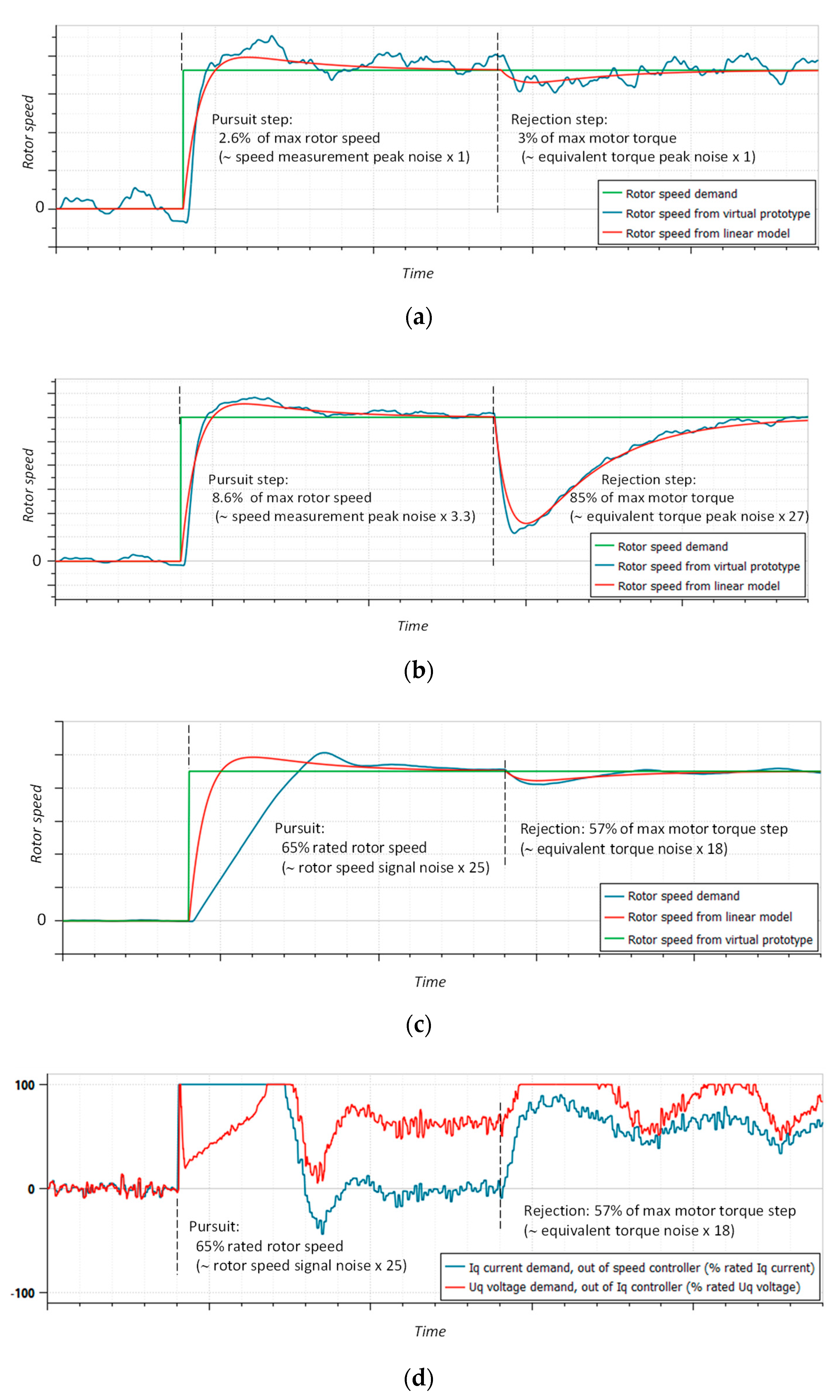
For the speed loop test, the position loop is opened and the translating part of the nut-screw is removed. A rotor speed step demand ${\mathsf{\Omega }}_m^{*}$ is applied first for a free rotor shaft, followed by a step disturbance torque $T_L$ applied to the rotating part of the nut-screw. The response of the continuous linear control model is obtained from the last transfer function of Table A2. The most relevant time responses are displayed in Figure 9, which elicits the following comments:

• Once again, the responses of the controlled virtual prototype globally agree well with the response expected from the linear model and control strategy.
• Even when the excitation magnitudes are only a few times the measurement noise before the antialiasing filter (Figure 9a), the expected dynamics and average response are still satisfactory.
• There is very little difference between the simulated and expected responses for medium-excitation magnitudes when they do not lead to saturation (Figure 9b).
• For high magnitudes of excitations (Figure 9c), the current and the voltage demand saturate for a long time during transients (Figure 9d). This makes the EMA operate temporarily in an open loop. At the end of the saturating phases, the normal control is recovered with high rapidity and stability. The absence of an excessive overshoot or limit cycle proves the correct setting and efficiency of the antiwindup function of the P-I controllers, implemented using the back calculation and tracking scheme [25].

Figure 9. Time response of the speed loop for step excitations: (a) small-magnitude excitations, noise effects magnified; (b) medium-magnitude excitations, at the limit of saturation; (c) large-magnitude excitations, introducing long saturation of the current and modulation ratio; and (d) the speed and current controller outputs for large-magnitude excitations.

Figure 9. Time response of the speed loop for step excitations: (a) small-magnitude excitations, noise effects magnified; (b) medium-magnitude excitations, at the limit of saturation; (c) large-magnitude excitations, introducing long saturation of the current and modulation ratio; and (d) the speed and current controller outputs for large-magnitude excitations.

3.2.3. Position Loop

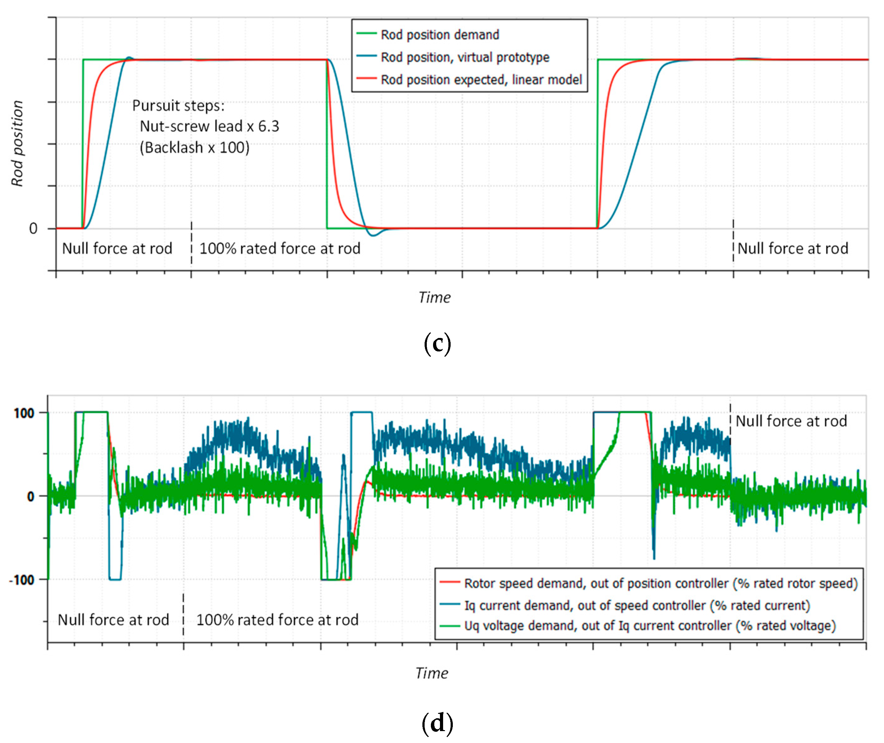
The simulations are run with all control loops active. According to the customer’s specification for the validation of the EMA performance, a pure mass equivalent to the reflected mass of the driven load is attached to the EMA rod. The rod position step setpoint $X_L^{*}$ is applied first from rest at the null position, without any external force.

To better highlight the combined effect of EMA friction and backlash, the external disturbance force $F_L$ is then applied at the EMA rod, without any change in the position demand, as two opposite and consecutive steps. The response of the continuous linear control model is obtained by a simulation of the speed closed-loop model combined with Equations (5) and (6). The most relevant time responses are displayed in Figure 10:

• At a very low magnitude of rod position demand (twice the EMA internal backlash), the response is still smooth and close to that expected from the linear model (Figure 10a). Logically, the combination of Coulomb friction, backlash and I control (speed and current loops) generates a limit cycle, albeit with a very low magnitude (<10% of the backlash).
• Even in the presence of backlash, the rod force step is rejected with the same dynamics as that of the linear model (Figure 10b). For 100% force, the transient position error does not exceed 155% of the backlash or 10% of the nut-screw lead. This excellent capability of external force disturbance confirms the soundness of the proposed approach, which is intended to maximise the position loop gain for a given ${\xi }_{\mathsf{\Omega }}$.
• The position response under saturating excitations is illustrated by Figure 10c,d. The position demand is a pulse whose magnitude is just lower than the actuator stroke. A 100% rated rod force is applied to assess the position response under aiding and opposite loads. The influence of speed, current and voltage saturations clearly appears in Figure 10c, where the position response becomes unable to meet the expected dynamics. When the controllers leave the saturation domain, control is rapidly recovered in the linear domain with very few oscillations.

Figure 10. Time response of the position loop for step excitations: (a) small-magnitude excitations, noise effects magnified; (b) rejection of rod force disturbance, null position demand; (c) large-magnitude excitations, introducing long saturation of the current and modulation ratio; and (d) controller outputs for large-magnitude excitations.

Figure 10. Time response of the position loop for step excitations: (a) small-magnitude excitations, noise effects magnified; (b) rejection of rod force disturbance, null position demand; (c) large-magnitude excitations, introducing long saturation of the current and modulation ratio; and (d) controller outputs for large-magnitude excitations.

4. Discussion

Within the nonsaturating domain of operation, two main nonlinear effects act as disturbances in the linear model that is used for control synthesis. It is important to relate the excellent robustness of the position control to these unmodelled effects and to their magnitude: in the reported validation, the EMA internal backlash is 6.3% of the nut-screw lead, while the load-independent friction force represents 3% of the EMA rated force. At the rated output force, this percentage rises to 12.4% under the contribution of the load-dependent friction. When they are expressed as their equivalent at the EMA rod level, the motor rotor inertia is 44 times greater than that of the driven load.

Besides this particular example, it is worth addressing more general comments:

As shown by Equation (8), the $K_{XF}$ rod position sensitivity to the rate of external load is inversely proportional to $K_{pX}{\omega }_{n\mathsf{\Omega }}^2$. Given the proposed control design process, the selection of ${\xi }_{\mathsf{\Omega }}$ can offer a means to act on $K_{XF}$ to meet a given pursuit dynamics.

• For very preliminary control design, it is advised to link the EMA internal parameters (e.g., inertia, nut-screw lead, motor windings resistance) to the EMA top-level specifications (maximal or rated speed and force at rod, along with reliability). This can, for example, be achieved using scaling laws, as proposed in [8]. Combining power and control preliminary designs would then enable more global and automated EMA design exploration and optimisation.
• Two examples have been provided in Section 2.1 to generate the performance charts. As these charts are precalculated once, other types of constraints can be applied and combined, without any need to change the process.
• Although the top-down process is driven by the overall control need, it is worth mentioning that it may output hardware and software specifications that cannot be met because of, for example, a lack of performance, maturity, availability or excessive cost. Therefore, precautions must be taken to check that each subspecification generated can be met in practice. If not, the concerned subspecification has to be replaced by a constraint, and the data flow of the design process has to be revised accordingly. This is enabled by the noncausal representation used in Figure 7.

5. Conclusions

The design of position control of EMAs has been addressed for aerospace safety-critical applications. The focus has been placed on the proposition and implementation of a top-down process requiring very few input data for the design of cascade controllers, when certifiability constraints and design assurance levels welcome common control techniques. This work was primarily intended to enable control considerations to be added to the preliminary sizing phases in order to accelerate the development process. This objective was achieved by several contributions. The first one comes from the generation of charts that link the position control gain to the speed loop dynamics and damping targets, when a position control performance criterion is maximised. For a given loop, the second one consists in determining the control parameters, the numerical implementation and the specification of the following loop, in a formal and simple way which calls upon a minimal number of EMA parameters. The third contribution lies in the graphical representation that synthetises in a noncausal way the interdependencies between the control specifications, the EMA key design parameters, the control choices and the controller parameters. The proposed process has been virtually validated using a very detailed high-fidelity model of the EMA. The EMA responses derived from the virtual testbench have shown the efficiency of the proposed process, even in the presence of significant noise, saturation, friction and backlash, which are unmodelled in the linear models used for control synthesis.

References

- Gonzalez, C.M. Engineering Refresher: The Basics and Benefits of Electromechanical Actuators. Available online: https://cdn.baseplatform.io/files/base/ebm/machinedesign/document/2019/04/machinedesign_15522_electromechanical.pdf (accessed on 8 February 2022).
- O’dwyer, A. Handbook of PI and PID Controller Tuning Rules, 3rd ed.; Imperial College Press: London, UK, 2009. [Google Scholar]
- Incose Systems Engineering Handbook: A Guide for System Life Cycle Processes and Activities, 4th ed.; Wiley-Blackwell: San Diego, CA, USA, 2015.
- Ali, Z.A.; Han, Z. Maneuvering Control of Hexrotor UAV Equipped With a Cable-Driven Gripper. IEEE Access 2021, 9, 65308–65318. [Google Scholar] [CrossRef]
- Fadel, M. Position Control for Laws for Electromechanical Actuator. In Proceedings of the 2005 International Conference on Electrical Machines and Systems, Nanjing, China, 27–29 September 2005; pp. 1708–1713. [Google Scholar] [CrossRef]
- Zhang, M.; Li, Q. A Compound Scheme Based on Improved ADRC and Nonlinear Compensation for Electromechanical Actuator. Actuators 2022, 11, 93. [Google Scholar] [CrossRef]
- Khanh, N.D.; Kuznetsov, V.E.; Lukichev, A.N.; Chung, P.T. Adaptive Control of Electromechanical Actuator Taking into Account Nonlinear Factors Based on Exo-model. In Proceedings of the 2022 Conference of Russian Young Researchers in Electrical and Electronic Engineering (ElConRus), St. Petersburg, Russia, 25–28 January 2022; pp. 803–807. [Google Scholar] [CrossRef]
- Budinger, M. Preliminary design and sizing of actuation systems. In Mechanical Engineering [physics.class-ph]; UPS Toulouse: Toulouse, France, 2014. [Google Scholar]
- Wu, S.; Bo, Y.; Jiao, Z.; Shang, X. Preliminary design and multi-objective optimization of electro-hydrostatic actuator. Proc. Inst. Mech. Eng. Part G J. Aerosp. Eng. 2010, 231, 1258–1268. [Google Scholar] [CrossRef]
- Vaculik, S.A. A Framework for Electromechanical Actuator Design. Ph.D. Thesis, The University of Texas at Austin, Austin, TX, USA, May 2008. Available online: https://repositories.lib.utexas.edu/bitstream/handle/2152/18161/vaculiks84501.pdf?sequence=2&isAllowed=y (accessed on 8 February 2022).
- Krishnan, R. Permanent Magnet Synchronous and Brushless DC Motor Drives; Taylor and Francis Group: Boca Raton, FL, USA, 2010. [Google Scholar] [CrossRef]
- Sang-Hoon, K. Electric Motor Control; Elsevier: Amsterdam, The Netherlands, 2017. [Google Scholar] [CrossRef]
- Dee, G.; Vanthuyne, T.; Alexandre, P. An electrical thrust vector control system with dynamic force feedback. In Proceedings of the 3rd International Conference on Recent Advances in Aerospace Actuation Systems and Components, Toulouse, France, 13–15 June 2007; pp. 75–79. [Google Scholar]
- Landau, I.D. Identification et Commande des Systèmes; Hermes: Paris, France, 1988. [Google Scholar]
- Krishnan, R. Electric Motor Drives: Modeling, Analysis, and Control; Prentice Hall: Upper Saddle River, NJ, USA, 2001. [Google Scholar]
- Crowder, R. Electric Drives and Electromechanical Systems Applications and Control, 2nd ed.; Elsevier: Oxford, UK, 2020. [Google Scholar]
- Maré, J.-C. Friction modelling and simulation at system level—Considerations to load and temperature effects. IMechE Part I J. Syst. Control. Eng. 2015, 229, 27–48. [Google Scholar] [CrossRef]
- Arriola, D. Model-based Design and Fault-tolerant Control of an Actively Redundant Electromechanical Flight Control Actuation System. Ph.D. Thesis, Technical University Hamburg, Hamburg, Germany, 2019. [Google Scholar]
- Dimino, I.; Gallorini, F.; Palmieri, M.; Pispola, G. Electromechanical Actuation for Morphing Winglets. Actuators 2019, 8, 42. [Google Scholar] [CrossRef] [Green Version]
- Wang, L. Force Equalization for Active/Active Redundant Actuation System Involving Servo-Hydraulic and Electro-Mechanical Technologies. Ph.D. Thesis, INSA, Toulouse, France, December 2012. Available online: http://www.theses.fr/2012ISAT0038/document (accessed on 8 February 2022).
- Karam, W. Générateurs de Forces Statiques et Dynamiques à Haute Puissance en Technologie Électromagnétique. Ph.D. Thesis, INSA, Toulouse, France, November 2007. Available online: http://eprint.insa-toulouse.fr/archive/00000182/http://www.theses.fr/2007ISAT0035/document (accessed on 8 February 2022).
- Fu, J.; Maré, J.-C.; Fu, Y. Modelling and simulation of flight control electromechanical actuators with special focus on model architecting, multidisciplinary effects and power flows. Chin. J. Aeronaut. 2017, 30, 47–65. [Google Scholar] [CrossRef] [Green Version]
- Fu, J.; Maré, J.-C.; Yu, L.; Fu, Y. Multi-level virtual prototyping of electromechanical actuation system for more electric aircraft. Chin. J. Aeronaut. 2018, 31, 889–913. [Google Scholar] [CrossRef]
- Maré, J.-C. Recent Experiences in Extending the Scope of EMA Simulation for Virtual V&V. In Proceedings of the SAE A-6B3 Panel, Spring Meeting, Virtual, 28 April 2021; Available online: https://www.sae.org/works/meetingminuteResources.do?comtID=TEAA6&resourceID=867983 (accessed on 8 February 2022).
- Åström, K.J. Advanced Control Methods: Survey and Assessment of Possibilities. In Advanced Control in Computer Integrated Manufacturing: A Control Engineer’s View; Morris, H.M., Kompass, E.J., Williams, T.J., Eds.; Purdue University: West Lafayette, IN, USA, 1987. [Google Scholar]
- Maré, J.-C. Practical Considerations in the Modelling and Simulation of Electromechanical Actuators. Actuators 2020, 9, 94. [Google Scholar] [CrossRef]
- Mohan, N.; Undeland, T.M.; Robbins, W.P. Power Electronics: Converters, Applications and Design, 1st ed.; Wiley: Hoboken, NJ, USA, 1989. [Google Scholar]
Figure 1.
Cascade control of EMAs (notations are detailed in the Appendix A and Appendix B, full arrows and half arrows highlight the signal and power flows, respectively).
Figure 2.
Block-diagram representation of the equivalent linear control model of the EMA to control (see Appendix A and Appendix B for details).
Figure 3.
I-P speed controller obtained by filtering the speed setpoint (continuous-time domain).
Figure 4.
Performance indicators for position control for the fastest closed-loop step response without overshoot using dimensionless variables: (a) loop gain, settling time and phase margin; (b) performance indicators in the frequency domain; (c) frequency for the phase margin; and (d) closed-loop rapidity versus loop gain.
Figure 5.
Performance indicators of position control with the P-I implementation of the speed controller giving the fastest response time under a purely real negative closed-loop poles constraint.
Figure 6.
Friction force in EMAs: (a) the influence of temperature on friction torque for a geared EMA at a rated output torque, calculated from harmonic drive efficiency data (size 14, ratio 100) [17]; (b) the influence of speed and load at room temperature (demonstration EMA sized for the Airbus A320 aileron–gear drive, ball screw, no preload) [18].
Figure 7.
Noncausal representation of the interdependence among parameters for the design of the EMA position control.