Article

Trajectory Tracking Based on Active Disturbance Rejection Control for Compound Unmanned Aircraft

National Key Laboratory of Rotorcraft Aeromechanics, Nanjing University of Aeronautics and Astronautics, Nanjing 210016, China
*
Author to whom correspondence should be addressed.
Aerospace 2022, 9(6), 313; https://doi.org/10.3390/aerospace9060313
Submission received: 25 April 2022 / Revised: 28 May 2022 / Accepted: 6 June 2022 / Published: 9 June 2022
(This article belongs to the Collection Unmanned Aerial Systems)

Abstract

:
The compound unmanned aircraft is provided with three primary flight modes, which are helicopter flight mode in low forward speed flight, airplane flight mode in high forward speed flight and transition flight mode in middle forward speed flight. For the different flight modes, an appropriate flight control law is the need to ensure good flying qualities. In this paper, a trajectory tracking control system based on the active disturbance rejection controller (ADRC) for the compound unmanned aircraft is proposed to adapt the full flight modes. A flight dynamics model and a Simulink simulation model of the compound unmanned aircraft are developed. The transition flight control strategy is analyzed and synthesized to meet the requirement of control strategy in the full flight modes. The internal uncertainties and external disturbance of the UAV are estimated with an extended state observer to compensate control input. A genetic algorithm-particle swarm optimization (GA-PSO) algorithm is utilized to optimize the controller parameters. The simulation of route tracking and spiral climb with different flight modes is conducted, which demonstrates the tracking ability, interference rejection, robustness and effectiveness of the developed controller in the full flight modes.

1. Introduction

The compound unmanned aircraft has the hover capability of a helicopter and the high velocity forward flight capability of an airplane [1], which is different from a traditional unmanned helicopter and has variable flight modes due to the addition of wings and propellers. The structure of a compound unmanned aircraft is complex and its control variables are redundant, so that the flight dynamics model is more complicated and the uncertain factors are manifold [2,3]. In order to ensure the stable flight of compound unmanned aircraft during entire flight envelope, it is necessary to design the trajectory tracking control system using robust nonlinear controller.
In the recent years, advances in the field of automatic flight controls system for all kinds of unmanned aerial vehicle (UAV) have been made. The compound unmanned aircraft is an UAV with multi-input multi-output (MIMO) nonlinear system [4,5], whose dynamical models are difficult to derive and implement because the complicated higher order polynomial or differential equations are needed to fully characterize the controlled plant. In some studies, a linearized mathematical model of UAV is usually established by the linearization theory of small disturbance [6], which is integrated with channel laws to realize the simulation and verification of flight control system. For example, Seema et al. designed yaw and pitch controllers for the twin rotor MIMO system (TRMS) based on fractional order PID controller (FOPID) [7]. Hernando et al. presented the design of an adaptive fuzzy Proportional-Integral-Derivative (PID) controller to regulate the elevation, pitch and travel angles of a helicopter with three degrees of freedom [8]. Halbe et al. proposed a trajectory controller based on sliding mode control [9]. A trajectory linearization method combined with sliding mode disturbance observer is applied to design a trajectory tracking controller for an unmanned helicopter by Tang et al. [10]. A backstepping control algorithm for the autonomous landing of a quadrotor on a moving mobile platform was proposed by Ghommam et al. [11]. Many other control algorithms were designed based on linear control theory and linearized model of small disturbance, whose tracking ability, interference rejection and robustness are verified with digital simulation.
Though linear controllers are easily designed and implemented, they are valid within a small subset of the entire flight envelope. The capability of linear controllers is limited [12,13]. It is difficult for the linear controllers to accurately control an actual UAV with the internal uncertainties and external disturbance [14,15]. As the UAV control accuracy requirements improve, it is necessary to design flight control system with a robust nonlinear controller.
The active disturbance rejection control theory [16] proposed by Han can be applied to treat the internal uncertainties and external disturbance as total disturbance of system. The extended state observer of ADRC can estimate total disturbance and compensate the control law in real time [17,18]. Using this method, a yaw channel controller with linear ADRC for high-performance attitude tracking of an unmanned helicopter was proposed by Li et al. [19]. A control strategy based on ADRC, and improved sliding mode control (ISMC) algorithms were proposed to stabilize the helicopter load system by Duan et al. [20]. An active disturbance rejection controller for the Trex 600 unmanned helicopter was designed by Dai et al. [21]. The ADRC with adaptive radial basis function neural network was proposed by Shen et al. [22]. The simulation of these designs indicates that the stability, robustness, anti-disturbance and tracking performance of ADRC are better than those of PID controller. Although the control effect of ADRC is excellent, the number of its difficultly tuned parameters are many. It is necessary to apply the optimization algorithm to tune these control parameters. A particle swarm optimization algorithm (PSO) was proposed to optimize the parameters in the nonlinear state error feedback part of the ADRC by Chen et al. [23]. A control parameter optimization approach used in a novel swarm intelligence algorithm of small, unmanned helicopters was proposed Zhang et al. [24]. Huang et al. applied the double-chains quantum genetic algorithm to optimize the parameters of ADRC [25]. A bacterial foraging optimization-flower pollination algorithm (BFO-FPA) was developed by Shen et al. for tuning ADRC parameters [26]. All the above optimization algorithms have good application simulation results. In this paper, the genetic algorithm-particle swarm optimization (GA-PSO) is developed to optimize the ADRC parameters, which reduces the parameter tuning difficulty.
This paper is outlined as follows: in Section 2, a nonlinear flight dynamics model is established and a flight control strategy is designed. Then the active disturbance rejection controller is designed and the trajectory tracking control system is developed. In Section 3, the GA-PSO is developed to optimize the ADRC parameters. In Section 4, the simulation results and the performance evaluation of the proposed scheme are given, followed by conclusions in Section 5.

2. Design of Trajectory Tracking Control Law

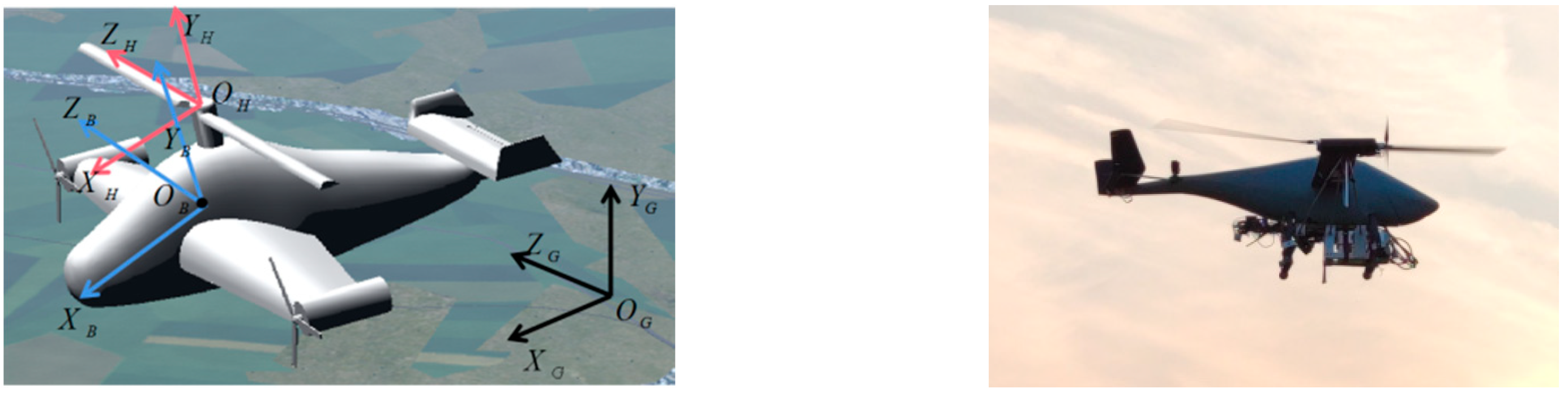
2.1. Flight Dynamics Model

The compound unmanned aircraft is shown in Figure 1. It is composed of a main rotor, propellers, wings, horizontal tail, vertical tails and fuselage. It can realize hovering, high-speed cruise and other maneuvering flights. There are three different flight modes, namely helicopter flight mode, transition flight mode and airplane flight mode. The actual flight would convert between different flight modes according to the flight mission situation. The main parameters of the UAV are shown in Table 1.
The flight dynamics equation of the compound unmanned aircraft is [27]:
V ˙ = F / m - Ω V
S ˙ = I - 1 M - I - 1 Ω I S
α ˙ = E S
P ˙ = R E B V
where V = [ u v w ] T is the linear velocity; S = [ p q r ] T is the angular rate; α = [ ϕ θ ψ ] T is the Euler angle; P = [ X Y Z ] T is position vector in ground coordinate; m is the mass of the whole machine; F is the resultant force of components, including gravity; M is the resultant moment of components; I is the moment of inertia matrix; Ω, E and REB are the cross product vector operator, the conversion matrix from angular velocity to Euler angular velocity and the conversion matrix from airframe coordinate to ground coordinate, respectively, namely:
Ω = [ 0 - r q r 0 - p - q p 0 ]
E = [ 1 s i n f t a n 2 θ c o s f 0 c o s f - s i n f 0 s i n f / c o s θ c o s f / c o s θ ]
R E B = [ c o s θ c o s ψ s i n θ s i n ψ c o s ψ - c o s f s i n ψ s i n θ c o s f c o s ψ + s i n f s i n θ c o s θ s i n ψ s i n θ s i n f s i n ψ + c o s f c o s ψ s i n θ c o s f s i n ψ - s i n f c o s ψ - s i n θ s i n f c o s θ c o s f c o s θ ]

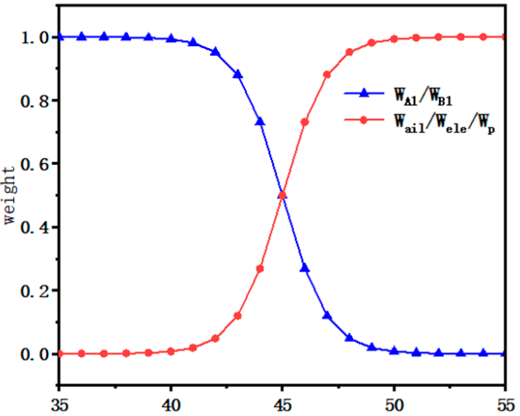
2.2. Control Strategy Design

The compound unmanned aircraft has multiple control mechanisms, including rotor collective pitch, lateral cyclic pitch, longitudinal cyclic pitch, rotor speed, propeller speed, ailerons and elevator. The control variables are more than control channels; thus, the control variables are redundant. The redundant control variable allocation design, that is, the control strategy design, is used to realize different flight modes based on the analysis of the UAV flight dynamics.
It is the helicopter flight mode that the forward speed is less than 35 m/s. The aerodynamic force and torque which are used to drive the movement of a UAV are provided by the rotor and a pair of propellers. The vertical velocity, forward velocity, lateral force, pitch moment and roll moment are controlled by the collective pitch, the lateral and longitudinal cyclic pitch. The yaw moment is achieved by controlling the propellers. The work of propellers not only balances the anti-torque of the rotor but also realizes yaw angle control. In this flight mode, the ailerons and elevator are not used to control the UAV. The UAV can realize typical flight tasks such as vertical take-off and landing, hovering, turning, flying backward and low speed forward flying.
It is the airplane flight mode that the forward speed is more than 55 m/s. The aerodynamic force and torque which are used to drive the movement of UAV are provided by a pair of propellers, wings, ailerons and elevator. The propeller control is used to provide forward velocity and yaw moment. The ailerons control the roll moment, and the elevator controls the pitch moment. The vertical velocity is mainly provided with the wings and its force value is determined by the flight speed. In this flight mode, the lateral and longitudinal cyclic pitch of the rotor are not used to control the UAV, and the collective pitch can be assisted in the vertical velocity control. The rotor anti-torque is still balanced by differential speed of propellers. Typical flight tasks, such as high-speed forward flying, climb, coordinated turning, etc., can be realized.
It is the transition flight mode that the forward speed is 35 m/s–55 m/s. The aerodynamic force and torque which are used to drive the movement of UAV are provided by rotor, propellers, wings and control surfaces. The typical flight task during this mode is the transition from the helicopter flight mode to the airplane flight mode. The control and aerodynamic changes in the transition flight mode are complicated and it is necessary to design a smooth transition control strategy between the helicopter flight mode and the airplane flight mode.
The control strategies for different flight modes are shown in Table 2.
In the transition flight mode between the helicopter flight mode and the airplane flight mode, the control strategies are converted with a variable weight coefficient (0~1). The conversion formula is:
{ A 1 = w A 1 ( v ) δ a B 1 = w B 1 ( v ) δ b δ a i l = w a i l ( v ) δ a δ e l e = w e l e ( v ) δ b δ p = w p ( v ) δ f
where A1 is rotor lateral cyclic pitch, B1 is rotor longitudinal cyclic pitch; δail, δele and δp are aileron control, elevator control and propeller speed respectively; δa, δb and δf are the lateral, longitudinal and forward control, respectively; wA1 and wB1 are the control weights of rotor lateral cyclic pitch and longitudinal cyclic pitch, respectively; wail, wele and wp are the control weights of aileron, elevator and propeller speed, respectively. The distribution of the weight coefficient of each control is converted according to the sigmoid law as shown in Figure 2.

2.3. Active Disturbance Rejection Controller

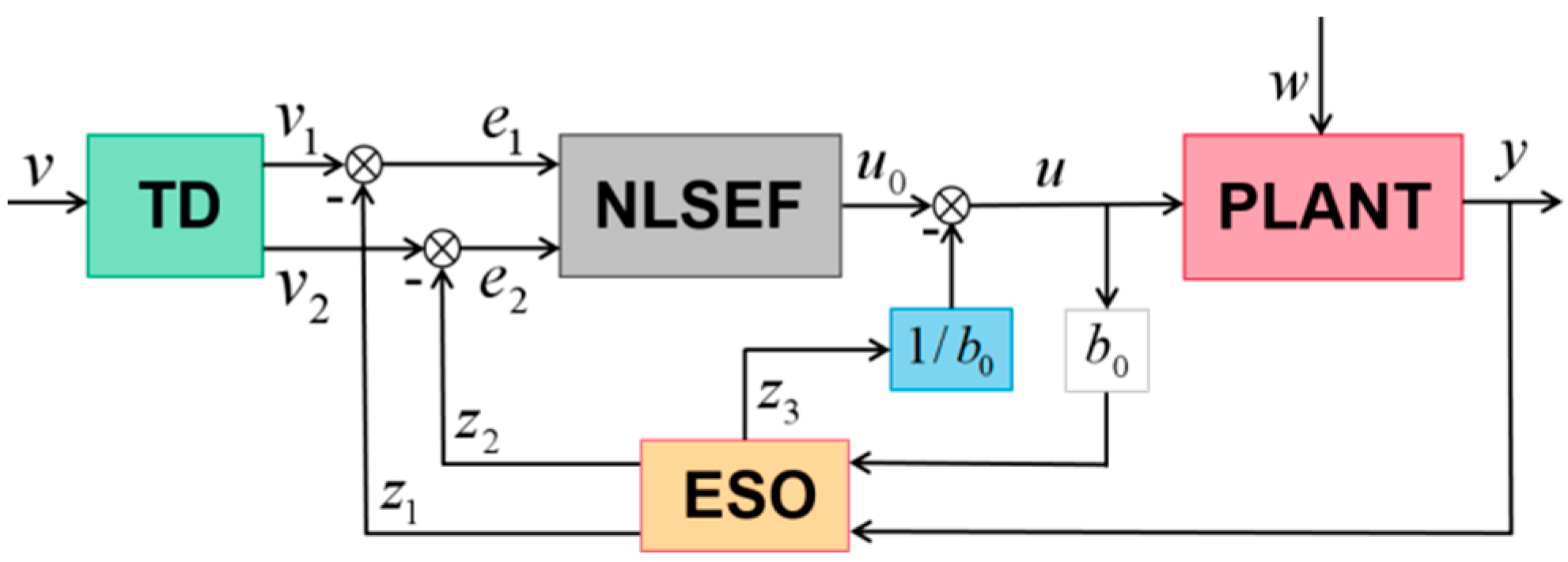
2.3.1. Basic Structure of ADRC

The ADRC is composed of a tracking differentiator (TD), extended state observer (ESO) and nonlinear state error feedback regulator (NLSEF), as shown in Figure 3. TD is used to track the input signal quickly and obtain its differential signal. ESO estimates internal and external disturbances to form a total disturbance. NLSEF is used to compensate the total disturbance and then form the control.

2.3.2. Tracking Differentiator (TD)

The tracking differentiator is arranged as the transition process of the system, expressed as a second-order nonlinear discrete equation:
{ v 1 ( k + 1 ) = v 1 ( k ) + h v 2 ( k ) v 2 ( k + 1 ) = v 2 ( k ) + h × f s t ( v 1 ( k ) - v ( k ) )
where k is the kth sampling, v1 is the tracking signal of the input signal v, v2 is the differential signal of the input signal v, h is the sampling period, r is the speed factor, h and r determine the speed of the tracking speed. fst is the comprehensive function of the fastest control, namely:
{ d = r h d 0 = h d y = v 1 + h v 2 a 0 = d 2 + 8 r | y | a = { v 2 + ( a 0 - d ) 2 s i g n ( y ) , | y | > d 0 v 2 + y / h , | y | d 0 f s t ( v 1 , v 2 , r , h ) = { - r s i g n ( a ) , | a | > d - r a / d , | a | d

2.3.3. Extended State Observer

The second-order nonlinear system equation to be estimated is:
{ x ˙ 1 = x 2 x ˙ 2 = x 3 + b u x ˙ 3 = w ( t ) y = x 1
where u is the input signal, y is the output signal, x1 and x2 are the state variables, x3 is the extended state variable, b is the control gain.
The established expanded state observer is:
{ e = z 1 - y z ˙ 1 = z 2 - β 01 e z ˙ 2 = z 3 - β 02 f a l ( e , α 1 , δ ) + b u z ˙ 3 = - β 03 f a l ( e , α 2 , δ )
f a l ( e , α , δ ) = { e δ α - 1 , | e | δ | e | α s i g n ( e ) , | e | > δ
where zi (i = 1,2,3) is the output signal of the extended state observer, αi (i = 1,2) and β0i (i = 1,2,3) are the step length parameters, fal is nonlinear function.
The extended state observer is used to estimate the total disturbance of the system. The total disturbance estimated by ESO is the control compensation, which converts the nonlinear controlled system into a linear controlled system.

2.3.4. Nonlinear State Error Feedback Regulator (NLSEF)

NLSEF is formed by the nonlinear combination of state deviations corresponding to TD and ESO, namely:
{ e 1 = v 1 - z 1 e 2 = v 2 - z 2 u 0 = β 1 f a l ( e 1 , λ 1 , τ ) + β 2 f a l ( e 2 , λ 2 , τ ) u = u 0 - z 3 / b
f a l ( e , λ , τ ) = { e τ 1 - λ , | e | τ | e | α s i g n ( e ) , | e | > τ
where u0 is the error feedback control, β1 and β2 is the adjustable gain. The function fal has a filtering effect, which can effectively suppress signal chattering.

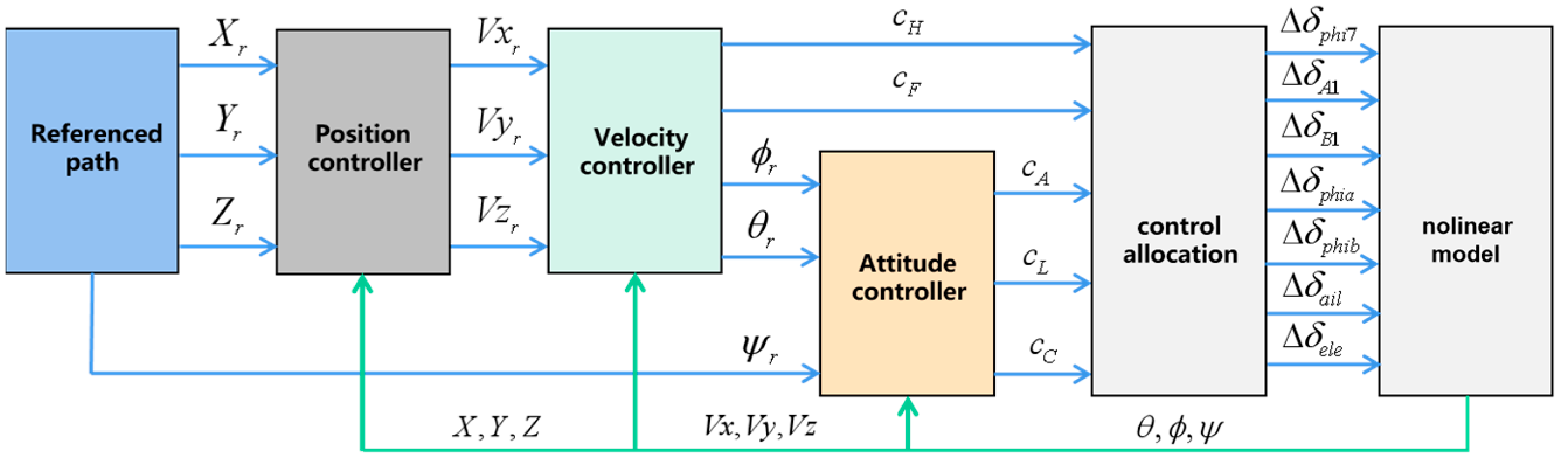
2.4. Trajectory Tracking Control Law

As a controlled object, the dynamics model of the compound unmanned aircraft was represented by the previous. The trajectory tracking control structure design is shown in Figure 4. It is composed of the attitude control loop, the velocity control loop and the position control loop from inside to outside. The controllers in the control loop are designed as second-order active disturbance rejection controllers, which are suitable for different flight modes.

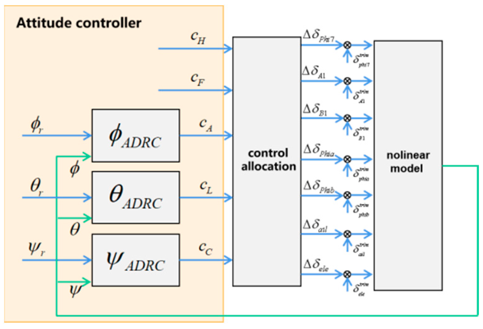
2.4.1. Attitude Control Loop

Equations (2) and (3) can be expressed as:
{ α ˙ = F 1 ( α ) S S ˙ = F 2 ( α , S , V , Ω , w ) + B ( α , S , V , Ω , w ) U c
where w is the external disturbance and Uc = [ c A , c L , c C ] is the virtual control quantity composed of the roll channel, pitch channel and yaw channel. According to Equation (16), the second-order system of state equations can be obtained:
α ¨ = d F 1 d t S + S ˙ F 1 = F 3 S + F 1 ( F 2 + B U c )
where F3 = dF1/dt, F1, F2 and B are the corresponding abbreviation. The total disturbance is expressed as f ¯ α = F 3 S + F 1 ( F 2 + B U c ) - B 0 α U c , then the Equation (17) becomes:
α ¨ = f ¯ α + B 0 α U c
where B0α is the gain matrix of the attitude control. The command of pitch angle and roll angle given by the velocity loop and the command of yaw angle given by the reference command signal are the control inputs of attitude loop. The virtual control quantity Uc = [ c A , c L , c C ] is the output of attitude loop. The control quantities of roll, pitch and yaw channels constitute a single-input single-output relationship with corresponding target attitude angles. The structure of attitude controller is shown in Figure 5.

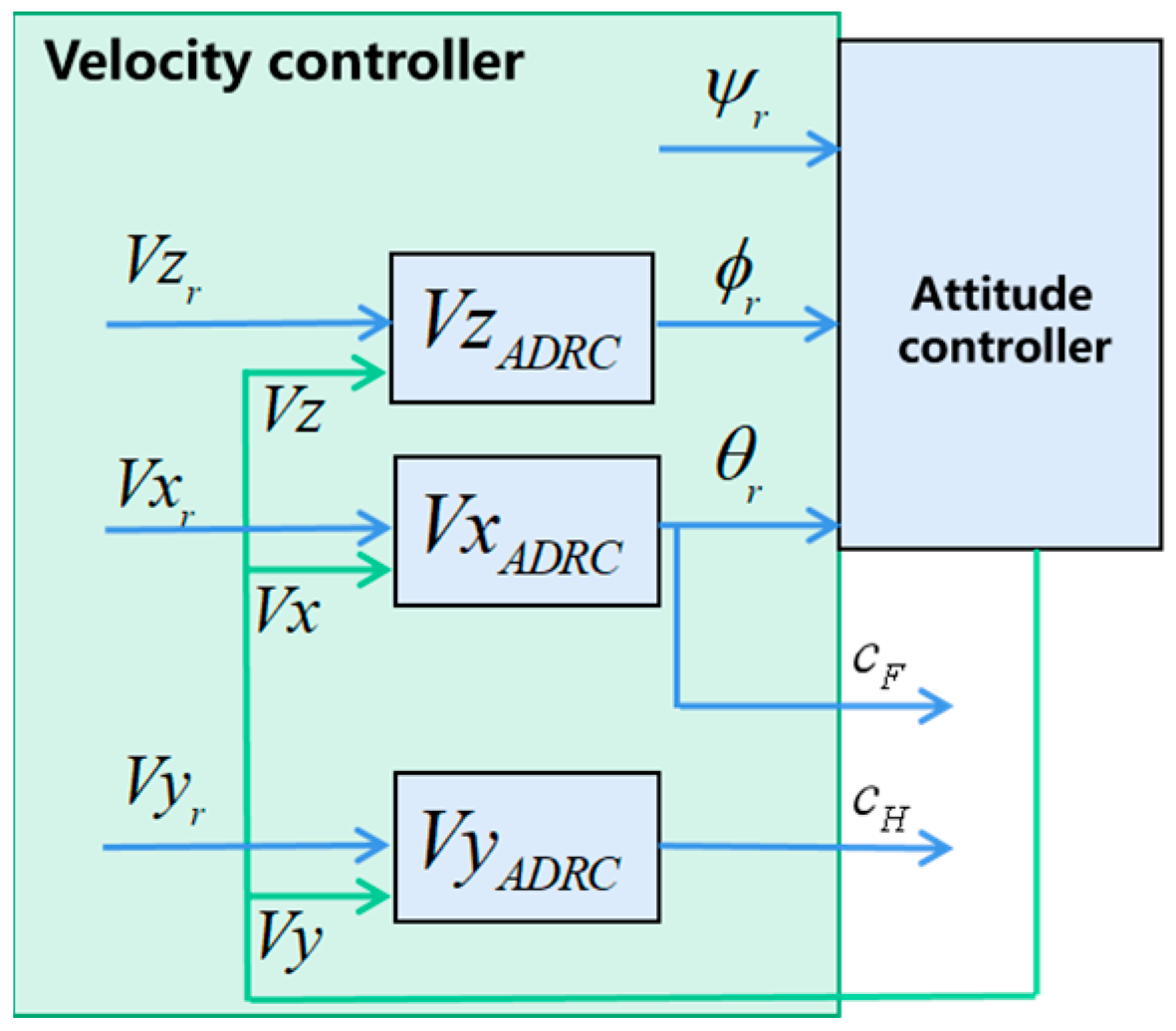
2.4.2. Velocity Control Loop

Equation (1) can be expressed as:
V ˙ = F 4 ( α , S , V , w )
Define the disturbance f ¯ V = F 4 ( α , S , V , w ) B 0 V α ¯ , then:
V ˙ = f ¯ V + B 0 V α ¯
where B0V is the velocity control gain matrix. The velocity controller is in series with the attitude controller in front. The command signals given by the position loop and the virtual control quantity α ¯ = [ ϕ r , θ r , c F , c H ] are the input and output of velocity loop respectively. The structure of the velocity controller is shown in Figure 6.

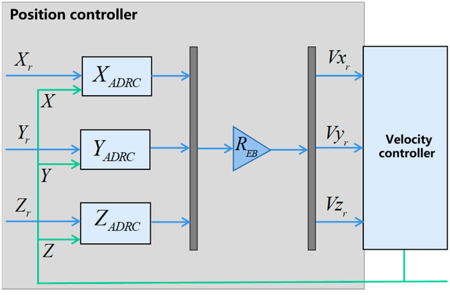
2.4.3. Position Control Loop

Equation (4) can be expressed as:
P ˙ = F 5 ( α , w ) V ¯
Define the disturbance f ¯ P = ( F 5 ( α , w ) - B 0 P ) V ¯ , then:
P ˙ = f ¯ p + B 0 P V ¯
where B0P is the position control gain matrix. The position controller is in series with the velocity controller in front. The reference command signals and the virtual control quantity V ¯ = [ V x r , V y r , V z r ] are the input and output of the position loop, respectively. The structure of the position controller is shown in Figure 7.

3. Control Parameters Tuning

The numbers of the ADRC control parameters are many. It is difficult to tune these control parameters. The GA-PSO is developed to optimize these control parameters.

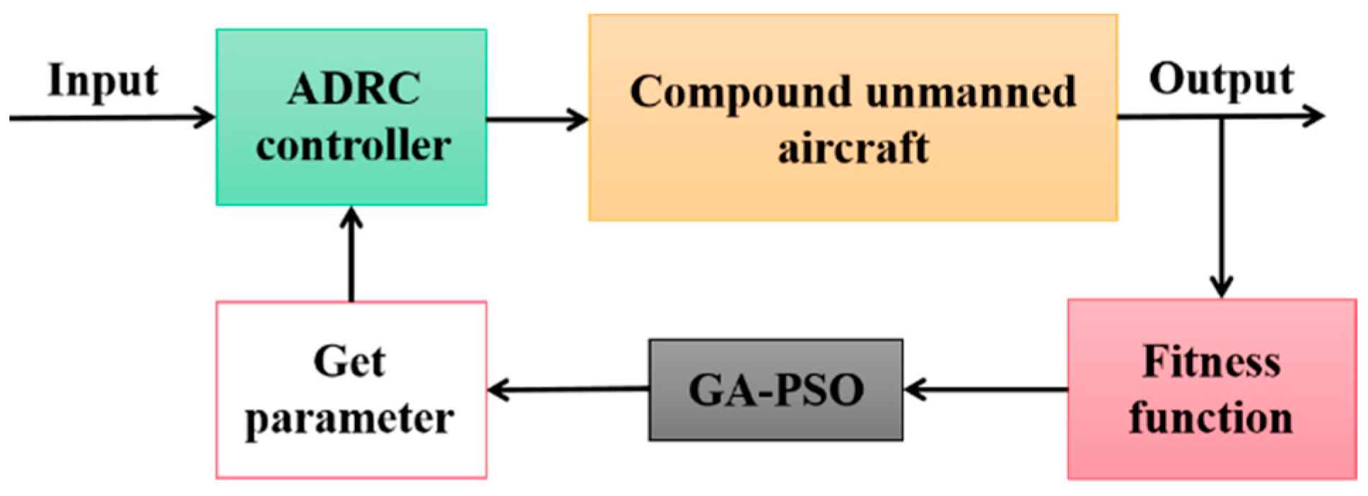
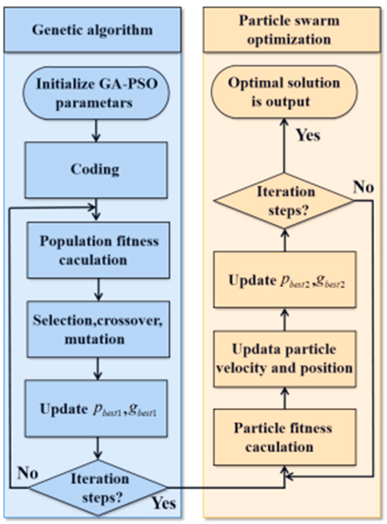
3.1. GA-PSO Algorithm

Genetic algorithm (GA) has strong global search ability which can search multiple points in the population simultaneously. However, GA has poor local optimization ability and poor memory. Particle swarm optimization (PSO) algorithm has the advantages of fast convergence and good memory. However, PSO is easy to fall into the local optimal solution, resulting in low solution accuracy. Therefore, the GA-PSO is proposed, which uses a hierarchical structure to separate global search and local search. GA contributes global search ability at the bottom layer, and at the top layer, PSO performs local search on the elite population optimized from the bottom. Figure 8 is the schematic diagram of the combination of GA-PSO algorithm and ADRC control system, and Figure 9 is the GA-PSO algorithm flow.
The main steps of GA-PSO algorithm are:
  • Initialize parameters of GA-PSO algorithm, including population size, crossover probability, mutation probability and evolution times, etc.
  • Encoding: Generate the initial population which initializes the ADRC parameters. The initial population is substituted into the ADRC control system as a potential solution to simulate and calculate the fitness. The fitness calculation formula is:
    J = i = 1 N 0 t | e i ( t ) Q i ( t ) | d t
    where |ei(t)| is the absolute value of the deviation between target value and output value of the control system. N is the number of control system loops and Qi(t) is the input signal of control loop. The smaller the fitness value, the better the solution.
  • Too large a crossover probability will increase randomness and slow convergence speed of the algorithm, and too large a mutation probability will weaken the inheritance of excellent genes. Too small a crossover probability and too small a mutation probability will cause the algorithm to easily fall into local optimization. To facilitate parameter optimization, sigmoid function is introduced to design adaptive crossover probability and mutation probability, namely:
    { P c = P c min + ( P c max + P c min ) 1 1 + e f i f i a v e P m = P m min + ( P m max + P m min ) 1 1 + e f i f i a v e
    where Pcmax, Pcmin, Pmmax and Pmmin are the maximum and minimum values of crossover and mutation probability, respectively. fi is the current individual fitness and fiave is the average fitness of current population.
  • After the iteration number is satisfied, the elite population obtained from the GA is substituted into the initial population of PSO to calculate the fitness.
  • Update the velocity and position of the particle and determine the optimal solution of current particle and particle swarm. Then update the individual optimal solution Pbest and the global optimal solution Gbest. Too large an update speed affects the accuracy of local search, too small and the algorithm easily falls into local optimization. To facilitate parameter optimization, sigmoid function is introduced to design adaptive inertia weight coefficient of update speed, namely:
    w = w min + ( w max + w min ) 1 1 + e f p f p a v e
    where wmin and wmax are the minimum and maximum weight coefficients, respectively. fp is the current particle fitness and fpave is the average fitness of current particle swarm.
  • When the iteration times are satisfied, the optimization results will be output.

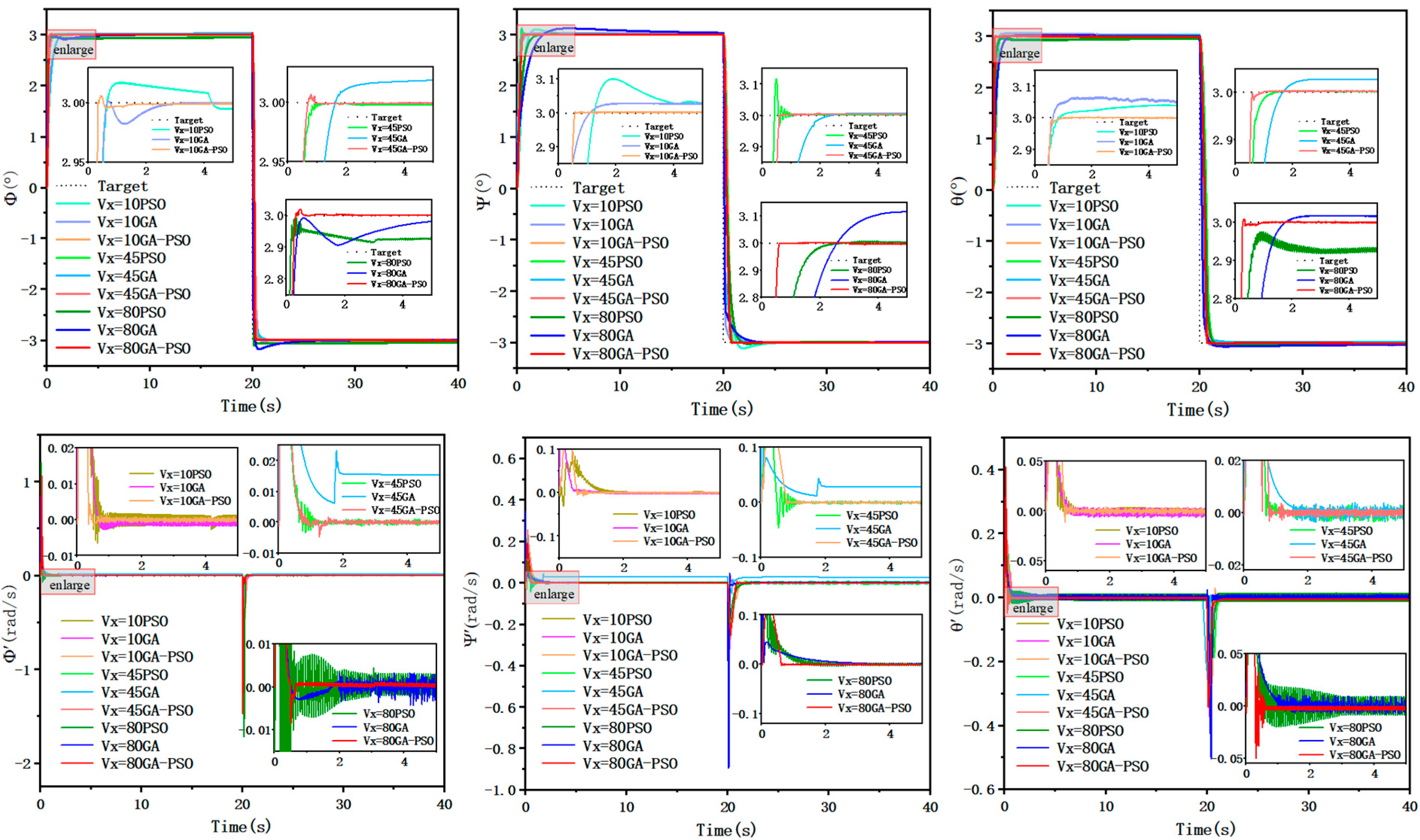
3.2. Verification. of GA-PSO Algorithm

Taking the attitude control loop as an example to verify the GA-PSO algorithm. Table 3 shows the GA-PSO algorithm parameters and their values, which are from the GA or PSO alone. Table 4 shows the ADRC control parameters and corresponding tuned values, which are optimized with the GA-PSO, GA and PSO, respectively. The speeds of 10 m/s, 45 m/s and 80 m/s are selected for the attitude control simulation of different flight modes. The simulation time is 40 s. The 3° step command is given at the beginning of the simulation, and the target attitude is changed to −3° at 20 s. The result is shown in Figure 10. It can be seen that the ADRC with GA-PSO optimized parameters can make attitude response to track target attitude within a short time under different forward speeds. The tracking response is faster and the overshoot, oscillation amplitude of attitude angle and attitude angular rate are smaller than the ADRC with GA or PSO optimized parameters alone. With the increase of forward speed, the former can still maintain a good control effect, while the latter has a worse control effect. The above results show that the ADRC with GA-PSO optimized parameters has the better control effect.

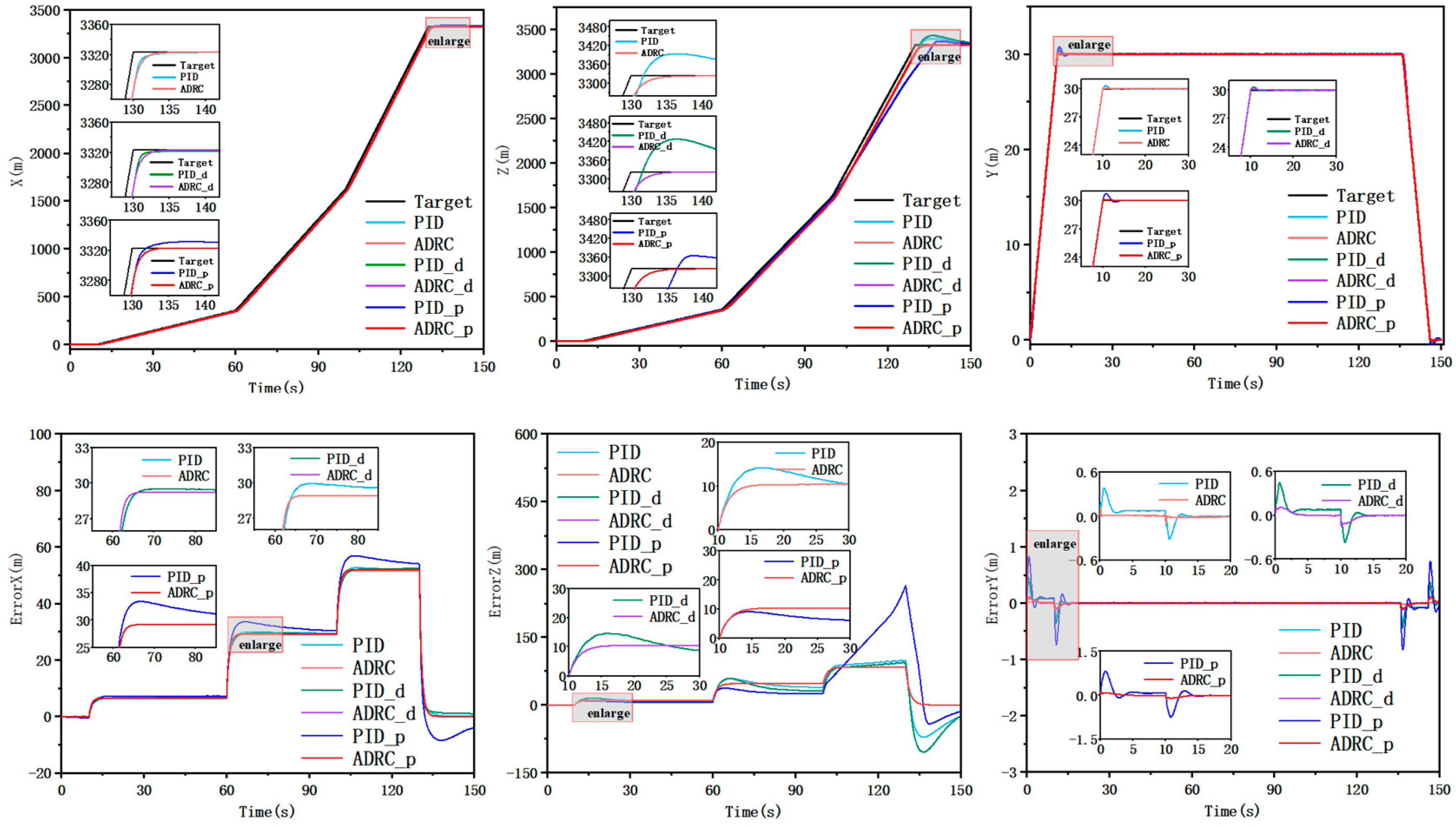
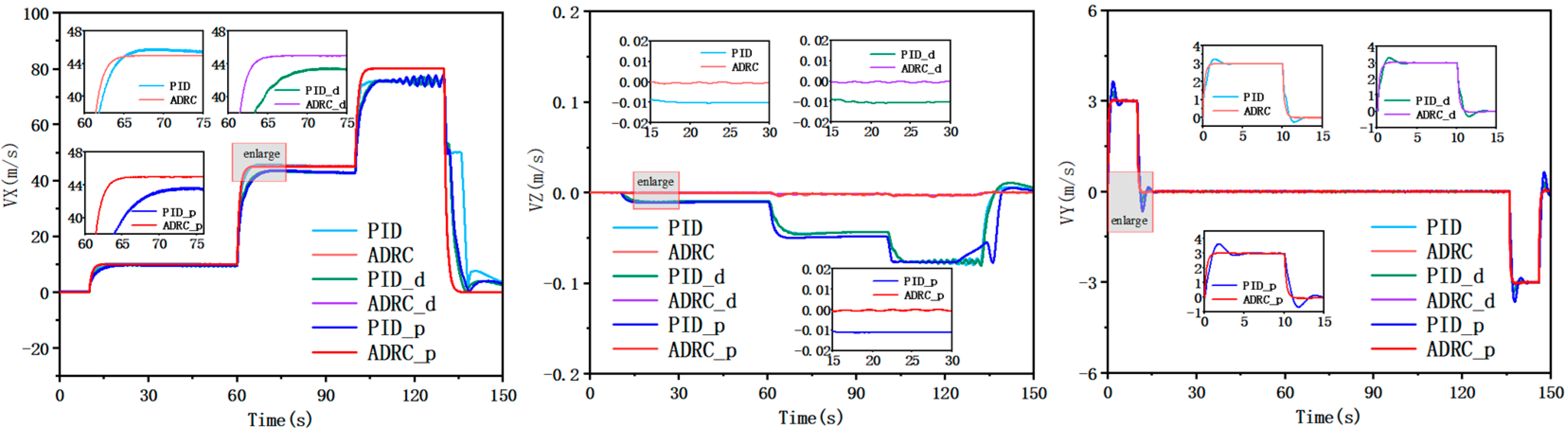
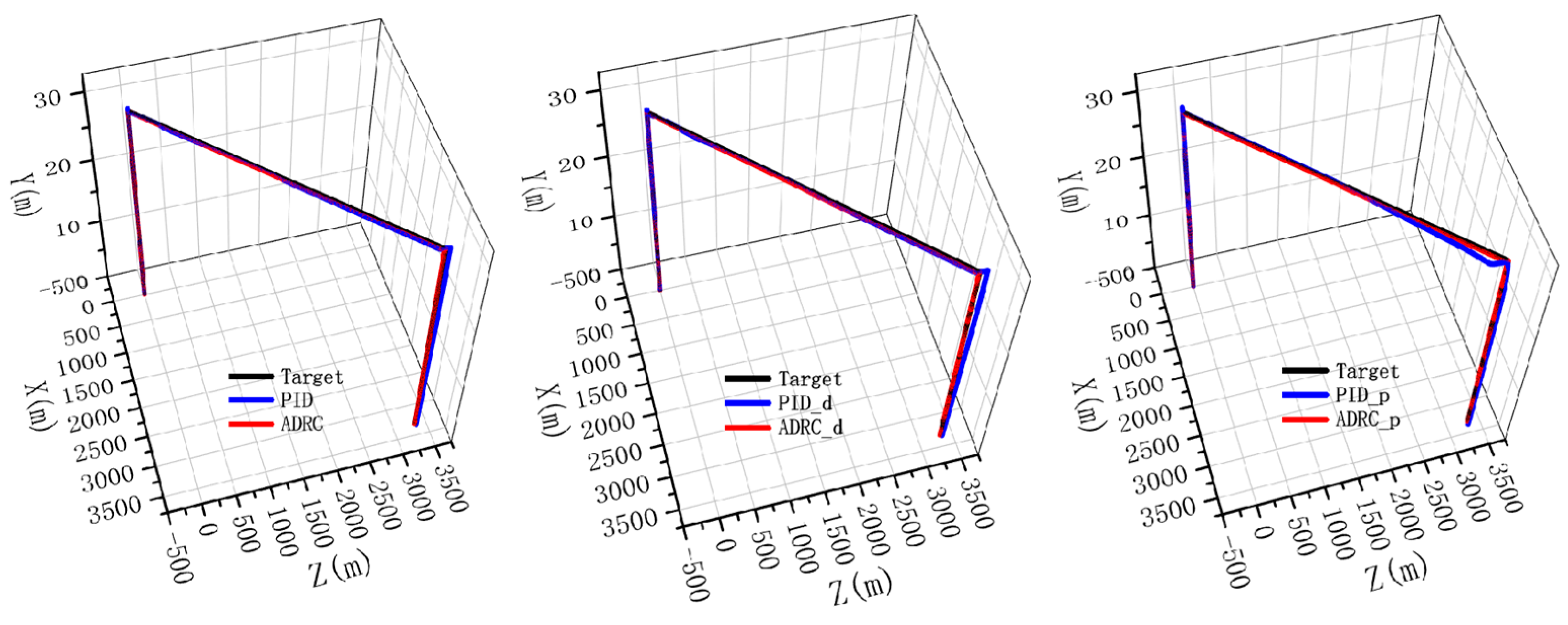
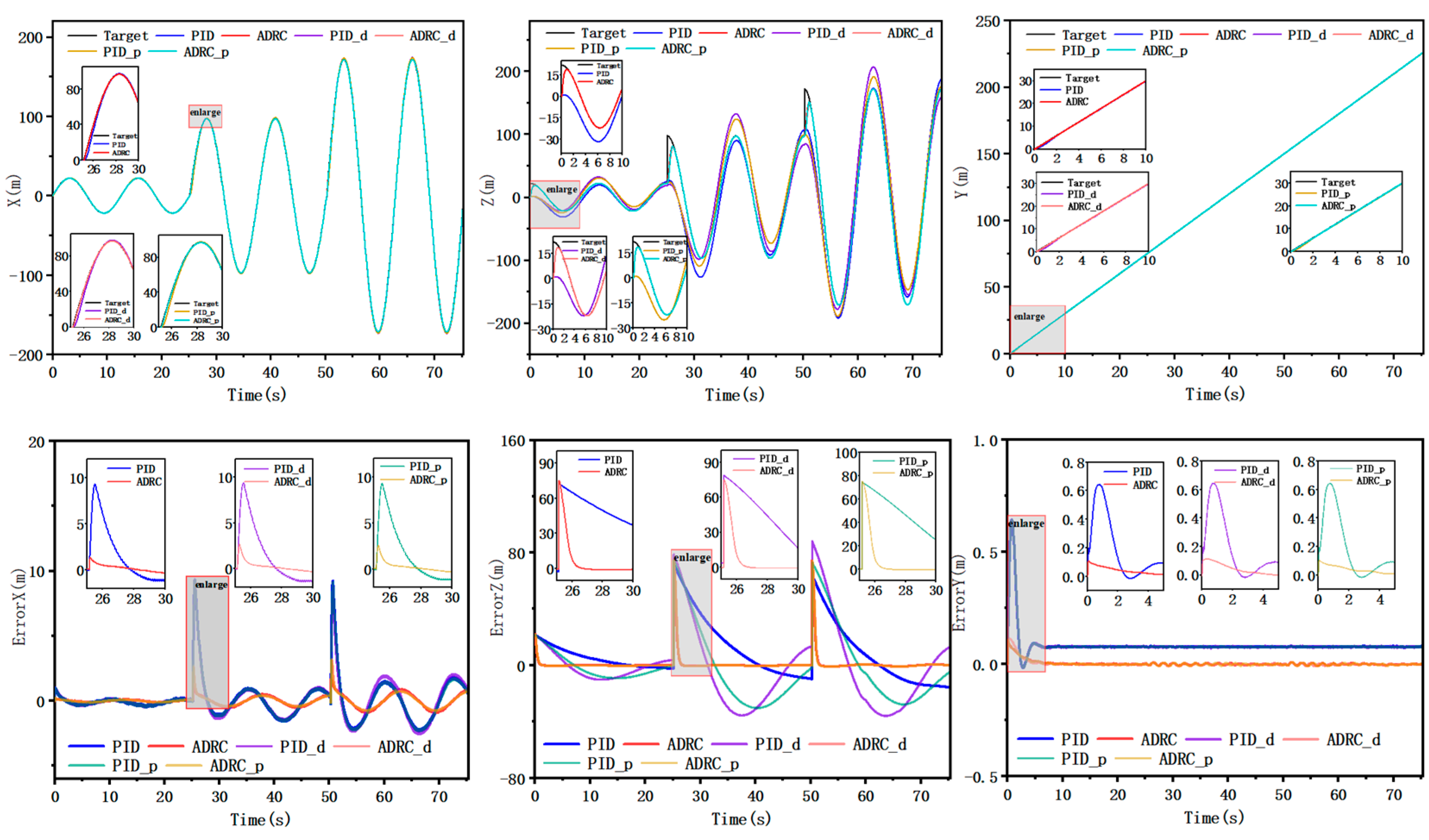
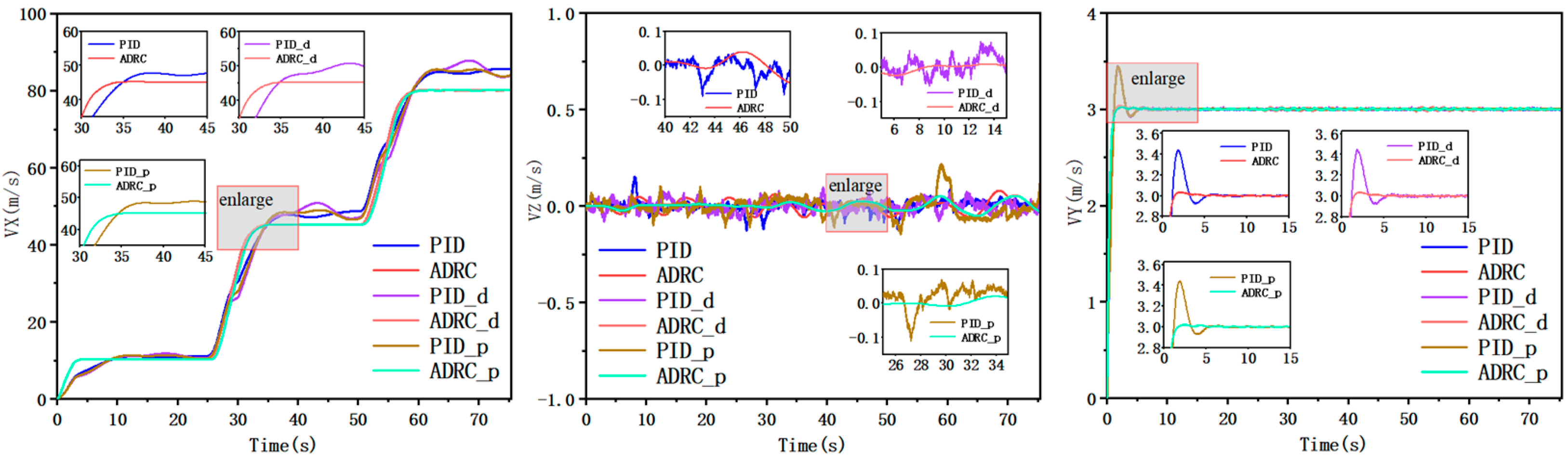
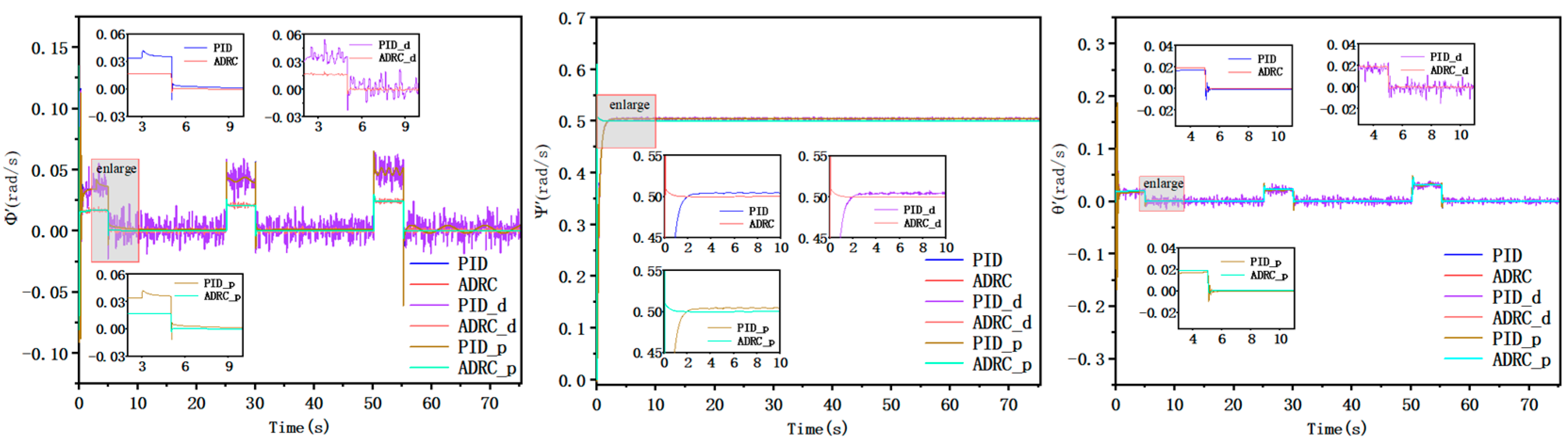
4. Trajectory Tracking Control and Result Analysis

Given the target trajectory, different flight modes and control strategies should be switched according to the forward speed of compound unmanned aircraft. In the simulation, the controller parameters remain unchanged and there are three working situations: no interference signal, measurement signal added with white noise of 10° peak value and the center change of gravity position moved 0.1 m backward (corresponding to PID and ADRC, PID_d and ADRC_d, PID_p and ADRC_p curves in the graphs). The above situations simulate the control effect of ADRC under no interference, external interference and variation of internal parameters, respectively. Then the control effect is compared with that of PID controller. The parameters of PID and ADRC controllers in each channel are shown in Table 5 and Table 6, which are all tuned with GA-PSO algorithm.

4.1. Route Tracking Control with Different Flight Modes

The compound unmanned aircraft takes off vertically at 3 m/s in the first 10 s, then flies forward at 10 m/s in the next 50 s, then flies forward at 45 m/s in the next 40 s, and flies forward at 80 m/s in the next 30 s. In the final 20 s, the UAV reduces the forward flight speed to 0 and lands vertically at 3 m/s. The vertical velocity reduces to 0 during the last 5 s. The trajectory tracking response and velocity response are shown in Figure 11, Figure 12 and Figure 13. The flight modes of the UAV will change with the forward velocity. As the graphs show, even if the forward velocity changes, the ADRC can still maintain fast and stable tracking effect, while the PID control effect becomes worse. The ADRC can still keep a good tracking effect with the external interference or internal parameters changing, especially on the Z axis. The above results show that the ADRC has stronger ability of trajectory tracking, interference rejection and robustness than the PID controller.

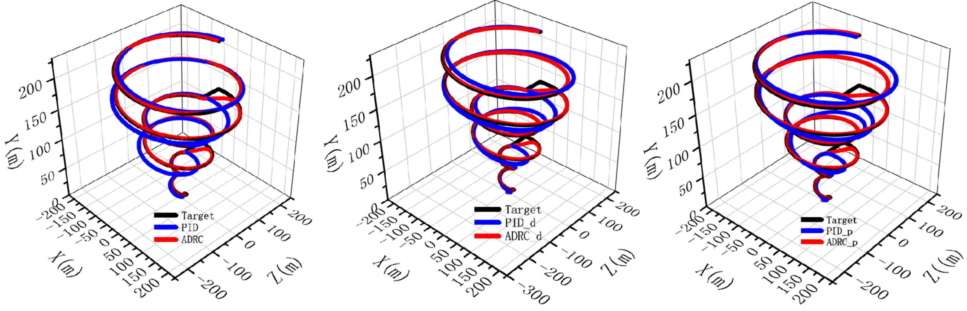
4.2. Climb Tracking Control with Different Flight Modes

The spiral climb tracking control is more complex compared with route tracking control, which can better test the trajectory tracking ability of the compound unmanned aircraft, such as coordinated turning. The climbing velocity of UAV is 3 m/s, and it flies at 10 m/s, 45 m/s and 80 m/s, respectively, in the first 25 s, 25–50 s and the last 25 s. The trajectory tracking response, velocity response and angular rate response are shown in Figure 14, Figure 15, Figure 16 and Figure 17. The flight mode and circulating radius will change with the forward velocity. As the graphs show, even if the forward velocity changes, the ADRC can realize fast and stable tracking of the target trajectory. The tracking velocity and control accuracy are better than those of PID controller, especially on the Z axis. The ADRC can still keep a good tracking effect with external interference or internal parameters changing, while the control effect of PID controller becomes worse. The above results show that the ADRC has higher tracking velocity, stability, interference rejection and robustness than the PID controller.

5. Conclusions

This paper presents a trajectory tracking control system based on ADRC for compound unmanned aircraft. The established nonlinear flight dynamics model and the redundant control strategy can be exploited using the trajectory tracking control simulation in different flight modes. The sigmoid function distributive law can be utilized to transition smoothly between the helicopter mode and airplane mode of the UAV. The designed ADRC can effectively estimate the total disturbance of the controlled plant and be used to compensate the control input. The parameters of the ADRC can be optimized with GA-PSO algorithm. The ADRC with tuned control parameters can ensure the compound unmanned aircraft realizes stable trajectory tracking in full flight mode. Compared with the PID controller, the control effect of ADRC is better for tracking velocity, stability, interference rejection and robustness.

Author Contributions

Writing—original draft preparation, B.D.; writing—review and editing, J.X. All authors have read and agreed to the published version of the manuscript.

Funding

This research was funded by the National Key Laboratory of Rotorcraft Aeromechanics Fund Program of China (9140C400504130C4148) and supported by the Priority Academic Program Development of Jiangsu Higher Education Institutions of China.

Institutional Review Board Statement

Not applicable.

Informed Consent Statement

Not applicable.

Data Availability Statement

Not applicable.

Conflicts of Interest

The authors declare no conflict of interest.

References

  1. Cao, F.; Chen, M. The Utility Model Relates to A Single Rotor Compound Helicopter. J. Beijing Univ. Aeronaut. Astronaut. 2016, 42, 772–779. [Google Scholar] [CrossRef]
  2. Zheng, F.Y.; Liu, L.W.; Cheng, Y.H. Multi-Objective Control Assignment Strategy for Complex Rotorcraft. Acta Aeronaut. Et Astronaut. Sin. 2019, 40, 1–16. [Google Scholar]
  3. Unal, G. Fuzzy robust fault estimation scheme for fault tolerant flight control systems based on unknown input observer. Aircr. Eng. Aerosp. Technol. 2021, 93, 1624–1631. [Google Scholar] [CrossRef]
  4. Topczewski, S.; Narkiewicz, J.; Bibik, P. Helicopter Control During Landing on a Moving Confined Platform. IEEE Access 2020, 8, 107315–107325. [Google Scholar] [CrossRef]
  5. Unal, G. Integrated design of fault-tolerant control for flight control systems using observer and fuzzy logic. Aircr. Eng. Aerosp. Technol. 2021, 93, 723–732. [Google Scholar] [CrossRef]
  6. Kaba, A.; Kıyak, E. Optimizing a Kalman filter with an evolutionary algorithm for nonlinear quadrotor attitude dynamics. J. Comput. Sci. 2020, 39, 1877–1882. [Google Scholar] [CrossRef]
  7. Chaudhary, S.; Kumar, A. Control of Twin Rotor MIMO System Using 1-Degree-of-Freedom PID, 2-Degree-of-Freedom PID and Fractional order PID Controller. In Proceedings of the 2019 3rd International Conference on Electronics, Communication and Aerospace Technology (ICECA), Coimbatore, India, 12–14 June 2019; pp. 746–751. [Google Scholar] [CrossRef]
  8. Gonzalez, H.; Arizmendi, C.; Garcia, J.; Anguo, A.; Herrera, C. Design and Experimental Validation of Adaptive Fuzzy PID Controller for a Three Degrees of Freedom Helicopter. In Proceedings of the 2018 IEEE International Conference on Fuzzy Systems (FUZZ-IEEE), Rio de Janeiro, Brazil, 8–13 July 2018; pp. 1–6. [Google Scholar]
  9. Halbe, O.; Hajek, M. Robust Helicopter Sliding Mode Control for Enhanced Handling and Trajectory Following. In Proceedings of the AIAA SciTech Forum, Orlando, FL, USA, 22 July 2020; pp. 1–23. [Google Scholar] [CrossRef]
  10. Tangm, H.; Yang, H.; Zhou, Y. Trajectory linearization method based on sliding mode observer for unmanned helicopter trajectory tracking control. In Proceedings of the 2018 Chinese Control and Decision Conference (CCDC), Shenyang, China, 9–11 June 2018; pp. 2929–2933. [Google Scholar] [CrossRef]
  11. Ghommam, J.; Saad, M. Autonomous Landing of a Quadrotor on A Moving Platform. IEEE Trans. Aerosp. Electron. Syst. 2017, 53, 1504–1519. [Google Scholar] [CrossRef]
  12. Lu, X.; Zang, X.; Meng, X.; Wang, H. ADRC Based Attitude Control System Design for Unmanned Helicopter. In Proceedings of the 2020 3rd International Conference on Unmanned Systems (ICUS), Harbin, China, 27–28 November 2020; pp. 309–313. [Google Scholar] [CrossRef]
  13. Chen, Y.; Wang, Z.; Lyu, Z.; Li, J.; Yang, Y.; Li, Y. Research on Manipulation Strategy and Flight Test of the Quad Tilt Rotor in Conversion Process. IEEE Access 2021, 9, 40286–40307. [Google Scholar] [CrossRef]
  14. Santos, M.; Juan, M.; Alejandro, J.; Andrés, C. Active Disturbance Rejection Control for UAV Hover using ROS. In Proceedings of the 2018 XX Congreso Mexicano de Robótica (COMRob), Ensenada, Mexico, 12–14 September 2018; pp. 1–5. [Google Scholar] [CrossRef]
  15. Issac, T.; Thomas, F.; Mija, S.J. Trajectory Tracking of Unmanned Helicopter Using Optimized Integral LQR Controller. In Proceedings of the 2020 Fourth International Conference on Inventive Systems and Control (ICISC), Coimbatore, India, 8–10 January 2020; pp. 324–328. [Google Scholar] [CrossRef]
  16. Wu, Z.; Zhou, H.; Guo, B. Review and new theoretical perspectives on active disturbance rejection control for uncertain finite-dimensional and infinite-dimensional systems. Nonlinear Dyn. 2020, 101, 935–959. [Google Scholar] [CrossRef]
  17. Zhou, X.; Zhong, W.; Ma, Y.; Guo, K.; Yin, J.; Wei, C. Control Strategy Research of D-STATCOM Using Active Disturbance Rejection Control Based on Total Disturbance Error Compensation. IEEE Access 2021, 9, 50138–50150. [Google Scholar] [CrossRef]
  18. Zhou, R.; Fu, C.; Tan, W. Implementation of Linear Controllers via Active Disturbance Rejection Control Structure. IEEE Trans. Ind. Electron. 2021, 68, 6217–6226. [Google Scholar] [CrossRef]
  19. Ding, L.; Ma, R.; Wu, H.; Feng, C.; Li, Q. Yaw Control of an Unmanned Aerial Vehicle Helicopter Using Linear Active Disturbance Rejection Control. SAGE J. 2017, 231, 427–435. [Google Scholar] [CrossRef]
  20. Duan, D.; Wang, Z.; Li, J.; Zhang, C.; Wang, Q. Stabilization control for unmanned helicopter-slung load system based on active disturbance rejection control and improved sliding mode control. SAGE J. 2021, 235, 1803–1816. [Google Scholar] [CrossRef]
  21. Dai, J.; Hu, F.; Ying, J. Research on Attitude Control Algorithm Based on Improved Linear Active Disturbance Rejection Control for Unmanned Helicopter. In Proceedings of the 2019 Chinese Control and Decision Conference (CCDC), Nanchang, China, 3–5 June 2019; pp. 1498–1503. [Google Scholar] [CrossRef]
  22. Shen, S.Y.; Xu, J.F. Adaptive Neural Network-Based Active Disturbance Rejection Flight Control of An Unmanned Helicopter. Aerosp. Sci. Technol. 2021, 1, 2–11. [Google Scholar] [CrossRef]
  23. Chen, Z.; Li, Y.; Zhang, Y. Optimization of ADRC Parameters Based on Particle Swarm Optimization Algorithm. In Proceedings of the 2021 IEEE 4th Advanced Information Management, Communicates, Electronic and Automation Control Conference (IMCEC), Chongqing, China, 18–20 June 2021; pp. 1956–1959. [Google Scholar] [CrossRef]
  24. Zhang, D.; Duan, H.; Yang, Y. Active disturbance rejection control for small unmanned helicopters via Levy flight-based pigeon-inspired optimization. Aircr. Eng. Aerosp. Technol. 2017, 89, 946–952. [Google Scholar] [CrossRef] [Green Version]
  25. Huang, Z.; Chen, Z.; Zheng, Y. Optimal Design of Load Frequency Active Disturbance Rejection Control via Double-Chains Quantum Genetic Algorithm. Neural Comput. Applic 2021, 33, 3325–3345. [Google Scholar] [CrossRef]
  26. Shen, S.Y.; Xu, J.F. Trajectory Tracking Active Disturbance Rejection Control of the Unmanned Helicopter and Its Parameters Tuning. IEEE Access 2021, 9, 56773–56785. [Google Scholar] [CrossRef]
  27. Kumar, A.; Ben-Tzvi, P. Estimation of Wind Conditions Utilizing RC Helicopter Dynamics. IEEE/ASME Trans. Mechatron. 2019, 24, 2293–2303. [Google Scholar] [CrossRef]
Figure 1. The compound unmanned aircraft.
Aerospace 09 00313 g001
Figure 2. Weight coefficient distribution.
Aerospace 09 00313 g002
Figure 3. Structure of ADRC.
Aerospace 09 00313 g003
Figure 4. Trajectory tracking control structure.
Aerospace 09 00313 g004
Figure 5. Attitude controller.
Aerospace 09 00313 g005
Figure 6. Velocity controller.
Aerospace 09 00313 g006
Figure 7. Position controller.
Aerospace 09 00313 g007
Figure 8. GA-PSO algorithm combined with ADRC control system.
Aerospace 09 00313 g008
Figure 9. GA-PSO flow chart.
Aerospace 09 00313 g009
Figure 10. Attitude response with different forward speeds.
Aerospace 09 00313 g010
Figure 11. Three-axis trajectory tracking response and error.
Aerospace 09 00313 g011
Figure 12. Three-axis velocity response in body axis.
Aerospace 09 00313 g012
Figure 13. 3D trajectory response.
Aerospace 09 00313 g013
Figure 14. Three-axis trajectory tracking response and error.
Aerospace 09 00313 g014
Figure 15. Three-axis velocity response in body axis.
Aerospace 09 00313 g015
Figure 16. Roll, yaw, pitch angular rate response.
Aerospace 09 00313 g016
Figure 17. Spiral climb 3D trajectory response.
Aerospace 09 00313 g017
Table 1. Main parameters of the UAV.
NameParameterNameParameter
Take-off weight20 kgRotor radius0.72 m
Rotor speed1600 r/minPropeller radius0.16 m
Num of rotor blades2Num of Propeller blades3
Table 2. Control strategies for different flight modes.
Control ChannelHelicopterTransitionAirplane
Yaw attitudepropeller speedpropeller speedpropeller speed
Roll attitudelateral pitchlateral pitch, aileronaileron
Pitch attitudelongitudinal pitchlongitudinal pitch, elevatorelevator
Forward velocitylongitudinal pitchlongitudinal pitch, propeller speedpropeller speed
Vertical velocitycollective
pitch
elevator, collective pitchelevator, collective pitch
Table 3. Algorithm Parameters of GA-PSO.
ParameterDescriptionGA-PSO
NGEvolution number of GA100
sizepopPopulation size of GA80
swarmsizeParticles number80
DParameters tuning number30
c1Speed factor1.49
c2Speed factor1.49
Table 4. Control Parameters optimized with GA-PSO, GA and PSO.
Controllerrh [β1, β2]τδ [β01, β02, β03]b
ΦGA-PSO2.20.92 [2500, 10]5545.3 [65, 3500, 2.9]6.5
ΨGA-PSO22 [9500, 0.5]350.005 [3, 20, 0.1]0.05
θGA-PSO23 [11.28, 30]5.80.6 [9, 20.5, 0.5]8.8
ΦGA50.92 [5000, 10]3030 [19.65, 1082, 11]1
ΨGA22 [9500, 0.5]35.30.01 [3, 20, 0.1]0.05
θGA51 [139, 22]26.9300 [9, 20.5, 0.1]8.8
ΦPSO2.20.9 [6000, 15]5245 [55, 3300, 2.9]3.5
ΨPSO22 [9500, 0.5]350.005 [3, 20, 0.1]0.05
θPSO23 [10.5, 30]5.21 [8, 18.5, 0.8]5.5
Table 5. Parameters of PID controller.
Controller Ψ . Φ . θ . ΨΦθVxVyVzXYZ
kp1500150155002005.220001005001203055
ki10300000.350301250.01121.1
kd1001500000115305100
Table 6. Parameters of ADRC.
Controllerrh [β1, β2]τδ [β01, β02, β03]b
Φ205 [3000, 100]8020 [31, 5000, 50]15
Ψ3001.2 [60, 20,000]100010 [80, 20,000, 20,000]80
θ5150 [500, 50]155 [15, 120, 100]0.1
Vx51 [1000, 100]50080 [180, 150, 5]0.2
Vy5150 [500, 20]300.5 [20, 200, 50]0.1
Vz3010 [1500, 200]801 [2, 163, 15]6
X102 [1200, 80]10005 [35, 120, 5]20
Y205 [50, 10]2002 [10, 60, 100]0.5
Z3015 [12.5, 72]165100 [12, 3500, 100]26
Publisher’s Note: MDPI stays neutral with regard to jurisdictional claims in published maps and institutional affiliations.

