Article

Probability Analysis of Widespread Fatigue Damage in LY12-CZ Aluminum Alloy Single-Row Seven-Hole Plate

1
College of Aerospace Engineering, Nanjing University of Aeronautics and Astronautics, Nanjing 210016, China
2
China Special Vehicle Research Institute, Jingmen 448000, China
3
Jinling Institute of Technology, College of Mechanical and Electrical Engineering, Nanjing 211169, China
4
AVIC Chengdu Aircraft Industral (Group) Co., Ltd., Chengdu 610092, China
5
AVIC Jincheng Nanjing Engineering Institute of Aircraft System, Nanjing 211106, China
6
Shanghai Electro-Mechanical Engineering Institute, Shanghai 201109, China
*
Author to whom correspondence should be addressed.
Aerospace 2022, 9(4), 215; https://doi.org/10.3390/aerospace9040215
Submission received: 12 March 2022 / Revised: 4 April 2022 / Accepted: 11 April 2022 / Published: 14 April 2022
(This article belongs to the Section Aeronautics)

Abstract

:
In order to determine the average behavior time of widespread fatigue damage (WFD) in an aircraft multi-site damage (MSD) structure and complete the fatigue analysis of WFD sensitive parts, this paper adopts a probabilistic method to analyze the crack initiation and crack propagation of a single row of collinear seven-hole plates. The simulation analysis of the whole process from crack initiation to structural failure is realized. First, through statistical analysis of the test data of the LY12-CZ alloy single-detail plate with hole, the probability distribution of crack initiation life and growth rate is obtained, and this probability distribution is expressed by the randomization of variables. Then, using the related theories of fracture mechanics and fatigue statistics, the whole process of initiation, propagation, and connection of multiple cracks in the MSD structure to the occurrence of WFD was realized through the Monte Carlo method. Finally, a group of single-row seven-hole plate examples are used to verify the accuracy of the calculation results. The results show that the calculated results in this paper are in good agreement with the experimental data, and can accurately predict the life of MSD structures under a certain reliability.

1. Introduction

Widespread fatigue damage (WFD) refers to the simultaneous occurrence of cracks with sufficient size and density in multiple detailed parts of the structure, so that the structure cannot meet the residual strength requirements [1]. In April 2006, the FAA published the “Aging Aircraft Plan: Widespread Fatigue Damage, Revised Draft”, requiring analysis of safety factors before widespread fatigue damage occurs, and requiring WFD assessment related to initial operational limits for existing aircraft and aircraft under review [2]. The key to the widespread fatigue damage assessment is to determine the average time of WFD behavior.
Since the Aloha accident in 1988, researchers at home and abroad have carried out a great deal of research on WFD and multi-site damage (MSD). A series of achievements have been made in multi-crack initiation and mechanisms, calculation methods of the stress intensity factor, crack propagation and connectivity, residual strength, probability assessment methods, and so on. On the basis of deterministic analysis theory, using the method of probability and statistical analysis to solve the problem and obtain the fatigue life under a certain reliability is the research direction of WFD. In this paper, fracture mechanics and fatigue statistics are combined, and then the randomness of the process of initial crack initiation and crack propagation is simulated with the help of finite element analysis software and the Monte Carlo method, so as to realize the random initiation and propagation of multiple cracks and simulate the occurrence process of widespread fatigue damage.
For the crack initiation of an MSD structure, it is generally considered that the cracks do not affect each other. The crack initiation life of an MSD structure is predicted by comprehensively analyzing the geometric characteristics, material parameters, and test data of the structure. For determining the initial crack initiation position and sequence, there are mainly three random crack initiation methods: the random crack initiation method based on the fatigue test results of a single-detail structure, the random crack initiation method based on the material S-N curve, and the random crack initiation method based on the equivalent initial defect size (EIFS). According to the crack initiation life of a single-detail structure, Xi [3] established the probability calculation model of multi-detail crack initiation life, which was verified by experiments. Considering the dispersion of materials, Yan [4] used the Monte Carlo method to analyze the probability of widespread fatigue damage of a five-hole plate. Ai [5] proposed a probabilistic model to illustrate the impact of manufacturing defects on fatigue life based on the size and location of defects. Kim et al. [6] considered the uncertain factors such as initial defects, material variability, and crack growth rate, and combined the Gaussian process response model with the propagation finite method to obtain the response surface and sensitivity factors of multiple crack propagation in the structure under a complex environment, so as to consider the randomness of crack initiation.
For MSD structures, the interaction between multiple cracks will affect the crack growth rate. When the crack grows to a certain size, the influence between cracks intensifies, and the crack interference leads to a sharp increase in the crack growth rate. Wang et al. [7] proved that MSD crack interference would accelerate crack propagation in long crack propagation through fatigue tests and numerical analysis on a three-row plate with holes. At present, many scholars have carried out a great deal of research on the random process of WFD crack propagation. Ray A. [8] randomly modeled the Paris formula based on the fatigue model of probabilistic fracture mechanics. In this method, the material parameter C in the Paris formula is regarded as a random variable to simulate the randomness of crack propagation, which makes the model have a simpler mathematical form and more truly reflect the dispersion of structural crack propagation. H. Riahi, Ph. Bressolette, etc. [9]. proposed a new random configuration method to solve the problem of mixed-mode fatigue crack growth with random parameters. This method has higher numerical calculation efficiency. The response surface method (RSM) and the direct coupling method (DCM) were used by Edson et al. [10] to solve the random crack propagation problem. The boundary element method (BEM) was used to simulate the crack propagation effectively and avoid the re-meshing. At present, Monte Carlo simulation is often used to simulate the random fatigue crack growth. Salimi et al. [11] simulated the uncertainty of crack growth model parameters by the Monte Carlo simulation method, and analyzed the random crack growth.
The stress intensity factors of multi-crack and single-crack structures are quite different. Because the multi-crack structure is affected by the interaction between cracks, the stress intensity factor will change under the interaction of cracks. In addition, crack connectivity will have a great impact on the stress intensity factor. For the problem of multiple cracks around the hole, the randomness of crack distribution increases the complexity of solving the stress intensity factor. In engineering, the finite element method is more used to calculate the stress intensity factor of multiple cracks. Atluri et al. [12] proposed the finite element alternating method (FEAM) and elastic–plastic finite element alternating method (EPFEAM) in solving stress intensity factors. The two methods can save the time of redrawing the mesh and reconstructing the stiffness matrix, and ensure the calculation accuracy. Wu L. et al. [13] studied the calculation of the stress intensity factor of multiple cracks near collinear holes, and developed a set of semi-analytical numerical calculation methods.
At present, a variety of strength criteria and models have been developed for the study of residual strength. The core problem in MSD is to study the residual strength of the structure. The connection between cracks is a special failure phenomenon in an MSD structure. When two adjacent collinear cracks expand to a certain extent, they will be connected with each other. Swift et al. [14] proposed and applied a new ligament yield criterion in the plastic zone when studying the crack connectivity criterion, and found that the result was accurate by comparing it with the test results. Later, Chinese scholars Ge S. and Li Z. [15] used the swift failure criterion to study the residual strength of butt skin connection. The results show that the accuracy of the calculation results of the swift connection criterion deviates, so the swift criterion needs to be corrected. Bert et al. [16] modified the crack connectivity model through tests, and the modified crack connectivity model has a wider area of application. Wang et al. [17] tested an MSD structural aluminum plate and verified five failure criteria. The results show that there is a large difference between the net section criterion and CTOA criterion; the plastic zone connectivity criterion and average displacement criterion are more accurate, and the fracture mechanics criterion is more suitable for the case of obvious main cracks.
In this paper, the fatigue crack propagation test of a single-row collinear seven-hole plate structure is carried out. The probability method is used to analyze the crack initiation and propagation at the hole edge of a single row of seven-hole plates, and the simulation analysis of the whole process from crack initiation to structural failure is realized. In order to calculate the stress intensity factor at the crack tip, the singularity setting and meshing of the crack are carried out by ABAQUS, and the stress intensity factor with high accuracy is obtained. Finally, the average WFD behavior is calculated by the Monte Carlo sampling method.

2. Fatigue Test of Single-Detail Perforated Plate

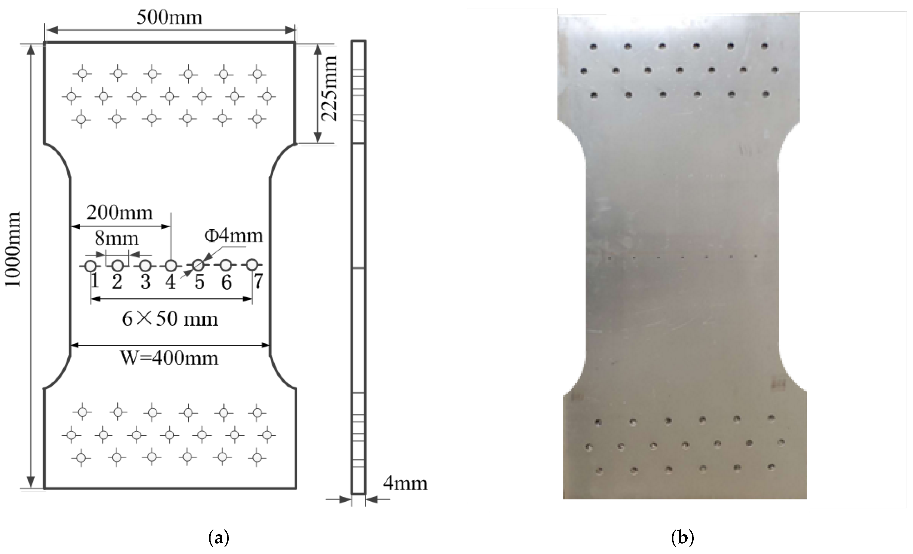
2.1. Test Piece Preparation
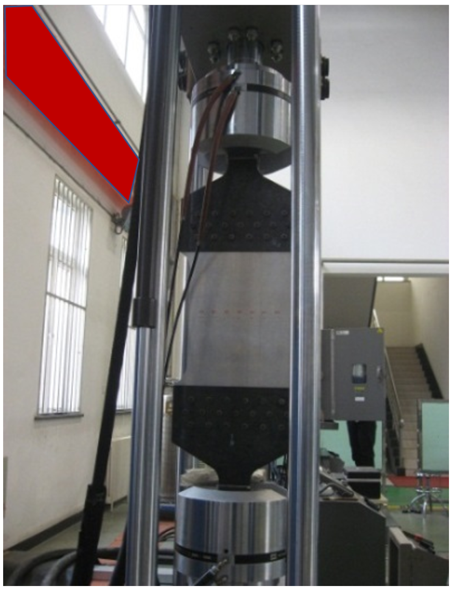
In order to study the crack initiation life probability distribution and crack propagation rate of the LY12-CZ aluminum alloy perforated plate with pre-crack, a single-detail plate test piece with a hole was prepared. We made a circular hole with a diameter of 3 mm in the center of the test piece, pre-made cuts with a length of 3.5 mm on the left and right sides of the circular hole, and took the sum of the radius of the hole and the length of the crack on the side of the hole as the half-crack length. The size of the test piece is shown in Figure 1. LY12-CZ aluminum alloy was used as the material, and the material parameters are listed in Table 1. In the table, E is the Young’s modulus, μ is Poisson’s ratio, K C is fracture toughness, and σ s is the yield strength.

2.2. Test Procedure

The specimens were mounted on a 100 kN MTS fatigue/static testing machine for the fatigue test, and the cracks were measured with a manual reading microscope. When a 0.5 mm crack was generated on the basis of the prefabricated crack, i.e., the half crack length was 5.5 mm, the number of cycles at this time was recorded as the crack initiation life. After this, the crack growth rate test was continued, and the crack length and cycle number ( a i N i ) of the test piece were recorded every 5000 cycles until the test piece was broken. The test piece planning and load spectrum are shown in Table 2.
A total of 15 fatigue tests were completed. Figure 2a shows the crack initiation life point and S N i n i t curve. Figure 2b–d are the crack growth curves at 15.20 kN, 18.24 kN, and 19.76 kN stress levels, respectively. It can be seen that the crack initiation and propagation between different test pieces have a certain degree of dispersion.

3. Random Crack Initiation Model of MSD Structure

For an MSD structure, it is assumed that there are T details (as shown in Figure 3), which may initiate collinear cracks. Because of the dispersion of crack initiation, the location of crack initiation is random [18].
The most commonly used form to describe the S-N curve of materials is the power function, which is
S m N = C
and among them, m and C are parameters related to the material, stress ratio, and loading mode. For the crack initiation life curve at position i of the MSD structure, it can be expressed by the following equation:
S m N i n i t i = C i
where N i n i t i is crack initiation life at position i, and C i is a random variable used to simulate the dispersion of crack initiation life. In fatigue statistics [19], it is generally believed that the lognormal distribution can be used to describe the distribution of life N. Since the crack initiation life accounts for a large part of the entire fatigue life, it is believed that the crack initiation life also obeys the lognormal distribution.
Under the same stress level, S m in Equation (2) is a constant. Therefore, in order to ensure that N i n i t i obeys lognormal distribution, we only need to make the logarithm of C i obey normal distribution, i.e.,
log C i = log C i ¯ + S log C i C 0 i
In the formula, log C i ¯ is the logarithm mean of C i , S log C i is the logarithmic standard deviation of C i , and C 0 i is a random variable, which obeys the standard normal distribution. By Equation (2), we have
log C i ¯ = log N i n i t i ¯ + m log S
Since m log S is a constant, we obtain that
S log C i = S log N i n i t i
where log N i n i t i ¯ is the logarithmic mean value of crack initiation life N i n i t and S log N i n i t i is the logarithmic standard deviation of crack initiation life N i n i t .
By substituting Equations (4) and (5) into Equation (3), C i can be obtained. Then, substituting C i into Equation (2), the crack initiation life N i n i t i at different positions i ( i = 1 , 2 , , T ) under the MSD structure can be obtained. By sorting the crack initiation life at different positions i, the order of crack initiation and the crack initiation life at each position in the MSD structure can be obtained. The smallest crack initiation life is the crack initiation life of the structure N m i n .
N m i n = m i n { N i n i t i , N i n i t i , , N i n i t T }
log N i n i t i ¯ is obtained by statistical analysis of crack initiation life in Figure 2. Then, the values of log C i and S log C i are obtained by Equations (4) and (5), as shown in Table 3.

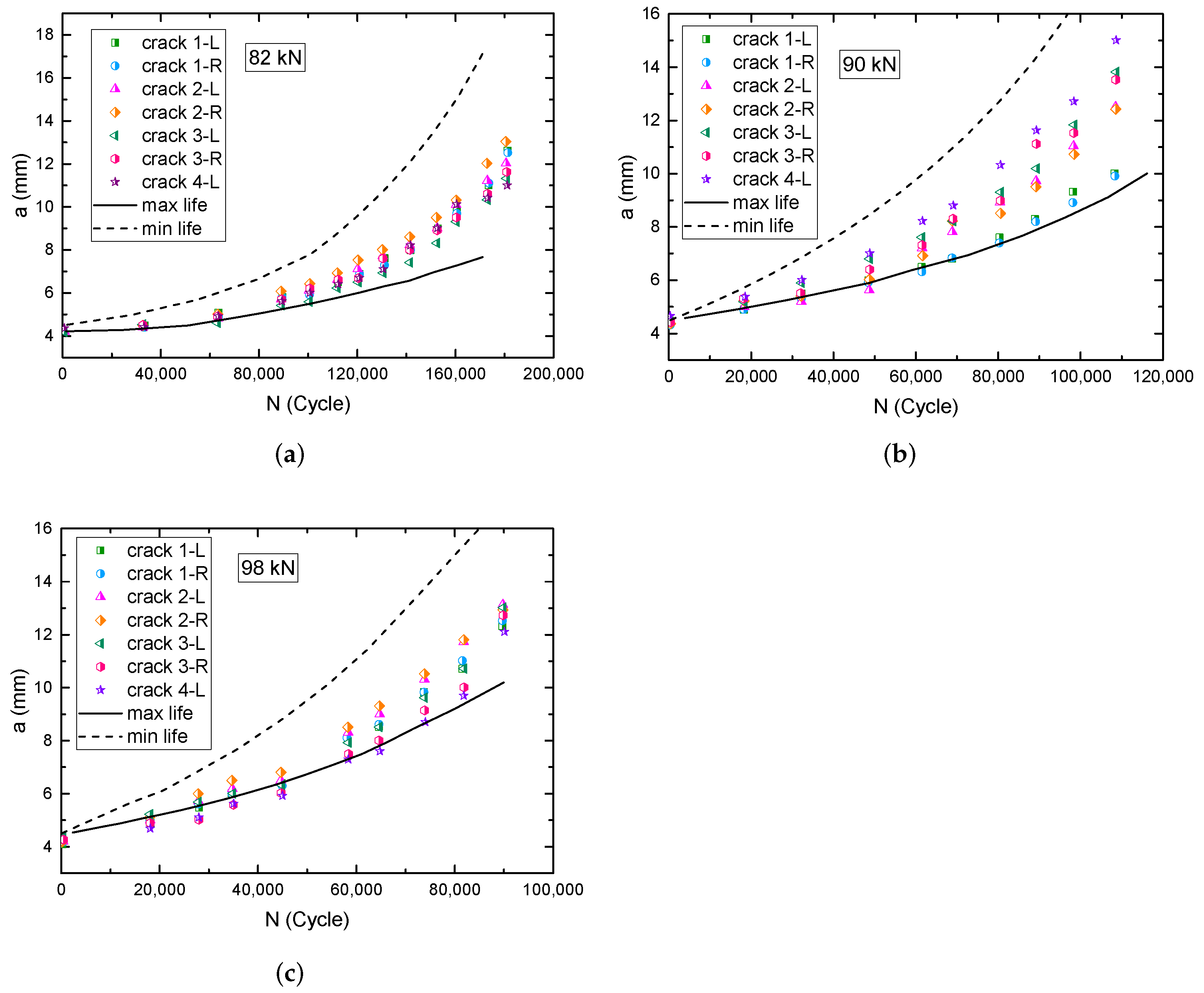
4. Random Crack Propagation in MSD Structure

4.1. Crack Propagation Model Based on Random Variables

The crack growth rate ( d a / d N ) of fatigue cracks has a certain relationship with the magnitude of the stress intensity factor ( Δ K ). Paris [20] proposed the famous Paris formula in 1963 to describe the relationship between d a / d N and Δ K :
d a / d N = D ( Δ K ) n
The above formula points out that the stress intensity factor amplitude Δ K is the main control parameter of the fatigue crack growth rate d a / d N . When Δ K increases, the crack growth rate d a / d N increases. D and n are the basic parameters describing the fatigue crack growth performance, which are determined by tests.
In order to describe the dispersion of crack growth, D and n are used to randomize into D i and n i ( i = 1 , 2 , , T ) by using the method of random variables, and Equation (7) is expressed in logarithmic form, i.e.,
log ( d a / d N ) = log D i + n i log ( Δ K )
The three-parameter lognormal distribution can better represent the variability of random parameters [4]. The variable u i is introduced, namely
u i = D i ¯ D i
where D i ¯ is the mean value of the random parameter D i , obtained by tests.
Therefore, the probability density function of u i satisfies the three-parameter lognormal distribution, as follows [18]:
f ( u i ) = 0.43429 ( u i τ ) 2 π β e x p 1 2 log ( u i τ ) α β 2
In the formula, τ is the position parameter, α is the dispersion parameter, and β is the shape parameter. According to the properties of the three-parameter normal distribution, the following formula can be obtained.
log ( u i τ ) = α + β D 0 i
where D 0 i is a random number that obeys the standard normal distribution, which is generated by a random generator. Substituting Formula (9) into (11) can obtain the value of D i :
D i = D i ¯ 10 α + β D 0 i + τ
Because there is a strong linear relationship [21] between log D i and n i , the two parameters were analyzed by linear regression.
log D i = l 0 × n i + l 1
The value of n i can be obtained.
n i = log D i l 1 l 0
where l 0 and l 1 are regression parameters.
Finally, after the random crack growth parameters are obtained by Equations (12) and (14), the crack growth rate d a / d N can be obtained by Equation (8).

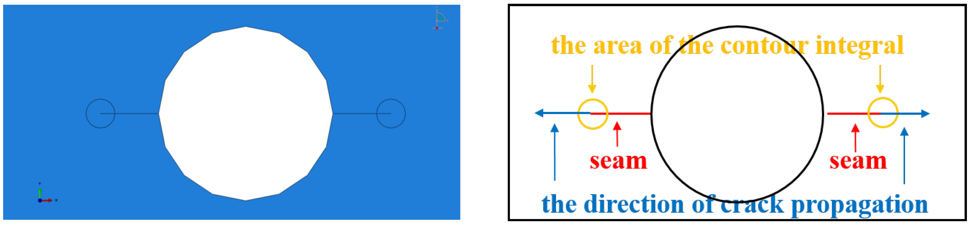
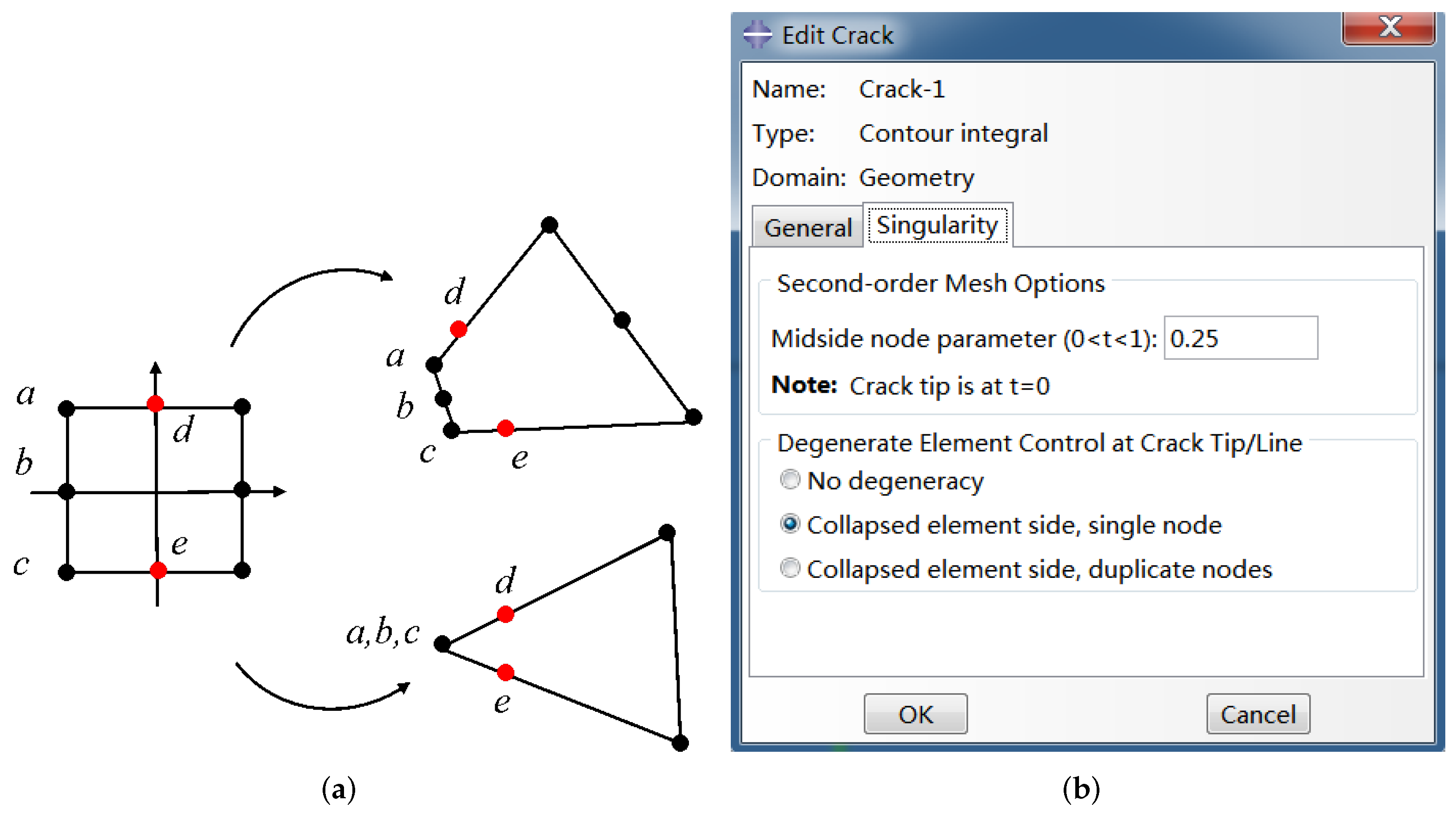
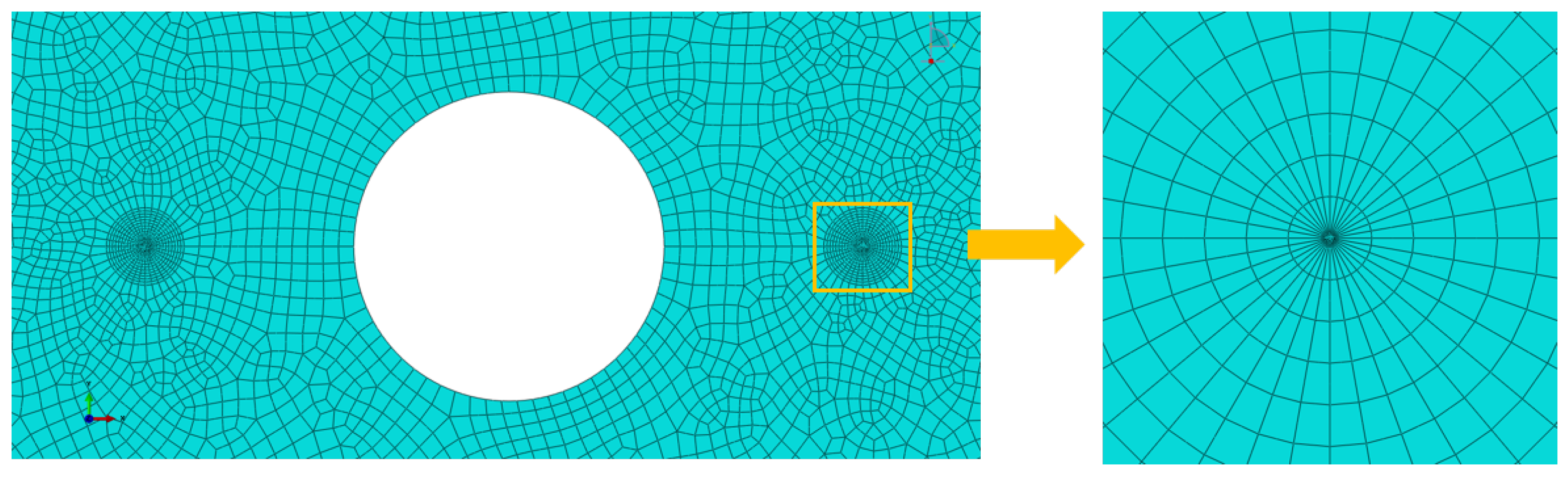
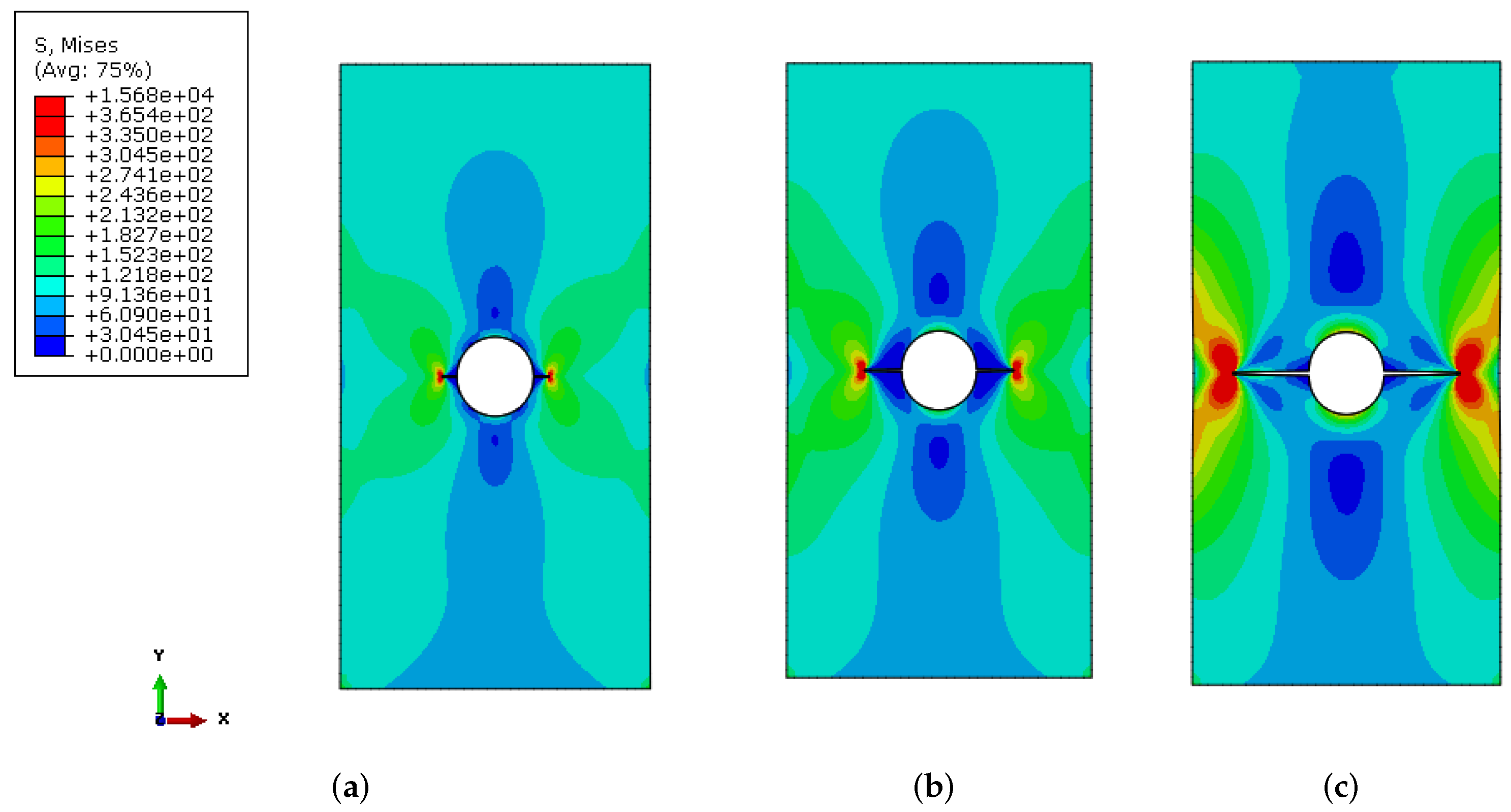
4.2. Calculation of Stress Intensity Factor by FEM

The accuracy of solving the stress intensity factor is related to the accuracy of crack propagation analysis and calculation. In this paper, the stress intensity factor is calculated by ABAQUS software. Its essence is to calculate the stress intensity factor by the finite element method (FEM). Since the stress intensity factor needs to be calculated continuously in the process of crack propagation, ABAQUS CAE is redeveloped in this paper to improve the calculation efficiency.
For the finite element model with cracks around the hole, it is necessary to focus on the definition of cracks and the division of the mesh at the crack tip. In ABAQUS, defining a crack requires two steps: 1. the line segment as the crack is first defined as the “seam”, and the meshes on both sides of the line segment defined as the “seam” will be separated to simulate the cracking of the crack during calculation; 2. we determine the area of the contour integral and the direction of crack propagation by creating a “crack” (as shown in Figure 4).
Due to the stress concentration phenomenon of the crack tip with a large geometric deformation gradient, it is necessary to define a circle of 1/4 singularity elements surrounding the crack tip, and collapse the crack tip location element node into a node, which is used to approximate the crack tip location with singularity. In ABAQUS, there are special options for crack editing to set the singularity of the crack tip. Generally, the grid element of the crack tip is specified as an eight-node quadrilateral element, and the node is offset by 1/4 to simulate the singularity of the crack tip.
Figure 5 shows the schematic diagram of singularity grid node offset and relevant settings in ABAQUS. In Figure 5a, nodes a, b, and c are close to the crack tip, so the three nodess will collapse into one node. It is necessary to set the option “collapsed element side, single node” in the ABAQUS singularity setting dialog box. At the same time, in order to describe the singularity of the crack tip, points d and e are offset 1/4 toward the crack tip.
As the model is a flat plate structure with holes and cracks at the edge of the hole, the meshing of different areas is different. The crack tip area is taken as the key assessment area, and the quality of meshing determines the accuracy of solving the stress intensity factor. It is necessary to densify the mesh and adopt the sweeping mesh generation technology in the contour area of the crack tip. We then divide other areas into a structured mesh. The element type is CPS8. The meshing of the crack tip is shown in Figure 6.
In order to prove the accuracy of the finite element method to calculate the stress intensity factor, the single-hole plate shown in Figure 7 was analyzed, and the calculated stress intensity factor results were compared with the Handbook of Stress Intensity Factor. The tensile stress of the single-hole plate in the vertical direction is 100 MPa, and the crack length a is 2 mm, 5 mm, and 10 mm, respectively.
Figure 8 shows the stress distribution of the single-hole plate with a value of 2 mm, 5 mm, and 10 mm, respectively. As the crack length increases, the net cross-section area of the plane where the crack is located gradually decreases, resulting in an increasing stress concentration at the crack tip. Table 4 shows the comparison between the value of the stress intensity factor calculated by FEM described in this paper and obtained by querying the Handbook of Stress Intensity Factor. The results show that the value of the stress intensity factor calculated by FEM is approximately 1% different from that in the Handbook of Stress Intensity Factor, indicating that the stress intensity factor calculated by FEM in this section has high accuracy.
The above analysis shows that the ABAQUS method described in this section has high accuracy in calculating stress intensity factors.

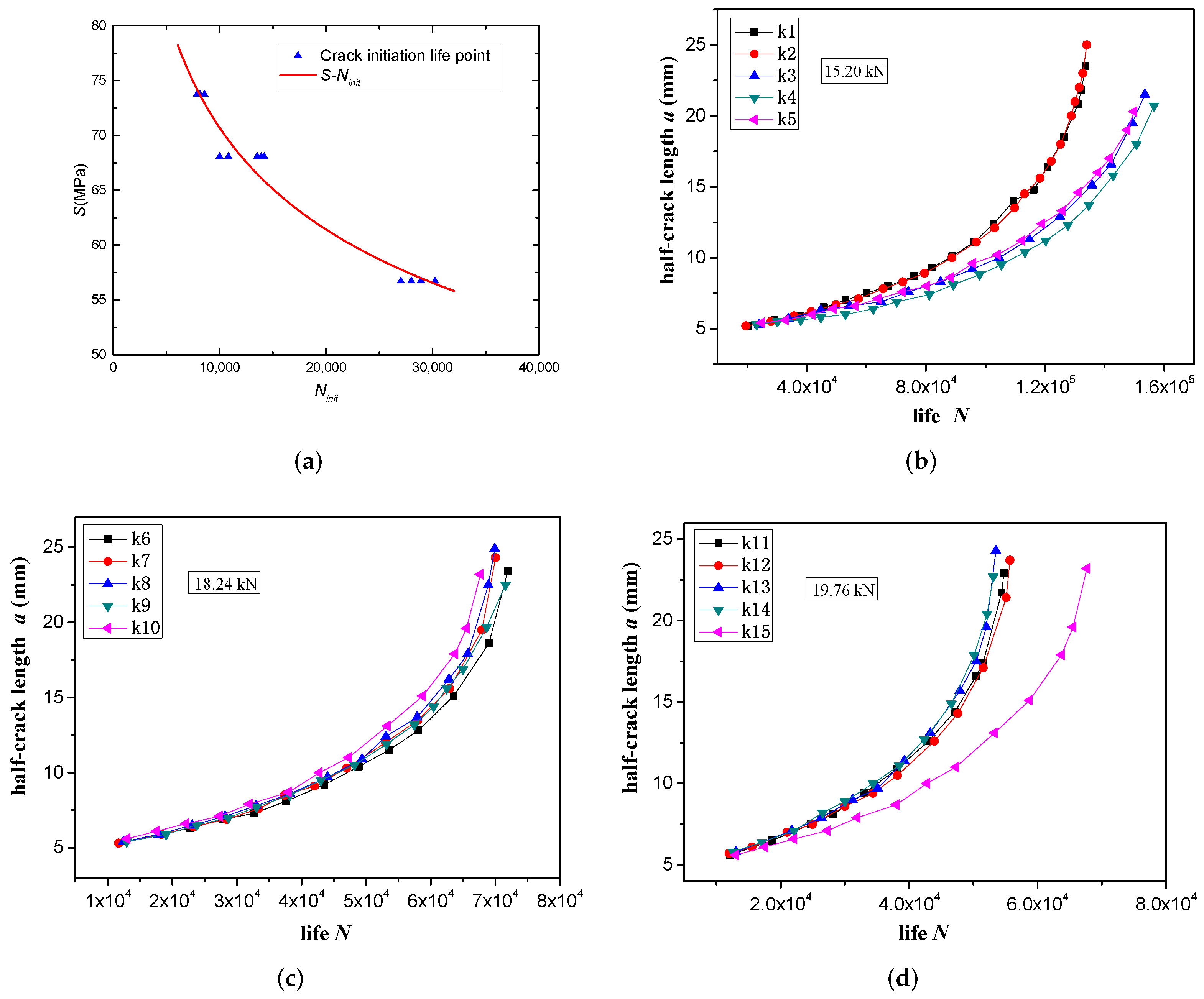
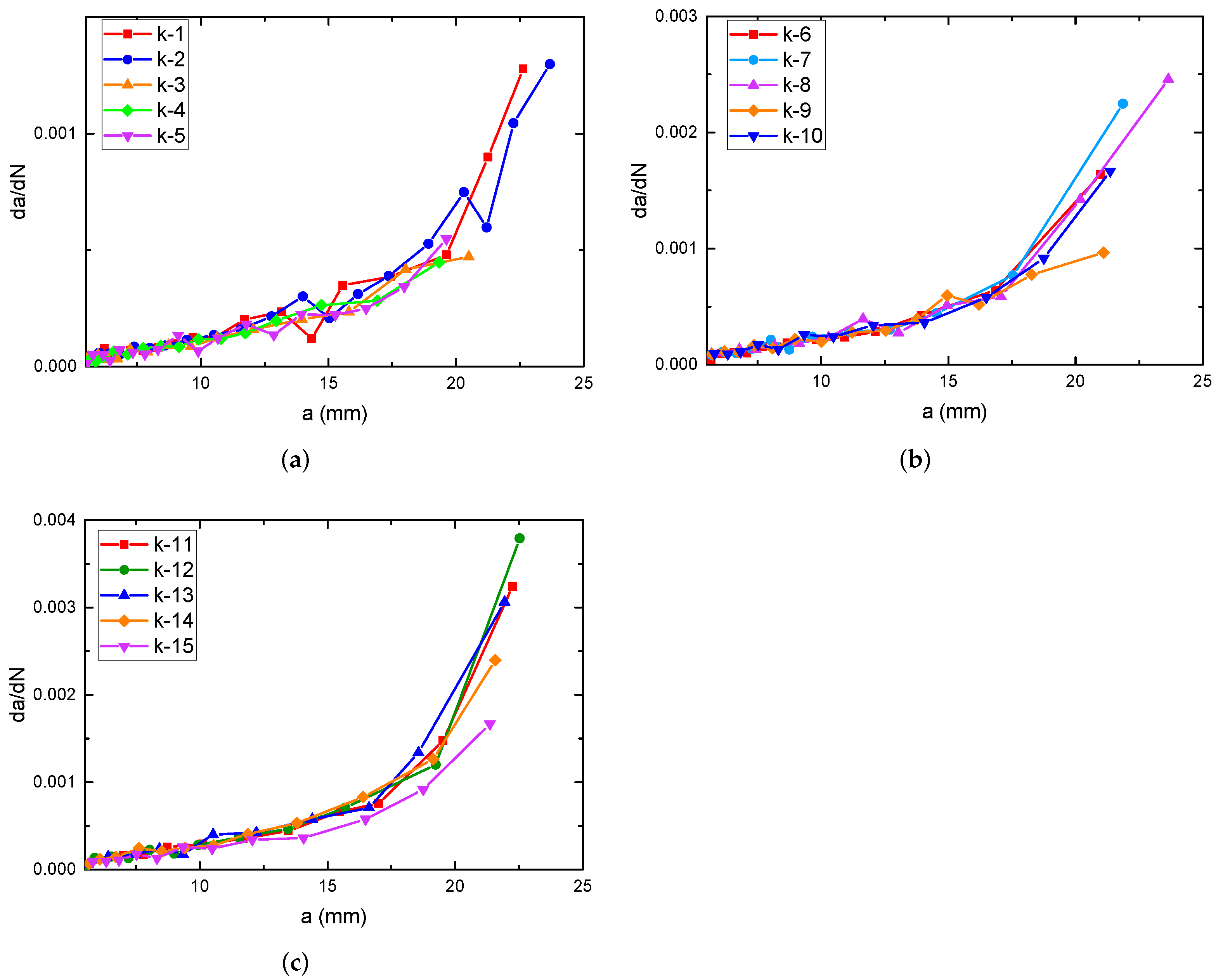
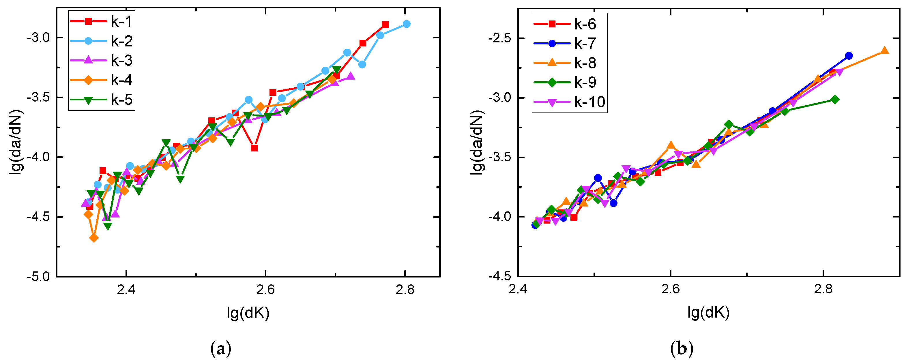
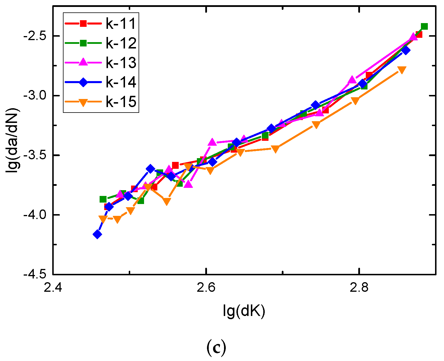
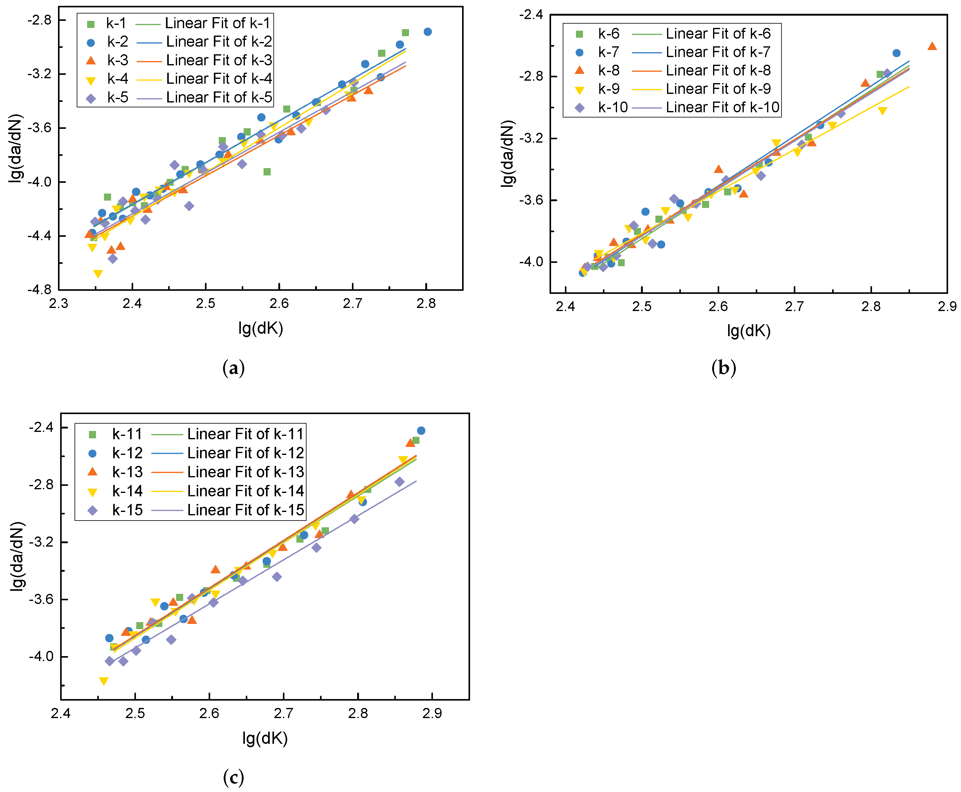
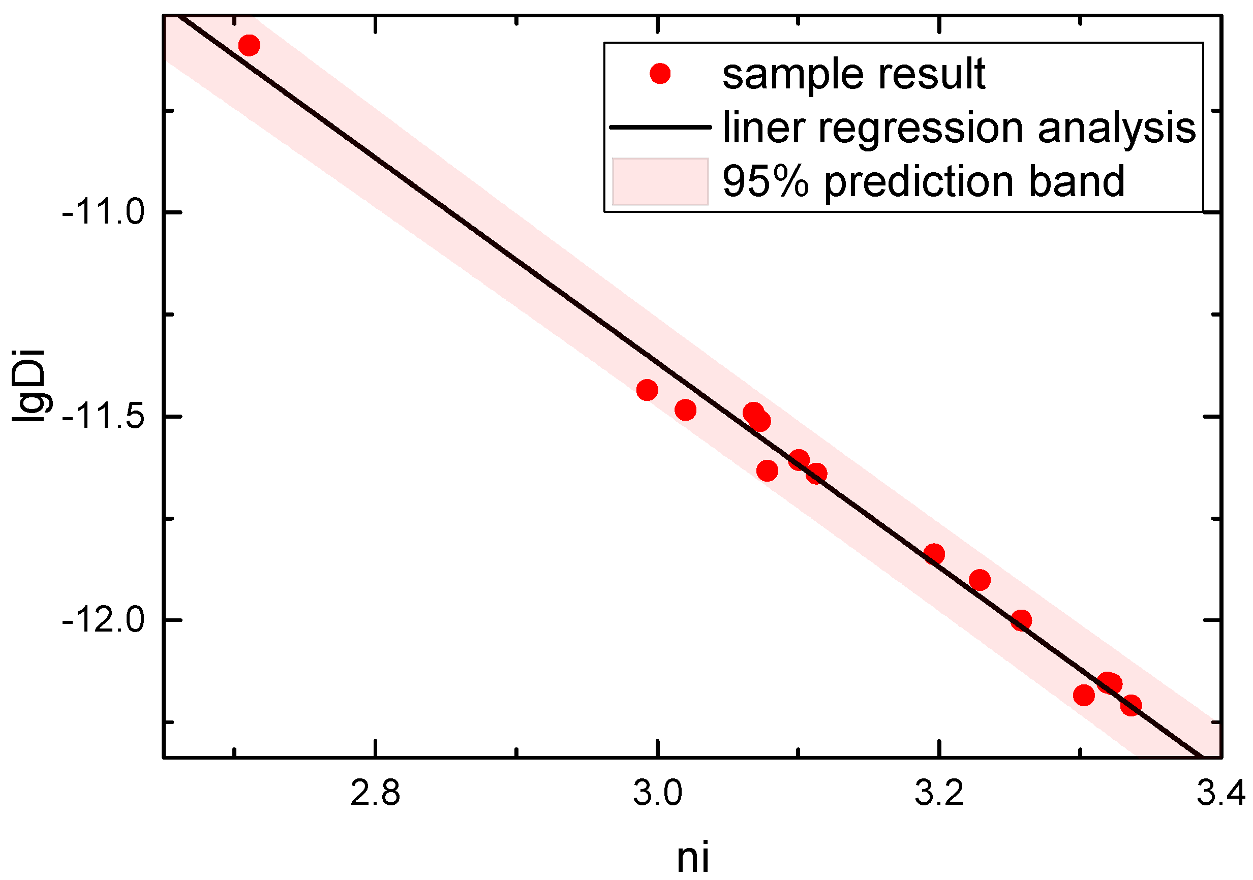
4.3. Processing and Statistics of Crack Propagation Test Results

In the first section, the ( a i , N i ) data of crack growth are shown in Figure 2b–d. In order to establish a random crack growth model, statistical analysis of ( a i , N i ) data is needed to obtain the distribution of random parameters D i and n i .
Firstly, the secant method is used to estimate the crack growth rate d a / d N . In other words, the slope of the connecting line between adjacent data points is taken as the crack growth rate corresponding to the average crack size in the interval.
( d a / d N ) i = ( a i + 1 a i ) / ( N i + 1 N i )
Figure 9a–c show the relationship curve between crack growth rate d a / d N and crack size. It can be seen from these figures that as the crack size increases, the crack growth rate d a / d N is also increasing, and the crack size is positively correlated with the crack growth rate.
Since the pairs formula is a formula to express the relationship between d a / d N and Δ K , it is necessary to obtain the Δ K of the corresponding crack length a after obtaining the relationship between d a / d N and a. Generally, the methods to calculate the stress intensity factor are the handbook method, weight function method [22], finite element method [23], etc. In this paper, the finite element method is used to calculate Δ K .
When the crack size is a, the stress intensity factor ( K m a x ) corresponding to the maximum stress is calculated by FEM (see Section 4.2 for FEM), and then Δ K is calculated by the following formula.
Δ K = K m a x × ( 1 R )
The amplitude of stress intensity factor Δ K corresponding to crack size a of each test piece is calculated by the above method. Then, according to the relationship between the crack size a and the crack growth rate d a / d N shown in Figure 9a–c, the relationship between Δ K and d a / d N is obtained. The log( Δ K ) − log( d a / d N ) curve is shown in Figure 10a–c.
From Equation (8), it can be seen that log( d a / d N ) and log( Δ K ) are linear, so the values of D i and n i of each test piece can be obtained by linear regression analysis.
Linear regression analysis was carried out on the all test pieces, and the results are shown in Figure 11. It can be seen from the figures that log( d a / d N ) has a strong linear relationship with log( Δ K ).
Through linear regression analysis, the crack propagation parameters of all test pieces are obtained, as shown in Figure 12.
Figure 11 and Figure 12 show the the correlation of log( d a / d N ) and log( Δ K ) regression analysis and values of D i and n i of all 15 test pieces, respectively. It can be seen from the correlation that the linear correlation between log( d a / d N ) and log( Δ K ) in all test pieces is very strong, which also proves the validity of the fitted values of D i and n i .
D i ¯ = 3.49 · 10 12 can be obtained from Figure 12. Place D i ¯ into Equation (9) to obtain the value of u i . Since u i satisfies the three-parameter lognormal distribution, it is necessary to estimate the position parameter τ , dispersion parameter α , and shape parameter β of Equation (10) according to the value of u i . In this paper, the above three parameters are estimated by the method of moment estimation. The specific method is as follows.
First, find the sample mean A 1 , the second-order origin moment A 2 , and the third-order origin moment A 3 of the sample u i , which are equal to the estimated values μ 1 ^ , μ 2 ^ , μ 3 ^ of the mean of u i , u i 2 , u i 3 , respectively;
μ 1 ^ = A 1 = 1 n i = 1 n u i μ 2 ^ = A 2 = 1 n i = 1 n u i 2 μ 3 ^ = A 3 = 1 n i = 1 n u i 3
Then, find the mean of the population x, x 2 , x 3 :
E ( x ) = τ + x f ( x ) d x = μ 1 E ( x 2 ) = τ + x 2 f ( x ) d x = μ 2 E ( x 3 ) = τ + x 3 f ( x ) d x = μ 3
where, f ( x ) is a three-parameter lognormal distribution density function; see Equation (10).
Finally, let the population mean μ 1 , μ 2 , μ 3 be equal to the sample mean estimated value μ 1 ^ , μ 2 ^ , μ 3 ^ .
μ 1 = μ 1 ^ μ 2 = μ 2 ^ μ 3 = μ 3 ^
Finally, the parameters are estimated as τ = 2.558 , α = 0.697 , β = 0.134 .
From Figure 12, the relationship curve between log D i and n i can be obtained, as shown in Figure 13. Figure 13 shows that log D i and n i satisfy a linear relationship. The values of l 0 and l 1 in Equation (13) can be obtained by linear regression analysis of the two parameters, l 0 = −2.51, l 1 = −3.84.
After obtaining the above parameters, the values of D i and n i can be randomly obtained by Equations (13) and (14), and the crack growth rate d a / d N can be obtained by substituting D i and n i into Equation (8), and finally random crack growth analysis can be performed.

5. Residual Strength Analysis of MSD Structure

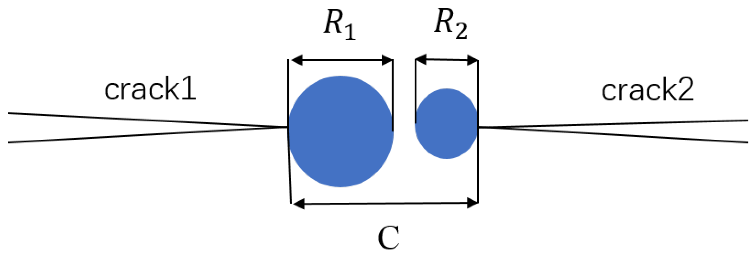
5.1. Plastic Zone Connectivity Criterion

Crack connectivity is the most common failure form of MSD. When plastic zones at the tip of two adjacent cracks come into contact, it is considered that the two cracks are connected. Usually, the structure will be damaged soon after the crack is connected.
As shown in Figure 14, there are two plastic zones at the crack tips. When the two plastic zones are in contact, i.e., when Equation (20) is satisfied, crack 1 and crack 2 are connected.
R 1 + R 2 = C
where R 1 and R 2 are the plastic zone dimensions of crack 1 and crack 2, respectively. C is the crack tip distance of crack 1 and crack 2.
There are two methods to calculate the plastic zone size R: (1) Irwin formula [24]; (2) Dugdale formula [25].
The size of the plastic zone at the crack tip under the plane stress state calculated by the Irwin formula is:
R 1 = 1 π ( K 1 / σ b ) 2 R 2 = 1 π ( K 2 / σ b ) 2
The size of the plastic zone at the crack tip under the plane stress state calculated by the Dugdale formula is:
R 1 = π 8 ( K 1 / σ b ) 2 R 2 = π 8 ( K 2 / σ b ) 2
where K 1 represents the stress intensity factor at the tip of crack 1 and K 2 represents the stress intensity factor at the tip of crack 2. σ b is the yield stress of the material.
K 1 and K 2 in Equation (22) can be obtained by Equation (23):
K 1 = β 1 σ π a 1 K 2 = β 2 σ π a 2
where β 1 and β 2 are the stress intensity factor correction factors at the tips of crack 1 and crack 2, respectively. a 1 and a 2 are the size of crack 1 and crack 2, respectively. σ is the stress on the structure.
The residual strength of the structure is obtained by the Irwin formula:
σ = σ b b a 1 β 1 2 + a 2 β 2 2 β h 2
The residual strength of the structure obtained by the Dugdale formula is:
σ = σ b π 8 b a 1 β 1 2 + a 2 β 2 2 β h 2
In the equation, β h is the stress intensity factor or the Bowie factor of the MSD crack [26].

5.2. Structural Failure Criterion

In engineering practice, crack connection does not mean structural failure and destruction, so other criteria are needed to consider structural failure. In this paper, the fracture mechanics ( K C ) method is used to consider the local unstable fracture of a crack, and the net section criterion is used to consider the failure of a structure.
(1) Fracture mechanics ( K C ) method.
This method is based on linear elastic fracture mechanics. The basic assumption of the guidelines is as follows: when the structure undergoes instability fracture under the applied load, the main crack has a critical stress intensity value. K C is the fracture toughness of the material. When K I > K C , the structure is considered to undergo failure fracture. The formula of stress intensity factor K I is as follows:
K I = σ π a β w β α
where β w is the finite width correction factor; β α is the correction factor of crack interaction.
(2) Net section criterion.
The failure predicted by the net section criterion is based on the amount of material loaded on the structural section. Therefore, the failure load is a function of the yield strength of the material and the number of defects. When the net section stress σ n e t > σ y s , it is considered that the structure fails to break.
σ n e t = P / [ ( W 2 a 2 n × d 2 n × L ) × t ] = σ × ( W n × d ) / ( W 2 a 2 n × d 2 n × L ) .
where σ is the stress; σ n e t is the net section stress; σ y s is the yield strength of the material; W is the width of the metering section; a 2 is the half length of the central main crack (when there is a main crack); n is the number of holes; d is the average diameter of the hole; L is the average half crack length of the MSD crack (the crack length is measured from the hole edge); t is the thickness of the orifice plate.

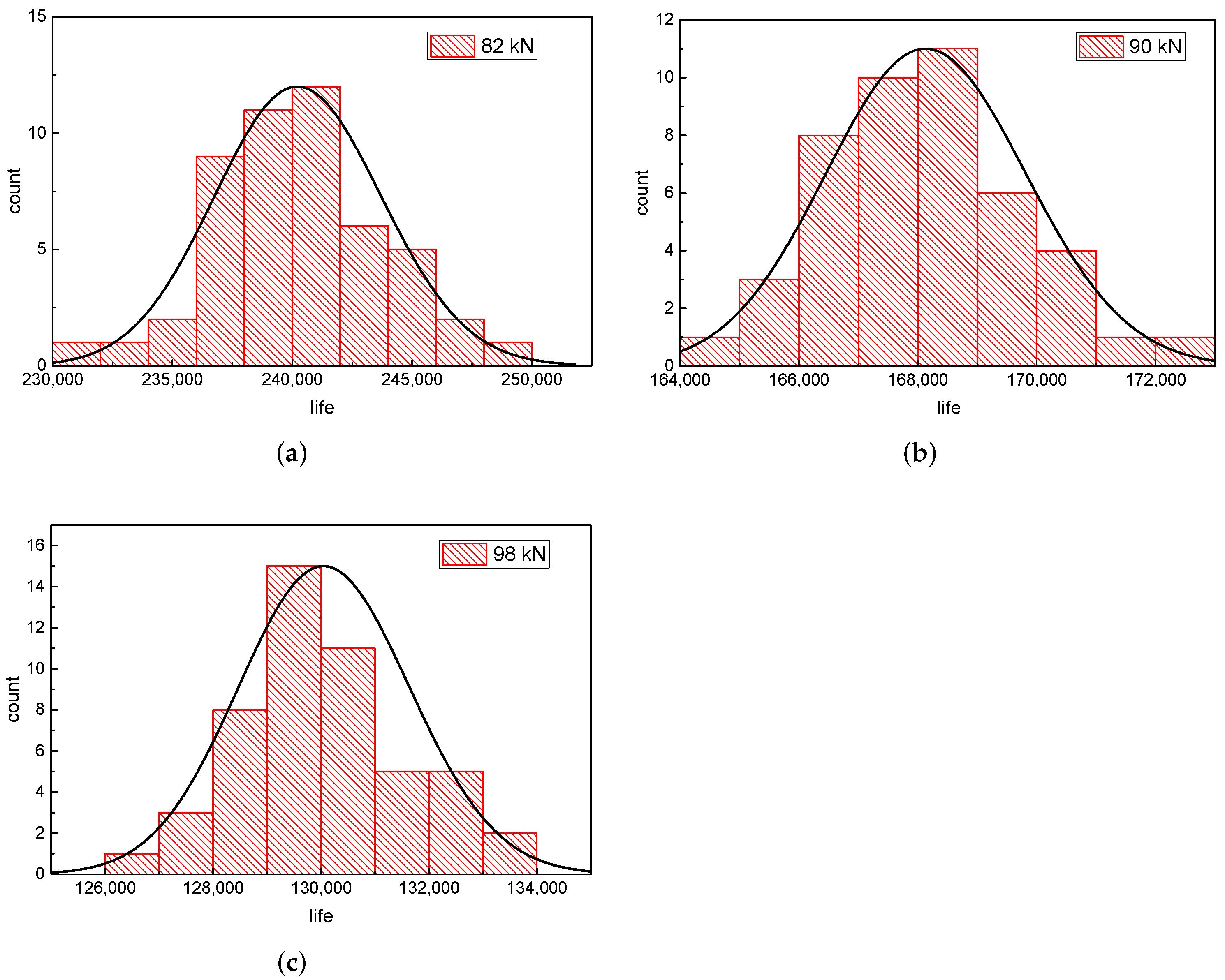
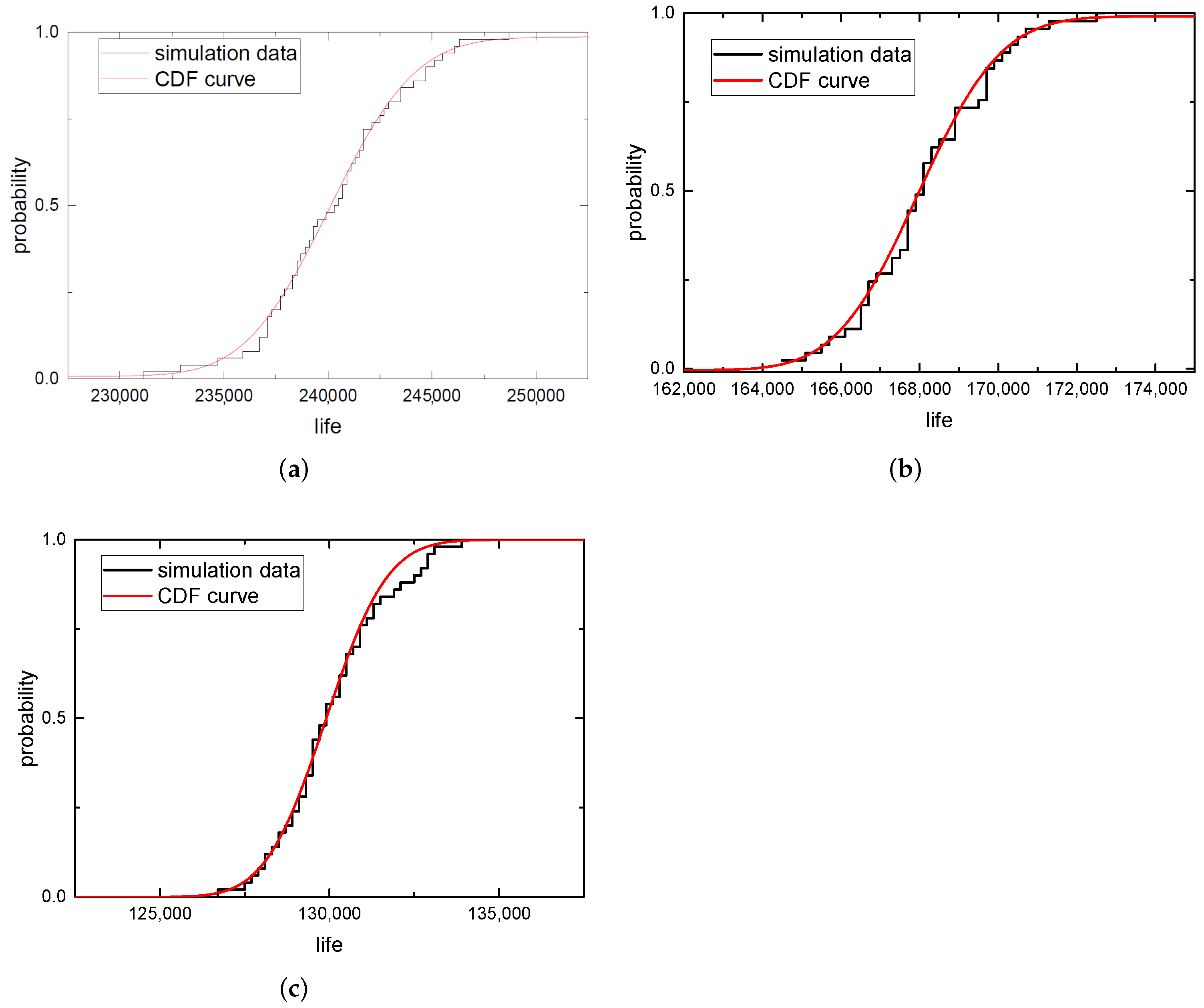
6. Prediction of Structural Life by Monte Carlo Method

The Monte Carlo method, also known as the random sampling technique or statistical test method, is a numerical method based on probability and statistics theory, using random simulation and statistical test methods to find approximate solutions to certain mathematical, physical, and engineering problems [27].
In this paper, the MSD structure random crack initiation model, random variable-based crack growth model, residual strength analysis of MSD structure and other methods, combined with Monte Carlo method, are used to carry out probabilistic analysis of the MSD structure life. The steps are as follows:
  • Determine basic properties such as geometric configuration, material properties, initial crack size, and load spectrum size.
  • According to the test data, obtain the distribution of the parameters describing the dispersion in the random crack initiation and random crack growth models, and estimate the parameters that satisfy the distribution.
  • Use a random number generator to generate a set of random numbers C 0 i j that obey the standard normal distribution. The random number C i j simulating the dispersion of crack initiation is obtained by Equation (3). The initiation life N i j and initiation sequence of cracks at each position are obtained by Equations (3) and (6).
  • For the non-initiation position, fatigue damage will continue to accumulate until the cumulative damage value is 1. For the location of the initiated crack, the random crack propagation analysis is carried out.
  • The random number generator is used to generate a group of random numbers D 0 i j that obey the standard normal distribution. The random parameters D i j and n i j describing the crack growth rate are obtained by Equations (12) and (13), respectively. Then, the Δ K value of each crack tip is obtained by the finite element solution, and the crack growth increment Δ a for a given cycle life Δ N is obtained by substituting into Equation (8).
  • Add Δ a to the original crack length a, update the crack size a, and then give Δ N and find Δ a , and keep cycling. In the process of this cycle, it is continuously determined whether the connectivity criterion and failure criterion are met. If the connectivity criterion is met, the two adjacent cracks are connected. If the failure criterion is met, the structure breaks and fails, and the calculation stops. The simulated structural life is obtained N W F D j .
  • Calculate L times of the above process, i.e., complete L times of Monte Carlo sampling to obtain the results of L structural lives N W F D j ( j = 1 , 2 , , L ) . Through statistical analysis of the calculation results, the logarithmic life mean log N ¯ and logarithmic life standard deviation S log N of the structure can be obtained.

7. Analysis Examples

7.1. Seven-Hole Collinear Plate Test

The typical riveted panel MSD structure of aircraft—a single-row seven-hole collinear panel—was selected for the test, and the calculation method introduced in this paper was analyzed in order to verify the effectiveness of this method. The geometric dimensions of the test piece are shown in Figure 15.
The seven-hole collinear plate test was carried out on a 1000 kN Instron8801 hydraulic fatigue testing machine. There were 9 test pieces in total, and there were 3 test pieces under three stress levels ( P m a x = 82 kN, P m a x = 90 kN, P m a x = 98 kN), respectively. The load spectrum was a constant-amplitude spectrum, the stress ratio was 0.1, and the test loading frequency was 5 Hz. See Figure 16 for test photos of the 7-hole collinear plate.

7.2. Simulation Calculation

A series of calculation methods introduced in this paper, such as the random crack initiation model, random crack propagation model, residual strength analysis, and Monte Carlo method, were compiled into a set of calculation programs, which was used to predict the life of the 7-hole plate shown in Figure 15. Fifty simulated samples were taken at three force levels, P m a x = 82 kN, P m a x = 90 kN, P m a x = 98 kN. The simulation results are shown in Figure 17a–c.
It can be seen from Figure 17a–c that the life of the 7-hole collinear plate basically follows lognormal distribution, and the lognormal distribution curve becomes narrower with the increase in stress level, indicating that the life dispersion becomes smaller with the increase in stress level.
Table 5 shows the comparison between the calculation results and the test results. It can be seen from the table that the structural life obtained by simulation calculation is very close to the test results, indicating that the method described in this paper can accurately predict the life of MSD structures.
Figure 18a–c show the cumulative distribution curve of structural life under three stress levels. The black solid line is the cumulative distribution curve of structural life obtained by 50 groups of simulation sampling, and the red curve is the lognormal cumulative distribution function (CDF) curve based on 50 simulation data. The failure probability and reliability corresponding to a certain life can be obtained through the CDF curve. In particular, the fatigue life when the failure probability is 50%, i.e., WFD average behavior, can be obtained. The average behavior of WFD under three stress levels, P m a x = 82 kN, P m a x = 90 kN, P m a x = 98 kN, is 240,300, 167,900, 129,750, respectively.
The crack growth data obtained from 50 simulations under three stress levels were processed to obtain 50 crack growth curves corresponding to each crack, and the crack growth curves corresponding to the maximum life and minimum life under the same stress level were compared with the test data. Because the cracks in the seven-hole plate were symmetrical from left to right, half of the cracks were taken for analysis. We selected a test piece under each stress level for comparison, and the comparison results are shown in Figure 19.
In Figure 19, “L” stands for left, “R” stands for right, and “crack 1-L” stands for the crack on the left side of hole 1. “Max life” and “min life”, respectively, represent the crack propagation data corresponding to the maximum crack propagation life and the minimum crack propagation life obtained by simulation calculation. It can be seen from the figure that the test data are basically located between the two lines of “max life” and “min life”, which shows that the crack growth model based on random variables established in this paper can successfully predict the actual crack growth.

8. Conclusions

1. In ABAQUS, by defining the crack and the crack tip integral region, setting the singularity of the crack tip, and meshing, the calculation of the stress intensity factor at the crack tip is realized. Through the statistical analysis of the crack propagation data of LY12-CZ aluminum alloy single-hole test pieces, it is found that the variables log D i and n i in the Paris formula log ( d a / d N ) = log D i + n i log ( Δ K ) have a strong linear relationship, which can be expressed as log D i = l 0 · n i + l 1 , where l 0 = −2.51, l 1 = −3.84.
2. The fatigue test data of a single-detail perforated plate are used to estimate the random parameters C i , D i , and n i in the random crack initiation model and crack propagation model. In order to judge structural failure and crack connectivity, the K C criterion, net section criterion, and Swift criterion are adopted. Finally, the randomness of crack initiation and propagation is simulated by Monte Carlo sampling. For the MSD structure, the calculation results show that the structure life obeys a lognormal distribution.
3. Based on the knowledge of fracture mechanics and fatigue statistics, this paper analyzes the whole process of crack initiation, fracture, and structural failure of an MSD structure by using the probability method, and establishes a random crack initiation model and random crack propagation model. The comparison with the test results of a seven-hole collinear plate shows that the calculation results of the method described in this paper are accurate and can accurately predict the life distribution of MSD structures.

Author Contributions

Conceptualization, F.W. and M.T.; methodology, K.L. and S.B.; software, K.L.; validation, K.L., L.Y., and Q.Z.; formal analysis, L.Y.; investigation, W.P.; resources, M.T.; data curation, F.W.; writing—original draft preparation, K.L.; writing—review and editing, K.L.; visualization, W.P.; supervision, F.W.; project administration, M.T.; funding acquisition, M.T. All authors have read and agreed to the published version of the manuscript.

Funding

This research was funded by the National Natural Science Foundation of China (No. 52075232), Aeronautical Science Foundation of China (No. 20182352015 and 201928052009), and Nanjing University of Aeronautics and Astronantics (No. 180603DF01). This research was supported by research on xxx-110 hydraulic pressure energy storage technology of a basic research project.

Institutional Review Board Statement

Not applicable.

Informed Consent Statement

Not applicable.

Data Availability Statement

The data presented in this study are available on request from the corresponding author.

Acknowledgments

The authors gratefully acknowledge the reviewers for their careful work and thoughtful suggestions, which helped to improve this paper substantially. Special thanks to Mingbo Tong for the guidance and Fangli Wang for the revision.

Conflicts of Interest

The authors declare no conflict of interest.

References

  1. Horst, P. Widespread fatigue damage—An issue for aging and new aircraft. In Key Engineering Materials; Trans Tech Publications Ltd.: Schwyz, Switzerland, 2006; Volume 324, pp. 1–8. [Google Scholar]
  2. Federal Aviation Administration. Aging aircraft program: Widespread fatigue damage, proposed rule. Fed. Regist. 2006, 74, 19927–19951. [Google Scholar]
  3. Xi, W.; Zhao, J.J.; Yao, W.X. Probability distribution analysis model of crack initiation life for widespread fatigue damage. China Sci. 2016, 11, 576–580. [Google Scholar]
  4. Yan, X.Z.; Wang, S.N.; Huang, H.C. Probability analysis method for aircraft structures containing multiple site damage. J. Mech. Strength 2012, 34, 881–885. [Google Scholar]
  5. Ai, Y.; Zhu, S.P.; Liao, D.; Correia, J.A.F.O.; Souto, C.; De Jesus, A.M.P.; Keshtegar, B. Probabilistic modeling of fatigue life distribution and size effect of components with random defects. Int. J. Fatigue 2019, 126, 165–173. [Google Scholar] [CrossRef]
  6. Jung-Hoon, K.; Thanh, C.D.; Goangseup, Z. Probabilistic fatigue integrity assessment in multiple crack growth analysis associated with equivalent initial flaw and material variability. Eng. Fract. Mech. 2016, 156, 182–196. [Google Scholar]
  7. Wang, S.; Liu, M.B.; Wang, G.l. Experimental study and finite element analysis of widespread damage. Acta Aeronaut. Astronaut. Sin. 2010, 31, 1578–1583. [Google Scholar]
  8. Ray, A.; Patankar, R. A stochastic model of fatigue crack propagation under variable amplitude loading. Eng. Fract. Mech. 1999, 62, 477–493. [Google Scholar] [CrossRef]
  9. Riahi, H.; Bressolette, P.; Chateauneuf, A. Random fatigue crack growth in mixed mode by stochastic collocation method. Eng. Fract. Mech. 2010, 77, 3292–3309. [Google Scholar] [CrossRef]
  10. Edson, D.L.; André, T.B.; Wilson, S.V. On the performance of response surface and direct coupling approaches in solution of random crack propagation problems. Struct. Saf. 2011, 33, 261–274. [Google Scholar]
  11. Salimi, H.; Kiad, S.; Pourgol-Mohammad, M. Stochastic Fatigue Crack Growth Analysis for Space System Reliability. ASCE-ASME J. Risk Uncertain. Eng. Syst. Part B Mech. Eng. 2017, 4, 1–31. [Google Scholar] [CrossRef]
  12. Pyo, C.R.; Okada, H.; Atluri, S.N. An elastic-plastic finite element alternating method for analyzing wide-spread fatigue damage in aircraft structures. Comput. Mech. 1995, 16, 62–68. [Google Scholar] [CrossRef]
  13. Wu, L.; Sun, Q. Study on semi analytical numerical algorithm of stress intensity factor of structure with MSD. J. Northwestern Polytech. Univ. 2003, 21, 214–217. [Google Scholar]
  14. Swift, T. Damage tolerance capability. Int. J. Fatigue 1994, 16, 75–94. [Google Scholar] [CrossRef]
  15. Ge, S.; Li, Z.; Zhang, J.G. Residual strength of unreinforced aluminum alloy panel with multiple damages. Acta Aeronaut. Astronaut. Sin. 2008, 29, 411–415. [Google Scholar]
  16. Bert, L.S.; Perry, A. Strength of 2024-T3 Aluminum Panels with Multiple Site Damage. J. Aircr. 2000, 37, 325–331. [Google Scholar]
  17. Wang, C.S.; Zhang, J.Y.; Bao, R. Test study on residual strength of aluminum alloy plate containing MSD. J. Aeronaut. Mater. 2007, 27, 346–350. [Google Scholar]
  18. Sergey, S.; Roman, K. Probabilistic mothod for the analysis of widespread fatigue damage in structures. Int. J. Fatigue 2005, 27, 223–234. [Google Scholar]
  19. Gao, Z. Fatigue Applied Statistics, 3rd ed.; National Defense Industry Press: Beijing, China, 1986. [Google Scholar]
  20. Paris, P.; Erdogan, F. A critical analysis of crack propagation laws. ASM Trans. J. Basic Eng. 1963, 85, 528–534. [Google Scholar] [CrossRef]
  21. Sun, H.; Dong, D.; Chen, L. Prediction of Random Crack Propagation Life of Multi-damaged Pore Structures. Sci. Technol. Eng. 2019, 19, 278–283. [Google Scholar]
  22. Kou, K.P.; Cao, J.L.; Yang, Y. Weight Function Method for Stress Intensity Factors of Semi-Elliptical Surface Cracks on Functionally Graded Plates Subjected to Non-Uniform Stresses. Materials 2020, 13, 3155. [Google Scholar] [CrossRef]
  23. Hsin, J.H.; John, H.L.P.; Kin, S.T. Stress intensity factors for fatigue analysis of weld toe cracks in a girth-welded pipe. Int. J. Fatigue 2016, 87, 279–287. [Google Scholar]
  24. Irwin, G.R. Analysis of stresses and strains near the end of a crack traversing a plate. ASME J. Appl. Mech. 1957, 24, 361–364. [Google Scholar] [CrossRef]
  25. Dugdale, D.S. Yielding of steel sheets containing slits. J. Mech. Phys. Solids 1960, 8, 279–287. [Google Scholar] [CrossRef]
  26. Grandt, A.F. Stress intensity factors for some through-cracked fastener holes. Int. J. Fract. 1975, 11, 283–294. [Google Scholar] [CrossRef]
  27. Kebir, H.; Roelandt, J.M.; Gaudin, J. Monte Carlo simulations of life expectancy using the dual boundary element method. Eng. Fract. Mech. 2001, 68, 1371–1375. [Google Scholar] [CrossRef]
Figure 1. Geometric dimensions of single-hole test piece.
Aerospace 09 00215 g001
Figure 2. (a) Crack initiation life and S N i n i t curve. (b) Crack growth curve of 15.20 kN. (c) Crack growth curve of 18.24 kN. (d) Crack growth curve of 19.76 kN.
Aerospace 09 00215 g002
Figure 3. MSD structure chart.
Aerospace 09 00215 g003
Figure 4. Hole crack definition model diagram.
Aerospace 09 00215 g004
Figure 5. (a) Node offset of 8-node element. (b) ABAQUS crack singularity setting.
Aerospace 09 00215 g005
Figure 6. Meshing of crack tip.
Aerospace 09 00215 g006
Figure 7. Single-hole plate geometry model.
Aerospace 09 00215 g007
Figure 8. (a) Stress nephogram of a = 2 mm. (b) Stress nephogram of a = 5 mm. (c) Stress nephogram of a = 10 mm.
Aerospace 09 00215 g008
Figure 9. (a) a d a / d N curve of 15.20 kN. (b) a d a / d N curve of 18.24 kN. (c) a d a / d N curve of 19.76 kN.
Aerospace 09 00215 g009
Figure 10. (a) log( Δ K ) − log( d a / d N ) curve of 15.20 kN. (b) log( Δ K ) − log( d a / d N ) curve of 18.24 kN. (c) log( Δ K ) − log( d a / d N ) curve of 19.76 kN.
Aerospace 09 00215 g010aAerospace 09 00215 g010b
Figure 11. (a) log( d a / d N ) and log( Δ K ) linear regression analysis of 15.20 kN. (b) log( d a / d N ) and log( Δ K ) linear regression analysis of 18.24 kN. (c) log( d a / d N ) and log( Δ K ) linear regression analysis of 19.76 kN.
Aerospace 09 00215 g011
Figure 12. Values of D i and n i of test pieces.
Aerospace 09 00215 g012
Figure 13. log D i and n i linear regression analysis.
Aerospace 09 00215 g013
Figure 14. Diagram of plastic zone at crack tip.
Aerospace 09 00215 g014
Figure 15. (a) Geometric dimensions of 7-hole plate. (b) Physical drawing of 7-hole plate.
Aerospace 09 00215 g015
Figure 16. Site drawing of seven-hole collinear plate test.
Aerospace 09 00215 g016
Figure 17. (a) Life distribution of P m a x = 82 kN. (b) Life distribution of P m a x = 90 kN. (c) Life distribution of P m a x = 98 kN.
Aerospace 09 00215 g017
Figure 18. (a) Cumulative life span distribution curve of P m a x = 82 kN. (b) Cumulative life span distribution curve of P m a x = 90 kN. (c) Cumulative life span distribution curve of P m a x = 98 kN.
Aerospace 09 00215 g018
Figure 19. (a) Comparison between predicted and experimental values of crack propagation data of P m a x = 82 kN. (b) Comparison between predicted and experimental values of crack propagation data of P m a x = 90 kN. (c) Comparison between predicted and experimental values of crack propagation data of P m a x = 98 kN.
Aerospace 09 00215 g019
Table 1. Material parameters of LY12-CZ.
E/MPaμ K C σ s /MPa
6.8 × 10 3 0.33100339
Table 2. Fatigue test plan for single-detail perforated plates.
P max / kN RfNumberNumber of Test Pieces
15.200.15 Hzk1–k55
18.240.15 Hzk6–k105
19.760.15 Hzk11–k155
Table 3. Random crack initiation parameters of LY12-CZ.
m log C i ¯ S log C i
4.9313.120.05
Table 4. Comparison of stress intensity factors calculated by ABAQUS and handbook.
a (mm)ABAQUSHandbookError (%)
2554.4548.71.04
5721.7717.40.60
101179.01173.90.43
Table 5. Comparison between the calculation results and the test results of the seven-hole plate.
F/kN log N ¯ S log N log N ¯ S log N
825.3810.0065.3900.014
905.2250.0045.2080.027
985.1140.0055.1010.030
Publisher’s Note: MDPI stays neutral with regard to jurisdictional claims in published maps and institutional affiliations.

