Preliminary Analysis of Compression System Integrated Heat Management Concepts Using LH₂-Based Parametric Gas Turbine Model

Abstract

The investigation of the various heat management concepts using LH₂ requires the development of a modeling environment coupling the cryogenic hydrogen fuel system with turbofan performance. This paper presents a numerical framework to model hydrogen-fueled gas turbine engines with a dedicated heat-management system, complemented by an introductory analysis of the impact of using LH₂ to precool and intercool in the compression system. The propulsion installations comprise Brayton cycle-based turbofans and first assessments are made on how to use the hydrogen as a heat sink integrated into the compression system. Conceptual tubular compact heat exchanger designs are explored to either precool or intercool the compression system and preheat the fuel to improve the installed performance of the propulsion cycles. The precooler and the intercooler show up to 0.3% improved specific fuel consumption for heat exchanger effectiveness in the range 0.5–0.6, but higher effectiveness designs incur disproportionately higher pressure losses that cancel-out the benefits.

1. Introduction

The development of commercial air transportation over the coming decades requires greater consideration of its environmental impact concerning the emanations of CO₂ and non-CO₂ emissions [1,2,3,4]. As part of the effort to reduce aviation’s climate impact, new sustainable and eco-friendly fuels emitting less CO₂, such as Liquefied Bio Gas (LBG), or even a carbon-free fuel such as Liquid Hydrogen (LH₂) [5,6,7] are being considered. Liquid hydrogen has been the prime fuel for space rocket engines and it has been field-tested in some experimental aircraft. Recent conceptual studies on the usage of hydrogen in commercial aircraft have confirmed its potential to reduce the climate impact of aviation [8,9,10]. A comparison of exhaust emissions of kerosene and liquid hydrogen provided by [11,12] encourages the utilization of LH₂ as a sustainable alternative fuel for aviation. It eliminates carbon dioxide, carbon monoxide, sulfur oxides, unburned hydrocarbons, and soot emissions (other than those generated through oil consumption). It also provides an improved combustion stability range for lean mixtures, hence contributing to a reduction in NO_x emissions; however, the hydrogen-fueled subsonic aero-engine will emit about three-times more water vapor than the Jet A counterpart [13] and the direct and indirect impact of water vapor on the climate must also be taken into account [13,14]. Still, even while accounting for all the above mentioned merits, until recently hydrogen has not been considered economically viable for civil aviation. The main reasons being, the technological challenges required to develop an operable hydrogen powered aircraft, and the lack of a green LH₂ infrastructure [15].

Although replacing fossil-based fuel by liquid hydrogen might seem promising from an environmental perspective, it will challenge many established practices related to fuel systems, materials, airframe design, and propulsion technologies. For instance, the relatively lower volumetric energy density of hydrogen (about 24% that of Jet A) will result in larger volume requirements for the airframe and consequent penalties in aerodynamic performance. In addition, the complexity of hydrogen storage in terms of insulation and supporting structures will result in additional weight penalties. The lower performance will penalize the aircraft energy efficiency, which tends to increase operating costs. On the other hand, at the engine level, the combination of liquid hydrogen’s cryogenic storage temperature and relatively high specific heat capacity enables the hydrogen cooling capacity to be exploited to improve the propulsion system thermal efficiency. In the following section, the potential and synergies of using hydrogen in the engine heat-management system are discussed in more detail.

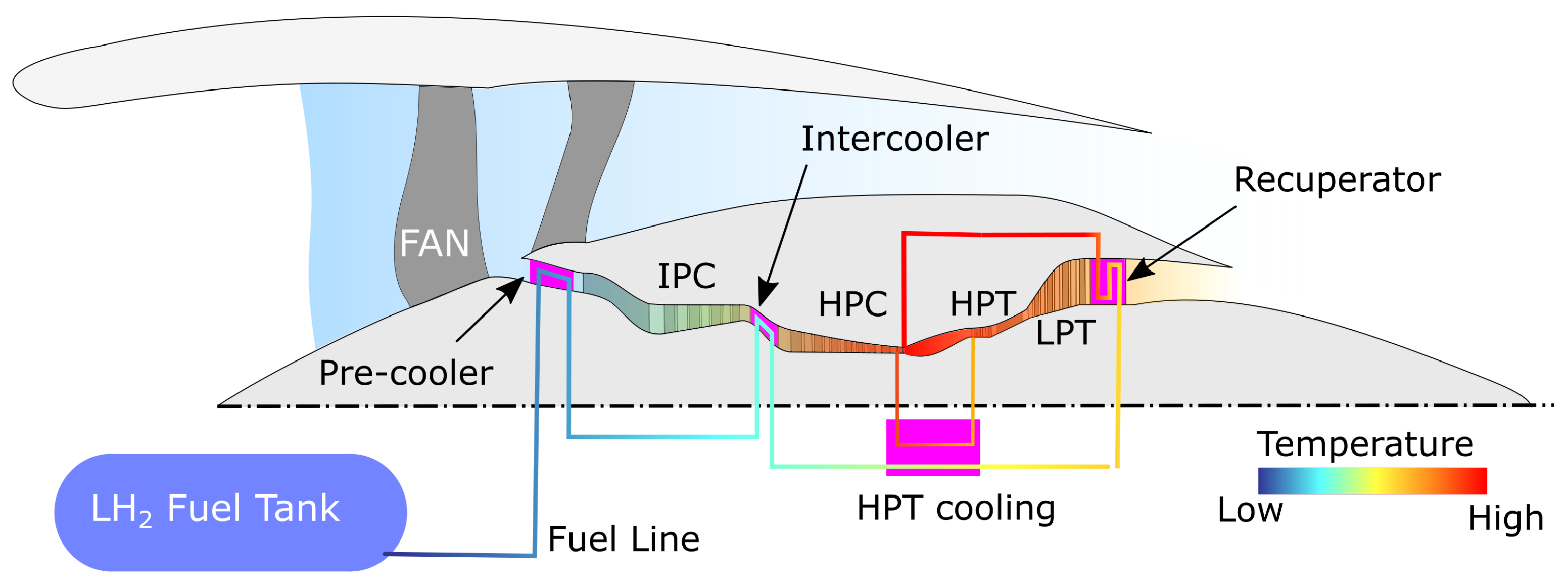
Heat Management Potential

Since liquid hydrogen is stored at cryogenic temperatures, it can undergo a large temperature variation on its way to the combustion chamber. This, associated with the fact that hydrogen has an exceptionally high heat capacity, means that the amount of heat that can be taken up is substantial. As an example, assume that the tank is filled with hydrogen at 25 K and the fuel absorbs heat up to 800 K entering the combustor. The heat added per kilogram of fuel (MJ/kg) corresponds to about 9% of the hydrogen lower fuel heating value (120 MJ/kg). Hence, theoretically, in a loss-free system, the maximum potential is a 9% reduction in specific fuel consumption (SFC). It should be noted that the aforementioned 9% improvement potential is only related to changes in fuel temperature and consequent increase in effective heating value; however, heat exchangers can be strategically located in the engine core to use heat management to maximize engine efficiency, and therefore achieve additional fuel-burn benefits. In the design process of the different heat exchangers, in addition to the impact in performance caused by the location in the gas path, weight and volume are important parameters that must be carefully taken into consideration. A reduction of approximately 6% in fuel consumption while increasing the specific thrust has been reported in previous studies [16]. The resulting heat-management system is therefore integral to the fuel supply and propulsion systems, where it delivers the hydrogen with adequate pressure and temperature to the combustion chamber, while providing cooling in key engine locations (e.g., compression system, turbine cooling air, and engine exhaust). A schematic illustration of a possible fuel heat-management system integrated into the propulsion system is illustrated in Figure 1.

Among various alternatives for the fuel heat management architectures in the LH₂ engine’s cycle [5,12,17], four possibilities arise:

• Pre-cooling: The precooler is located between the fan and intermediate-pressure compressor (IPC). It increases the fuel temperature before entering the combustion chamber and decreases the IPC and HPC work by cooling the core flow before compression.
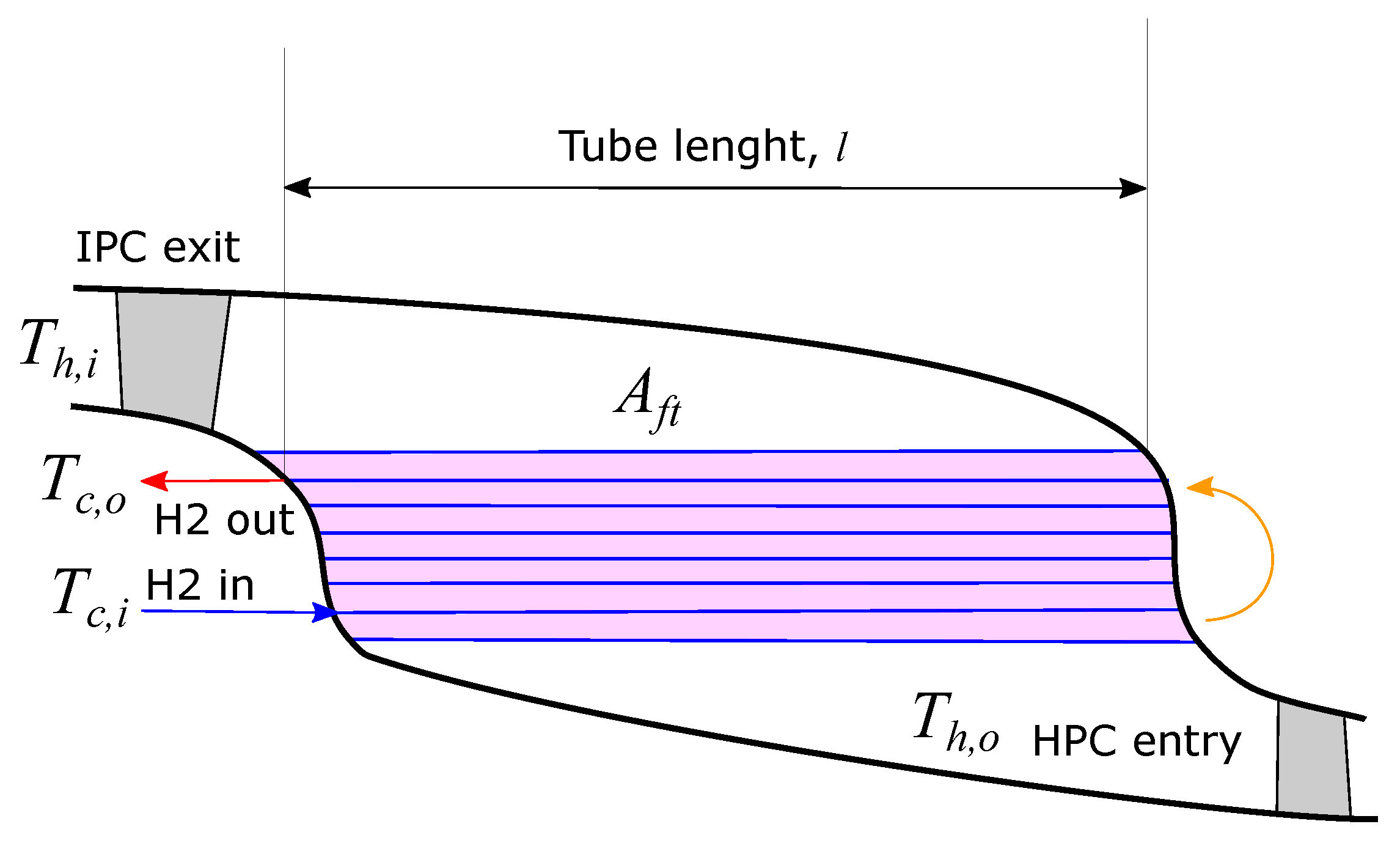
• Intercooling: The intercooler is placed between the IPC and the high-pressure compressor (HPC). Similar to precooling, it raises the fuel temperature before entering the combustion chamber and reduces the HPC work by cooling the compressed airflow. Intercooling and precooling also enable an increase in core-specific work and allow for higher pressure ratios in the compression system before violating HPC discharge temperature limits. Another possible advantage arising for both pre- and intercooling is the possibility of reducing the combustor inlet temperature for a given OPR, which will curb NO_x emissions. A challenge with both concepts is the risk of ice formation in the presence of humid air, which could cause a partial or complete blockage of the engine core flow.
• Cooled-cooling air: The main task of the high-pressure turbine (HPT) cooling is to reduce the temperature of the cooling air extracted from the HPC and used to cool the HPT. The potential is to improve the engine efficiency by reducing the amount of secondary air flows for a given turbine metal temperature limit.
• Recuperation: The recuperator is the main source of LH₂ fuel heating before injection into the combustor. Among the other heat exchangers, it has the greatest potential for increasing the fuel temperature.

The precooler and intercooler also allow increases in the overall pressure ratio (OPR) and core-specific power without exceeding any cycle temperature limit.

In this paper, the required tools and methods implemented to simulate the fuel architecture and heat-management system are presented and discussed. Additionally, the individual impact of the precooler and intercooler concepts on the performance of the hydrogen-fueled engine were investigated in a parametric study.

2. Engine Performance Simulation

The investigation of the various heat management concepts using LH₂ requires the development of a modeling environment coupling the cryogenic hydrogen fuel system and turbofan performance. All propulsion modeling carried out for this work was implemented in Chalmers University’s in-house gas turbine modeling tool GESTPAN [18]. In addition to basic performance modules commonly available in most performance tools, links exist to external codes for conceptual design and weight estimates [19,20]. The GESTPAN code is a FORTRAN 90 implementation supporting both steady state and transient modeling and is general in the sense that new gas turbine models can be wired-up, by freely connecting components, to configure a propulsion system. This allows the tool to refine a certain subsystem, connect it in its normal style, and model a refined zoomed subsystem within a “normal” gas turbine model, for instance for a turbofan engine. This makes the tool ideal for refining existing gas turbine models to include more advanced fuel heat-management systems and couple them to the normal air breathing combustion models.

Three additional steps are needed when extending gas turbine performance modeling tools for simulations with cryogenic fuels:

• New combustion products tables are needed to complement conventional kerosene tables normally stored in performance codes;
• The integration of detailed modeling for the heat-management system as the cryogenic fuel flows from the tank to the combustor chamber;
• Means to model and manage heat between the fuel system and the propulsion system.

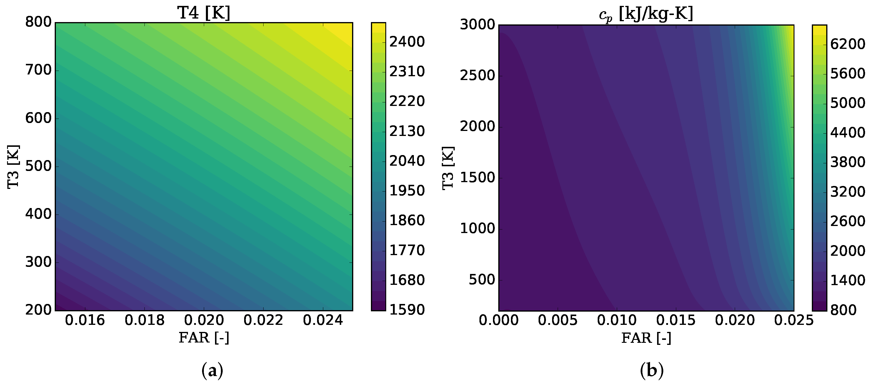
2.1. Combustion Modeling

The first step consists of performing a relatively well-established procedure typically comprising generating new temperature dependent tables for key properties using dedicated combustion software such as the chemical equilibrium software CEA [21]. Thermodynamic tables for the relevant properties, such as enthalpy, entropy, specific heat, and specific heat ratio, are then produced using an interface that automates data generation. Figure 2 shows contour maps illustrating two thermodynamic interpolation tables used in GESTPAN to calculate: (a) temperature rise in the combustor with varying inlet temperature and fuel air ratio (FAR); (b) variation of c_p with fuel air ratio and temperature.

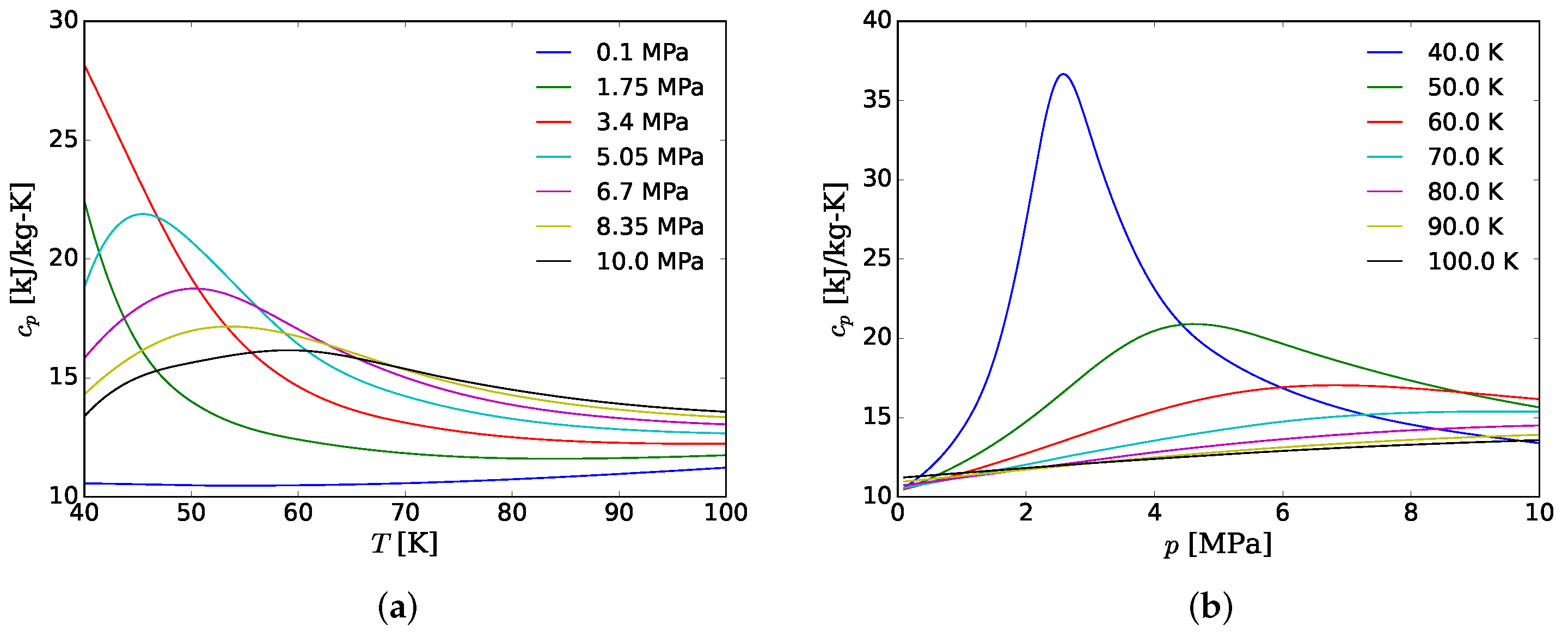
2.2. Detailed Modeling of Real Gases

The second step, pure fuel modeling, requires thermodynamic information about the fuel over a very large range, ranging from cryogenic conditions to temperatures considered the maximum for entering the combustor. Here, the extensively used software REFPROP [22] was applied. Modeling the thermodynamics of gases close to the saturation line poses additional difficulties. Most methods used to represent gas data in performance codes are tailored to physics changing rather slowly in the underlying parameters; however, close to the saturation line and especially close to the critical point, changes are often quite rapid, and accurate representation using standard spline representation may not be satisfactory. REFPROP has, over the years, developed experience in how to best represent fluids accurately around the critical point and it would be reasonable to assume that a direct use of the REFPROP routines linked to the performance code would be the best choice; however, due to speed requirements on REFPROP code, iterative schemes have been included using analytical derivatives of functions. These tend to limit the resolution of the functions, and although the software works perfectly in stand-alone mode, a directly linked version may fail to work with standard iteration numeric. Hence, the internal iteration schemes of REFPROP have been updated to incorporate methods based on bracketing solutions and using only functional evaluations. These methods are slower, resulting in a marginal slow down to the execution, but they are virtually noise-free and make normal gas turbine solutions procedures work well in practice. More specifically, the REFPROP function TPRHO was updated to have a more robust and accurate iteration scheme available if the simulation close to the critical point is being performed. An example of thermodynamic data calculated in GESTPAN for hydrogen is shown in Figure 3. More specifically, a variation of heat capacity with temperature and pressure for pure hydrogen is plotted. A large variation of properties occurs close to the critical temperature of 33 K (not present in the plot).

2.3. Modeling of Coupled Heat Management Systems

The third step, namely heat transfer between the fuel supply and the main engine, poses the greatest modeling challenge. This makes traditional design and off-design simulations of the system substantially more complex to implement. The two flows merging in the main combustor will potentially have exchanged significant amounts of heat prior to fuel injection. Clearly, the heat transferred to the hydrogen will be of a magnitude influencing the thermodynamic state of the combustion products. Preheating the fuel from a cryogenic condition of around 25 K, possibly all the way up to 800–1000 K results in, even if a typical fuel air ratio for hydrogen combustion will not be more than 1%, a 140 K change in temperature of the working gas.

Conventional software for gas turbine modeling manages the fact that a system of non-linear equations needs to be solved by providing very good starting estimates for the solution. Having a thermodynamic design process indirectly solves this numerical problem. In fact, the design point could be a converged off-design point and hence the method has a built-in solution for defining the first converged point. There is no numerical procedure that promises to achieve this for a general problem. With two separate flows, establishing an “on-design” explicit scheme is not possible. It would be possible to iterate a sequence of converged solutions. This would however be numerically challenging and inefficient since the number of nested iterations in a normal gas turbine code is already at least two, but frequently three or even four. Local iterations to establish thermodynamic gas properties, iterative schemes for Reynolds number corrections, etc., are commonplace in gas turbine simulation software. Nested around these functions is normally a Newton solver, usually with a secant method for solution, but brute-force Newton is still in use in some codes. Many optimizers are iterative, and optimization is a common task for gas turbine simulations. When cycles are being optimized another level of iteration is required. In addition, many times the thermodynamic design itself is iterative, matching a thrust or similar. Hence, up to four nested iterations already exist in state-of-the-art gas turbine simulation software. It is not practical to add a fifth level. The already large number of nested iterations poses numerical requirements many times unknown to users and even to developers, rendering many very efficient optimization methods useless or impractical purely for not fulfilling the numerical requirements of the underlying gas turbine model. To summarize: it is not desirable to add further levels of iterations caused by separate fuel flow systems. This problem led to the conclusion that the best way to integrate the fuel heat-management system directly is to add additional equations to the thermodynamic design point iterations. For instance, simultaneously varying gas turbine mass flow to match a thrust requirement and iterating the fuel flow in the heat-management system does not increase the number of iteration levels; it merely adds an extra equation to the design iteration system.

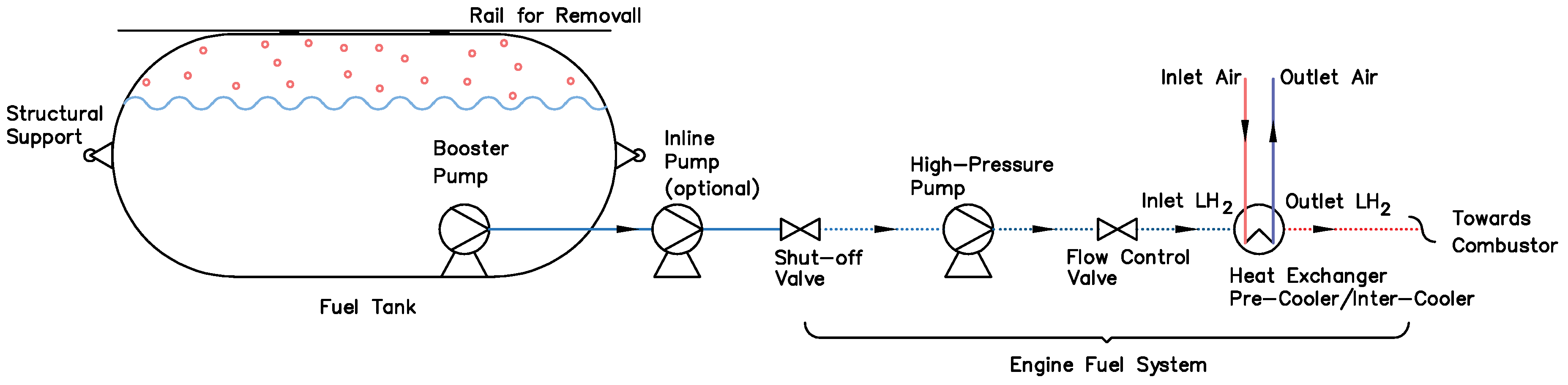
2.4. Fuel Distribution System

Similar to a conventional Jet A fueled aircraft, the main task of the fuel system for the cryogenic fueled aircraft is to deliver the H₂ with appropriate pressure and temperature to the engines for a specified fuel flow. The fuel distribution system, illustrated in Figure 4, comprises different components including a tank-mounted pump system (booster pump), an inline pump, shut-off valves, and the engine-mounted pump. The parameters affecting the fuel distribution line are the pipeline diameter and insulation thickness. Technically, these parameters affect the fuel pressure drop (compensated by the tank-mounted and inline pumps) and heat leakage per unit length as well as pipeline weight. The small pipe size decreases the pipeline weight, but it increases the pressure drop (especially for maximum fuel flow rate) requiring a more powerful pump to overcome. On the other side, apart from minimizing the heat loss, manufacturing/installation cost and maintenance cost, the criterion for the insulation type of the fuel distribution pipeline is not to have ice accumulation outside of the insulation or on components adjacent to the pipes and chilled by them. This may require a ventilation system around the pipes, preferably with a dry inert gas from an onboard inert gas system.

The delivery pressure at the outlet of the fuel distribution system is therefore calculated as:

$$p_{delivery}=p_{tank}{\mathsf{\Pi }}_{bs}{\mathsf{\Pi }}_{inline}{\mathsf{\Pi }}_{engine}-\mathsf{\Delta }{p}_{line},$$

(1)

where $p_{tank}$ is the saturation pressure in the tank and ${\mathsf{\Pi }}_{bs}$, ${\mathsf{\Pi }}_{inline}$, and ${\mathsf{\Pi }}_{hp}$ denote the pressure ratio across the booster pump, inline pump, and engine-mounted pump, respectively. The feed line pressure loss is given by:

$$\mathsf{\Delta }{p}_{line}=f_d\left({\displaystyle \frac{{\rho }_{L{H}_2}}{2}}\right)\left({\displaystyle \frac{v^2}{D_h}}\right)L,$$

(2)

where ${\rho }_{L{H}_2}$, L, v, and $D_h$ are the density of liquid hydrogen, the feed pipeline length, the mean flow velocity in the feed pipeline and the hydraulic diameter of the feed line, respectively. The pressure losses across the different valves in the system are not considered in the present study, although they need to be evaluated when a the full architecture of the fuel distribution system is established. The friction factor $f_d$ is approximated by Haaland’s correlation [23],

$$\frac{1}{f_d^{1/2}}=-1.8log[\frac{6.9}{Re}+{\left(\frac{\zeta /d}{3.7}\right)}^{1.11}],$$

(3)

where d is the fuel line diameter, $Re$ is the tube diameter based Reynolds number and $\zeta$ is the wall roughness height.

In addition to the pressure loss, the enthalpy increase in the fuel system is required,

$$h_{delivery}=\mathsf{\Delta }{h}_{hp}+h_{tank}+\mathsf{\Delta }{h}_{bs}+\mathsf{\Delta }{h}_{inline}+\mathsf{\Delta }{h}_{motor}+\mathsf{\Delta }{h}_{line},$$

(4)

where the enthalpy rise due to heat ingress is,

$$\mathsf{\Delta }{h}_{line}={\displaystyle \frac{q_{L}L}{\dot{m}}},$$

(5)

The variables $q_L$, L, and $\dot{m}$ represent the feed line heat flux per unit length, the feed pipeline length, and the fuel flow rate, respectively. In this study, it is assumed that $q_L=20$ [W/m]. The enthalpy variation across the different pumps is estimated assuming the respective pump efficiency and using REFPROP to calculate the reversible process enthalpy states for the prescribed inlet pressure, pressure ratio, and inlet entropy,

$$\mathsf{\Delta }h=\frac{\mathsf{\Delta }{h}_{ideal}}{\eta },$$

(6)

In the present study, it is assumed that ${\eta }_{bs}=0.70$, ${\eta }_{inline}=0.85$, ${\eta }_{hp}=0.85$, and ${\eta }_{motor}=0.90$.

2.5. Quantifying Installation Effects

In order to quantify the engine performance together with the installation effects, a modified Thrust Specific Fuel Consumption (hereafter called installed TSFC, $\overline{\mathrm{TSFC}}$) is introduced. The new parameter accounts for variations in engine performance, weight, and nacelle size.

$$\overline{\mathrm{TSFC}}={\displaystyle \frac{\mathrm{TSFC}·F_n}{F_n-\left(D_{Nacelle}+D_{Engine}\right)}},$$

(7)

where $F_n$, $D_{Nacelle}$, and $D_{Engine}$ denote net thrust, nacelle drag, and the drag attributable to the engine’s weight, respectively,

$$D_{Engine}={\displaystyle \frac{m_{Engine}·g}{{\left(L/D\right)}_{\mathrm{Nom}.}}},$$

(8)

where $m_{Engine}$, g, and ${\left(L/D\right)}_{\mathrm{Nom}.}$ are the engine’s mass, gravity constant, and nominal aircraft lift to drag ratio at cruise, respectively.

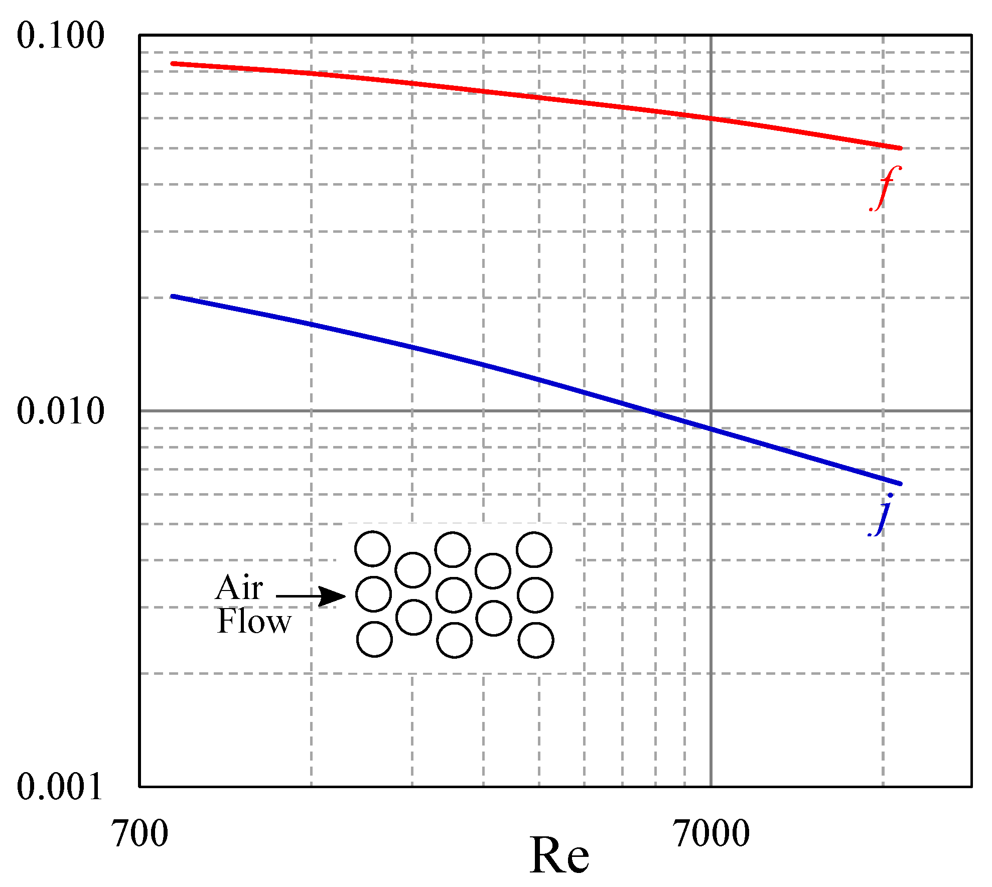
2.6. Heat Exchanger Performance and Conceptual Design

The advantage of LH₂ in terms of cryogenic storage temperature and high specific heat capacity results in an improved cooling capacity relative to conventional fuels. Adequate heat exchanger technology is therefore required to make use of such benefits. One example of an heat exchanger integral to the compressor interconnecting duct is illustrated in Figure 5. In a multi-spool gas turbine, the annular interconnecting ducts (ICD) are used to connect the low/intermediate-pressure compressor to the high-pressure compressor. From an aero-perspective, the ICD should be designed to transfer the flow radially with minimal losses and to provide a uniform temperature and pressure distribution at the HPC inlet. The designer will also aim for a shorter duct in axial length to reduce the engine length, hence reducing weight and drag. The concept shown in Figure 5 allows for a very aggressive area variation between the IPC exit and heat exchanger inlet, allowing for a significant reduction in gas velocity to minimize the external pressure loss. The integration of the heat exchanger in the duct also allows for a more aggressive duct design in terms of radial offset while avoiding possible flow separation. The design of such a heat exchanger is a complex task requiring aerodynamic optimized designs of the diffuser duct (i.e., between the IPC exit and heat exchanger inlet), heat exchanger, and convergent duct (i.e., between the heat exchanger outlet and HPC entry). The present paper is focused on the details concerning the system level performance framework, which is independent of the aero-thermal performance of the individual components; therefore, the complexities of the aero-thermal optimization and performance of such a design are not covered. Instead, literature correlations, such as those proposed by [24], will be used to predict the performance of the different heat exchanger concepts.

Aiming for an accurate assessment of a high-effectiveness design asks for highly precise thermodynamic data and vapor–liquid equilibrium data since the thermophysical properties of cryogenic fluids significantly vary with temperature. On the other hand, the large temperature gradients of the cryogenic and ambient fluids could result in undesirable phenomena such as boiling, condensation, and two-phase flow in the heat exchangers [25]. This increases the complexity of thermo–aero–mechanical design and analysis of cryogenic heat exchangers (HE) where the utilization of conventional designs is questionable. In aerospace applications, compact heat exchanger concepts giving large surface-to-volume ratios for maximum heat transfer with acceptable pressure losses are normally employed, especially when one medium is a gas. Depending on the application, either tubular or plate configurations with different fin and tube layouts may be used. In such designs, the heat transfer is normally expressed on the basis of dimensionless parameters, i.e., Colburn j factor (j), Stanton ($St$), and Reynolds ($Re$) numbers. They are defined as

$$j=StP{r}^{2/3},$$

(9)

$$St={\displaystyle \frac{h}{G{c}_p}},$$

(10)

$$Re={\displaystyle \frac{G{D}_h}{\mu }},$$

(11)

where G, $Pr$, h, $c_p$, $D_h$ and $\mu$ denote maximum mass velocity, Prandtl number [−], heat transfer coefficient [W/m²], specific heat at constant pressure [J/kg-K], hydraulic diameter of flow passage [m], and dynamic viscosity [kg/m s], respectively. Since $c_p$ and $\mu$ and $\rho$ vary with respect to the temperature, they are taken as the averaged value across the heat exchanger. Various types of fin and tube configurations may be used. In most textbooks [24,26], the performance correlations for compact heat exchangers are given as for example in Figure 6.

The Reynolds number is computed based on the maximum mass velocity given by:

$$G=\rho V_{max}={\displaystyle \frac{\dot{m}}{\sigma A_{ft}}},$$

(12)

$$\sigma ={\displaystyle \frac{A_{ff}}{A_{ft}}},$$

(13)

where $A_{ft}$ and $A_{ff}$ represent the frontal area and the minimum cross-sectional area perpendicular to flow direction, respectively. The pressure drop across a tubular compact HE design can be expressed as

$$\mathsf{\Delta }p={\displaystyle \frac{G^2}{2{\rho }_i}}\left[\right(1+{\sigma }^2\left)\right({\displaystyle \frac{{\rho }_i}{{\rho }_o}}-1)+f{\displaystyle \frac{A}{A_{ff}}}{\displaystyle \frac{{\rho }_m}{{\rho }_o}}],$$

(14)

where ${\rho }_i$ and ${\rho }_o$ are the density of the inflow and outflow, respectively, and ${\rho }_m$ is the average density computed on the basis of the averaged value across the heat exchanger. In addition, the friction factor f and the ratio of total heat transfer surface to minimum free-flow area $A/A_{ff}$ are determined based on the selected configuration (see Figure 6).

The effectiveness—number of transfer units ($ϵ-NTU$)—method is a robust method to calculate heat transfer performance when only the inlet temperatures are known [24]. In this method, the effectiveness parameter is defined as the ratio between the actual heat transfer rate and the maximum possible heat transfer rate,

$$ϵ={\displaystyle \frac{q}{q_{max}}},$$

(15)

The maximum possible heat transfer rate $q_{max}$ depends on a fluid encountering the maximum possible temperature difference $\mathsf{\Delta }{T}_{max}=T_{h,i}-T_{c,i}$, and it is expressed as:

$$q_{max}=C_{min}\left(T_{h,i}-T_{c,i}\right),$$

(16)

where $C_{min}$, $T_{h,i}$, and $T_{c,i}$ represent the minimum heat capacity rate, the gas-side (hot) inflow temperature, and the H₂ side (cold) inflow temperature, respectively. The minimum heat capacity rate $C_{min}$ is given by

$$C_{min}=\left\{\begin{array}{cc}{\dot{m}}_c{c}_{p,c},& c_{p,c}<c_{p,h}\\ {\dot{m}}_h{c}_{p,h},& c_{p,c}>c_{p,h}\end{array}\right.$$

(17)

where ${\dot{m}}_c$ and $c_{p,c}$ are $H_2$ the fluid mass flow rate and specific heat at constant pressure, while ${\dot{m}}_h$ and $c_{p,h}$ are gas mass flow rate and specific heat at constant pressure, respectively. For steady flow, the energy equation can be written as:

$$q=C_h\left(T_{h,i}-T_{h,o}\right)=C_c\left(T_{c,o}-T_{c,i}\right),$$

(18)

where $T_{h,o}$ and $T_{c,o}$ denote hot outflow temperature and cold outflow temperature, respectively. Hence,

$$q=ϵC_{min}\left(T_{h,i}-T_{c,i}\right),$$

(19)

In addition to effectiveness, the dimensionless parameter expressed in number of transfer units ($NTU$) can be defined as

$$NTU={\displaystyle \frac{UA}{C_{min}}},$$

(20)

where U and A denote the overall heat transfer coefficient and heat transfer surface area, respectively. For a single-pass annular heat exchanger where the hydrogen flows inside the tubes, the total cold-side $H_2$ heat transfer area $A_c$ is calculated based on the number of tubes ($N_{Tubes}$) expressed as

$$A_c=N_{Tubes}\pi D_{i}l,$$

(21)

$$N_{Tubes}={\displaystyle \frac{4A_s}{\pi D_i^2}},$$

(22)

where l, $A_s$, and $D_i$ represent the average tube length, total cross-section area for inner ($H_2$) flow, and tube inside diameter, respectively. The total cross-section area for the inner hydrogen flow is computed as:

$$A_s={\displaystyle \frac{{\dot{m}}_c}{R{e}_{H_2}{V}_{H_2}}},$$

(23)

where ${\dot{m}}_c$, $R{e}_{H_2}$, and $V_{H_2}$ denote inner fluid ($H_2$) mass flow rate, inflow Reynolds number and the prescribed inflow velocity, respectively. In addition, the frontal area, $A_{ft}$ is calculated for the prescribed external flow Mach number and stagnation properties at the inlet of the heat exchanger:

$$A_{ft}={\displaystyle \frac{\dot{m}\sqrt{R{T}_{h,0}}{\left(1+{\displaystyle \frac{\left(\gamma -1\right)}{2}}{M}^2\right)}^{{\displaystyle \frac{\left(\gamma +1\right)}{2\left(\gamma -1\right)}}}}{P_{h,0}\sqrt{\gamma }M}},$$

(24)

where ${\dot{m}}_h$, R, $T_{h,0}$, $\gamma$, $P_{h,0}$, and M denote external gas mass flow rate, gas constant, inflow stagnation temperature, specific heat ratio, inflow stagnation pressure, and the prescribed inflow Mach number, respectively. For a finless-tube compact heat exchanger, the overall heat transfer coefficient ($U_h$) of external side (gas/air) is computed as:

$${\displaystyle \frac{1}{U_h}}={\displaystyle \frac{1}{h_c\left(A_c/A_h\right)}}+A_h{R}_w+{\displaystyle \frac{1}{h_h}},$$

(25)

$${\displaystyle \frac{A_c}{A_h}}\cong {\displaystyle \frac{D_i}{D_o}},$$

(26)

$$A_h{R}_w={\displaystyle \frac{ln\left({\displaystyle \frac{D_o}{D_i}}\right)}{2k\left(A_c/A_h\right)}}{D}_i,$$

(27)

where $h_c$, $h_h$, $A_h$, $R_w$, and $D_o$ denote the $H_2$ side (cold) convection coefficient, gas-side (hot) convection coefficient, total gas-side surface area, tube wall conduction resistance, and outside tube diameter, respectively. Moreover, the $H_2$ and the gas-side convection coefficients are expressed as

$$h_h={\displaystyle \frac{G{c}_{p,h}}{{Pr}_h^{2/3}}}j,$$

(28)

$$h_c=\left({\displaystyle \frac{\left(f/8\right)\left(R{e}_{D_i}-1000\right)Pr}{1+12.7{\left(f/8\right)}^{1/2}\left({Pr}^{2/3}-1\right)}}\right){\displaystyle \frac{k}{D_i}},$$

(29)

where j, G, $c_{p,h}$, ${\mathrm{Pr}}_h$, $\mathrm{Pr}$, f, k, and $D_i$ denote Colburn j factor, maximum mass velocity, gas side (hot) specific heat at constant pressure, gas side (hot) Prandtl number, $H_2$ Prandtl number, tube friction factor, thermal conductivity of $H_2$ (cold), and tube internal diameter, respectively. Equation (29) provided by Gnielinski [27] is valid for a large Reynolds number range $3000\le R{e}_{D_i}\le 5\times {10}^6$ including the transition region and $0.5\le \mathrm{Pr}\le 2000$. It is noted that the non-dimensional parameters are based on averaged properties over the heat exchanger [26]. This is especially important in the hydrogen side where large variations in properties are observed for the operation range. The tube friction factor f may also be computed from the Moody diagram.

Depending on the heat exchanger flow arrangement, the explicit relation between effectiveness ($ϵ$) and $NTU$ is introduced in design textbook tables [26]. For example, for a crossflow (single pass) arrangement where one of the fluids is mixed, the effectiveness for $C_{max}$ (mixed) and $C_{min}$ (unmixed) is given by:

$$ϵ=\left({\displaystyle \frac{1}{C_r}}\right)\left(1-exp\left\{-C_r[1-exp\left(-NTU\right)]\right\}\right),$$

(30)

and for $C_{max}$ (unmixed) and $C_{min}$ (mixed) is given by:

$$ϵ=\left(1-exp\left(-C_r^{-1}\left\{1-exp[-C_r\left(NTU\right)]\right\}\right)\right),$$

(31)

where $C_r$ = $C_{min}/C_{max}$.

In the proposed design approach, the effectiveness is prescribed to compute the minimum tube diameter for $H_2$ flow, through an iterative process that in turn yields the total number of tubes. The constraint for the minimum tube diameter is the $H_2$ flow velocity inside the tubes. Geometrical parameters of a chosen heat exchanger configuration such as $\sigma$ (free-flow area/frontal area), $\alpha$ (heat transfer area/total volume), and $D_h$ (flow passage hydraulic diameter) are scaled within the iteration for the varying tube diameter. In addition, based on the thermodynamic properties of air and $H_2$, as well as the scaled physical properties of the selected design, the convective heat transfer coefficients for both external (air) and internal ($H_2$) flows are determined (see Equations (28) and (29)). The number of tubes, the frontal area, and the extracted parameter $\alpha$ based on the selected configuration yield the tube length. Depending on the specified tube material, the heat exchanger mass is computed. To meet the temperature limits of ASME B31.12 (Standard on Hydrogen Piping and Pipelines), austenitic (300 series) stainless steels are recommended for piping in gaseous and liquid hydrogen services. Among different grades (such as type 304L and type 321), stainless steel type 316/316L is the most stable grade with relatively high resistance to hydrogen embrittlement when exposed to high-pressure hydrogen.

3. Results

In the present section, the results obtained with the new LH₂ engine evaluation framework are presented and discussed. The section starts with the definition of the reference Jet A fueled engine and LH₂ derivative. Then, a parametric study is performed to investigate the most critical design parameters of the proposed cryogenic tubular heat exchanger technology and identify the feasibility of the design range with respect to tube sizing, pressure loss, and impact on engine performance.

3.1. Reference and Baseline Engines

In order to define the baseline LH₂ fueled engine, a reference engine operating with Jet A is first established by matching the performance and dimensions of year 2020 short-medium range (SMR) turbofan engine technology. The definition of year 2020 reference technology is established through the consensus of the H2020 project ENABLEH2 industrial partners and publicly available engine performance data for existing turbofan engines. The assumptions are given in

Table 1. Engine technology assumptions, given for cruise and ISA conditions unless stated otherwise.

Gas Turbine Technology Assumptions
${\eta }_{\mathrm{Fan}}$ (outer, isentropic)	91.5%
FPR (outer fan)	1.44
${\eta }_{\mathrm{LPC}}$ (polytropic)	91.0%
Cooling ratio	0.18
BPR	11.5
${\eta }_{\mathrm{HPC}}$ (polytropic) ${}^1$	90.0%
${\eta }_{\mathrm{HPT}}$ (isentropic)	90.0%
${\eta }_{\mathrm{LPT}}$ (isentropic)	92.5%
OPR (@top of climb)	45
TIT (ISA, @take-off)	1710 K

¹ Subject to size correction.

.

Table 2. Performance data for the reference year 2020 Jet A fueled engine.

	Take-Off	Top of Climb	Initial Cruise	End of Cruise
Mach [-]	0.00	0.78	0.78	0.78
Altitude [ft]	0.0	33,000	33,000	35,000
$\mathsf{\Delta }$ISA [K]	15	10	0	0
FPR (outer)	1.46	1.53	1.44	1.41
FPR (inner)	1.35	1.41	1.33	1.30
${\mathsf{\Pi }}_{\mathrm{LPC}}$ (booster only)	1.52	1.67	1.62	1.6
${\mathsf{\Pi }}_{\mathrm{HPC}}$	19.2	19.0	17.7	17.4
BPR	10.4	10.5	11.4	11.7
OPR	39.4	45.0	38.3	36.2
Air flow rate [kg/s]	554	260	252	226
Fuel flow rate [kg/s]	1.13	0.46	0.36	0.30
Net thrust [lbs]	33,000	6900	5500	4600
TSFC [mg/N-s]	7.7	14.86	14.54	14.50
TIT [K]	1803	1629	1476	1424
Fan diameter [m]	2.0
Total engine weight (inc. nacelle) [kg]	5046

lists the performance results, as well as engine weight and fan diameter data obtained for reference Jet A fueled engine. The thrust data provided are consistent with the requirements of a Chalmers University of Technology in-house Airbus A321neo aircraft model. The fan pressure ratio is given for the outer fan and the low pressure compressor pressure ratio is given for the booster only. Fuel burn performance for all points is calculated without considering any bleed or power off-take. The total engine weight includes the weight of the nacelle, which is also a relevant metric when optimizing the low-pressure system towards minimum fuel burn.

The baseline LH₂ performance is established without considering the operation of a dedicated fuel heat-management system, i.e., LH₂ is directly injected into the combustion chamber after pressurization by the fuel pumps. The component efficiencies and performance assumed for the LH₂ fuel distribution system are given in

Table 3. LH₂ distribution system technology assumptions, given for cruise conditions.

Fuel System Technology Assumptions
Tank pressure	1.6 bar
${\eta }_{bs}$	70%
${\eta }_{inline}$	85%
${\eta }_{engine}$ (ISA, @take-off)	85%
${\mathsf{\Pi }}_{bs}$	2.5
${\mathsf{\Pi }}_{inline}$	3.5
${\mathsf{\Pi }}_{engine}$ (ISA, @take-off)	7.0
Heat loss in pipe	20 W/m

. The tank pressure is assumed to be constant over the entire mission and equal to 1.6 bar and it is regulated by the fuel pump operation or by a venting valve when required. The efficiency assumed for the tank’s immersed booster pump is assumed to be 70%. The remaining pumps in the system are assumed to provide an efficiency of 85% at nominal operation. The pressure ratio provided by the booster and inline pumps is constant for the entire mission in order to ensure that the pressure in the fuel line is above its critical value, hence ensuring that two-phase flow is not present in the distribution line. The total pressure ratio provided by the fuel distribution system is therefore regulated by the engine pump only. Furthermore, the 20 W/m heat loss in the pipe was taken on the basis of closed cell polyurethane foam insulation system (with thermal conductivity of 0.0173 W/m-K) associated with 2.54 cm insulation thickness for a line diameter of 2.54 cm [5].

Table 4. Performance data for the baseline LH₂ engine.

	Take-Off	Top of Climb	Initial Cruise	End of Cruise
Mach [-]	0.00	0.78	0.78	0.78
Altitude [ft]	0.0	33,000	33,000	35,000
$\mathsf{\Delta }$ISA [K]	15	10	0	0
FPR (outer)	1.44	1.49	1.42	1.39
FPR (inner)	1.33	1.38	1.31	1.28
${\mathsf{\Pi }}_{\mathrm{LPC}}$ (booster only)	1.52	1.65	1.61	1.60
${\mathsf{\Pi }}_{\mathrm{HPC}}$	19.2	19.5	17.9	17.4
BPR	11.8	12.0	13.0	13.4
OPR	38.8	44.4	37.8	35.7
W [kg/s]	558	262	255	229
Fuel flow rate [kg/s]	0.4	0.16	0.13	0.11
Net thrust [lbs]	33,000	6900	5500	4600
TSFC [mg/N-s]	2.7	5.3	5.17	5.16
TIT [K]	1798	1645	1490	1441
Fuel pressure [bar]	42	18	15	14
Power requ. fuel pumps [kW]	29	5.3	3.4	2.6
Fuel temperature [K]	25.3	23.7	23.5	23.5
Fan diameter [m]	2.0
Total engine weight (inc. nacelle) [kg]	4633

shows the cycle performance data for the baseline LH₂ SMR. The low pressure system is re-designed to match the fan size set by the reference engine. The fuel pressure is regulated for every point assuming that it should be 5% higher than the combustor inlet pressure to overcome any pressure losses in the combustion injection system.

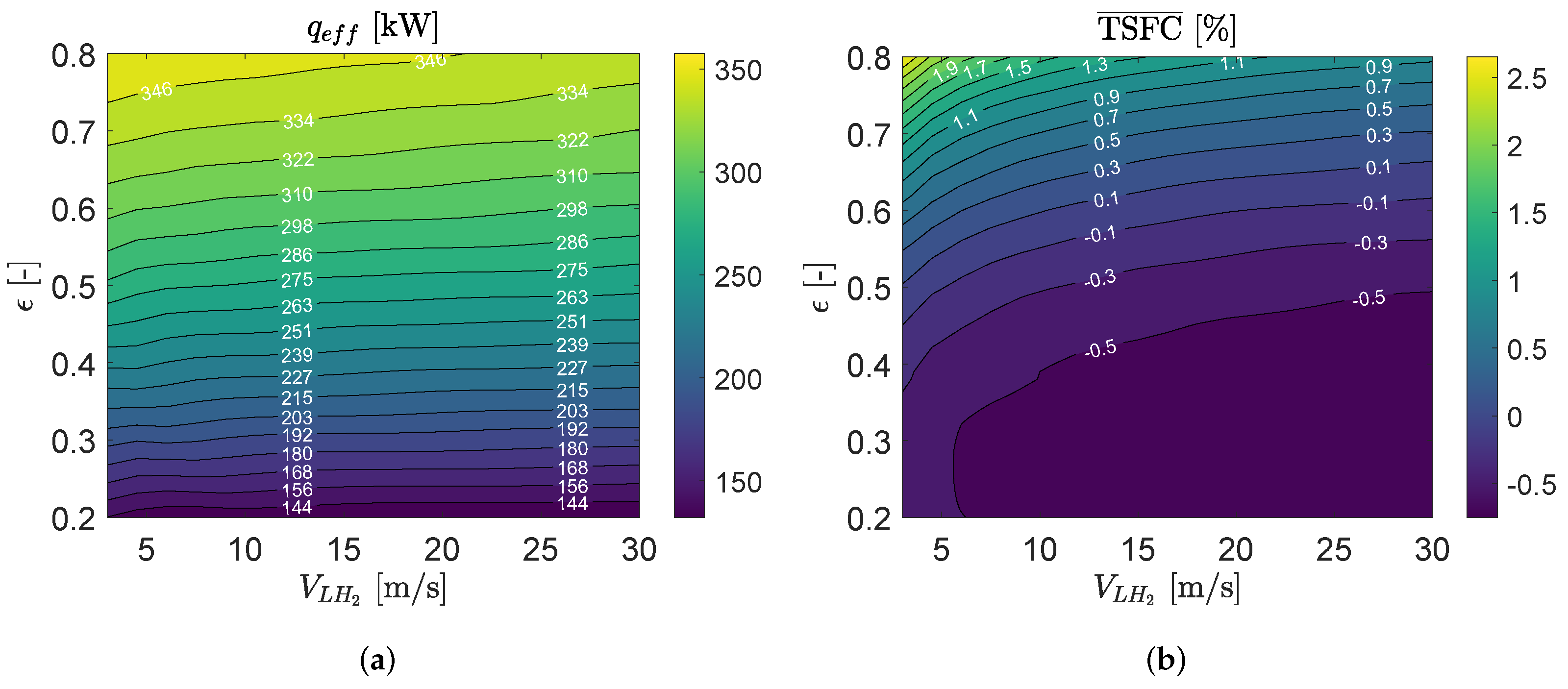
3.2. Parametric Study

The aerothermal impact of effectiveness and internal flow velocity on heat-exchanger sizing and performance are quantified in the present parametric study. It is assumed that the HE effectiveness at the design point varies between 0.2 and 0.8 while the velocity at the inlet of HE tubes at the design point is bounded in the range 3.0–30.0 [m/s]. Moreover, in this paper, a staggered tube bank configuration, as seen in Figure 6, is used as a generic model while the physical properties are scaled on the basis of the tube diameter. The wall thickness of HE tubes is computed based on the assumption of a constant ratio of inner and outer tube diameters equal to 0.65, i.e., $D_i/D_o=0.65$. The main focus is directed towards the net benefit by precooling and intercooling because the potential for re-optimizing the cycle for this type of heat sink is greater; however, due to the lower temperature of the compressor air, maximum benefits can only be achieved by combining an optimized compression system with a higher temperature source such as cooled cooling or core exhaust heat for fuel pre-heating ahead of the combustor.

In addition to the impact of the heat exchanger locations on the overall efficiency of the cycle, calculation of size, weight, and performance of the individual heat exchanger is a key task when designing the hydrogen-fueled propulsion system. To assess their individual impact on the performance of the engine’s cycle, numerical simulations were performed for the adapted LH₂ engine’s cycle, while in all cases the net thrust ($F_N$), design $FPR$, design $OPR$, and design $TIT$ are kept constant. Figure 7 shows the geometrical properties of the precooler and intercooler at different effectiveness and inner hydrogen flow velocities at the design point. To calculate the HE weight, it is assumed that the tubes are made of stainless steel type 316L with the density of 8000 [kg/m³]. Moreover, the HE weight ratio is computed by the weight of the heat exchanger normalized by a single point (associated with HE effectiveness of $ϵ=0.6$ and hydrogen velocity of $V_{L{H}_2}=15$ [m/s]).

In order to achieve a higher HE effectiveness, more surface area (expressed by NTU) is required, which is consistent with Equation (20).

The precooler is located in the annulus area between the fan and IPC. The frontal area ($A_{ft}$) of the chosen design with the staggered tube configuration is computed based on the core inlet stagnation properties and prescribed Mach number, which is assumed to be 0.12 in this study. The available frontal area, $A_{fr}$, to install the intercooler between the IPC and HPC is estimated in the same way and assuming the same Mach number. To achieve the required effectiveness, a relatively large number of tubes is required. In addition, the staggered tubular design results in small tube diameters ranging from 0.1 to 2.0 [mm]. A very small tube diameter indicates an impractical design resulting in high air-side pressure loss and risk of foreign object impact damage to the small tubes. The pressure loss over the increased diameter tubes is expected to increase, but the mass averaged total pressure loss should be similar to the case where the full annulus is used; however, in a compression system, such design seems impractical due to the need to mix the flow downstream of the heat exchanger at different pressures. Note that, for this study, a staggered tube configuration with a high solidity has been selected for the heat exchanger. Although impractical for the present application, it may give an indication of the design space exploration for the compact heat exchanger solutions for hydrogen-fueled gas turbine engines. Other types of heat exchangers are indeed believed to provide a practical compromise between tube diameter and heat transfer rate, such as more sparse tubular configuration including fins [24]. Another alternative is to use the existing turbomachinery surfaces (vanes, hub, and shroud surfaces) to benefit from high heat-transfer rates; however, the existing area might prove to be insufficient, requiring the extension of existing surfaces and increased pressure loss.

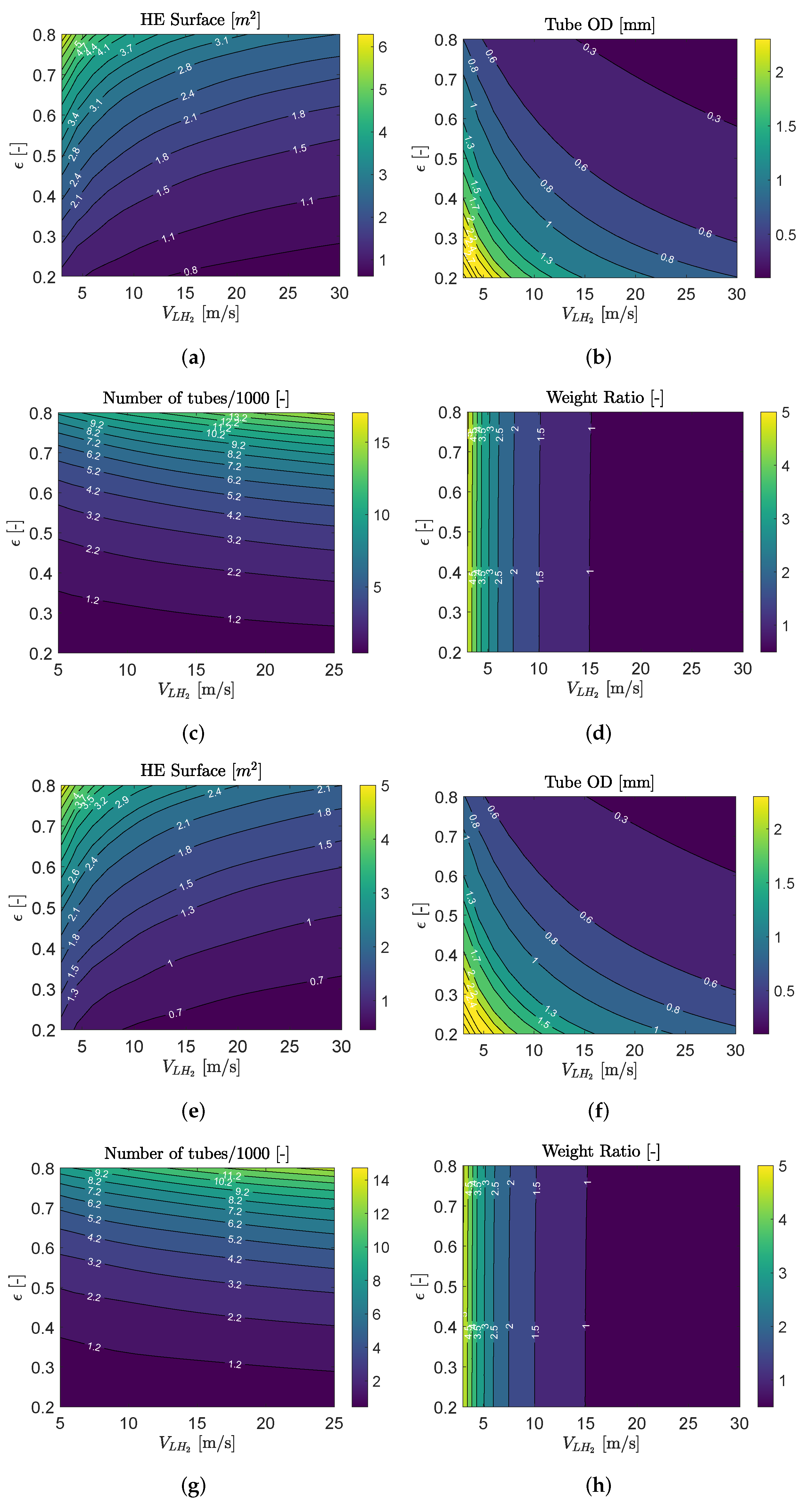
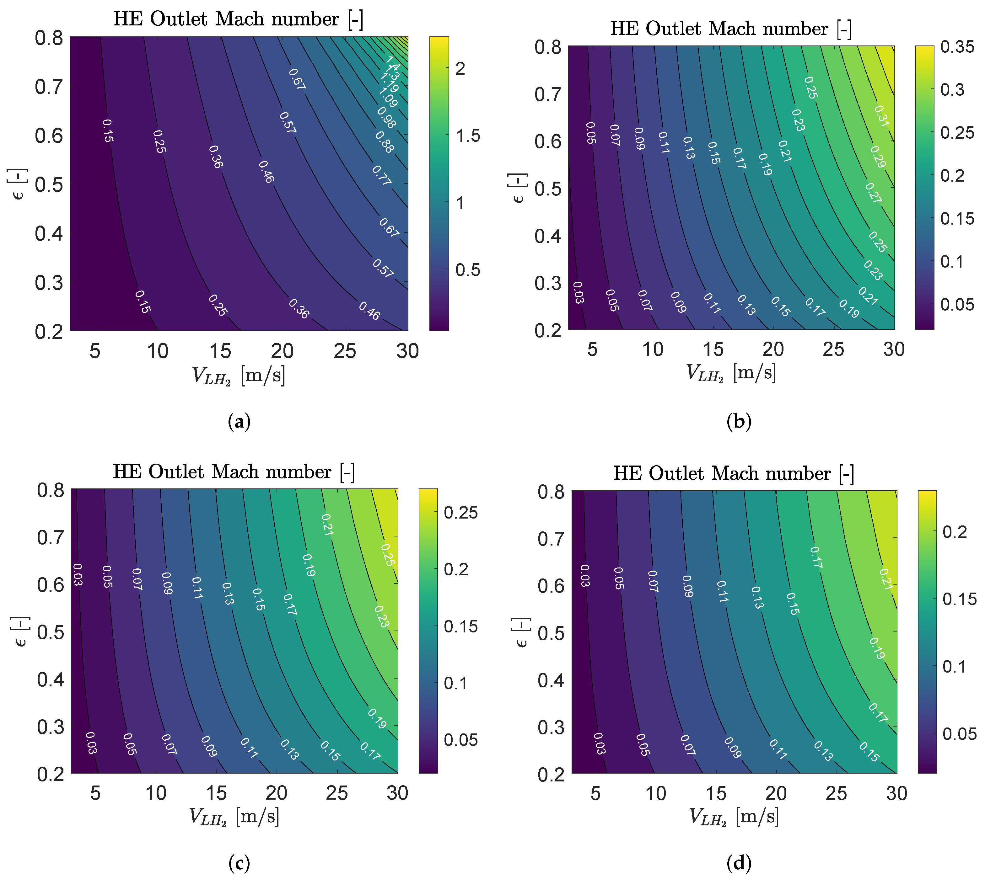
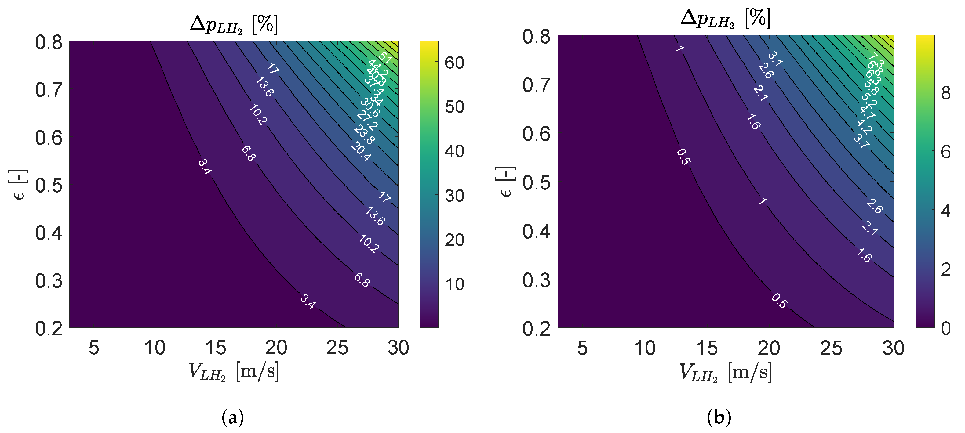
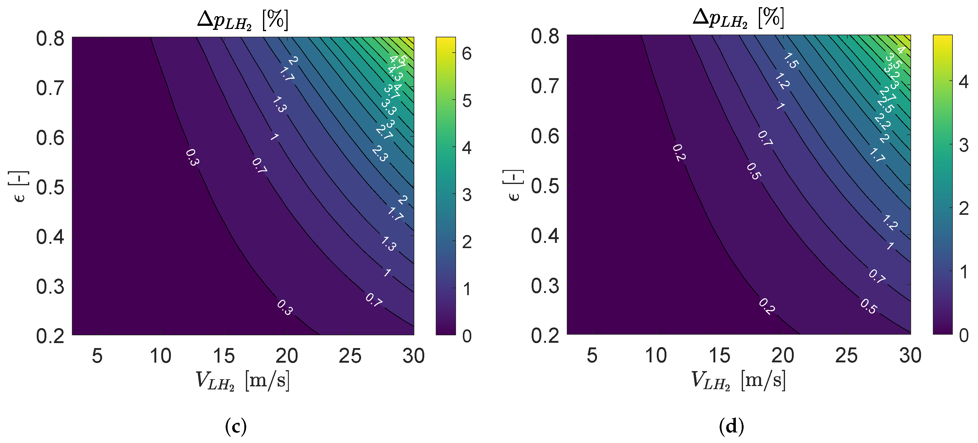
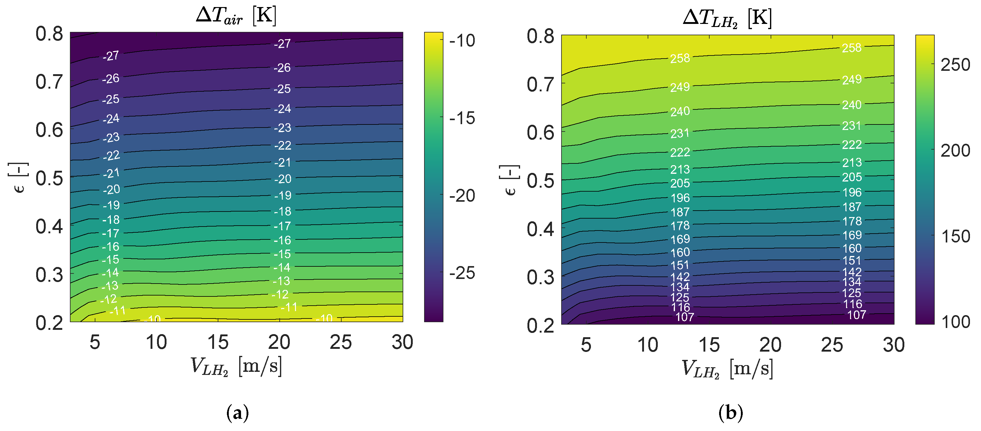
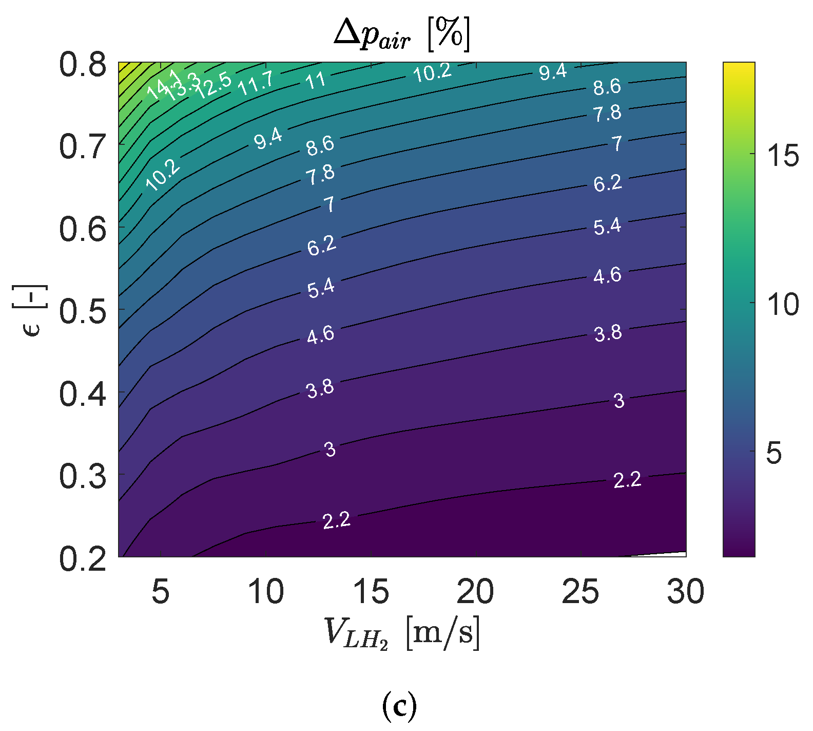
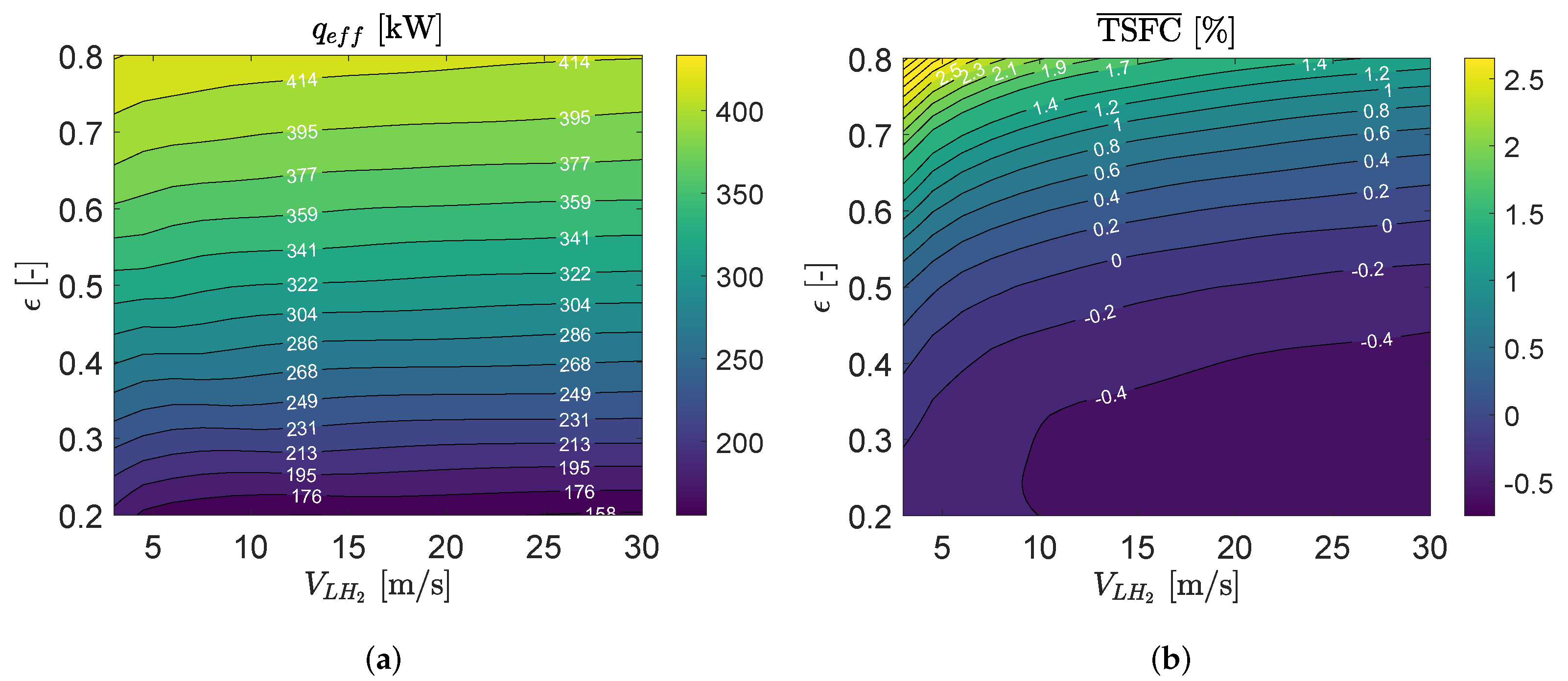
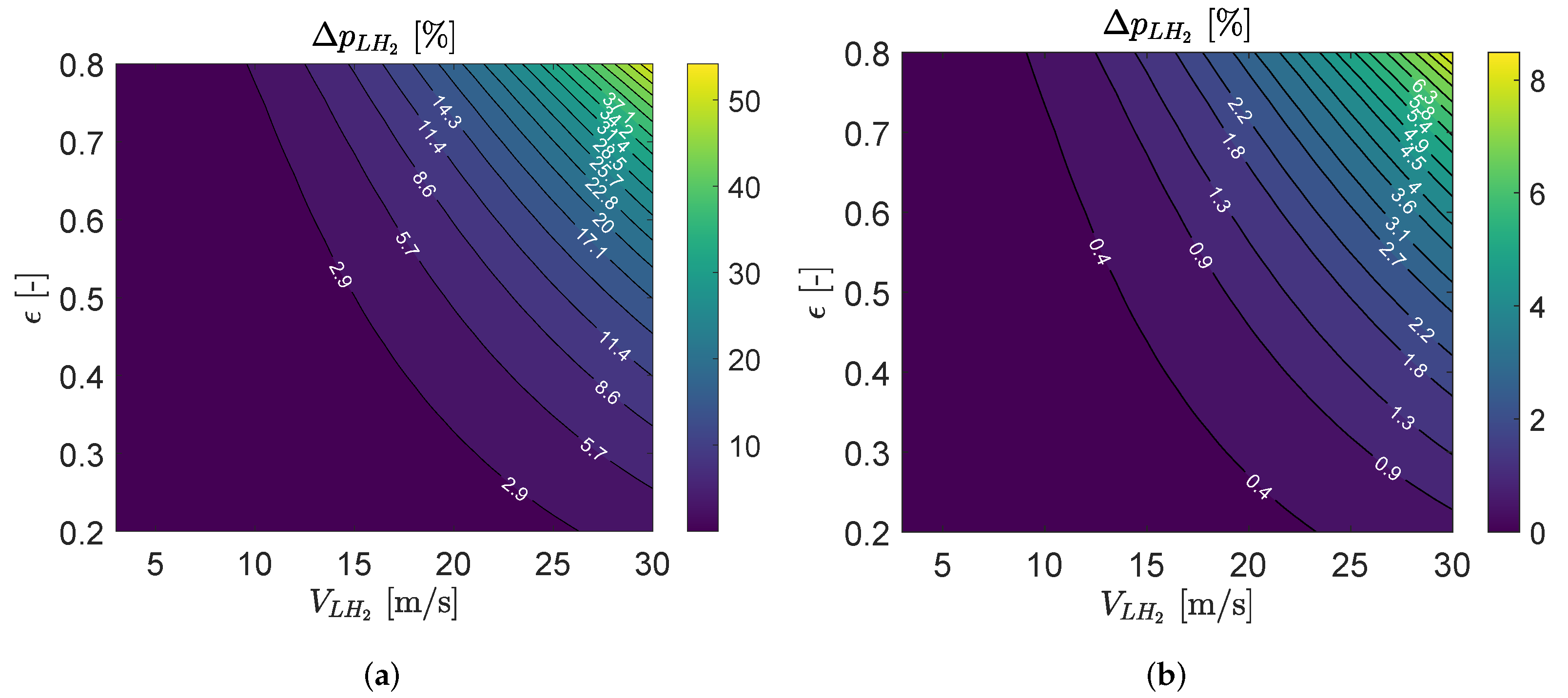
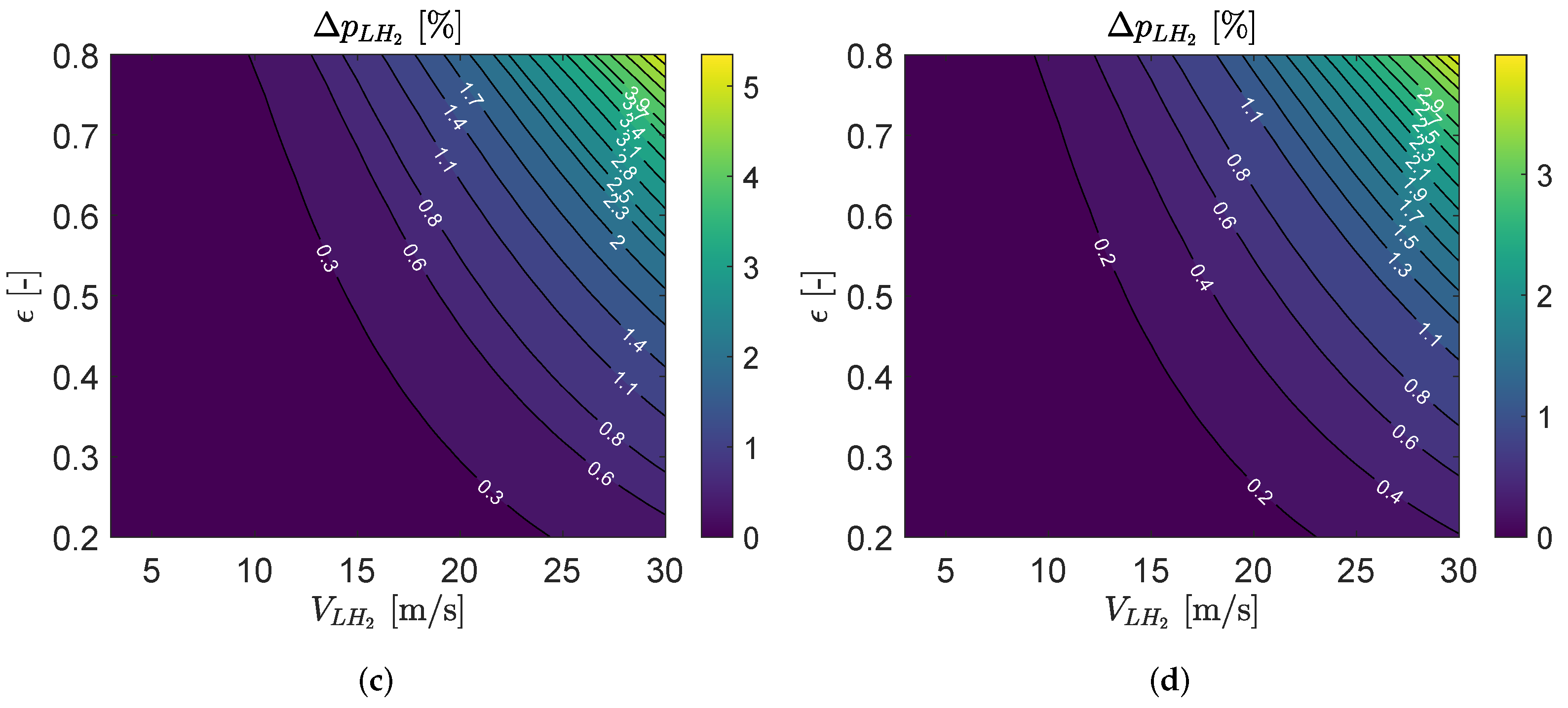
3.3. Precooler HE Performance

The impact of higher effectiveness, obtained by a larger surface area, on air and $H_2$ temperature differences across the precooler, is clearly seen in Figure 8a,b, where $\mathsf{\Delta }{T}_{air}=T_{air,out}-T_{air,in}$ and $\mathsf{\Delta }{T}_{H_2}=T_{H_2,out}-T_{H_2,in}$ are given. As expected, higher effectiveness provides more heating for $H_2$ and more cooling for the air; however, it undesirably increases the pressure drop for the air side because of a relatively large number of tubes (see Figure 8c). An air pressure drop of about 4–14% occurs for an effectiveness greater than 0.5 at the design point associated with the take-off operating condition as seen from Figure 8c. In addition, Figure 8a,b show that the temperature differences across the precooler, for both air and $H_2$, are proportional to the HE effectiveness, but mostly independent of the $H_2$ velocity inside the tubes. It can be also observed from Figure 7a that, by lowering the internal flow velocity, the required HE surface area increases, which leads to increasing air-side pressure drop ratios as shown in Figure 8c.

The amount of heat added to the fuel at the end of cruise by means of precooling can be seen in Figure 9a. For a given effectiveness at the design condition, a higher flow velocity inside the tubes slightly increases the heat transfer rate. Figure 9b provides the variation of installed $\mathrm{TSFC}$ at the end of cruise relative to the optimized LH₂ engine cycle. As illustrated, the precooler can improve the overall performance of the engine’s cycle at the end of the cruise operating condition; however, for a prescribed effectiveness above 60% at the design point associated with the take-off operating condition, it has no significant impact on the overall performance of the engine due to excessive pressure losses that are not outweighed by the increased fuel temperature. It is noted that the engine was not re-optimized for operation with a precooler. At low velocity flow at the inlet of the HE tubes and high prescribed effectiveness at the design point, the excessive pressure losses are also likely to deny any benefits arising from a cycle optimization, recalling that for each 1% loss in air pressure, there would be approximately 0.3% loss in SFC.

Figure 10 shows the Mach number of H₂ at the precooler HE outlet at four different operating conditions for varying effectiveness and flow velocity (at the inlet of the HE tubes) at the design point. Since the velocity of the hydrogen exiting the HEs is much higher than the entry velocity, the choking flow problem, associated with a higher inlet velocity or a lower working pressure relative to the hydrogen critical pressure, may occur. Hence, a very large prescribed HE effectiveness and inlet velocity at the design point are not feasible.

In addition, an undesirable impact of a higher prescribed HE effectiveness and inlet velocity at the design point on pressure drop of H₂ at the precooler outlet can be observed in Figure 11. Similar to the air pressure drop, for an effectiveness greater than 0.5 at the design point associated with the take-off operating condition, a pressure drop of about 0.2–4% occurs for the H₂ flow.

3.4. Intercooler HE Performance

Figure 12 shows the performance of the intercooler for various ranges of effectiveness and flow velocity at inlet of the HE tubes at the design point associated with the take-off operating condition. Similar to the precooler, a higher effectiveness yielding a larger surface area gives larger temperature changes across the intercooler on both air and $H_2$ sides as demonstrated in Figure 12a,b; however, it increases the air pressure drop (see Figure 12c). For the low velocity flow inside the tubes, higher effectiveness of the intercooler causes the air-pressure-drop ratio to be higher than in the precooler, but the pressure drop ratio for the internal flow is almost identical. Similar to in the precooler, the temperature difference is independent of the flow velocity at inlet of the HE tubes with respect to the effectiveness across the intercooler, as seen in Figure 12a,b; however, the temperature difference across the intercooler for both internal and external flows is 17–22% higher than that of the precooler, relating to the higher IPC delivery air density for the same effectiveness.

Figure 13a displays the rejected heat by the intercooler, which is added to the fuel. Compared with the precooler, the intercooler can supply 19–22% more heat to the fuel at the end-of-cruise condition for a given HE effectiveness at the design condition. Figure 13b presents the variation of installed TSFC relative to the optimized LH₂ engine cycle without HE. Comparing with the precooler, the intercooler does not reveal the more positive impact on the engine performance for a broad range of HE effectiveness levels. In this paper, the improvement in $\overline{\mathrm{TSFC}}$ is limited up to 0.3% for the prescribed HE effectiveness at the design condition between 0.5 and 0.6; however, by optimizing the engine’s cycle with a prescribed intercooler HE, a greater reduction in $\overline{\mathrm{TSFC}}$ is to be expected.

The Mach number of H₂ at the intercooler HE outlet at four different operating conditions for varying effectiveness and flow velocity (at the inlet of the HE tubes) at the design point is presented in Figure 14. The similar choking flow trouble in the precooler can be seen in the intercooler, giving rise to avoid an impractical prescription of a very large effectiveness and inlet velocity at the design point.

Furthermore, a higher prescribed HE effectiveness and inlet velocity at the design point increase the pressure drop of H₂ at the intercooler outlet as shown in Figure 15. As seen, the higher prescribed inlet velocity has a greater impact on the severe pressure drop of H₂ than the higher prescribed HE effectiveness.

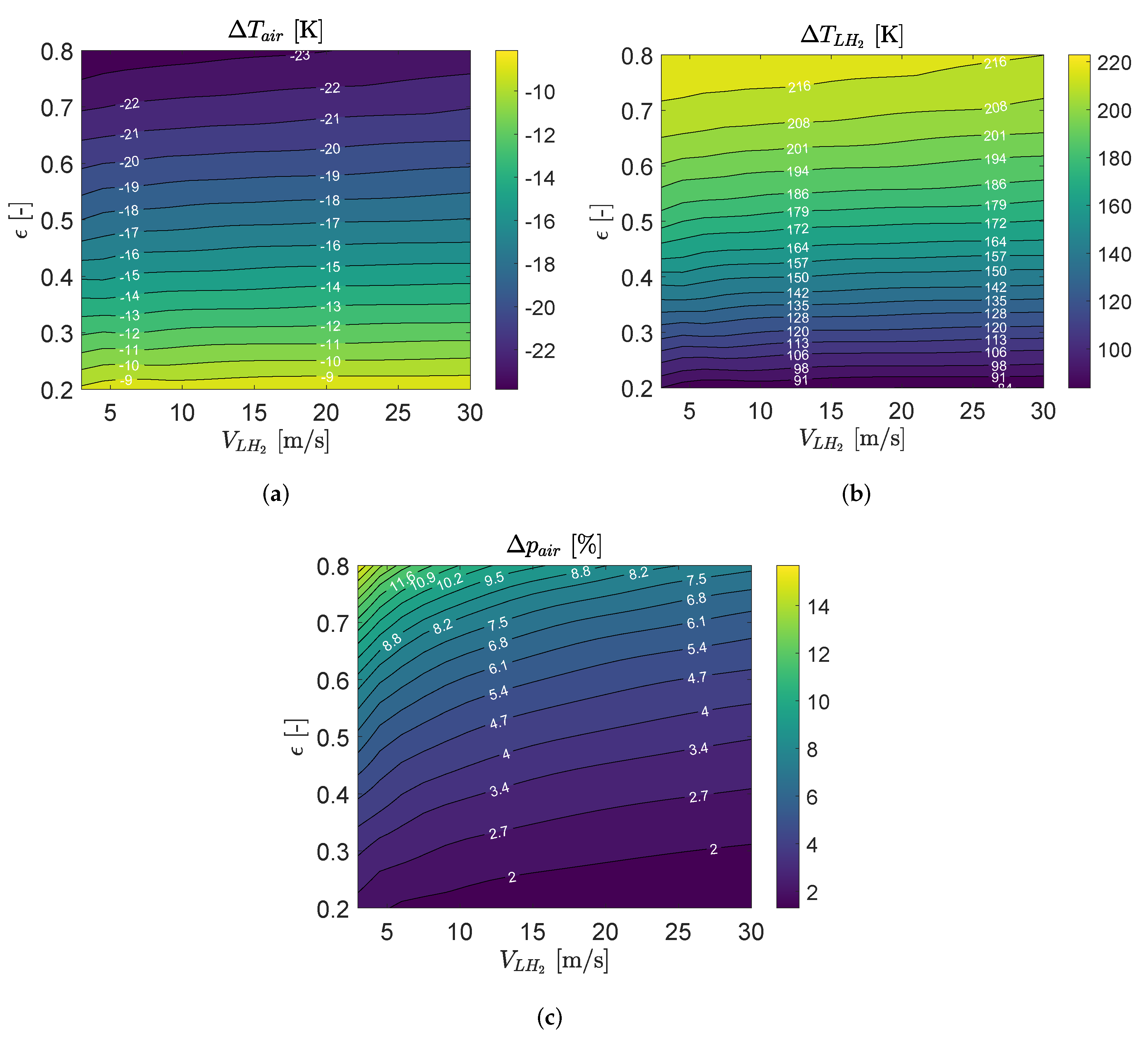
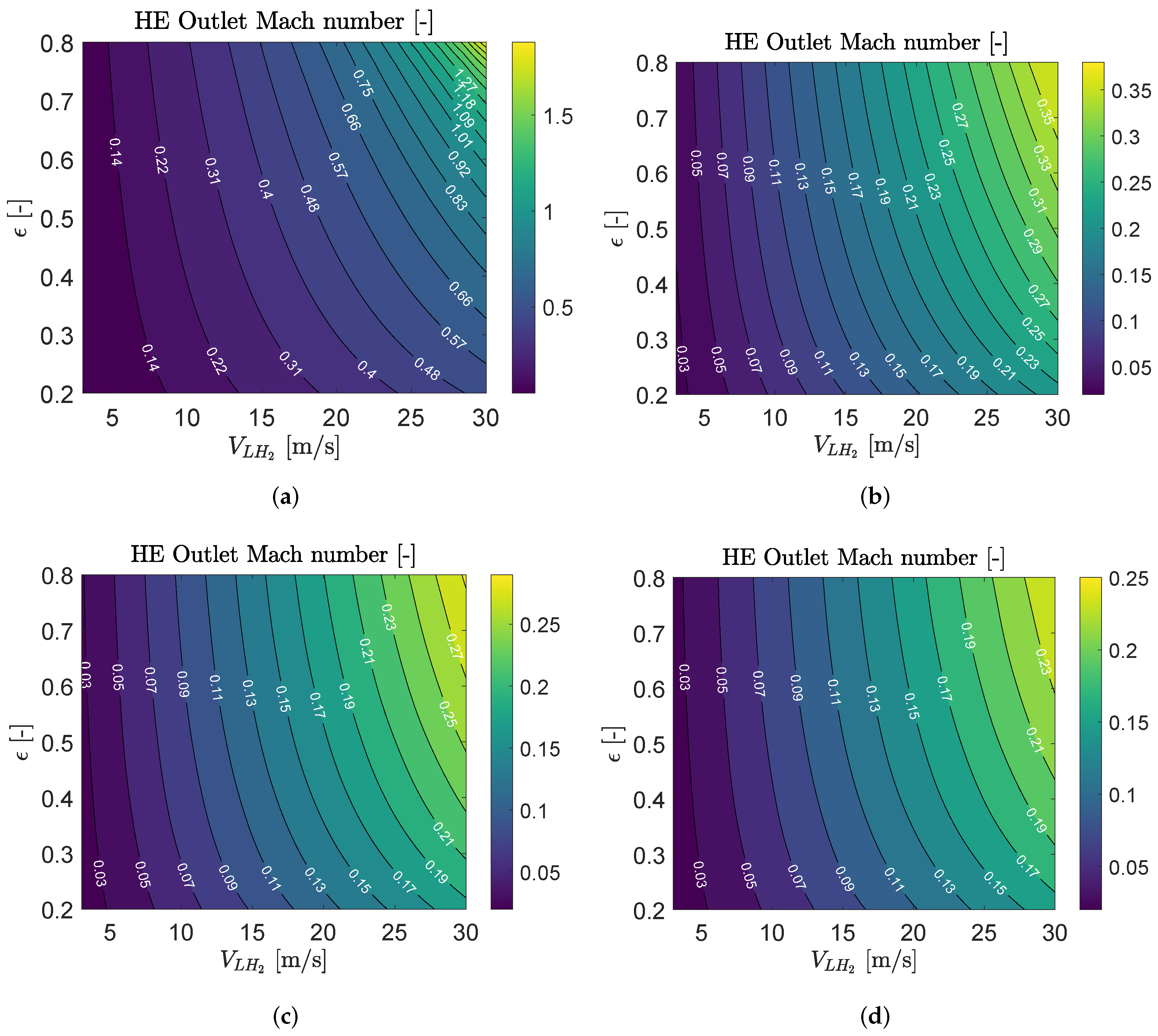
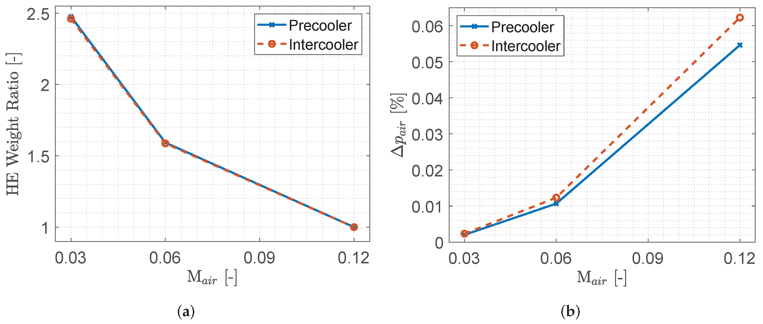
4. Sensitivity Analysis of External Flow Mach Number on Precooler and Intercooler

The previous results are based on the prescribed air flow Mach number of 0.12 (standard case). To study the effect of the prescribed air flow Mach number, additional simulations for two different Mach numbers, i.e., M${}_{air}=0.03$ (case 1) and M${}_{air}=0.06$ (case 2) were performed. This range was selected to create a reasonable pressure drop on the external side. Note that the pressure drop for an external Mach number of 0.12 ranges between 6% to 15% for an heat exchanger effectiveness between 60% and 80%, respectively. The sensitivity analysis is carried out for HE weight ratio (with respect to the standard case) and air pressure drop percentage across the HE tubes. Because of the similar trends in the results for varying HE effectiveness and hydrogen velocity at the inlet of the HE tubes, the results are presented for a single point associated with HE effectiveness of $ϵ=0.6$ and HE inlet velocity of $V_{L{H}_2}=15$ [m/s].

Figure 16 compares the impact of the prescribed air flow Mach number on the weight ratio of HE and air-side pressure drop percentage for both precooler and intercooler at the end-of-cruise condition for a prescribed HE effectiveness of $ϵ=0.6$ and HE inlet velocity of $V_{L{H}_2}=15$ [m/s] at the design point. As seen, the reduction in the prescribed airflow Mach number increases the weight ratio of both precooler and intercooler by a factor of ∼2.5 and ∼1.5 for the case 1 and case 2, respectively. This is because of the longer HE tubes as a result of the expansion of the frontal area for the lower prescribed external flow Mach number at the inlet of the heat exchanger (see Equation (24)). In addition, the reduction in the prescribed airflow Mach number (resulting in the lower core air velocity) decreases the air-side pressure loss percentage across the HE tubes by a factor of ∼0.04 and ∼0.20 for the case 1 and case 2, respectively.

5. Conclusions

A numerical framework to model hydrogen-fueled gas turbine engines with a dedicated heat-management system has been developed. The study has endeavored to provide a detailed description of the procedure to model such gas turbines with dedicated heat-management systems. The required tools and methods in this framework have been presented and discussed. Furthermore, the methods have been employed to analyze the impact of using LH₂ to precool and intercool in the compression system. The staggered-tube compact heat exchanger, chosen as the conceptual model of the heat exchanger (as shown in Figure 6), does not offer the lowest air-side pressure losses. Profiled tubes and different arrangements can approximately halve the loss, but are likely to be heavier. A more complex, but potentially better alternative, could be to use several stator rows with sparred hollow vanes, where fewer guide vanes are required for both the precooler and the intercooler. Nevertheless, a multistage configuration would be needed also for this design. The precooler hardly improves the overall performance of the engine’s cycle in the design condition. Regardless of a higher air pressure drop occurring at high HE effectiveness in the end-of-cruise condition, the precooler has a positive impact on the overall performance of the engine. Additionally, the problem of the icing-up of the vanes if the incoming air is at all humid may lead to the conclusion that precooling is not worth further study. The positive impact of the intercooler for a broad range of HE effectiveness can be observed. In this study, the improvement in $\mathsf{\Delta }\overline{\mathrm{TSFC}}$ is limited up to 0.3% for the HE effectiveness between 0.5 and 0.6; however, by optimizing the engine’s cycle with a prescribed intercooler, a greater reduction in $\overline{\mathrm{TSFC}}$ is expected. For a working pressure above the hydrogen critical pressure, since the hydrogen velocity at the outlet of both precooler and intercooler is much higher than the entry velocity, the choking flow problem may occur; therefore, a very large prescribed HE effectiveness and inlet velocity at the design point must be avoided. Finally, a reduction in external air flow Mach number, leading to decreases in the air-side pressure drop across the heat exchanger, can be penalized by increasing the weight of the heat exchanger.

References

1. Liu, Y.; Sun, X.; Sethi, V.; Nalianda, D.; Li, Y.G.; Wang, L. Review of modern low emissions combustion technologies for aero gas turbine engines. Prog. Aerosp. Sci. 2017, 94, 12–45. [Google Scholar] [CrossRef] [Green Version]
2. Rao, A.G.; Yin, F.; Werij, H.G. Energy Transition in Aviation: The Role of Cryogenic Fuels. Aerospace 2020, 7, 181. [Google Scholar] [CrossRef]
3. Grewe, V.; Gangoli Rao, A.; Grönstedt, T.; Xisto, C.; Linke, F.; Melkert, J.; Middel, J.; Ohlenforst, B.; Blakey, S.; Christie, S.; et al. Evaluating the climate impact of aviation emission scenarios towards the Paris agreement including COVID-19 effects. Nat. Commun. 2021, 12, 3841. [Google Scholar] [CrossRef] [PubMed]
4. Srinath, A.N.; Pena López, Á.; Miran Fashandi, S.A.; Lechat, S.; di Legge, G.; Nabavi, S.A.; Nikolaidis, T.; Jafari, S. Thermal Management System Architecture for Hydrogen-Powered Propulsion Technologies: Practices, Thematic Clusters, System Architectures, Future Challenges, and Opportunities. Energies 2022, 15, 304. [Google Scholar] [CrossRef]
5. Brewer, G.D. Hydrogen Aircraft Technology, 1st ed.; CRC Press: London, UK, 1991. [Google Scholar]
6. Westenberger, A. Hydrogen Fueled Aircraft. In Proceedings of the AIAA International Air and Space Symposium and Exposition: The Next 100 Years, Dayton, OH, USA, 14–17 July 2003. [Google Scholar] [CrossRef]
7. Jafari, S.; Nikolaidis, T. Thermal Management Systems for Civil Aircraft Engines: Review, Challenges and Exploring the Future. Appl. Sci. 2018, 8, 2044. [Google Scholar] [CrossRef] [Green Version]
8. Green, J.E. Greener by Design—The technology challenge. Aeronaut. J. 2002, 106, 57–113. [Google Scholar]
9. Verstraete, D. The Potential of Liquid Hydrogen for Long Range Aircraft Propulsion. Ph.D. Thesis, Cranfield University, Cranfield, UK, 2009. [Google Scholar]
10. Khandelwal, B.; Karakurt, A.; Sekaran, P.R.; Sethi, V.; Singh, R. Hydrogen powered aircraft: The future of air transport. Prog. Aerosp. Sci. 2013, 60, 45–59. [Google Scholar] [CrossRef]
11. Klug, H.G.; Faass, R. CRYOPLANE: Hydrogen fuelled aircraft—Status and challenges. Air Space Eur. 2001, 3, 252–254. [Google Scholar] [CrossRef]
12. Svensson, F.; Singh, R. Effects of Using Hydrogen on Aero Gas Turbine Pollutant Emissions, Performance and Design. In Proceedings of the Expo 2004, Turbo Expo: Power for Land, Sea, and Air, Vienna, Austria, 14–17 June 2004; Volume 2, pp. 107–116. [Google Scholar] [CrossRef]
13. Rogers, H.L.; Lee, D.S.; Raper, D.W.; Foster, P.M.D.F.; Wilson, C.W.; Newton, P.J. The impacts of aviation on the atmosphere. Aeronaut. J. 2002, 106, 521–546. [Google Scholar] [CrossRef]
14. Haglind, F.; Hasselrot, A.; Singh, R. Potential of reducing the environmental impact of aviation by using hydrogen Part I: Background, prospects and challenges. Aeronaut. J. 2006, 110, 533–540. [Google Scholar] [CrossRef]
15. Dahal, K.; Brynolf, S.; Xisto, C.; Hansson, J.; Grahn, M.; Grönstedt, T.; Lehtveer, M. Techno-economic review of alternative fuels and propulsion systems for the aviation sector. Renew. Sustain. Energy Rev. 2021, 151, 111564. [Google Scholar] [CrossRef]
16. Boggia, S.; Jackson, A. Some Unconventional Aero Gas Turbines Using Hydrogen Fuel. In Proceedings of the Turbo Expo 2002, Parts A and B, Turbo Expo: Power for Land, Sea, and Air, Amsterdam, The Netherlands, 3–6 June 2002; Volume 2, pp. 683–690. [Google Scholar] [CrossRef]
17. Dijk, I.; Gangoli Rao, A.; van Buijtenen, J. Stator cooling & hydrogen based cycle improvements. In Proceedings of the XIX International Symposium on Air Breating Engines (19th ISABE Conference), Montreal, ON, Canada, 7–11 September 2009; American Institute of Aeronautics and Astronautics Inc. (AIAA): Reston, VA, USA, 2009; pp. 1–10. [Google Scholar]
18. Grönstedt, T. Development of Methods for Analysis and Optimization of Complex Jet Engine Systems. Ph.D. Thesis, Chalmers University of Technology, Gothenburg, Sweden, 2000. [Google Scholar]
19. Pera, R.J.; Onat, E.; Klees, G.; Tjonneland, E. A Method to Estimate Weight and Dimensions of Aircraft Gas Turbine Engines; Report CR-159481; NASA: Washington, DC, USA, 1977. [Google Scholar]
20. Larsson, L.; Grönstedt, T.; Kyprianidis, K.G. Conceptual design and mission analysis for a geared turbofan and an open rotor configuration. In Proceedings of the ASME Turbo Expo: Turbomachinery Technical Conference and Exposition, Vancouver, BC, Canada, 6–10 June 2011. Number GT2011-46451. [Google Scholar] [CrossRef]
21. McBride, B.; Gordon, S. Computer Program for Calculating and Fitting Thermodynamic Functions; Report NASA RP-1271; NASA: Washington, DC, USA, 1992. [Google Scholar]
22. Lemmon, E.W.; McLinden, M.O.; Huber, M.L. NIST Standard Reference Database 23: Reference Fluid Thermodynamic and Transport Properties-REFPROP, Version 10.0; National Institute of Standards and Technology: Gaithersburg, MD, USA, 2018. [Google Scholar] [CrossRef]
23. White, F.M. Fluid Mechanics, 7th ed.; McGrawHill: New York, NY, USA, 2011. [Google Scholar]
24. Kays, W.; London, A. Compact Heat Exchangers; Krieger Pub. Co.: Malabar, FL, USA, 1984. [Google Scholar]
25. Timmerhaus, K.D.; Schoenhals, R.J. Design and Selection of Cryogenic Heat Exchangers Advances in Cryogenic Engineering. In Advances in Cryogenic Engineering; Springer: Boston, MA, USA, 1995; Volume 19, pp. 445–462. [Google Scholar] [CrossRef]
26. Incropera, F.P. Fundamentals of Heat and Mass Transfer; John Wiley & Sons, Inc.: Hoboken, NJ, USA, 2006. [Google Scholar]
27. Gnielinski, V. New Equations for Heat and Mass Transfer in Turbulent Pipe and Channel Flow. Int. Chem. Eng. 1976, 16, 359–368. [Google Scholar]
Figure 1. Cross-sectional meridional cut of a turbofan engine, including possible locations for core heat rejection to the hydrogen fuel. The fuel is stored at its boiling point in the cryogenic tank. The temperature of the hydrogen in the fuel line is increased by the different core-installed heat exchangers on its way to the combustion chamber. IPC: Intermediate-pressure compressor; HPC: High-pressure compressor; HPT: High-pressure turbine; LPT: Low-pressure turbine.
Aerospace 09 00216 g001
Figure 2. Temperature and FAR (fuel–air ratio) dependent tables for H2 combustion products at 1 bar. (a) Combustion exit temperature; (b) specific heat at constant pressure.
Aerospace 09 00216 g002
Figure 3. Variation of specific heat with respect to (a) temperature, and (b) pressure.
Aerospace 09 00216 g003
Figure 4. Schematic of cryogenic fuel distribution system connected to the structurally non-integrated tank.
Aerospace 09 00216 g004
Figure 5. Meridional view of compressor interconnecting duct featuring a compact hydrogen heat exchanger.
Aerospace 09 00216 g005
Figure 6. A generic staggered tube bank configuration (S 1.50–1.25a) for steady state flow [24].
Aerospace 09 00216 g006
Figure 7. HE surface area, tubes outside diameter, number of tubes, and weight ratio at the end-of-cruise condition for varying effectiveness and flow velocity at the inlet of the HE tubes at the design point: (ad) precooler, and (eh) intercooler.
Aerospace 09 00216 g007
Figure 8. Precooler HE performance parameters at the end-of-cruise condition: (a,b) temperature difference, and (c) pressure drop percentage across the HE tubes, for varying HE effectiveness and flow velocity at the inlet of the HE tubes at the design point.
Aerospace 09 00216 g008
Figure 9. Precooler HE, (a) effective heat transfer, and (b) relative TSFC ¯ for varying effectiveness and flow velocity at the inlet of the HE tubes at the design point.
Aerospace 09 00216 g009
Figure 10. Precooler HE performance parameter at the end-of-cruise condition Mach number of LH2 at the HE outlet for varying effectiveness and flow velocity at the inlet of the HE tubes at the design point. (a) Take-off, (b) top of climb, (c) initial cruise, and (d) end of cruise operating conditions.
Aerospace 09 00216 g010
Figure 11. Precooler HE, pressure drop of LH2 at the HE outlet for varying effectiveness and flow velocity at the inlet of the HE tubes at the design point. (a) Take-off, (b) top of climb, (c) initial cruise, and (d) end of cruise operating conditions.
Aerospace 09 00216 g011aAerospace 09 00216 g011b
Figure 12. Intercooler HE performance parameters at the end-of-cruise condition: (a,b) temperature difference, and (c) pressure drop percentage across the HE tubes, for varying HE effectiveness and flow velocity at the inlet of the HE tubes at the design point.
Aerospace 09 00216 g012aAerospace 09 00216 g012b
Figure 13. Intercooler HE, (a) effective heat transfer, and (b) TSFC ¯ for varying HE effectiveness and flow velocity at the inlet of the HE tubes at the design point.
Aerospace 09 00216 g013
Figure 14. Intercooler HE, Mach number of LH2 at the HE outlet for varying effectiveness and flow velocity at the inlet of the HE tubes at the design point. (a) Take-off, (b) top of climb, (c) initial cruise, and (d) end of cruise operating conditions.
Aerospace 09 00216 g014
Figure 15. Intercooler HE, pressure drop of LH2 at the HE outlet for varying effectiveness and flow velocity at the inlet of the HE tubes at the design point. (a) Take-off, (b) top of climb, (c) initial cruise, and (d) end of cruise operating conditions.
Aerospace 09 00216 g015aAerospace 09 00216 g015b
Figure 16. Precooler and intercooler HE: (a) the weight ratio of HE, and (b) air-side pressure drop percentage across the HE tubes (associated with the effectiveness of ϵ = 0.6 and inlet velocity of V L H 2 = 150 [m/s] at the design point of HE) for varying air-side Mach number.
Aerospace 09 00216 g016