Joint State and Parameter Estimation for Hypersonic Glide Vehicles Based on Moving Horizon Estimation via Carleman Linearization

Abstract

Aimed at joint state and parameter estimation problems in hypersonic glide vehicle defense, a novel moving horizon estimation algorithm via Carleman linearization is developed in this paper. First, the maneuver characteristic parameters that reflect the target maneuver law are extended into the state vector, and a dynamic tracking model applicable to various hypersonic glide vehicles is constructed. To improve the estimation accuracy, constraints such as path and parameter change amplitude constraints in flight are taken into account, and the estimation problem is transformed into a nonlinear constrained optimal estimation problem. Then, to solve the problem of high time cost for solving a nonlinear constrained optimal estimation problem, in the framework of moving horizon estimation, nonlinear constrained optimization problems are transformed into bilinear constrained optimization problems by linearizing the nonlinear system via Carleman linearization. For ensuring the consistency of the linearized system with the original nonlinear system, the linearized model is continuously updated as the window slides forward. Moreover, a CKF-based arrival cost update algorithm is also provided to improve the estimation accuracy. Simulation results demonstrate that the proposed joint state and parameter estimation algorithm greatly improves the estimation accuracy while reducing the time cost significantly.

1. Introduction

Due to their fast speed, high accuracy, long-range lethality, and unique survivability, hypersonic glide vehicles have brought great challenges to the modern defense system [1,2]. As one of the key technologies for hypersonic glide vehicle defense, the high-accuracy target tracking method has become a hot and difficult point of the study on antimissile technology in recent years [3,4]. However, only estimating the state is difficult to meet the requirements of target type recognition, maneuver mode recognition, and accurate trajectory prediction. To effectively defend hypersonic targets, it is necessary to accurately estimate their state and parameters.

Currently, the joint state and parameter estimation has attracted more and more attention, and some estimation algorithms have been developed and reported [4,5,6,7,8]. However, most current joint state and parameter estimation algorithms for hypersonic targets are designed in the framework of the Kalman filter system to improve the state estimation accuracy by constructing a more accurate parameter-augmented model, and pay little attention to the accuracy of parameter estimation. Due to the system state model’s strong nonlinearity, it is difficult for the Kalman filter algorithms based on model recursion to achieve accurate parameter estimation for hypersonic targets. Moreover, during flight, the vehicle is subjected to numerous constraints, the maneuver characteristic parameters change slowly, and their variation amplitudes are limited [9,10]. Taking various prior constraints into account in the estimator can help to improve the estimation accuracy, particularly parameter estimation accuracy. However, it is difficult for Kalman filter algorithms to consider prior inequality constraints. Therefore, the joint state and parameters estimation algorithm can consider numerous inequality constraints while improving estimation accuracy.

The essence of the estimation problem is to design an estimator, which can output the estimated system’s state according to the input measurement. Since the error characteristics are usually unknown, with the feedback correction idea of the control system for reference, the full information estimation algorithm based on the moving optimization principle of model predictive control (MPC) is proposed to improve estimation accuracy. However, the full information estimation algorithm suffers from the ‘data explosion’ problem [11]. By introducing the arrival cost, moving horizon estimation transforms the full information estimation problem into optimization problems within a sliding window and effectively solves the ‘data explosion’ problem. Moving horizon estimation, in contrast to traditional Kalman filters, introduces a feedback correction mechanism and realizes state estimation by solving a nonlinear optimization problem, significantly improving estimation accuracy. Unlike the traditional model-based recursive Kalman filters, the parameters in moving horizon estimation are independent optimization variables, which help to improve the parameter estimation accuracy, particularly for strongly nonlinear systems. Moving horizon estimation has been widely used in state estimation of nonlinear systems [12,13], such as UAVs [14], robotics [15], aircraft [16], etc., because of its high estimation accuracy and adaptability. Furthermore, by solving constrained optimization problems, state and parameter inequality constraints can be considered in moving horizon estimation to improve the estimation accuracy. Therefore, in this paper, moving horizon estimation is adopted to solve the joint state and parameter estimation problem in hypersonic glide vehicle defense.

However, due to the need to continuously solve the nonlinear optimization problems, the time cost of moving horizon estimation is usually quite high, especially when inequality constraints are considered. Adding inequality constraints will increase the time cost significantly. Therefore, the key to the engineering application of moving horizon estimation is reducing time costs while maintaining estimation accuracy. There are two primary ways for reducing the time cost. The first is to improve the solution algorithm of the nonlinear optimization problem to speed up the problem’s solution [17,18,19]. However, it is often difficult to improve optimization algorithms, and improved optimization algorithms are often less adaptive for nonlinear systems. Another way is to linearize the nonlinear system [20,21]. Combined with the characteristics of moving horizon estimation, the linearized model can maintain a high approximation accuracy by continuously updating the expansion points. The linearization methods have high adaptability and applicability. The most efficient way to reduce time costs is to linearize nonlinear systems. The Carleman linearization method was proposed by Torsten Carleman in 1932 and its core idea is: by changing a set of bases in the state space, the finite-dimensional nonlinear differential equations can be transformed into infinite-dimensional linear differential equations [22]. By Taylor expansion and augmenting new states that represent the higher order deviation terms to the original dynamic system state, the Carleman linearization method can accurately approximate the state equation of a nonlinear system [23]. Carleman linearization has attracted increasing attention and has been widely used in the linearization of nonlinear systems [24,25,26,27,28,29]. Therefore, in this paper, Carleman linearization is applied to the joint state and parameter estimation of the hypersonic target, and a moving horizon estimation algorithm via Carleman linearization is proposed to reduce time cost.

Moreover, arrival cost reflects the influence of historical data on state estimation, and its update accuracy has a direct impact on the accuracy and stability of system state estimation. However, for constrained linear or nonlinear systems, arrival cost usually does not have an analytical solution. Currently, the most common approach for updating the arrival cost is to approximate it with the estimated covariance matrix of the linear unconstrained system [30]. For constrained linear systems, the arrival cost update can be implemented using the standard Kalman filter or Kalman smoothing. For nonlinear systems, currently, there are mainly two approaches to updating the arrival cost: (1) Linearize the nonlinear system, use the EKF (extended Kalman filter) or convert the arrival cost update problem into a least-squares problem to solve [16,31]. The basic idea of EKF is to linearize the nonlinear system based on Taylor expansion and then use the Kalman filter to realize suboptimal estimation. However, due to the large error caused by the neglected high-order term in Taylor expansion, the estimation accuracy of the EKF algorithm for strongly nonlinear systems is usually low, and even filtering divergence occurs. (2) From the perspective of probability and statistics, the mean and covariance of state distribution are approximated by random or deterministic sampling [32,33], such as UKF (unscented Kalman filter), particle filter, etc. For strongly nonlinear systems, linearization methods often lead to large arrival cost update errors. Random or deterministic sampling filtering algorithms enable accurate mean and covariance predictions; thus, using the sampling filtering algorithm is beneficial to improve the accuracy of arrival cost update. Among the random or deterministic sampling filtering algorithms, CKF (Caubature Kalman filter) makes it possible to numerically compute multivariate moment integrals encountered in the nonlinear Bayesian filter based on the spherical–radial cubature rule and deterministic sampling. CKF is capable of accurately approximating the first two order statistical moments and has high applicability to high-dimensional nonlinear systems [34]. Furthermore, in the case of equal accuracy, the amount of calculation of the CKF algorithm is also less than that of other sampling filters, such as UKF and particle filter. Therefore, in this paper, CKF is adopted to update the arrival cost.

Motivated by the above discussions, the objective of this paper is to solve the joint state and parameter estimation problem in hypersonic glide vehicle defense. The contributions of this paper can be summarized as follows: A novel moving horizon estimation algorithm via Carleman linearization is developed. The maneuver characteristic parameters that reflect the target maneuver law are extended into the state vector, and a dynamic tracking model applicable to various hypersonic glide vehicles is constructed. To improve the estimation accuracy, the constraints in flight are taken into account, and the estimation problem is transformed into a constrained nonlinear optimal estimation problem. Then, to solve the problem of high time cost for solving nonlinear constrained optimal estimation problems, in the framework of moving horizon estimation, nonlinear constrained optimization problems are transformed into bilinear constrained optimization problems by linearizing the nonlinear system via Carleman linearization. For ensuring the consistency of the linearized system with the original nonlinear system, the linearized model is continuously updated as the window slides forward. The joint state and parameter accurate estimation is realized by solving the bilinear constrained optimization problem. Moreover, a CKF-based arrival cost update algorithm is also introduced to improve the estimation accuracy. Simulation results demonstrate that the proposed joint state and parameter estimation algorithm greatly improves the estimation accuracy while significantly reducing the time cost of tracking.

2. Problem Formulation

In this section, the maneuver characteristics are analyzed using the dynamics model, and the maneuver characteristic parameters that reflect the maneuver laws are extended into the state vector to construct an applicable dynamic tracking model that can be applied to various hypersonic glide vehicles. In flight, the vehicle is subject to numerous constraints, such as path constraints. Meanwhile, the maneuver characteristic parameters change slowly during flight, and their variation amplitudes are limited [9,10]. Therefore, to improve the estimation accuracy, the constraints and the variation amplitude of characteristic parameters in flight are considered, and the estimation problem is transformed into a nonlinear constrained optimal estimation problem.

2.1. System State Model

Hypersonic glide vehicle is mainly dominated by Earth’s gravity and aerodynamic force. The corresponding dynamics model is described as [35]:

$$\ddot{r}=\frac{\mathit{R}}{m}+\frac{G}{m}-{\mathit{\omega }}_e\times \left({\mathit{\omega }}_e\times r\right)-2{\mathit{\omega }}_e\times \dot{r}$$

(1)

where m is the mass of the vehicle, ω_e denotes the self-rotation angular rate of the Earth, and the gravitational G of the earth is determined by the position of the vehicle r.

$$\mathit{R}=-Di+L(j\sin \gamma +k\cos \mathit{\nu })$$

(2)

where L and D denote the aerodynamic lift and drag, respectively. ν is the bank angle. The traditional dynamic pressure model is used to describe the aerodynamic force [36]

$$D\approx \frac{1}{2}\rho v^{2}S{C}_D\left(\alpha ,Ma\right)$$

(3)

$$L\approx \frac{1}{2}\rho v^{2}S{C}_L\left(\alpha ,Ma\right)$$

(4)

where ρ represents atmospheric density, v is the vehicle velocity, and S is the reference area of the vehicle. C_L and C_D denote the aerodynamic coefficients, which are functions of the angle of attack α and Mach number Ma.

The vehicle’s maneuver is mainly determined by the characteristic parameters u_L, u_D, and γ. u_L and u_D are defined as:

$$\left\{\begin{array}{c}{u}_D=\frac{S{C}_D}{m}\\ u_L=\frac{S{C}_L}{m}\end{array}\right.$$

(5)

By extending the characteristic parameters into the state vector, the following joint state and parameter estimation model is constructed:

$$\left\{\begin{array}{l}\dot{r}=\mathit{v}\\ \dot{\mathit{v}}=C_{\mathit{v}}^P\left(\theta ,\sigma ,\gamma \right)\left[\begin{array}{l}-\frac{1}{2}\rho v^2{u}_D\\ \frac{1}{2}\rho v^2{u}_L\\ 0\end{array}\right]+g-2{\mathit{\omega }}_e\times \mathit{v}-{\mathit{\omega }}_e\times \left({\mathit{\omega }}_e\times r\right)\\ \left[\begin{array}{c}{\dot{u}}_D\\ {\dot{u}}_L\\ \dot{\gamma }\end{array}\right]=\left[\begin{array}{c}{w}_D\\ w_L\\ w_{\gamma }\end{array}\right]\end{array}\right.$$

(6)

where C_v^p(θ, σ, γ) is the conversion relationship between the velocity coordinate system and the radar coordinate system, state variable x = [r, v, u_D, u_L, γ], the sampling period is T, and w_D, w_L, and w_γ are Gaussian white noise.

In consideration of the detection system, the system state model can be described as:

$$\left\{\begin{array}{l}\dot{\mathit{x}}=f(\mathit{x})+w\hfill \\ y=h(\mathit{x})+\mathit{v}\hfill \end{array}\right.$$

(7)

where f(x) is the joint state and parameter estimation model shown in Equation (6), h(x) denotes the system measurement equation, w and v represent Gaussian white noises, and the covariances of system noise w and measurement noise v are Q and R, respectively.

2.2. Inequality Constraints

In flight, the vehicle is subjected to numerous constraints. Taking constraints into consideration in the estimator can help to improve the estimation accuracy. Generally, flight path constraints are the most commonly considered. There are three typical path constraints: the heating rate $\dot{Q}$, the dynamic pressure q, and the aerodynamic load n:

$$\dot{Q}=K_Q{\left(\frac{\rho }{{\rho }_0}\right)}^{0.5}{\left(\frac{v}{v_c}\right)}^{3.15}\le {\dot{Q}}_{\max }$$

(8)

$$q_{\min }\le q=\frac{1}{2}\rho v^2\le q_{\max }$$

(9)

$$n=q\sqrt{u_D{}^2+u_L{}^2}\frac{S}{mg}\le n_{\max }$$

(10)

where Equation (8) is the Kemp–Riddell formula, ρ₀ is the sea-level atmospheric density, v_c is the first cosmic velocity of the Earth, and K_Q is a constant.

During the flight, the maneuver characteristic parameters u_L, u_D change slowly, and their variation amplitudes are limited [9,10]. Therefore, the characteristic parameter constraints can be taken into account in the estimator:

$$u_D{}_{\min }\le u_D\le u_D{}_{\max }$$

(11)

$$u_L{}_{\min }\le u_L\le u_L{}_{\max }$$

(12)

Furthermore, with the continuous decrease in the vehicle’s speed, the maximum variation amplitude of the bank angle decreases gradually. The bank angle symbol can also be judged according to the vehicle’s turning direction:

$$0<\gamma \le {\left|\gamma (v)\right|}_{\max } \mathrm{or} -{\left|\gamma (v)\right|}_{\max }<\gamma \le 0$$

(13)

2.3. Nonlinear Constrained Optimal Estimation Problem

The essence of the estimation problem is to design an estimator that can output the estimated value ${\widehat{\mathit{x}}}_k$ of the system state x_k according to the input measurement at time k. The following requirement must be met by the estimator [11]:

$$e_k:={\mathit{x}}_k-{\widehat{\mathit{x}}}_k\to 0,k\to \infty ,$$

(14)

The inequality constraints cannot be considered in traditional Kalman filter algorithms based on model recurrence, and the character of the error e_k cannot be directly judged. Therefore, the feedback correction idea of the control system is used for reference, and the moving optimization principle of model predictive control (MPC) is adopted to design the estimator. Then, the estimation problem in Equation (7) is transformed into the following finite-time constrained optimization problem.

Problem 1

$${\Phi }_t^{*}:=\underset{{\mathit{x}}_0,{\left\{w_k\right\}}_{k=0}^{t-1}}{\min }{\Phi }_T^{}({\left\{w_k\right\}}_{k=0}^{t-1},{\mathit{x}}_0)$$

(15)

s.t.

Dynamic constraints: Equation (7).

Inequality constraints: Equations (8)–(13).

where ${\widehat{\mathit{x}}}_0$ is a priori estimated value of the system’s initial state and P₀⁻¹ is a symmetric positive definite weight matrix:

$${\Phi }_t^{}({\left\{w_k\right\}}_{k=0}^{t-1},{\mathit{x}}_0)={‖{\mathit{x}}_0-{\widehat{\mathit{x}}}_0‖}_{P_0^{-1}}^2+{\displaystyle \sum _{k=0}^{t-1}({‖{\mathit{v}}_k‖}_{{\mathit{R}}^{-1}}^2+{‖w_k‖}_{Q^{-1}}^2)}$$

(16)

where

$$\left\{\begin{array}{l}{‖{\mathit{v}}_k‖}_{{\mathit{R}}^{-1}}^2={\mathit{v}}_k{}^T{\mathit{R}}^{-1}{\mathit{v}}_k\\ {‖{\mathit{w}}_k‖}_{{\mathit{Q}}^{-1}}^2={\mathit{w}}_k{}^T{Q}^{-1}{\mathit{w}}_k\\ {‖{\mathit{x}}_0-{\widehat{\mathit{x}}}_0‖}_{P_0^{-1}}^2={({\mathit{x}}_0-{\widehat{\mathit{x}}}_0)}^T{P}_0^{-1}({\mathit{x}}_0-{\widehat{\mathit{x}}}_0)\end{array}\right.$$

(17)

$${\left\{w_k\right\}}_{k=0}^{t-1}:=\{w_0,w_1,\cdots ,w_{t-1}\}$$

(18)

Problem 1 is known as full information estimation because it utilizes all measured data to estimate the system state and disturbance. However, with the continuous increase in tracking time T, the amount of input measured data gradually increases, resulting in an increasing amount of calculation for solving optimization Problem 1. Especially, the amount of calculation and time cost will significantly increase when there are inequality constraints. When t → ∞, the input and amount of calculation will increase infinitely, resulting in a ‘data explosion’ and the inability to solve Problem 1. As a result, full information estimation is difficult to meet engineering application requirements, and moving horizon estimation has been proposed.

3. Moving Horizon Estimation Algorithm via Carleman Linearization

Although the moving horizon estimation algorithm effectively solves the ‘data explosion’ problem of full information estimation, its time cost is still high due to the need to continuously solve the nonlinear optimization problem, especially when inequality constraints are taken into account. Adding inequality constraints will increase the time cost significantly. To solve the problem of high time cost for solving the nonlinear constrained optimal estimation problem, Carleman linearization is utilized in this section to transform the nonlinear constrained optimal estimation problem into a bilinear constrained optimal estimation problem. The linearization model is continuously updated in the framework of moving horizon estimation to ensure the consistency of the bilinear system with the original nonlinear system. The joint state and parameter accurate estimation is realized through solving the bilinear constrained optimization problem.

3.1. Moving Horizon Estimation Principle

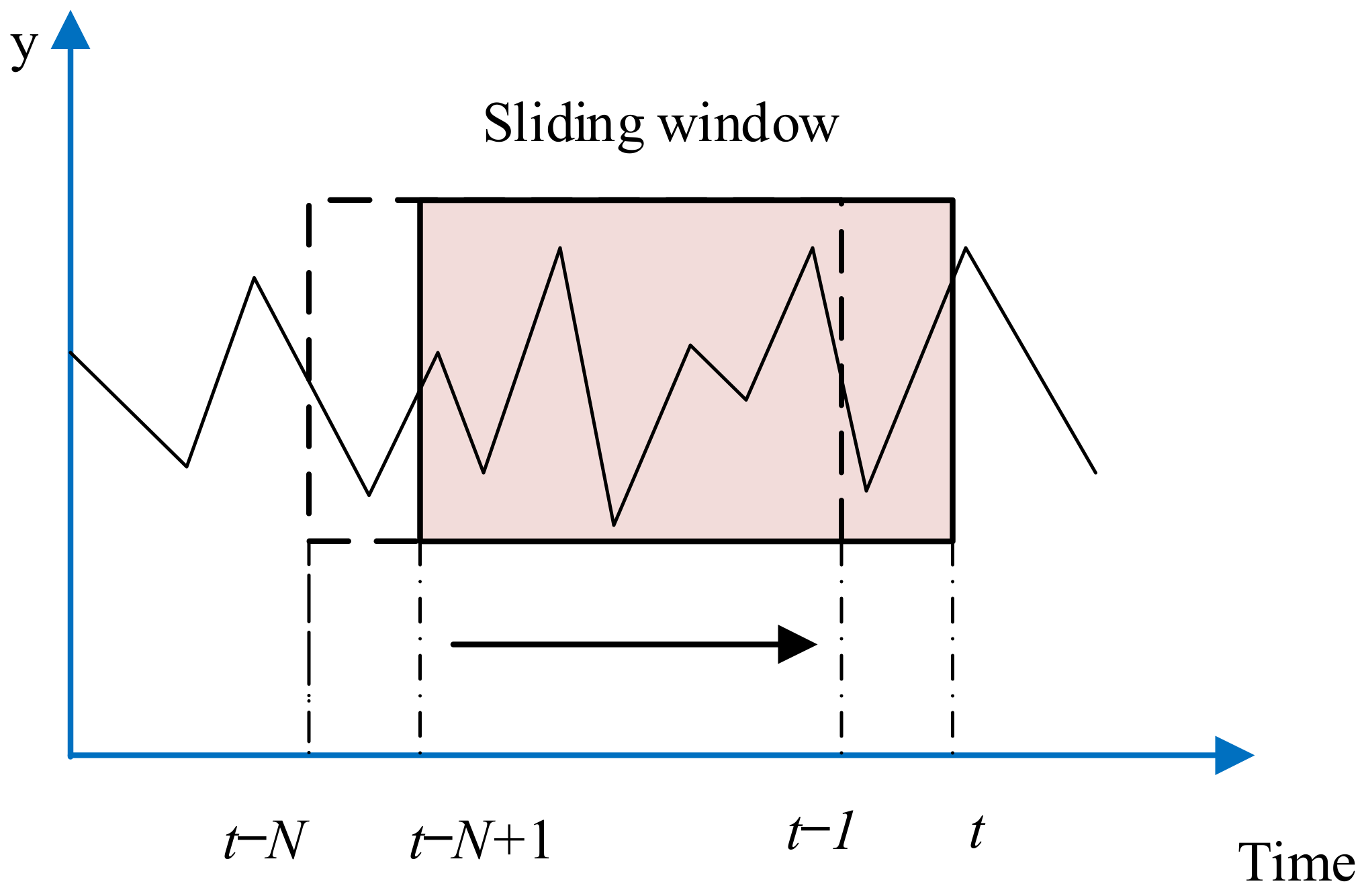
For avoiding the ‘data explosion’ problem of full information estimation and reducing the time cost, the measured data sequence is divided into historical data {0 ≤ k ≤ t − N − 1} and window data {t − N ≤ k ≤ t − 1} by introducing a sliding window with a data length of N as shown in Figure 1. Then, Equation (16) can be rewritten as:

$$\begin{array}{cc}\hfill & {\Phi }_t({\left\{{\mathit{w}}_k\right\}}_{k=0}^{t-1},{\mathit{x}}_0)={∥{\mathit{x}}_0-{\widehat{\mathit{x}}}_0∥}_{P_0^{-1}}^2+\sum _{k=0}^{t-1}({∥{\mathit{v}}_k∥}_{{\mathit{R}}^{-1}}^2+{∥{\mathit{w}}_k∥}_{Q^{-1}}^2)\hfill \\ \hfill & \begin{array}{cccc}& & & \end{array}\begin{array}{c}\hfill \end{array}\begin{array}{c}\begin{array}{c}\hfill \end{array}\hfill \end{array}\begin{array}{c}\hfill \end{array}={∥{\mathit{x}}_0-{\widehat{\mathit{x}}}_0∥}_{P_0^{-1}}^2+\sum _{k=0}^{t-N-1}{∥{\mathit{v}}_k∥}_{{\mathit{R}}^{-1}}^2+\sum _{k=0}^{t-N-1}{∥{\mathit{w}}_k∥}_{Q^{-1}}^2+\hfill \\ \hfill & \begin{array}{cccc}& & & \end{array}\begin{array}{c}\hfill \end{array}\begin{array}{c}\begin{array}{c}\hfill \end{array}\hfill \end{array}\begin{array}{c}\hfill \end{array}\begin{array}{c}\begin{array}{c}\hfill \end{array}\hfill \end{array}\begin{array}{c}\hfill \end{array}\sum _{k=t-N}^{t-1}{∥{\mathit{v}}_k∥}_{{\mathit{R}}^{-1}}^2+\sum _{k=t-N}^{t-1}{∥{\mathit{w}}_k∥}_{Q^{-1}}^2\hfill \\ \hfill & \begin{array}{cccc}& & & \end{array}\begin{array}{c}\hfill \end{array}\begin{array}{c}\begin{array}{c}\hfill \end{array}\hfill \end{array}\begin{array}{c}\hfill \end{array}={\Phi }_{t-N}({\mathit{x}}_0,{\left\{{\mathit{w}}_k\right\}}_{k=0}^{T-N-1})+\sum _{k=t-N}^{t-1}{∥{\mathit{v}}_k∥}_{{\mathit{R}}^{-1}}^2+\sum _{k=t-N}^{t-1}{∥{\mathit{w}}_k∥}_{Q^{-1}}^2\hfill \end{array}$$

(19)

Since the system in Equation (7) has Markov characteristics, the last two terms on the right side of the above equation are only determined by the state ${\mathit{x}}_{t-N}$ at time t − N and the noise sequence ${\left\{{\mathit{w}}_k\right\}}_{t-N}^{t-1}$. According to the first term on the right side of Equation (19), the following constrained optimization problem is defined.

Problem 2

$${{\Theta }}_{\tau }(\chi ):=\underset{{\mathit{x}}_0,{\left\{w_k\right\}}_{k=0}^{\tau -1}}{\min }{\Phi }_{\tau }^{}({\left\{w_k\right\}}_{k=0}^{k=\tau -1},{\mathit{x}}_0)$$

(20)

s.t.

Dynamic constraints: Equation (7).

Inequality constraints: Equations (8)–(13).

The optimal value of Equation (20) is the first term on the right side of Equation (19), which represents the necessary condition for the system to transfer from the initial state ${\mathit{x}}_0$ to the state χ, which is called the arrival cost. Based on the forward dynamic programming principle, Problem 1 can be transformed into the following form.

Problem 3

$${\Phi }_t^{*}:=\underset{{\mathit{x}}_{t-N},{\left\{w_k\right\}}_{k=t-N}^{k=t-1}}{\min }{\Phi }_t^{}({\left\{w_k\right\}}_{k=t-N}^{k=t-1},{\mathit{x}}_{t-N})$$

(21)

s.t.

Dynamic constraints: Equation (7).

Inequality constraints: Equations (8)–(13)

where

$${\Phi }_t({\mathit{x}}_{t-N},{\left\{{\mathit{w}}_k\right\}}_{k=t-N}^{k=t-1})={\mathsf{\Theta }}_{t-N}({\mathit{x}}_{t-N})+{\displaystyle \sum _{k=t-N}^{t-1}{‖{\mathit{v}}_k‖}_{{\mathit{R}}^{-1}}^2+{\displaystyle \sum _{k=t-N}^{t-1}{‖{\mathit{w}}_k‖}_{Q^{-1}}^2}}$$

(22)

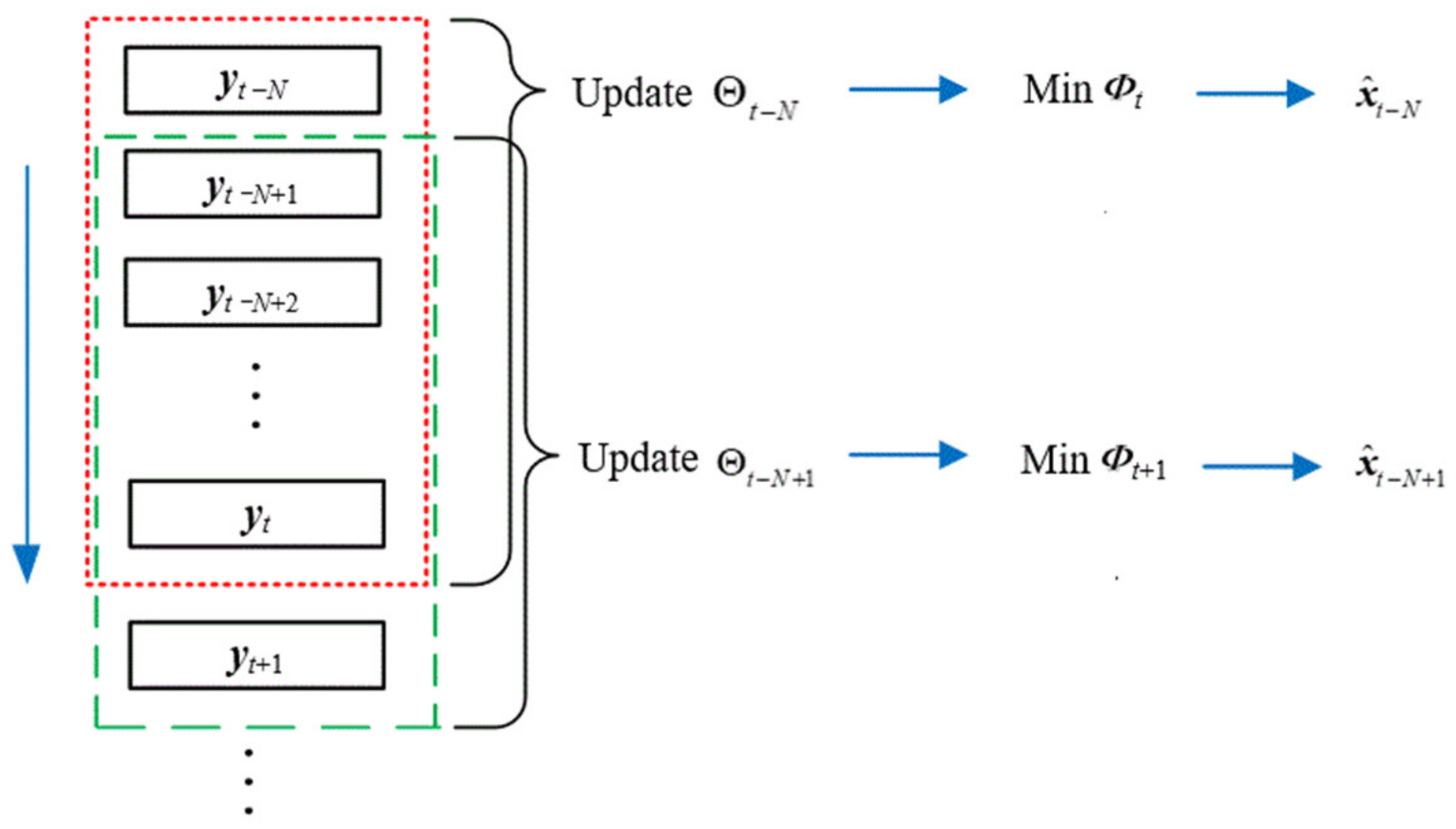
In the above equation, ${\mathsf{\Theta }}_{t-N}({\mathit{x}}_{t-N})$ is the arrival cost of state ${\mathit{x}}_{t-N}$, that is, the optimization value of Problem 2 at time t − N. The introduction of the arrival cost ensures the consistency between moving horizon estimation and full information estimation. The detailed steps of the moving horizon estimation are shown in Figure 2. When t ≤ N, the state estimation can be realized by solving the full information estimation problem (Problem 1). When t > N, first, the arrival cost ${\mathsf{\Theta }}_{t-N}({\mathit{x}}_{t-N})$ at time t is updated, and then the system state at time t − N is estimated by solving Problem 3. Then, the window slides forward; that is, the measured data at time t − N is discarded, and the measured data at time t + 1 is imported. When N = 1, the moving horizon estimation is equivalent to the Kalman filter for an unconstrained linear system.

3.2. Carleman Linearization

To facilitate the introduction of the Carleman linearization method, the following nonlinear dynamic systems is defined:

$$\dot{x}=f(x)$$

(23)

The nonlinear functions f(x) in Equation (23) is approximated at a specified point x₀ by Taylor expansion:

$$f(x)=f(x_0)+{\displaystyle \sum _{k=1}^{\eta }\frac{1}{k!}}{\left.\partial f_{[k]}\right|}_{x=x_0}{(x-x_0)}^{[k]}$$

(24)

where η denotes the expansion order, and x^[k] is the kth Kronecker product.

∂f_[k] is the kth partial derivative of f(x) at x = x₀ and can be calculated by:

$$\partial f_{[k]}=\left\{\begin{array}{ll}\frac{\partial f}{\partial \mathit{x}}\hfill & k=1\hfill \\ \frac{\partial }{\partial \mathit{x}}\otimes \partial f_{[k-1]}\hfill & k>1\hfill \end{array}\right.$$

(25)

To facilitate the derivation without loss of generality, it is assumed that the expansion point x₀ = 0. Thus, nonlinear dynamic systems in Equation (23) can be approximated by a polynomial form:

$$\begin{array}{l}\dot{x}\simeq A_0+A_1\mathit{x}+A_2{x}^2+\cdots +A_{\eta }{x}^{\eta }\\ \begin{array}{l}\hfill \end{array}\simeq {\displaystyle \sum _{k=0}^{\eta }{A}_k{x}^{[k]}}\end{array}$$

(26)

where

$$A_k={\left.\frac{1}{k!}\partial f_{[k]}\right|}_{\mathit{x}=0},A_0=f(0)$$

(27)

To realize Carleman linearization, the state vector of the system is extended to x_⊗:

$$x_{\otimes }={[x^T {(x^{[2]})}^T \cdots {(x^{[\eta ]})}^T]}^T$$

(28)

For verifying whether the extended state x_⊗ is consistent with the original state x, the higher-order term of the original state x is differentiated based on Equation (26). ${\dot{x}}^{[k]}$ is represented as:

$$\begin{array}{l}{\dot{x}}^{[k]}=x^{[k-1]}{\displaystyle \sum _{l=0}^{k-1}{I}_n^{[l]}\otimes \dot{x}\otimes }{I}_n^{[k-1-l]}\\ \begin{array}{l}\hfill \end{array}\begin{array}{l}\hfill \end{array} =x^{[k-1]}{\displaystyle \sum _{l=0}^{k-1}{I}_n^{[l]}\otimes ({\displaystyle \sum _{n=0}^{\eta }{A}_n{x}^{[n]}})\otimes }{I}_n^{[k-1-l]}\end{array}$$

(29)

It can be seen from the above equation that ${\dot{x}}^{[k]}$ is the function of the polynomials x^[k–1], x^[k],…, x^{[η + k–1]}, and the maximum order of the polynomials is η + k − 1. However, in the extended state, the highest order polynomial is x^[η]. Therefore, ${\dot{x}}^{[k]}$ is truncated at the polynomial x^[η]:

$$\begin{array}{l}{\dot{x}}^{[k]}=x^{[k-1]}{\displaystyle \sum _{l=0}^{k-1}{I}_n^{[l]}\otimes ({\displaystyle \sum _{n=0}^{\eta -k+1}{A}_n{x}^{[n]}})\otimes }{I}_n^{[k-1-l]}\\ \begin{array}{l}\hfill \end{array}\begin{array}{l}\hfill \end{array} ={\displaystyle \sum _{i=0}^{\eta -k+1}{a}_{k,i}{\mathit{x}}^{[k+i-1]}}\end{array}$$

(30)

where

$$\begin{array}{l}{a}_{k,i}\hfill \end{array} ={\displaystyle \sum _{\varsigma =0}^{k-1}{I}_n^{[\varsigma ]}\otimes A_i}\otimes I_n^{[k-1-\varsigma ]}$$

(31)

Due to the truncation in the above equation, the high-order terms x^{[η + 1]},…, x^{[η + k − 1]} are lost. Therefore, the algebraic relationship between the extended and the original states has changed, and there is a large deviation between them. The truncated polynomial increases as k increases, as does the deviation between the extended state and the original state. The deviation accumulates in the high-order state over time and propagates back to the original state. Therefore, in Carleman linearization, it is necessary to continuously update the extended state according to the original state to maintain the approximation accuracy for a long period. The bilinear system after Carleman approximation can be expressed in the following compact form using the Kronecker product

$${\dot{x}}_{\otimes }=A{x}_{\otimes }+A_r$$

(32)

where

$$A=\left|\begin{array}{cccc}{a}_{1,1}& a_{1,2}& \cdots & a_{1,\eta }\\ a_{2,0}& a_{2,1}& \cdots & a_{2,\eta -1}\\ 0& a_{3,0}& \cdots & a_{3,\eta -2}\\ ⋮& ⋮& \ddots & ⋮\\ 0& 0& \cdots & a_{\eta ,1}\end{array}\right|,A_r=\left|\begin{array}{c}{a}_{1,0}\\ 0\\ 0\\ 0\\ 0\end{array}\right|$$

(33)

3.3. Application of Carleman Linearization in Moving Horizon Estimation

Converting a nonlinear constrained optimization problem into a bilinear constrained optimization problem can improve solving speed significantly. Therefore, Carleman linearization in Section 3.2 is adopted to approximate the nonlinear system state model in Equation (7). In order to facilitate the derivation without loss of generality, it is also assumed that the expansion point x₀ = 0. Thus, the nonlinear system state model in Equation (7) can be approximated by:

$$\left\{\begin{array}{l}{\dot{x}}_{\otimes }\simeq A{x}_{\otimes }+A_r+{\displaystyle \sum _{j=1}^l(D_j}{x}_{\otimes }{\omega }_j+D_{j0}{\omega }_j)\hfill \\ y\simeq C{x}_{\otimes }+\mathit{\nu }\hfill \end{array}\right.$$

(34)

where ω_j = ω(j), A and A_r are determined by Equation (33), and D_l and D_l0 are expressed as:

$$C=\left|\begin{array}{cccc}{c}_{1,1}& c_{1,2}& \cdots & c_{1,\eta }\\ c_{2,0}& c_{2,1}& \cdots & c_{2,\eta -1}\\ 0& c_{3,0}& \cdots & c_{3,\eta -2}\\ ⋮& ⋮& \ddots & ⋮\\ 0& 0& \cdots & c_{\eta ,1}\end{array}\right|,\begin{array}{c}\end{array}{D}_j=\left|\begin{array}{lllll}0\hfill & 0\hfill & \cdots \hfill & 0\hfill & 0\hfill \\ d_{j,2}\hfill & 0\hfill & \cdots \hfill & 0\hfill & 0\hfill \\ 0\hfill & d_{j,3}\hfill & \cdots \hfill & 0\hfill & 0\hfill \\ ⋮\hfill & ⋮\hfill & \ddots \hfill & ⋮\hfill & ⋮\hfill \\ 0\hfill & 0\hfill & \cdots \hfill & d_{j,\eta }\hfill & 0\hfill \end{array}\right|,\begin{array}{c}\end{array}{D}_{j0}=\left|\begin{array}{c}{d}_{j,1}\\ 0\\ 0\\ ⋮\\ 0\end{array}\right|$$

(35)

where

$$\begin{array}{l}\begin{array}{l}{d}_{j,k}\hfill \end{array} ={\displaystyle \sum _{\varsigma =0}^{k-1}{I}_n^{[\varsigma ]}\otimes {\mathsf{\Gamma }}_j}\otimes I_n^{[k-1-\varsigma ]}\\ \begin{array}{l}{c}_{k,i}\hfill \end{array} ={\displaystyle \sum _{\varsigma =0}^{k-1}{I}_n^{[\varsigma ]}\otimes C_i}\otimes I_n^{[k-1-\varsigma ]}\\ C_i={\left.\frac{1}{i!}\partial h_{[i]}\right|}_{\mathit{x}=0}\end{array}$$

(36)

Γ_j is a vector with zero elements except the jth element, which is equal to unity, and l denotes the original state dimension.

According to Equation (28), the first l dimensions of the extended state vector are the original system state. The linearized system state model is applied in the moving horizon estimation framework, and the moving horizon estimation algorithm via Carleman linearization is formed. Namely,

Problem 4

$${\Phi }_t^{*}:=\underset{{\mathit{x}}_{t-N},{\left\{w_k\right\}}_{k=t-N}^{k=t-1}}{\min }{\Phi }_t^{}({\left\{w_k\right\}}_{k=t-N}^{k=t-1},{\mathit{x}}_{t-N})$$

(37)

s.t.

Dynamic constraints: Equation (34).

Inequality constraints: Equations (8)–(13)

where

$${\Phi }_t({\mathit{x}}_{t-N},{\left\{{\mathit{w}}_k\right\}}_{k=t-N}^{k=t-1})={\mathsf{\Theta }}_{t-N}({\mathit{x}}_{t-N})+{\displaystyle \sum _{k=t-N}^{t-1}{‖{\mathit{v}}_k‖}_{{\mathit{R}}^{-1}}^2+{\displaystyle \sum _{k=t-N}^{t-1}{‖{\mathit{w}}_k‖}_{Q^{-1}}^2}}$$

(38)

The above Carleman linearization process is carried out around the origin to simplify the derivation process. Because the linearization approximation error increases with time, the expansion point is continuously updated with the forward movement of the sliding window in the proposed moving horizon estimation algorithm via Carleman linearization to reduce the approximation error. In addition, the linearization approximation error is also caused by the inconsistency between the original states and the extended states. Thus, in the proposed moving horizon estimation algorithm via Carleman linearization, the extended state is updated according to the estimated original state continuously to reduce the approximation error.

Furthermore, the extended state’s dimension is calculated by:

$$r={\displaystyle \sum _{i=1}^{\eta }{l}^i}$$

(39)

It can be seen that extending the state results in a significant increase in the state’s dimension, which leads to an increase in the amount of calculation. Because the extended state contains repeated items, the extended state’s dimension is reduced by merging the same items. The extended state’s dimension is reduced to:

$$r_{red}={\displaystyle \sum _{i=1}^{\eta }{C}_{l-1}^{l+i-1}}$$

(40)

For example, the original system state vector is x = [x,₁ x₂], the expansion order η is set as 3, and the extended state is $x_{\otimes }=[x_1,x_2,x_1^2,x_1{x}_2,x_1{x}_2,x_2^2,x_1^3,x_1^2{x}_2,x_1^2{x}_2,x_1{x}_2^2,x_1^2{x}_2,x_1{x}_2^2,x_1{x}_2^2,x_2^3]$. After eliminating the repeated states, the state vector is $x_{\otimes }=[x_1,x_2,x_1^2,x_1{x}_2,x_2^2,x_1^3,x_1^2{x}_2,x_1{x}_2^2,x_2^3]$. It can be seen that the dimension reduction operation can significantly reduce the extended state’s dimension. When the dimension reduction operation is performed, the matrix on the right side of Equation (34) should be adjusted accordingly.

4. CKF-Based Arrival Cost Update

Arrival cost reflects the influence of historical data on state estimation. Its estimation accuracy directly affects the accuracy and stability of system state estimation. Therefore, updating the arrival cost is an important part of the moving horizon estimation algorithm. However, for constrained linear or nonlinear systems, Problem 2 usually does not have an analytical solution.

Currently, the most common approach for updating the arrival cost is to approximate it with the estimated covariance matrix of the linear unconstrained system. That is, the arrival cost is approximated by the following quadratic function [30]:

$${\mathsf{\Theta }}_{t-N}({\mathit{x}}_{t-N})={\Phi }_{t-N}^{*}+{‖{\mathit{x}}_{t-N}-{\tilde{\mathit{x}}}_{t-N}‖}_{{\tilde{P}}_{{}_{t-N}}^{-1}}^2$$

(41)

where ${\Phi }_{t-N}^{*}$ is a constant and represents the optimal solution of Problem 1 at time t − N, ${\tilde{\mathit{x}}}_{t-N}$ is the estimated system state at time t − N, and ${\tilde{P}}_{{}_{t-N}}^{-1}$ denotes the estimation error weight matrix. Based on Equation (41), arrival cost update is transformed into the estimation of the system state and error covariance at time t − N.

The arrival cost update can be implemented using a standard Kalman filter or Kalman smoothing for constrained linear systems. For nonlinear systems, currently, there are mainly two approaches for updating the arrival cost:

(1)

Linearize the nonlinear system, and use the EKF algorithm or convert the arrival cost update problem into a least-squares problem to solve [16,31];

(2)

From the perspective of probability and statistics, the mean and covariance of state distribution are approximated by random or deterministic sampling [32,33], such as UKF, particle filter, etc. For strongly nonlinear systems, linearization methods often lead to large arrival cost update errors. Random or deterministic sampling filtering algorithms enable accurate mean and covariance predictions; thus, using the sampling filtering algorithm is beneficial to improve the accuracy of the arrival cost update.

Among the random or deterministic sampling filtering algorithms, CKF makes it possible to numerically compute multivariate moment integrals encountered in the nonlinear Bayesian filter based on the spherical–radial cubature rule. CKF is capable of accurately approximating the first two order statistical moments and has high applicability to high-dimensional nonlinear systems [34]. Furthermore, in the case of equal accuracy, the amount of calculation of the CKF algorithm is also less than that of other sampling filters, such as UKF and particle filter. Therefore, in this paper, CKF is adopted to update the arrival cost. The flow of the CKF-based arrival cost update is as follows:

Time Update:

Generate a set of 2n cubature points ${\chi }_{t-N-1}^{\left(i\right)}$ based on the estimated state ${\tilde{\mathit{x}}}_{t-N-1}$ and covariance ${\tilde{P}}_{t-N-1}$:

$${\chi }_{t-N-1}^{\left(i\right)}={\tilde{\mathit{x}}}_{t-N-1}+\hspace{1em}{S}_{t-N-1}{\xi }_i\hspace{1em}\hspace{1em}i=1,2,\cdots ,2n$$

(42)

where

$$\left\{\begin{array}{l}{S}_{t-N-1}=chol{\left({\tilde{P}}_{{}_{t-N-1}}^{}\right)}^T\\ {\xi }_i=\sqrt{\frac{2n}{2}}\left[I,-I\right]\end{array}\right.$$

(43)

where $chol\left({\tilde{P}}_{t-N-1}\right)$ is the square root of the matrix ${\tilde{P}}_{t-N-1}$, which is obtained by Cholesky decomposition.

Cubature points propagate in the nonlinear system:

$${\widehat{\mathit{x}}}_{t-N}^{\left(i\right)}=f\left({\chi }_{t-N-1}^{\left(i\right)}\right)\hspace{1em}\hspace{1em}i=1,2,\cdots ,2n$$

(44)

The prior mean vector and covariance matrix for arrival cost are given as:

$$\left\{\begin{array}{l}{\overline{\mathit{x}}}_{t-N}^{}={\displaystyle \sum _{i=1}^{2n}{\omega }_i{\widehat{\mathit{x}}}_{t-N}^{\left(i\right)}}\\ {\overline{P}}_{t-N}^{}={\displaystyle \sum _{i=1}^{2n}{\omega }_i\left[{\widehat{\mathit{x}}}_{t-N}^{\left(i\right)}-{\overline{\mathit{x}}}_{t-N}^{}\right]\cdot {\left[{\widehat{\mathit{x}}}_{t-N}^{\left(i\right)}-{\overline{\mathit{x}}}_{t-N}^{}\right]}^T+Q}\end{array}\right.$$

(45)

where

$${\omega }_i=\frac{1}{2n},i=1,2,\cdots ,2n$$

(46)

Measurement Update:

Update cubature points ${\chi }_{t-N}^{\left(i\right)}$ based on the estimated state ${\overline{\mathit{x}}}_{t-N}$ and covariance ${\overline{P}}_{t-N}$

$${\chi }_{t-N}^{\left(i\right)}={\overline{\mathit{x}}}_{t-N}+\hspace{1em}{S}_{t-N}{\xi }_i\hspace{1em}\hspace{1em}i=1,2,\cdots ,2n$$

(47)

where

$$\left\{\begin{array}{l}{S}_{t-N}=chol{\left({\overline{P}}_{t-N}\right)}^T\\ {\xi }_i=\sqrt{\frac{2n}{2}}\left[I,-I\right]\end{array}\right.$$

(48)

Cubature points propagate in the nonlinear measurement equation:

$${\overline{\mathit{y}}}_{t-N}^{\left(i\right)}=h\left({\chi }_{t-N}^{\left(i\right)}\right)$$

(49)

Estimate the predicted measurement:

$${\widehat{\mathit{y}}}_{t-N}={\displaystyle \sum _{i=1}^{2n}{\omega }_i{\overline{\mathit{y}}}_{t-N}^{\left(i\right)}}$$

(50)

Predict the covariance matrix and the cross-covariance matrix:

$$\left\{\begin{array}{l}{P}_{yy,t-N}={\displaystyle \sum _{i=1}^{2n}{\omega }_i\left[{\overline{\mathit{y}}}_{t-N}^{\left(i\right)}-{\widehat{\mathit{y}}}_{t-N}\right]\cdot {\left[{\overline{\mathit{y}}}_{t-N}^{\left(i\right)}-{\widehat{\mathit{y}}}_{t-N}\right]}^T+R}\\ P_{xy,t-N}={\displaystyle \sum _{i=1}^{2n}{\omega }_i\left[{\chi }_{t-N}^{\left(i\right)}-{\overline{\mathit{x}}}_{t-N}^{}\right]\cdot {\left[{\overline{\mathit{y}}}_{t-N}^{\left(i\right)}-{\widehat{\mathit{y}}}_{t-N}\right]}^T}\end{array}\right.$$

(51)

The gain matrix is calculated by:

$$K_{t-N}=P_{xz,t-N}{\left(P_{zz,t-N}\right)}^{-1}$$

(52)

The estimated system state and covariance matrix for arrival cost are given as:

$${\tilde{\mathit{x}}}_{t-N}={\overline{\mathit{x}}}_{t-N}+K_{t-N}\left({\mathit{y}}_{t-N}-{\widehat{\mathit{y}}}_{t-N}\right)$$

(53)

$${\tilde{P}}_{t-N}={\overline{P}}_{t-N}^{}-K_{t-N}{P}_{yy,t-N}{K}_{t-N}^T$$

(54)

The joint state and parameter estimation can be realized by applying the CKF-based arrival cost update algorithm to the proposed moving horizon estimation algorithm via Carleman linearization (Carl-CKF-MHE). In the following, the accuracy and effectiveness of the proposed joint state and parameter estimation algorithm are verified by simulation analysis.

5. Simulation Results and Discussion

In simulations, the CAV-H model developed in Ref. [37] is adopted to validate the proposed joint state and parameter estimation algorithm (Carl-CKF-MHE). The mass of the vehicle is 907.2 kg, and the reference area is 0.4837 m². The maximal angle of attack and the angle of attack corresponding to the maximum lift drag ratio are 20° and 12°, respectively. Flight path constraints are given as Q_max = 700 kw/m², n_max = 4 g, and q_max = 60 kPa. The bank angle is constrained by [−85°, 85°]. As a classic nonlinear Kalman filter, EKF and CKF are used for comparison. Furthermore, moving horizon estimation algorithm using EKF to update arrival cost (EKF-MHE), moving horizon estimation algorithm using CKF to update arrival cost (CKF-MHE), and moving horizon estimation algorithm via Carleman linearization applying the EKF-based arrival cost (Carl-EKF-MHE) are also included for comparison. To be closer to reality, the following flight mission is proposed.

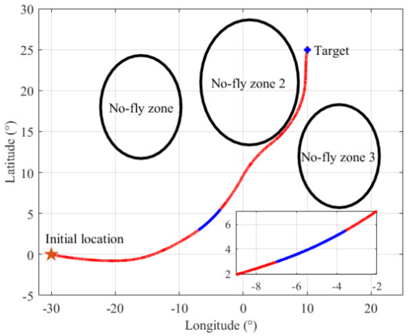
There are three no fly zones, whose locations are given in

Table 1. Locations of no fly zones.

No Fly Zone	Central Position		Radius (km)
	Longitude (°)	Latitude (°)
1	–16	18	700
2	1	21	850
3	15	12	700

. The initial location of the vehicle is set as λ₀ = –30°, ϕ₀ = 0°, and the initial velocity is taken as v₀ = 6500 m/s. The initial altitude is h₀ = 50 km. The vehicle’s initial heading angle and the flight path angle are set as σ₀ = –92°, θ₀ = 0.5°. The location of the target is set as λ₀ = 10°, ϕ₀ = 25°, and the predictor–corrector guidance method developed in [37] is employed to complete flight mission.

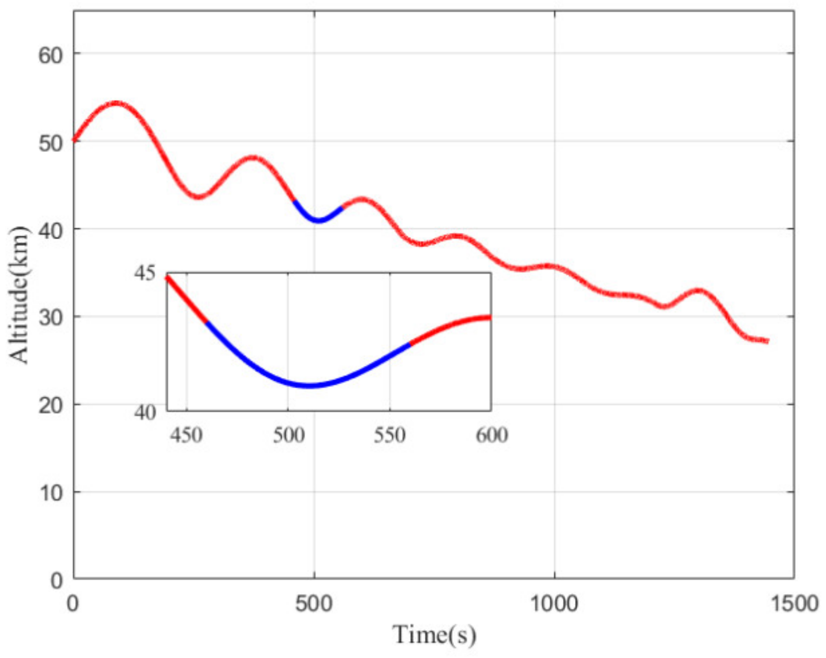
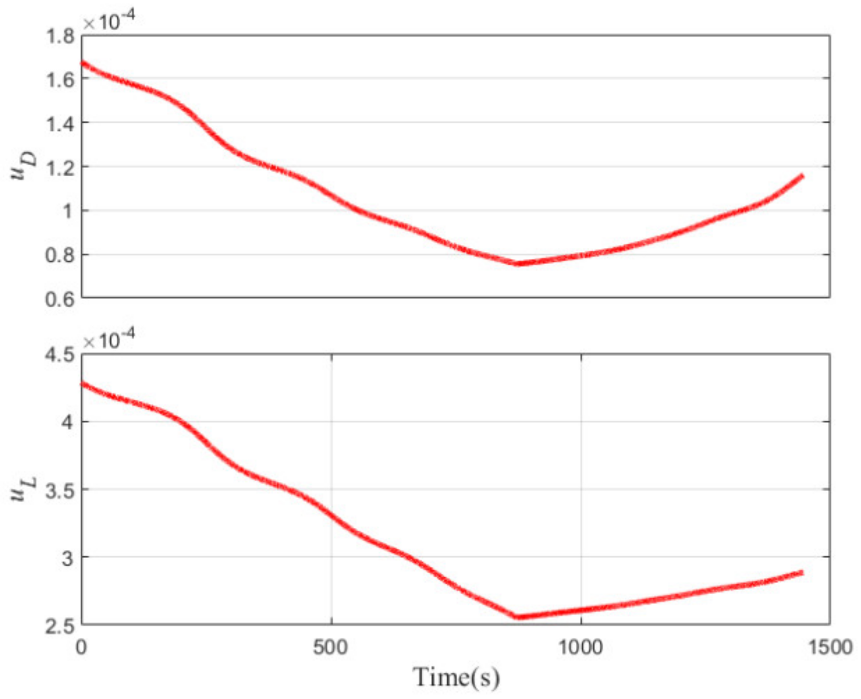
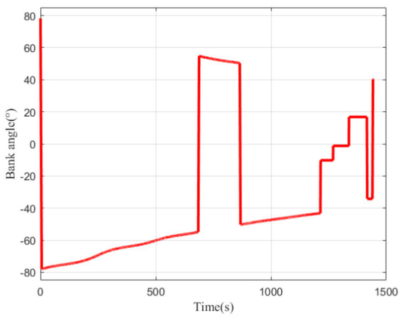
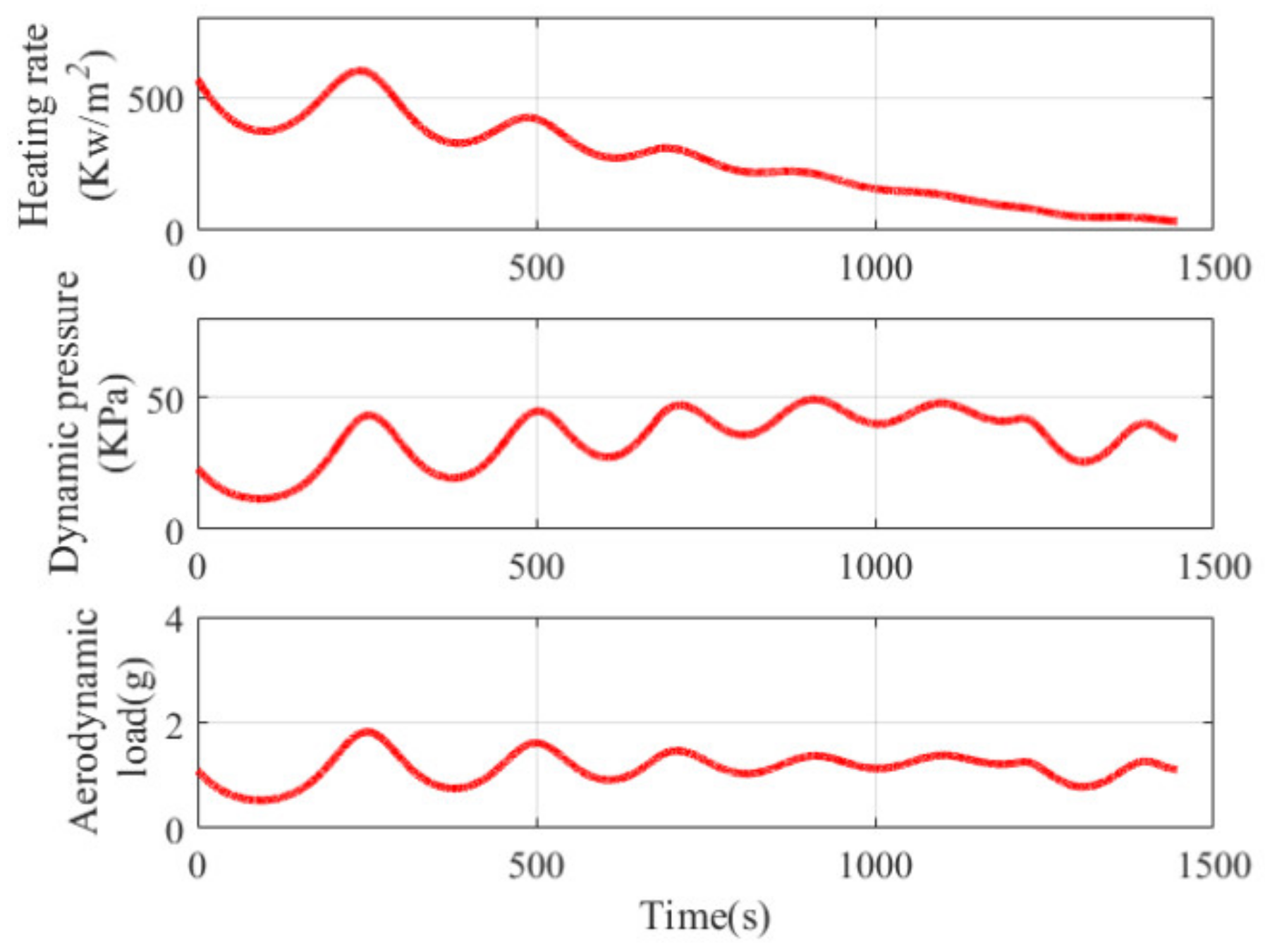
The vehicle’s ground track and longitudinal trajectory are shown in Figure 3 and Figure 4, separately. Figure 5 and Figure 6 depict the quasi-ballistic coefficients versus time and the bank angle versus time in flight, respectively. The inequality path constraints profiles of the vehicle are shown in Figure 7.

As shown in Figure 3 and Figure 4, the vehicle maneuvered both laterally and longitudinally. The vehicle performed a wide range of lateral maneuvers to achieve maneuvering penetration and to avoid the no fly zones with a maneuvering range of thousands of kilometers. Due to the unbalanced longitudinal force, the flight altitude shows the oscillating drop characteristics, which also causes periodic oscillations of the pseudo-ballistic coefficients u_L, u_D, and path constraints shown in Figure 5 and Figure 7. From Figure 5, it can be seen that the quasi-ballistic coefficients u_L and u_D first decrease and then gradually increase after 870 s. This is because the aerodynamic coefficient gradually decreases as the Mach number decreases during the flight, whereas the atmospheric density gradually increases as the altitude decreases, resulting in a gradual increase in the aerodynamic coefficient. It can also be seen that the pseudo-ballistic coefficients u_L and u_D change slowly and within a narrow range. Similarly, path constraints reveal periodic oscillation characteristics within a certain range. As a result, inequality constraints on quasi-ballistic coefficients and path constraints can be imposed in joint state and parameter estimation.

Tracking begins when the target enters the blue area, and the tracking time is set at 100 s. The detection system consists of two sets of infrared detectors on the floating platform. The sampling period is 0.1 s, the standard deviation of angle measurement error is 150 μrad. The position error of the floating platforms is 3 m, and the height and baseline length of the floating platforms are 20 and 300 km, respectively. The following prior inequality constraints are set according to the ranges of the quasi-ballistic coefficients and path constraints in Figure 5 and Figure 7, as well as the fact that the vehicle is continuously turning left:

$$\begin{array}{c}0<\dot{Q}\le {700 \mathrm{kW}/\mathrm{m}}^2\\ 0<q\le 60 \mathrm{kPa}\\ 0.5 \mathrm{g}<n\le 4 \mathrm{g}\\ 0.5\times {10}^{-4}\le u_D\le 1.5\times {10}^{-4}\\ 2.5\times {10}^{-4}\le u_L\le 4\times {10}^{-4}\\ -{70}^{\circ }\le \gamma \le 0\end{array}$$

(55)

Fifty Monte Carlo simulations are carried out to accurately analyze and evaluate the tracking effect of each algorithm. State and parameter estimation results are shown in Figure 8, Figure 9, Figure 10, Figure 11 and Figure 12 and

Table 2. Joint state and parameter estimation results.

Algorithm		Geometric Positioning	EKF	CKF	EKF-MHE	CKF-MHE	Carl-EKF-MHE	Carl-CKF-MHE
Position Error (m)	X	110.8427	37.1287	35.5224	29.9339	28.0366	29.9192	28.5706
	Y	82.4877	27.0623	26.2442	22.6088	21.0697	21.8746	19.8693
	Z	119.3177	35.4530	34.4829	29.9074	28.2527	29.6577	27.8555
	Total	184.3941	58.5029	56.4538	48.3855	45.4477	47.9055	45.0449
Velocity Error (m/s)	X	1108.427	20.9352	18.4407	9.4462	8.3630	8.7439	7.9641
	Y	824.7765	22.0957	21.5234	16.5552	16.1519	16.9394	16.1097
	Z	1193.177	17.9094	15.5532	8.9965	8.2136	8.4998	7.5550
	Total	2607.524	44.2712	39.7885	24.9536	23.4272	28.7505	22.6429
Parameter error	uD (10–5)	−	3.3311	2.4196	2.5320	2.0161	2.2380	1.9410
	uL (10–5)	−	7.1770	6.5862	5.3030	5.0858	5.1732	4.8034
	γ(°)	−	4.5833	2.9116	3.5050	2.5398	2.9110	2.1769
Time cost (s)		−	2.7181	3.4652	32.2073	27.4869	21.1299	18.5042

.

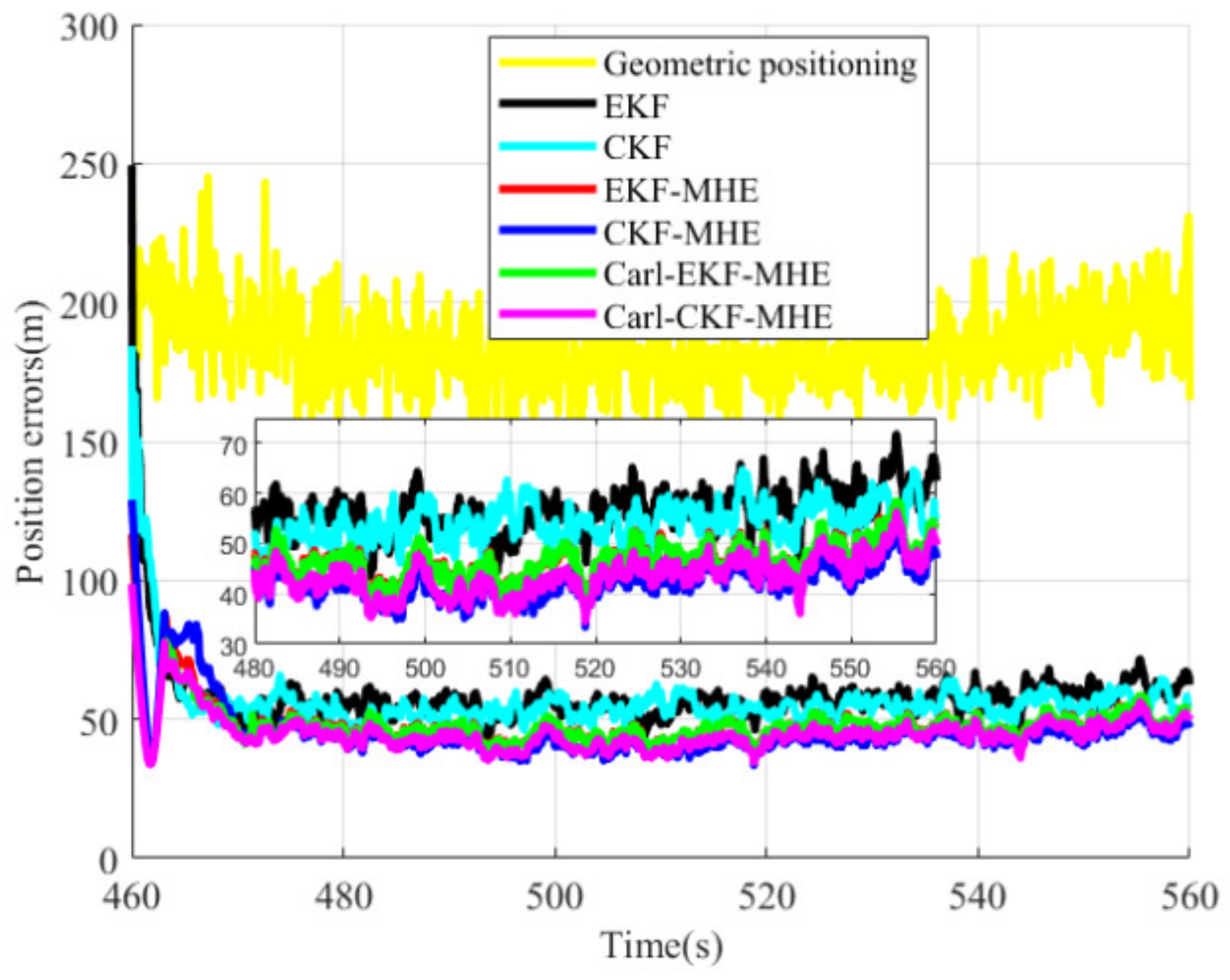
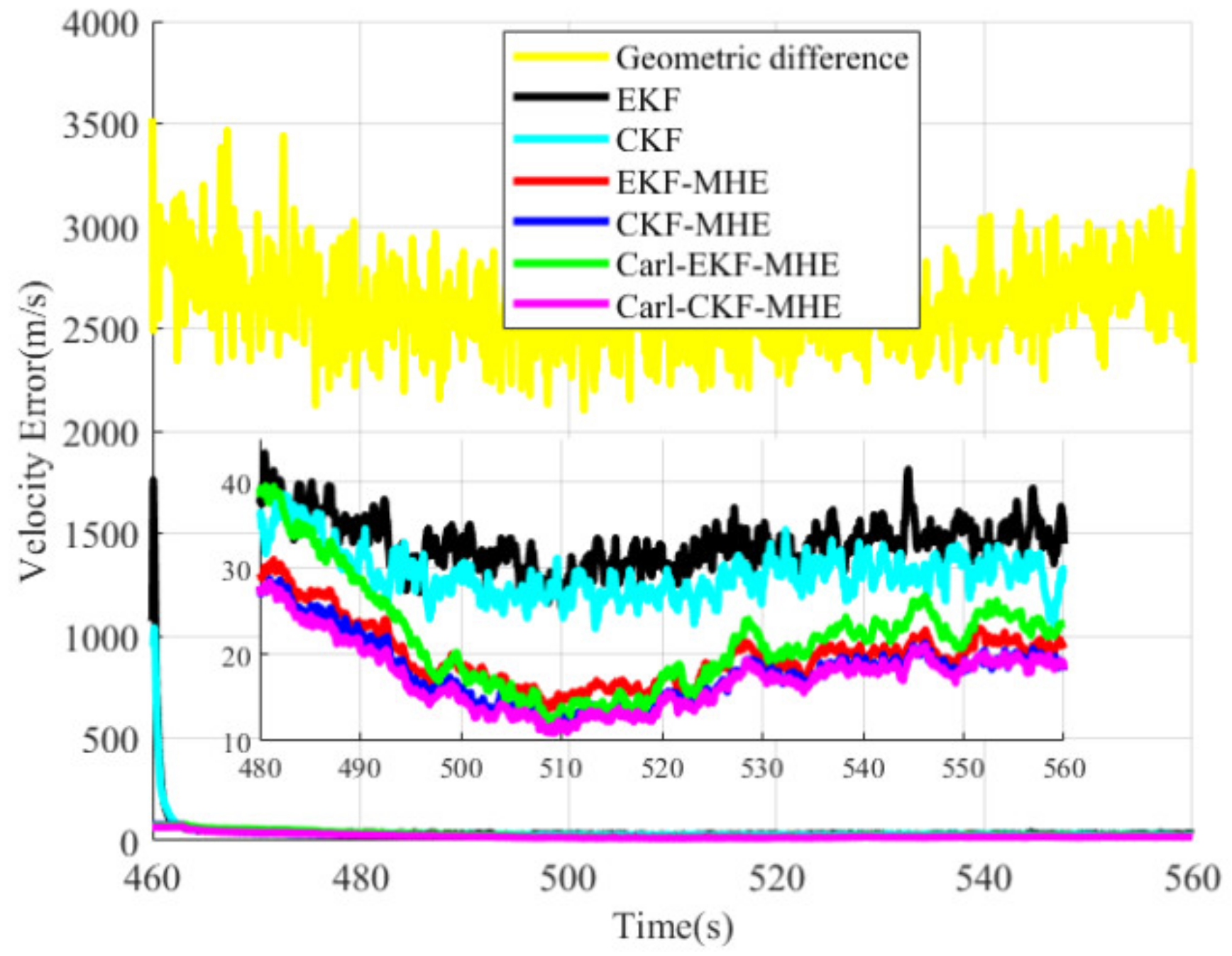
From Figure 8 and Figure 9 and Table 2, it can be indicated that compared with the EKF and CKF algorithms, moving horizon estimation algorithms greatly improve the estimation accuracy and convergence speed of target position and speed. As shown in Figure 8, after the algorithms converge, the position estimation errors of Carl-EKF-MHE and Carl-CKF-MHE are close to those of EKF-MHE and CKF-MHE, respectively, demonstrating the consistency between the linearized model and the original dynamic model. However, in the initial stage, the position estimation errors of the four moving horizon estimation algorithms diverge to a certain extent, which is due to the large initial position estimation error. Due to the strong nonlinearity of the systems in the EKF-MHE and CKF-MHE algorithms, the divergences of these two algorithms are more obvious in the initial stage. It can be seen from Figure 9 and Table 2 that the speed estimation accuracy of Carl-EKF-MHE is lower than that of the EKF-MHE algorithm, whereas the speed estimation accuracy of Carl-CKF-MHE is not lower than that of CKF-MHE. This is because the initial velocity estimation error is large when the EKF is used to update the arrival cost, and there is a large deviation between the linearized model and the original dynamic model. The position and velocity estimation results have indicated that when the initial value and arrival cost are estimated accurately, the linearized model has high consistency with the original dynamic model, and the linearization of the nonlinear system does not reduce the estimation accuracy.

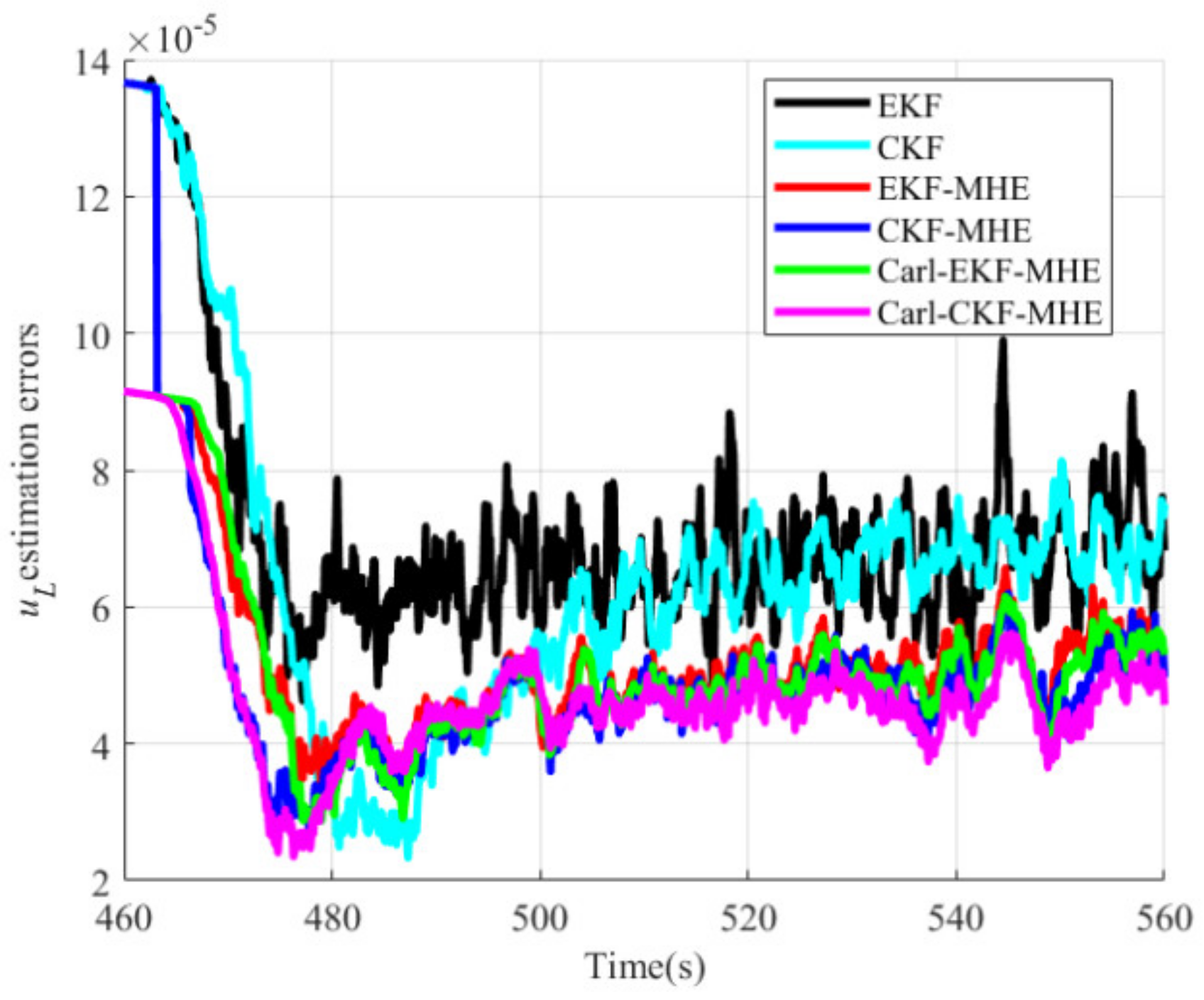
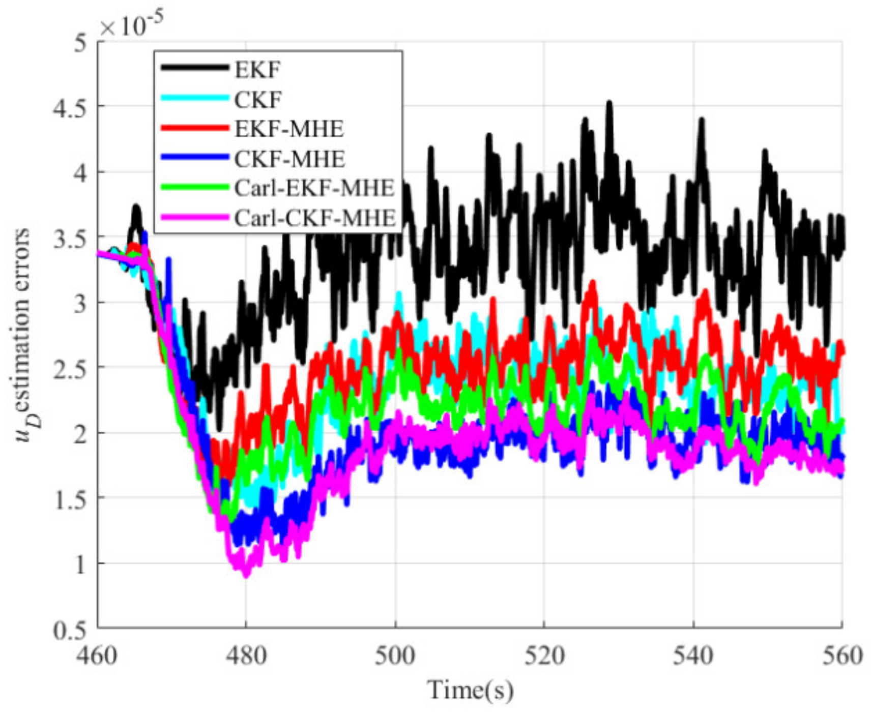
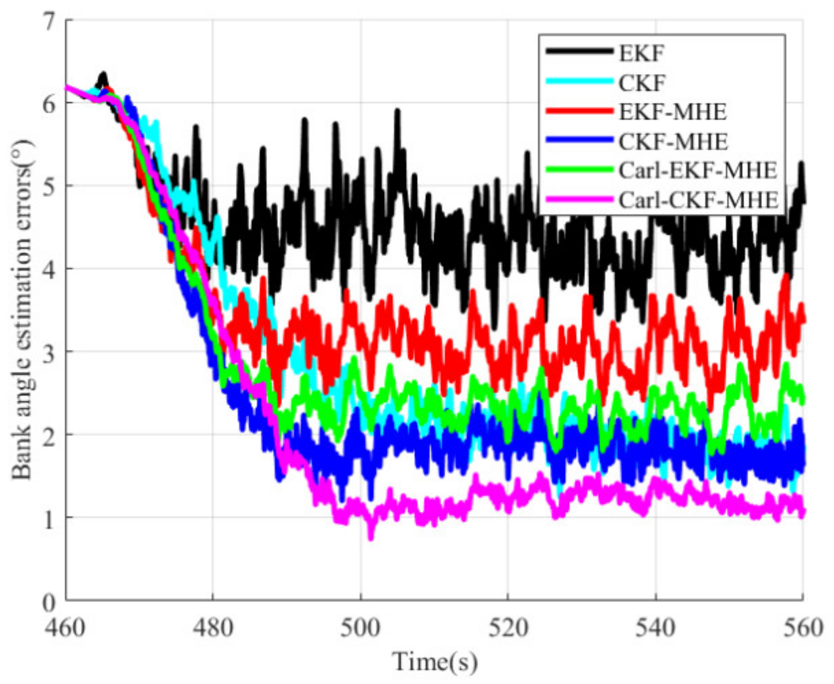
As shown in Figure 10, Figure 11 and Figure 12 and Table 2, the parameters estimation accuracy of moving horizon estimation algorithms is much higher than that of the EKF algorithm. The parameters estimation accuracy of the CKF-MHE and the Carl-CKF-MHE is also much higher than that of the CKF algorithm. This is because, unlike the traditional model-based recursive filter algorithm, in moving horizon estimation algorithms, the parameters are independent optimization variables, and the prior inequality constraints of the parameters are considered. The parameter estimation accuracy of the Carl-EKF-MHE and the Carl-CKF-MHE is higher than that of the EKF-MHE and CKF-MHE, respectively. The reason is that it is easier to converge to the optimal value when solving the bilinear system optimization problem. Furthermore, when CKF is used for arrival cost update, the parameter estimation accuracy is higher than when EKF is used for arrival cost update. This is because using the CKF to update the arrival cost improves the initial state and arrival cost estimation accuracy, as well as the consistency between the linearized model and the original nonlinear system. Moreover, from Table 2, it can be seen that Carl-EKF-MHE and Carl-CKF-MHE algorithms reduce the tracking calculation time by 34.39% and 32.68%, respectively, when compared to EKF-MHE and CKF-MHE algorithms, demonstrating the effectiveness of Carleman linearization in reducing time cost. Carl-CKF-MHE not only has much higher estimation accuracy than Carl-EKF-MHE but also takes less time. This is because a more accurate initial state estimation can significantly reduce the optimization problem’s solution time.

Furthermore, from Table 2, it also can be seen that Cal-CKF-MHE is slightly better than CKF-MHE, the detailed reason is that CKF-MHE realizes joint state and parameter estimation by solving nonlinear constrained optimization problems, while in Cal-CKF-MHE, the nonlinear constrained optimization problems are transformed into bilinear constrained optimization problems by linearizing the nonlinear system via Carleman linearization. Compared with the nonlinear constrained optimization problem, the bilinear optimization problem is easier to solve and has a lower time cost. Meanwhile, the linearized model has been continuously updated as the window slides forward to ensure that it is consistent with the original nonlinear system and it is easier to converge to the optimal value for the bilinear system. Thus, the estimation accuracy of Cal-CKF-MHE is slightly higher than that of CKF-MHE.

The simulation results have indicated that the proposed Carl-CKF-MHE can not only greatly improve the state and parameter estimation accuracy, but can also significantly reduce time cost. The proposed Carl-CKF-MHE can effectively solve the joint state and parameter estimation problems in hypersonic glide vehicle defense. Although the time cost of the proposed Carl-CKF-MHE is lower than that of other MHE algorithms, it is still higher than that of the traditional Kalman filter algorithms, which limits this application to a certain extent. Meanwhile, the proposed Cal-CKF-MHE algorithm needs more prior information about the target than the traditional Kalman filter algorithms.

6. Conclusions

The present work aims at developing a novel moving horizon estimation algorithm via Carleman linearization to solve the joint state and parameter estimation problem in hypersonic glide vehicle defense. By extending the maneuver characteristic parameters that can reflect the target maneuver law into the state vector, the dynamic tracking model applicable to various hypersonic vehicles has been created. To improve the estimation accuracy, the estimation problem has been transformed into a constrained nonlinear optimal estimation problem considering the constraints during flight. For solving the problem of high time cost for solving the nonlinear constrained optimal estimation problem, in the framework of moving horizon estimation, the nonlinear constrained optimal estimation problems have been transformed into bilinear constrained optimal estimation problems by linearizing the nonlinear system via Carleman linearization. The linearized model has been continuously updated as the window slides forward to ensure that it is consistent with the original nonlinear system. To improve the estimation accuracy of the arrival cost, a CKF-based update algorithm has also been introduced to improve the estimation accuracy. The estimation accuracy, applicability, and adaptability of the proposed moving horizon estimation algorithm via Carleman linearization have been tested and validated by simulations. The simulation results have indicated that the linearized model has high consistency with the original dynamic model and that the proposed joint state and parameter estimation algorithm can not only greatly improve the state and parameter estimation accuracy, but can also greatly reduce the time costs. The proposed moving horizon estimation algorithm via Carleman linearization is a feasible and effective method to deal with the joint state and parameter estimation problem in hypersonic glide vehicle defense.