1. Introduction
Electric propulsion is leading to a new focus in aircraft design due to the impact of green technologies on climate change. Moreover, drone flights through thinner atmospheres than earth’s one are raising new challenges on what propeller propulsion can achieve [
1]. These trends require the development of multi-disciplinary optimal propeller design.
The main purpose of this work is to present and test a methodology to design an aero-structural optimal propeller to reduce the energy consumption given a target thrust, airspeed, and environmental conditions. Although the article employs the electric motor equations, a combustion propulsion model can be easily implemented instead [
2].
Intending to optimize the electric aircraft performance, high-reliability models for propulsive systems are required. In the present work, a Blade Element-Momentum Theory (BEMT) algorithm with improved convergence and recursive routines is employed for the propeller performance estimation. Additionally, some corrections to the basic model are implemented to capture the effects of the compressibility, Reynolds number, viscosity, and rotational effects. The rotational correction coefficients are obtained from an adjustment against experimental data [
3].
Despite these corrections, the BEMT accuracy depends significantly on the airfoil lift and drag predictions for each blade’s cross-section. Consequently, some studies employ Computational Fluid Dynamics (CFD) simulations to obtain the aerodynamic data to feed the BEMT method [
4,
5] instead of using Potential Flow Theory (via panel methods) such as XFOIL. Nevertheless, the wide range of studies employing XFOIL requires consideration to conclude which approach is more suitable in propeller design and how significant the difference can be. Therefore, the present work also compares the optimal CFD and XFOIL propeller for the same target conditions.
For the optimization method, a Particle Swarm Optimization (PSO) routine is developed, which guarantees the fulfilment of the target performance and the constraints, including the allowable stress where a structural model based on the Euler-Bernoulli beam theory is used to evaluate the structural viability of the candidate propellers. The PSO methodology has been employed for propeller optimization in different researches [
6,
7,
8,
9], and it also has been reported to be faster than other algorithms such as Generic Algorithms or sine-cosine optimizers [
10,
11].
A case study is carried out to compare XFOIL and CFD optimal propeller results, and the accuracy of the results is discussed through wind tunnel tests. The von Mises stress distribution of the Euler–Bernoulli beam method and Finite Element Analysis (FEA) is also compared while the impact of considering the centrifugal force is evaluated. Finally, the optimal chord and pitch distribution by PSO-BEMT constrained by structural stress are compared to the optimal distributions by Euler–Lagrange equations applied at vortex theory (Goldstein distributions) [
12,
13]. Finally, the results of the CFD propeller are compared to experimental data of a commercial propeller with the same diameter, pitch, and operational conditions.
Recent studies have assessed only optimal build materials for propellers through CFD-FEA analysis coupled with optimization techniques to minimize the failure index, which resulted in an optimum laminate with unbalanced nonsystematic stacking [
14]. Additional studies have carried out propeller optimization through space mapping surrogate modeling coupled with open source propeller analyses and design programs such as QPROP, and the latter has resulted in an optimized design where the propeller geometry is suggested [
15].
This research seeks to expand and contribute in different ways, such as the presentation of a BEMT algorithm with improved convergence and recursive routines that have not been exposed before for propellers [
16], the implementation of a constrained PSO routine for a multi-disciplinary propeller optimization, the investigation of the airfoil geometry distribution along an optimal blade considering structural restrictions, proposal of the specific coefficient values of the rotational correction for small propellers (values in literature are for much larger rotors and for wind turbines that operate at considerably lower rotational speed [
17,
18,
19]), testing of the feasibility of printed propellers, proposal of an equation to correct the stalling angle for different Reynolds numbers, validation through FEA the Euler–Bernoulli beam theory applied for propellers, and conclusion about the suitability for a BEMT fed by XFOIL and CFD. Moreover, some previous works do not manufacture the optimal solutions to validate the results or do not consider the interaction of the propeller efficiency with the motor efficiency [
2,
9].
2. Airfoil Aerodynamic Data
One of the main inputs that composed the global model is the aerodynamic data associated with each airfoil located over the propeller span-wise section. Therefore, a parameterization method with a few parameters that are available to describe a wide range of geometries is required and that is the main reason why the 4-digit NACA method is selected for this study [
10]. The 4-digit NACA airfoil shape is defined by the thickness
t in chord hundredths, the maximum camber
z in chord hundredths, and the maximum camber position
in chord tenths. The airfoil shape equations in terms of these parameters can be found in the literature [
20].
Aerodynamic data for each airfoil requested during the optimization process is computed through the potential flow-based software XFOIL or with the finite volume open source software OpenFOAM. To keep a low computational cost, and due to the limitations of XFOIL and Reynolds-averaged Navier–Stokes (RANS) models accuracy for highly separated flows [
21], a Montgomerie extrapolation method [
22] for both lift and drag coefficients is employed beyond the stall angle.
2.1. XFOIL
XFOIL is a computational implementation of the panel method coupled to an integral boundary layer formulation and a
laminar to turbulent transition technique [
23]. This tool allows predicting
and
at small angles of attack, preferably before stall. A routine is developed to connect with XFOIL and extract
and
data for any local blade section, operational condition, and airfoil shape. In case of divergence, a recursion within the code is applied, increasing the nodes over the top and bottom surface of the airfoil and the maximum available iterations during the calculation. The initial setup is defined with 150 maximum iterations and 200 nodes over the airfoil surface, and a smoothing step fixing avoiding any high variation of the coordinates is also applied.
Aiming to decrease computational cost for other optimization cases (where similar data might be needed), a database is created with the purpose of saving every airfoil datum that it is analyzed.
2.2. CFD
OpenFOAM is an open-source software that solves the main governing fluid equation over the discretized computational domain through the finite volume method, which also allows implementing different turbulence models [
24]. Furthermore, a routine is developed to define any desired simulation setup based on each local blade section and operational condition to compute required data automatically during the optimization process.
2.2.1. Grid Independence
A grid independence analysis is performed to obtain the minimum number of cells, which provides steady results at a reasonable computational cost, the study is carried out with a NACA 0015 airfoil at a Reynolds number of
and
°, volumetrics elements were increased from
up to
cells. According to the results, a steady behavior and convergence was obtained at
number of cells approximately. The results are shown in
Figure 1.
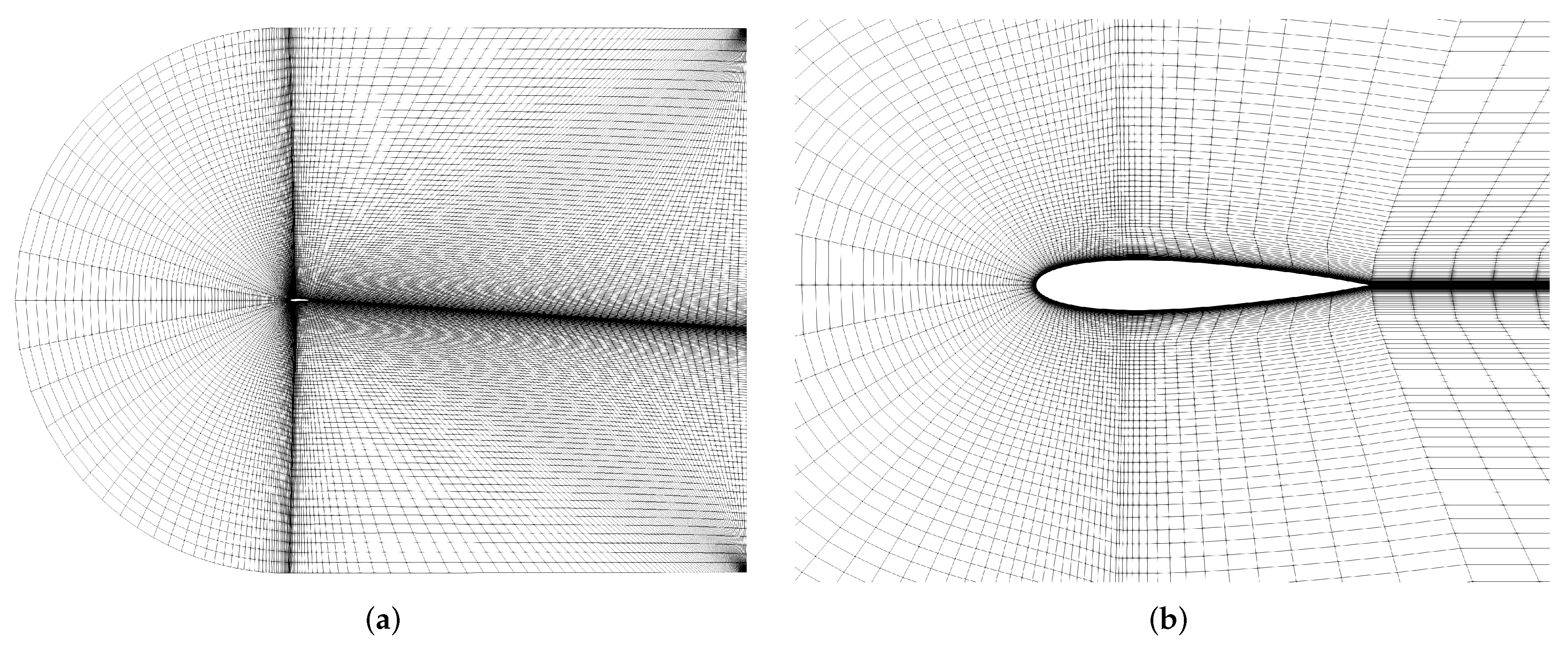
2.2.2. Mesh Topology
The mesh is generated automatically with an elliptical or hyperbolic algorithm to generate a structured C-Grid topology. The mesh parameters are tuned to fulfill the mesh quality standards and independence.
The mesh is set with
number of cells, providing accurate data with low computational cost. In terms of mesh quality, a
is guaranteed [
25] employing the flat-plate boundary layer theory ([
26], p. 467), where
is the non-dimensional wall distance. Finally, the average cell skewness angle is close to 0, and the average cell aspect ratio is under 30. The mesh is shown in
Figure 2.
2.2.3. Simulation Setup
The simulation is performed with a steady-state time scheme and Gauss linear divergence scheme [
27], and the convergence criteria are set as
for the residual of the fluid variables and relaxation factor of
for all fluid variables. The SIMPLE algorithm is defined for the calculation process. The upstream domain, composed of the left, top, and bottom sides, is defined as a velocity inlet boundary condition. The downstream domain side is set as a pressure outlet boundary condition with gauge pressure equal to zero, and the airfoil surface is defined as wall boundary with the no-slip condition. The angle of attack is guaranteed by setting the respective wind speed
and
components to use one single mesh for any angle. The routine computes the normal and axial aerodynamic forces over the airfoil. Hence, they must be transformed into the relative wind reference frame and normalized to obtain the lift and drag coefficient. A four-equation Langtry–Menter
SST turbulent model is employed, which adds two other equations: one for the intermittency
and other for the laminar-turbulent transition with
criteria, which links empirical transition data with the intermittency equation [
28].
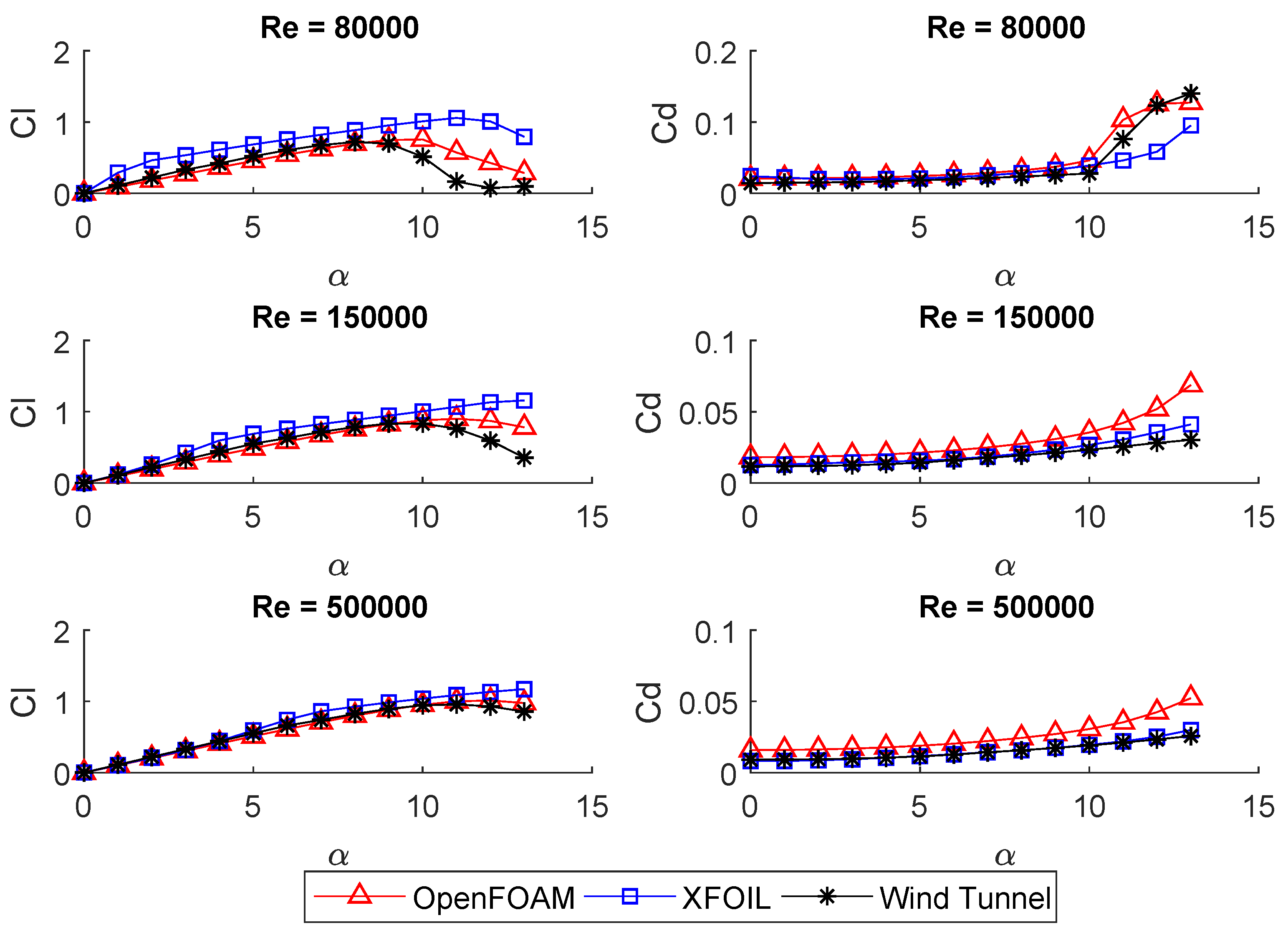
2.3. Validation
Aerodynamic coefficients are computed for the NACA 0015 airfoil through XFOIL and CFD (OpenFOAM) and are compared against experimental data reported by Selig et al. [
29], from
° to
° at a Re numbers of
,
,
. The results are shown in
Figure 3.
From the results obtained, the lift coefficients extracted from CFD OpenFOAM and XFOIL present an average error of 5.21% and 8.23%, respectively, highlighting the stall prediction by the finite volume software, which is a relevant indicator during airfoil performance calculations. The OpenFOAM prediction at a low Reynolds number where the flow separation phenomenon occurs is also remarkable. The average error associated with is 8.09% and 6.78% for CFD OpenFOAM and XFOIL, respectively.
3. Electric Propulsion Model
The main three parameters in propeller metrics ([
30], pp. 566–568) are the advance ratio
J (Equation (
1)) used to quantify the effects on forward motion and rotational speed, the thrust coefficient,
and torque coefficient,
(Equation (
2)). Usually, propellers operate at
J values from 0 (static thrust) to 1.4 [
3].
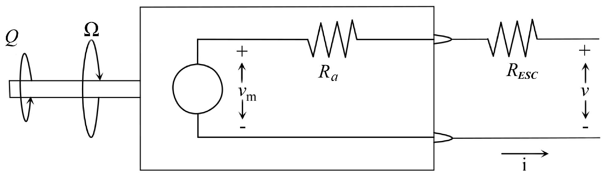
The behavior of a Direct Current (DC) electric motor is described by the equivalent circuit shown in
Figure 4 and the equations from Equations (
3)–(
5).
For an electrical propulsion system, three efficiencies affect its performance: the electrical efficiency (Equation (
6)), the propeller efficiency (Equation (
7)), and the controller efficiency. As the last of the efficiencies approaches one at high PWM frequencies or high power [
32], it is decided to neglect it from this work. Therefore, the two first efficiencies result in the total efficiency (Equation (
8)) [
33].
4. Structural Model
The main propeller forces are the torque, thrust, centrifugal force in the axial direction, centrifugal twisting, and aerodynamic twisting forces. In the present study, only the first three are considered in the stress estimations. The Euler–Bernoulli beam theory is employed to determine the stress along the blade. This theory has proven to work for ratios of 10 or higher and has been previously used in blades design [
34,
35].
The magnitude of the centrifugal force at a section
is estimated through Equation (
9).
The magnitude of the bending moments due to the axial and tangential forces in the blade at radius
are computed and then projected onto centroidal axes through Equations (
10) and (
11). The main centroidal axis is assumed to be parallel to the chord line.
Finally the normal stress at certain cross-section points is calculated employing Equation (
12).
According to the sign convention employed,
x is positive from the centroid towards the trailing edge and
y from the centroid towards the extrados. To estimate the shear stress, the airfoil is approached as a rectangle of an equivalent area [
31,
36]. The maximum shear stress due to torsion on a rectangular shape is given by Equation (
13) [
37].
where
t is the thickness and
c is the length of the equivalent rectangle, and the torsional moment
applied to the cross-section at radius
is estimated through Equation (
14).
where
are the centroid coordinates and
are the coordinates of quarter-chord, where the aerodynamic forces are assumpted. For the cases when the blade is made of some isotropic material, the von Mises criteria for allowable stress can be employed as is shown in Equation (
15), where the maximum shear stress is used to obtain a conservative estimate.
Finally, the structural constraint is defined as , where is the safety factor, and is the yield tensile strength.
5. BEMT Model
5.1. Overview
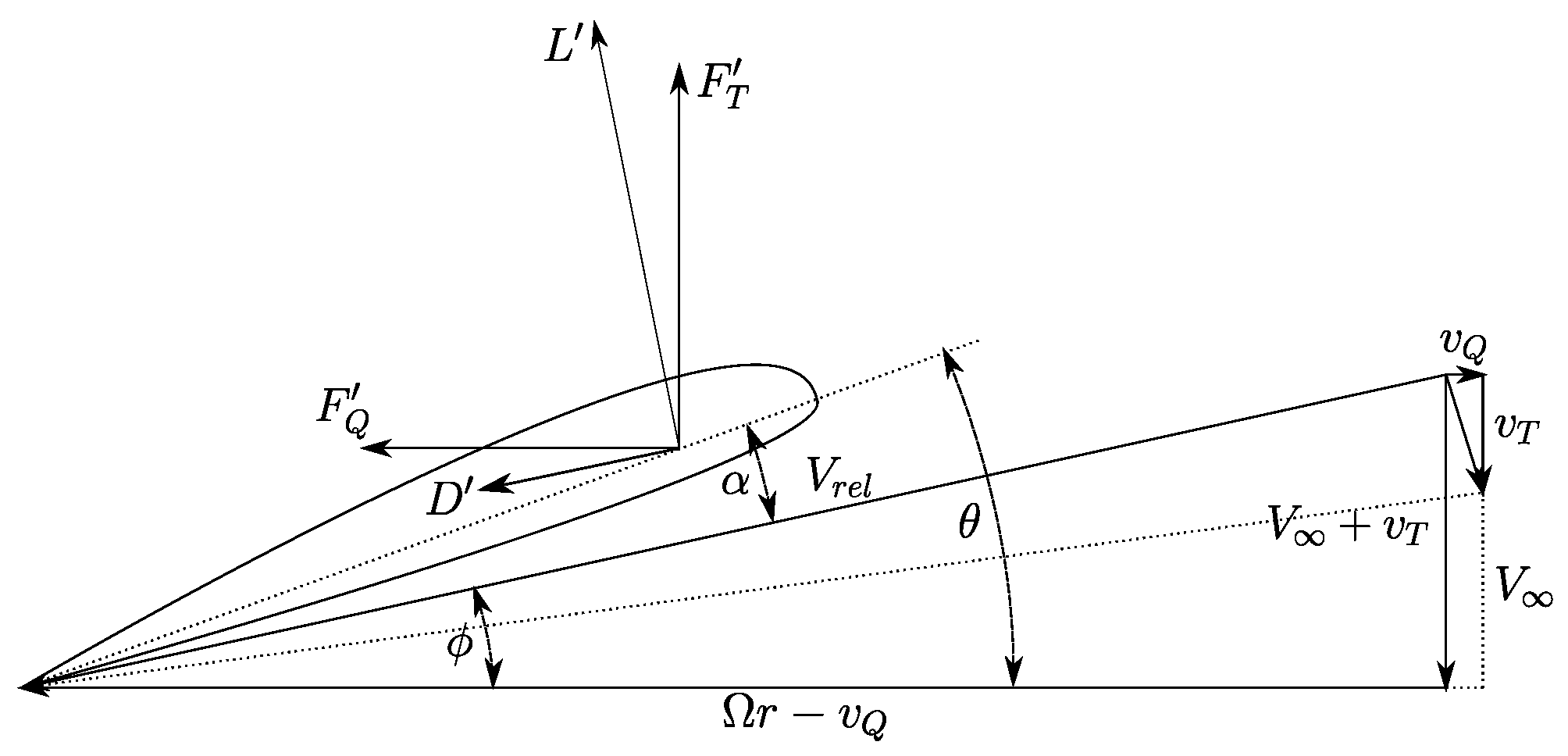
The BEMT method is a relatively simple tool for rotor performance analysis. For a given operational condition and a known propeller geometry, thrust, torque, propulsive efficiency, and force distributions can be estimated by combining the Blade Element Theory and One-dimensional Momentum Theory. The Blade Element Theory deals with relative velocities and angles, while the Momentum Theory deals with the relationship between velocities at different flow points. Glauert presents a detailed description of both methods in [
38]. This method divides the blade into a certain number of discrete and independent blade elements for which, through an iterative process, local induced velocities can be estimated and hence, resultant forces along the whole blade. The method has to be fed with a reliable database of aerodynamic coefficients for the present airfoils along the blade to estimate lift and drag forces for each blade element at the estimated angle of attack and Reynolds number. Note that according to
Figure 5, the angle of attack depends on the local pitch angle, which is fixed, and the local inflow angle. Then, in order to estimate
, all velocities on the blade must be known: axial, tangential, and induced. Both components of induced velocity (
and
, see
Figure 5) are calculated through an iterative process; then, estimated lift and drag forces are rotated into their axial and tangential components (
and
, see
Figure 5), which were calculated along each blade element and integrated into total thrust and torque, as shown on Equations (
16) and (
17).
5.2. Improved Convergence
Ning [
16] presents a BEMT method for wind turbines with guaranteed convergence. The work assesses some convergence issues at the wind turbine solution. However, only one of those convergence issues can be assessed for aircraft propellers due to its different operational regimes. Then, the BEMT method for propellers does not achieve a hundred percent convergence rate. However, it is considerably improved. The equation for the axial induction factor (Equation (
18)), is only valid when
(See Equation (
19)) is not higher than 1.
The solution is improved by modifying the value of on the iterative process when it exceeds the unity. When this happens, the value for the axial induction factor is unreasonably high, and it only happens in the convergence process, sometimes breaking it. When the BEMT is about to converge, takes much more reasonable values of induction factors. Then, in the convergence process, values of higher than one are modified to 0.99, giving stability to the convergence process. These cases result in an induction factor of 99, a value completely unreasonable that goes down while approaching convergence. Additionally, a relaxation factor to improve the convergence stability is applied with recursion. Finally, the BEMT routine is run again with a lower relaxation factor when convergence is not achieved.
5.3. BEMT Sections Independency
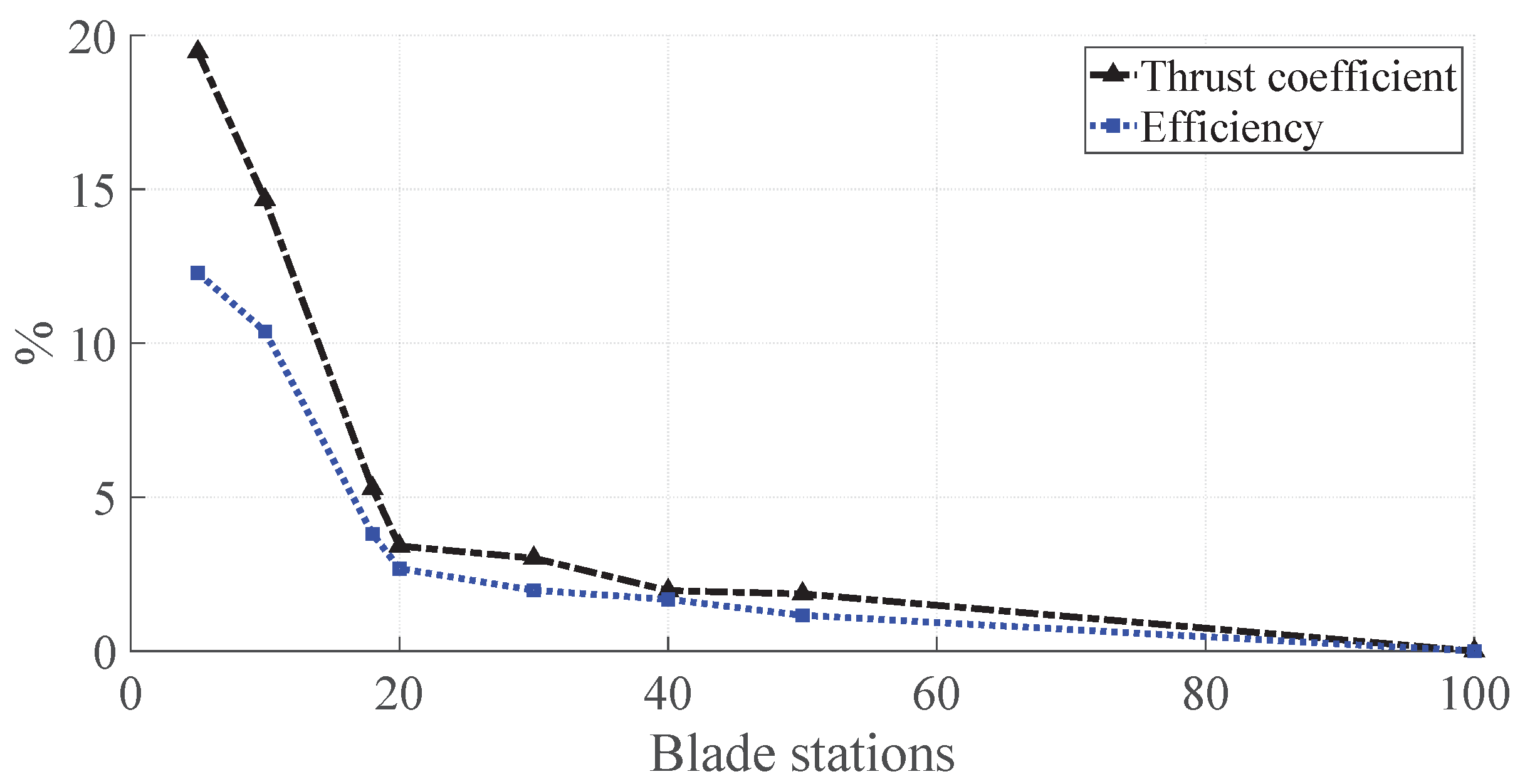
The BEMT method divides the blade into a discrete number of sections. The number of divisions of the blade has to be chosen carefully, so the technique presents accurate enough results while keeping a reasonable computational cost. An analysis is carried out to assess the most suitable number of stations for small-sized propellers, which is the design space of the case of study due to the wind tunnel limitations. Hence, a set of simulations using 5 to 100 divisions are run and the difference in results is compared to the finest distribution of stations (100).
Figure 6 shows the percentage relative difference between the results obtained with a different number of stations and the results obtained with 100 stations. According to the results, 20 is selected as a suitable number of stations with a difference of 2.7% for efficiency and 3.4% for the thrust coefficient in comparison to the 100 stations results.
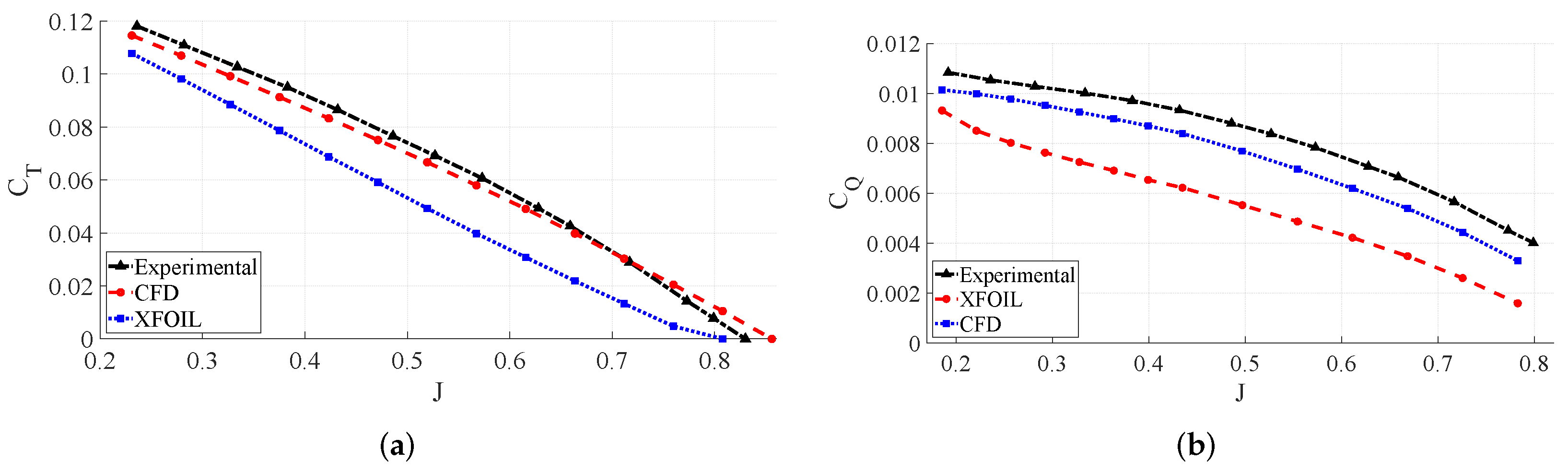
5.4. BEMT Model Validation
The method has to be validated to ensure that predictions carried out in the optimization routine are reliable. Performance predictions are computed for the APC 10X7 propeller, and results are compared to experimental data available in the UIUC Propeller Database [
3].
Figure 7 shows predicted and experimental
and
vs.
J curves.
The results show that XFOIL and CFD have their minimum difference at the lowest J value, which is the regime of higher Reynolds [
39]. Moreover, CFD shows a higher fitting with experimental data (especially for thrust), due to the difficulties obtaining an accurate drag prediction which is more related to the torque coefficient.
5.5. Corrections
The aerodynamic coefficients require some corrections to approach the variety of phenomena not included in the XFOIL or CFD data acquisition. Compressibility account for the changes in the lift and drag coefficients mainly for a Mach number (
M) higher than 0.3. To capture this phenomenon, the Karman–Tsien correction [
40,
41] for both coefficients is employed. A method to estimate the tip losses by Prandtl is also applied. Finally, to consider the effect of centrifugal force and the Coriolis effect, the approach presented by Chaviaropoulos and Hansen [
17] is implemented.
5.5.1. Rotational Correction Adjustment
The semi-empirical method is developed for wind turbines but it can also be used for propellers. The model employs three empirical parameters that can be problem-dependent
a,
h and
b (see Equations (
20) and (
21)). The original notation for these coefficients is modified in this work to avoid confusion.
where
is the difference between uncorrected lift coefficient and the inviscid lift coefficient; similarly,
is the difference between uncorrected drag coefficient and the minimum drag coefficient.
According to [
17],
,
, and
, which are values that had been used in other studies ([
18,
19]). Nevertheless, these parameters come from a wind turbine blade with a NACA 63-215 airfoil, which rotates at a considerably lower speed than propellers. Therefore, these coefficients correspond to less significant centrifugal and Coriolis effects and an NACA 63 airfoil family.
An optimization study to reduce the error between the BEMT predictions in comparison with a set of experimental data of APC propellers with diameters from 0.2032 to 0.381 m [
3] is carried out to estimate the parameters that have the best fitting to this kind of rotor, from which the results are the values
,
, and
.
5.5.2. Prandtl’s Tip Approach
Prandtl developed a factor to correct the load distribution along blade radius to account for the losses for having a finite number of blades. The approach is shown in Equation (
22) [
42].
5.5.3. Mach Correction
At high rotational speeds, the compressibility effects can become significant, especially towards the blade tip. However, the implemented XFOIL and CFD routines do not consider this phenomenon. Hence, the lift and drag coefficients feeding the BEMT method are corrected by the Karman–Tsien correction [
40,
41]. The drag coefficient correction is shown in Equation (
23), which is also valid for the lift coefficient.
5.5.4. Drag Coefficient Correction
Given the convergence issues at low Reynolds, XFOIL and CFD data are not calculated directly at this condition. When some blade section has Reynolds below 80,000, the drag coefficient at 80,000 is employed and then corrected by Equation (
24) [
43]. This correction is also implemented when the airfoil can not converge in XFOIL or CFD even at Reynolds higher than 80,000, then the value at which it converges is employed for the correction.
5.5.5. Stall Angle Correction
The latter situation also affects the accuracy of lift data. The linear region of the lift curve does not considerably change with Reynolds. On the other hand, the stall value is affected meaningfully, but there are no corrections in the literature. Equation (
25) is a simple way to consider the aforementioned effect, which has a similar expression of the drag correction but with a power value calculated, reducing the error from experimental NACA airfoils data [
44] between Reynolds of 10,000 and 160,000.
6. Optimization
6.1. Optimization Problem
This optimization problem aims to reduce the electric power required from the battery while fulfilling the target thrust at a certain cruise speed. The battery pack is chosen by the voltage required to drive the propeller in the optimization results. The optimization routine estimates the combination of propeller pitch and chord distributions, as well as the airfoil shape along the blade and the rotational speed that minimizes the energy consumption of the aircraft propulsion system; those are the defined optimization variables. Some constraints are applied to guarantee the safety and viability of the operation: the maximum motor power, the maximum propeller diameter, the maximum voltage, and the stress limit defined by the yield point of the material should not be exceeded. Therefore, different extremals can be reached for different propeller materials, where higher strength and rigidity would reduce power consumption.
A way to approach the drag of the aircraft at the design condition taking into account the increase in drag due to propeller wake influence
can be found in [
2].
The bespoke routine of optimization was developed in Matlab on a Linux-based system to allow the integration to OpenFOAM and XFOIL via console commands.
6.2. Particle Swarm Routine
The Particle Swarm Optimization (PSO) method is an evolutionary algorithm that aims to find the optimal point of some fitness function by swarming a set of particles among the search space. The search space has as many dimensions as optimization variables and represents all their possible combinations. Then, for this work’s case, the search space is the set of all possible propeller designs, including rotational speeds. Initially, a set of particles is randomly allocated all over the search space, each location corresponding to a specific combination of optimization variables. Then, the fitness function is evaluated for each of them, and the swarming process begins. The particle that performs best will become a reference to which the other particles will be attracted. All particles among the search space will move some distance towards the reference particle, and then the location of each one will be updated. All new locations are evaluated, aiming to find a new particle that performs even better than the previous reference. This way, all particles will move along the search space, evaluating different combinations of optimization variables aiming to find the position in the search space that satisfies the fitness function better. Eventually, after some time, all the particles are expected to converge to a single point in the search space that is at least a local maximum (for this case, the algorithm aims to maximize). The particle’s movement can be stopped after converging to a single point or after a fixed number of iterations. To promote a broader movement along the search space to look for possible new bests, the particles will be attracted to the reference particle and to its own best position of its history. This allows a broader exploration of the search space aiming to avoid the convergence to possible local minima.
The movement of the particles is dictated by Equations (
26) and (
27). The ⊗ symbol stands for element-wise multiplication.
The first term in Equation (
27) limits the movement of the particle so it does not start moving out of the bounds of the search space, causing the algorithm to be unstable. The second term represents the attraction to the instantaneous global maximum (the reference particle), and the last term represents the attraction to the best position in the history of each individual particle. Parameters
and
allow to give weights to both attractions, and vectors
and
generate some randomness to the movement of the particles to promote the exploration of the search space even more. They are N-dimensional vectors with randomly generated entries between 0 and 1.
As mentioned above, pitch, chord, thickness, distributions of maximum camber and maximum camber location, diameter, and operational rotational speeds are taken as optimization variables. Pitch and chord distributions are defined with four radial points defining a cubic spline for the whole distribution. Thickness, camber, and camber location are determined similarly but with three radial points, then having a total of 19 optimization variables. In order to assure that the optimal propeller at the end of the routine fulfills the aforementioned established restrictions, a penalty function is applied to the particles that do not meet them. This way, they would not attract others to that position in the search space.
and
are set both at 2, giving equal weight to individual and global partial optimal design for the movement of the particles. Those are sensible values when a wider search is desired [
45]. The parameter
has to be set with some trials. For this case
ensures the particles do not move too fast, preventing them from moving too far from the desired search space. This avoids the evaluation of unreasonable propellers.
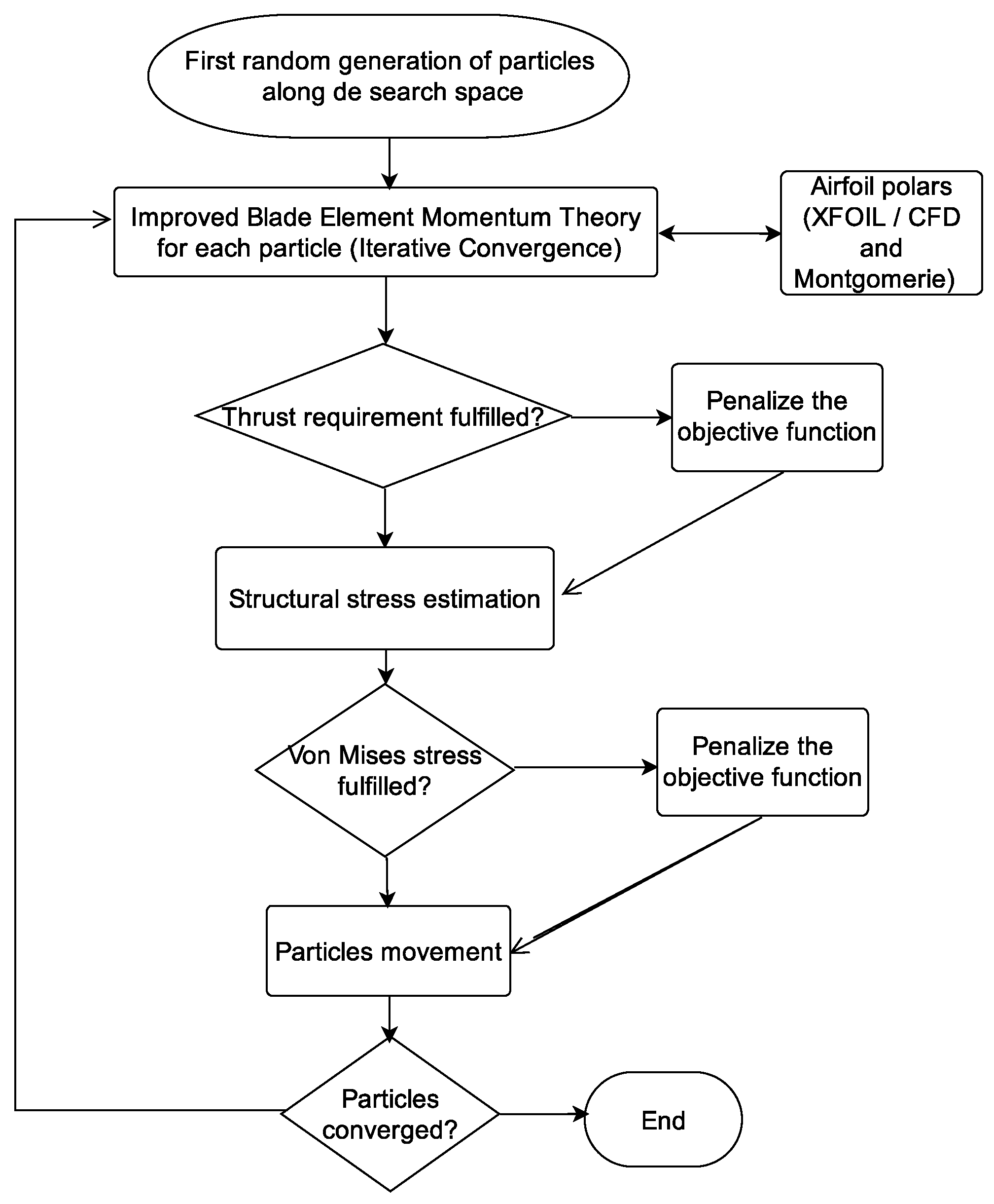
Figure 8 shows the general scheme of the optimization. However, specific details are not explicitly shown, such as the recursion of the XFOIL, the iterative convergence of the BEMT, corrections of 2D airfoil data, or the electric model. Basically, a set of random propellers is generated. They start varying their design parameters as the algorithm evolves, and that variation is restricted by penalizing the designs that do not fulfill structural or thrust requirements. The fitness function of each design is evaluated through BEMT, which at the same time provides enough data to check additional constraints (thrust and structural).
7. Case of Study
The set selected for the optimization is the Hacker A50-10L Turnado controlled by the Phoenix Edge HV 80 ESC. Although the proposed method should work for any propeller size, the diameter is restricted by the available wind tunnel section.
Table 1 shows the design parameters.
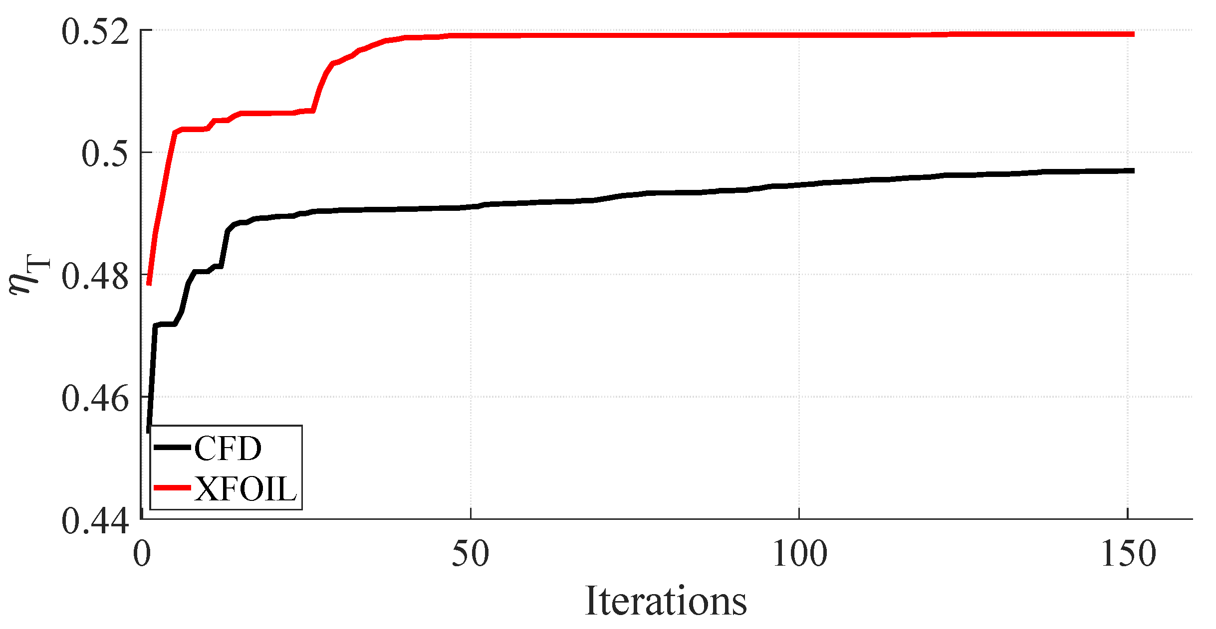
7.1. Results
The PSO iterations are shown in
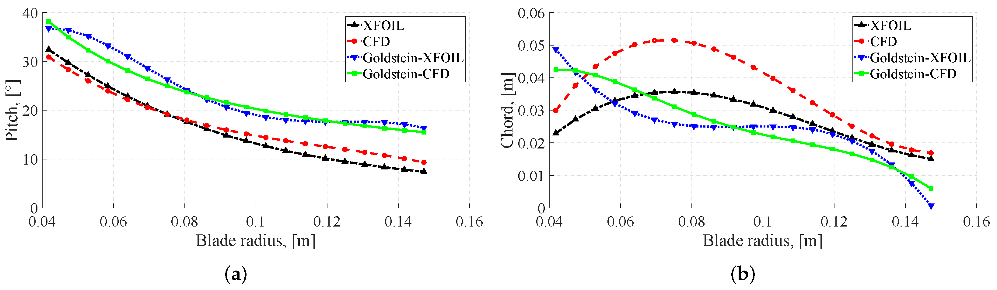
Figure 9 against the total efficiency. The higher the total efficiency, the lesser power consumption of the system, which relates the motor and propeller efficiency. The pitch and chord distributions for the optimal CFD and XFOIL propellers are shown in
Figure 10. Additionally, the distributions are compared against Goldstein distributions, which are the optimal pitch and chord calculated through the Euler–Lagrange equations applied to vortex theory. Some details about how to calculate these distributions can be found in [
9]. Nevertheless, the Goldstein distributions are unique for given trust, airfoil distribution, and operational conditions having a considerably lower computational cost; hence, these distributions are analyzed for looking at an insight, which allows reducing the current computational cost of searching a distribution with a PSO that fulfills the target thrust while minimizing the torque. Moreover, in [
9], the thin propeller results also showed the difficulty of optimizing the propeller aerodynamic without considering the structural constraints. However, similar airfoil thickness and camber distributions (with a minimum value somewhere between tip and root) were obtained in that study (nevertheless, the airfoil design space is different).
The results from
Figure 10 show a similarity in the pitch distribution between XFOIL and CFD. On the other hand, the chord distributions are considerably different, which means that the pitch distribution is less dependent on variations of airfoil selection and aerodynamic coefficients, with the chord more sensitive. Moreover, the CFD chord is larger than XFOIL, which means that XFOIL overpredicts the lift coefficient, requiring less chord than CFD predictions.
Regarding the optimal vortex distributions (Goldstein), the chord trend is different in shape and values, with these vortex propellers being thinner, which probably implies non-compliance with structural constraints. The vortex pitch distribution presents higher angles, also affecting the structural stress; nevertheless, the shape of the curve is meaningfully similar to PSO-BEMT distribution, especially for the CFD airfoils, with a constant offset of about . The latter results suggest that the spline parameterization of pitch and its coefficients can be replaced for the Goldstein distribution plus an offset parameter, which would reduce the computational cost meaningfully, especially when CFD coefficients are employed.
It is expected that a larger propeller operates at a higher Reynolds number. However, for the same thrust, varying the diameter could also change the rotational speed and chord, impacting the Reynolds number. On the other hand, if we compare the structural stress caused at the propeller root to a particular new section of the propeller which generates additional thrust being at the tip (increase diameter) or at the middle (increase chord), the torque and the centrifugal force created by the first one would be higher than the second case. In other words, it is probably more efficient for structural stress to create thrust near the root (increasing chord) than increasing diameter, which is perhaps why the optimal diameter did not reach the maximum, even though it almost does.
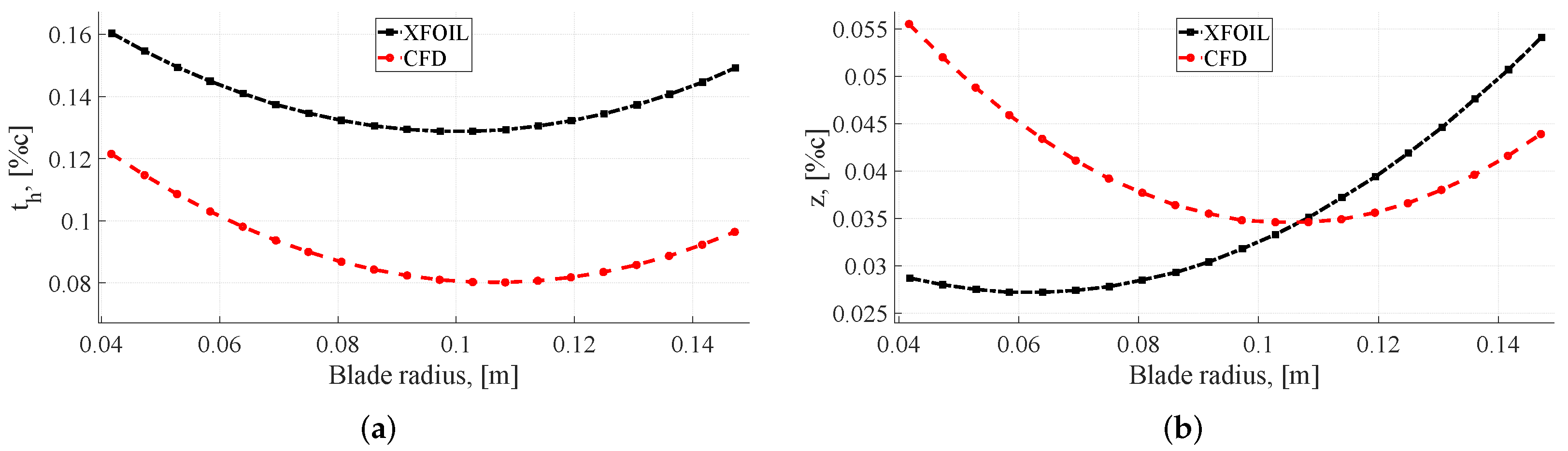
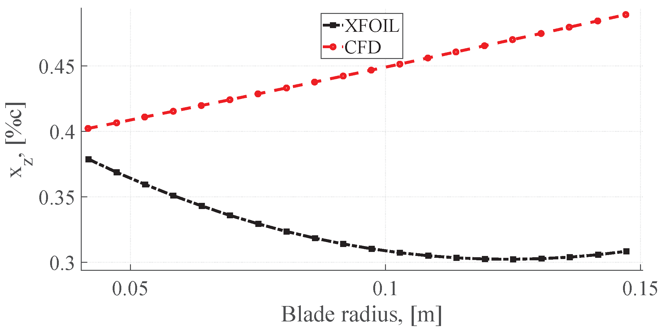
The airfoil distribution can be summarized with the thickness, maximum camber, and maximum camber position (naca 4-digits). These distributions are shown in
Figure 11 and
Figure 12. The trend of the XFOIL maximum camber position shows a highly curved airfoil towards the leading edge which increases the lift but the drag would create a separation of the boundary layer. The limitations of XFOIL in drag and stall prediction are probably why the optimal airfoil distribution has its shape, while CFD has a more smooth extrados surface similar to an arc, preventing boundary layer separation.
Regarding the camber distribution, the XFOIL and CFD show equal values about the middle of the blade, where the Reynolds number is usually maximum [
39]. It is in agreement with the results of 2D airfoil data. The main difference in camber distribution is at the root, where CFD generated a highly cambered airfoil, while XFOIL estimated a more conservative camber. It is probably explained by the low Reynolds difference between the two methods, where CFD captures a more significant impact in airfoil performance, requiring a higher camber to reach the same lift at this section.
7.2. Structural Results and Validation
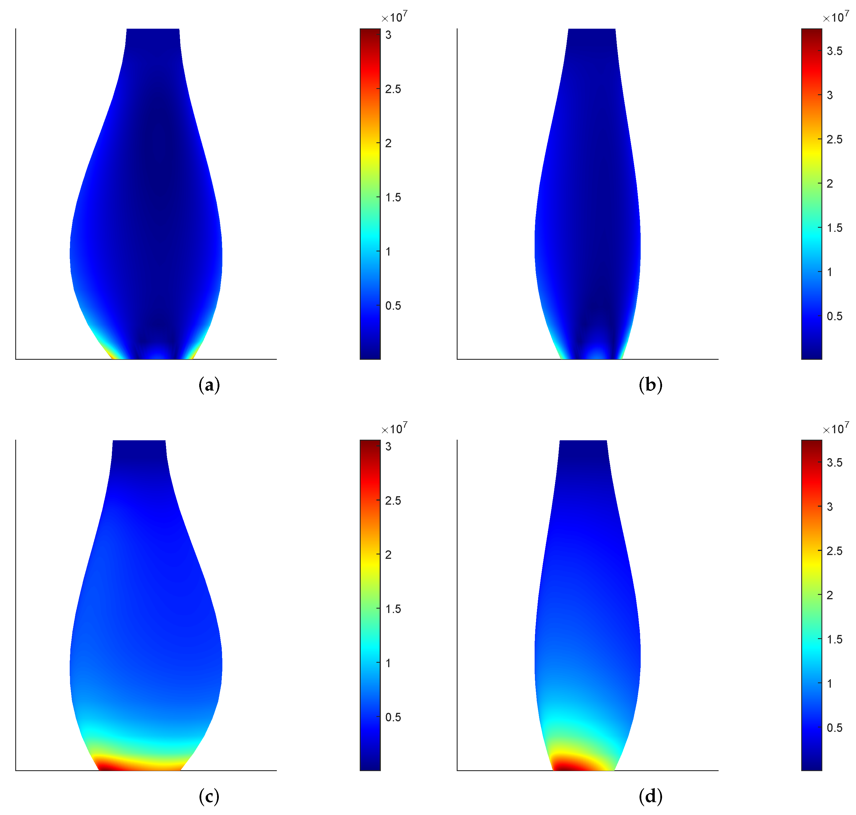
The von Mises stress for each airfoil point and radius station is calculated using Equation (
15). Due to the aim of keeping the algorithm efficient, the points inside the airfoil are not evaluated because the normal stress has its maximum at the boundary of the cross-section. The results are interpolated and plotted for the optimal propeller by XFOIL and CFD,
Figure 13. The stress distribution is similar for both optimal propellers, where the maximum stress is located at the bottom surface near to the leading edge. It is expected because this section is under tension by drag, lift, and centrifugal force, while the top surface has a low von Mises stress because this section is under compression by lift counterweighted by the tension of centrifugal force.
The implemented structural methodology is compared against the FEA method to validate the results. Additionally, the same CFD propeller and operational condition of
Figure 13 are analyzed without centrifugal force to conclude its impact. Finally, the FEA mesh is shown in
Figure 14. The root of the propeller is clamped, and each axial and tangential force from the BEMT sections is set in the respective radius positions at the FEA model, where the aerodynamic forces are assumed to be located at 0.25 of the airfoil chord.
The comparison between FEA and the implemented method is shown in
Figure 15. The stress distribution is almost the same along the blade, with a relative error of 11.7% for the maximum stress value. Additionally, the distribution and maximum stress value without the centrifugal force of 1.8 × 10
Pa are significantly lower than 3 × 10
Pa of
Figure 13 where centrifugal force was considered. Both the high rotational speed of the propeller and the fact that the thrust is low makes the centrifugal force meaningful at this kind of propeller.
7.3. Wind Tunnel Tests and Manufacture
The propellers were printed using the rigid 10 K resin from formlabs. The manufacturer reported data in which the isotropy for this stereolithography (SLA) is proved; hence, the structural model implemented is suitable for resin printed parts. Moreover, the Young modulus of
prevents the performance alteration by the tip deflection, a phenomenon that is not considered at the BEMT. The printed propellers and the motor test stand can be shown in
Figure 16.
The wind tunnel employed is an open circuit type with a testing section of 60 cm wide, 40 cm high, and 140 cm long. The maximum airspeed at the testing section is 42 m/s with a power of 18 kW. The airspeed is estimated by a pitot probe where a dynamic pressure sensor is employed to measure the atmospheric and static pressure, and a thermocouple gauge measures the temperature. These data are used to estimate the air density inside the testing section. The instrument employed for thrust measurement is a force gauge LUTRON FG-20KG with an uncertainty of ±0.01 N. The rotational speed is measured with the optical tachometer PCE-DT62 with an uncertainty of ±1 RPM. Finally, the torque is calculated using Equation (
3), where the current is measured by a clamp meter with an uncertainty of ±0.1 A.
Wind tunnel tests were carried out at the operation point for both CFD and XFOIL optimal propellers. The force gauge employed measures the thrust minus the motor test stand drag, hence a correction of the raw data using the classical momentum theory assumptions is used. Considering Equations (
28) and (
29), the real thrust can be estimated by an iterative process.
Table 2 shows the experimental results and their comparison against the theoretical values from the implemented methods. The results are compared using the coefficients due to the difference in the air density at the optimization routine and the test conditions. The error in torque (or current) is higher than thrust for both CFD and XFOIL propellers, caused by the higher error in drag prediction in comparison to the lift. Nevertheless, the error for the optimal propeller by BEMT-OpenFOAM is considerably lower than the XFOIL one. Moreover, the CFD propeller also has an experimental efficiency
of
higher than XFOIL.
The optimal CFD propeller has a diameter of 0.2946 m and a nominal pitch (at 0.75R) of 0.2362 m and operational condition of
with a respective experimental
and
. The closer commercial propeller with experimental data available is the APC 11X10 (0.2794 m of diameter and 0.254 m of pitch) [
3] with an efficiency of
at the same
J (the maximum efficiency is
at a bit higher
J value), but with a considerable lower
. If the comparison is made at the same thrust coefficient, the commercial propeller efficiency is
.
8. Future Work
Several improvements can be considered for the optimization method. First, although the BEMT shows promising results when corrections are applied, it is not as accurate as a high-fidelity CFD simulation of the whole propeller. The problem is the extremely high computational cost it would require. The use of high-performance computers working in parallel combined with an optimized CFD routine for propeller analysis would allow the optimization routine to use 3D CFD simulations instead of BEMT coupled with airfoil simulations, resulting in more accurate optimized designs that would not require further analysis and refinement (rotational corrections). Additionally, a second-order DC electric motor model (non-constant resistance, non-constant no-load current, and other non-linear effects) can be implemented and the results compared.
The method works for larger propellers, but the coefficients for the rotational corrections would require more investigation and fitting. Moreover, a different turbulence model could be required for different Reynolds regimes. In order to reduce the computational effort, the OpenFOAM routine should run with parallel processing at meshing and solving, including a pseudo-transient method, which was not implemented.
Multi-objective optimization can be implemented straightforwardly using the weighted method, being this trade-off function the objective of the PSO. Additionally, other optimization methods such as a grey wolf [
46] or whale optimizer [
47] can be compared against PSO. Moreover, a noise model can be considered in the optimization, despite the fact that the tested propellers were not considerably noisy.
Finally, the structural model proved its suitability as a trade-off between accuracy and computational cost for the propellers but was unable to cope with anisotropic materials, which is not an issue for SLA printing or aluminum, but it would be a problem for wooden or carbon fiber propellers. Moreover, propellers made of composite materials can take advantage of coupling effects to have different pitch distribution at different flight conditions (and loads), being optimal at different flight stages or missions. The latter will require a fast algorithm to predict the complex behavior of anisotropic composites.
9. Conclusions
The aero-structural optimization carried out by the constrained PSO proved to be a feasible solution in propeller design. A BEMT model showed accurate results throughout the propeller prediction process, and the proposed improvement in convergence reduces the computational cost. Moreover, a study on the number of blade sections in BEMT showed to be relevant for predicting the propeller performance in the minimum time. The BEMT model fed by OpenFOAM had a considerably lower error in thrust and torque predictions than XFOIL, being the thrust more accurate than torque. These BEMT-CFD results, considering the corrections employed and suggested, have similar accuracy to the 3D propeller CFD results.
The difficulties in convergence for some airfoil shapes and the Reynolds regime required implementing the drag coefficient correction based on the Reynolds. Moreover, a similar approach for the stall angle was proposed and successfully implemented in the propeller optimization using experimental data of NACA airfoils.
A study case was carried out for a specific target thrust, operational conditions, and motor. The CFD and XFOIL optimal propellers were printed by stereolithography and tested in the wind tunnel. The error of the XFOIL propeller is considerably high in torque and thrust, while the CFD propeller had a good fitting, with the torque error being higher than the thrust for both methods, which suggests further research to improve drag prediction. Additionally, from the experimental test, the CFD propeller achieved a higher efficiency of than XFOIL, where XFOIL did not reach the target thrust at the expected conditions.
Moreover, the optimal CFD blade was compared against a commercial propeller with the same diameter and pitch. If the comparison is made at the same advance ratio J, the CFD propeller has higher efficiency and higher thrust. On the other hand, if the comparison is made at the same thrust, the CFD propeller has a higher efficiency.
The optimal pitch distribution was monotonically decreasing, while the chord increased and decreased, suggesting a larger chord where the Reynolds is at the maximum. The optimal chord and pitch distributions of BEMT-PSO were compared to the optimal vortex solution (Goldstein). The vortex chord is shorter and the pitch is higher, which probably means the non-compliance of structural constraints. Nevertheless, the pitch shape from the vortex optimization is quite similar to BEMT-PSO but with a constant offset ( for the study case), especially for the CFD propeller. The latter means that the pitch distribution can be modeled as the Goldstein solution plus a constant parameter, which considerably reduces the number of parameters to be optimized in the process and, consequently, the computational cost. The pitch of XFOIL and CFD are also very similar in shape and values, with the chord distribution being the main difference. The latter probably means that the CFD and XFOIL prediction for the angle of best lif-to-drag ratio is very similar, but the value of the lift and drag at this angle is not.
The airfoil shape distribution of XFOIL and CFD showed a minimum thickness at the middle of the blade where the maximum Reynolds number is reached, and a minimum camber in some radius between tip and hub. In addition, the camber distributions have their local maximums at the lowest chord values where the Reynolds number is the minimum, suggesting an optimal lift distribution. The camber distribution of CFD and XFOIL has the same value about the middle of the blade, where predictions of CFD and XFOIL are more similar due to the higher Reynolds. Moreover, the maximum camber position increases linearly for the CFD propeller with conservative values about 0.45 of the chord, keeping a smooth airfoil surface that prevents boundary layer separation. On the other hand, XFOIL has a more aggressive curve at the beginning of the airfoil surface, probably because of its accuracy stall and drag prediction limitations.
The Euler–Bernoulli beam theory was successfully applied to estimate the Von Mises stress, which showed similar results compared to Finite Element Analysis, being a suitable trade-off between accuracy and computational cost. Moreover, the centrifugal force at the propeller was meaningful, which rejects the idea of neglecting it, especially for small-sized propellers. Finally, the feasibility of the printed propellers was proved, and the stereolithography’s isotropic behavior allows the use of simple stress estimation methods. The general workflow also works for anisotropic materials, but another stress estimation methodology must be employed with another failure criterion such as Tsai–Hill or Tsai–Wu.
Author Contributions
Conceptualization, J.D.H. and J.H.J.; methodology, J.D.H., J.H.J. and C.E.; software, J.D.H., J.H.J. and C.E.; validation, J.D.H., J.H.J. and C.E.; formal analysis, J.D.H., J.H.J. and C.E.; investigation, J.D.H., C.E. and J.P.A.; resources, J.P.A. and G.U.; data curation, J.H.J. and C.E.; writing—original draft preparation, J.D.H.; writing—review and editing, J.H.J., C.E., J.P.A. and G.U.; visualization, J.P.A. and G.U.; supervision, J.P.A. and G.U.; project administration, J.D.H. and J.P.A.; funding acquisition, J.P.A. and G.U. All authors have read and agreed to the published version of the manuscript.
Funding
This research was partially funded by Boeing.
Institutional Review Board Statement
Not applicable.
Informed Consent Statement
Not applicable.
Data Availability Statement
The data that support the findings of this study are available from the corresponding authors upon reasonable request.
Acknowledgments
The authors thank Boeing again for its financial support.
Conflicts of Interest
The authors declare no conflict of interest.
Nomenclature
| A | cross-section area |
| propeller disk area |
| B | number of blades |
| motor stand drag coefficient |
| propeller torque coefficient |
| propeller thrust coefficient |
| drag force per length unit |
| motor stand drag |
| drag considering propeller wake |
| Prandt’s tip-loss factor |
| centrifugal force |
| tangential force component per length unit |
| axial force component per length unit |
| vector with best design variables by any particle |
| inertia around the x-axis |
| inertia around the y-axis |
| J | advance ratio |
| motor torque constant |
| motor speed constant |
| lift force per length unit |
| vector with best design the individual particle has reached |
| M | Mach number |
| bending moment around centroidal x-axis (assumed parallel to the chord line) |
| bending moment around centroidal y-axis |
| electrical power |
| shaft power |
| R | total blade radius |
| motor electrical resistance |
| Reynolds number |
| reference Reynolds number |
| ESC resistance |
| hub radius |
| random variable between 0 and 1 |
| random variable between 0 and 1 |
| S | reference area |
| T | propeller thrust |
| torsional moment |
| Q | propeller torque |
| relative velocity |
| particle speed at time t |
| free stream speed |
| particle position at time t |
| a | coefficient of rotational correction |
| b | coefficient of rotational correction |
| axial induction factor |
| c | chord |
| lift coefficient |
| uncorrected lift coefficient |
| three-dimensional corrected lift coefficient |
| drag coefficient |
| uncorrected lift coefficient |
| three-dimensional corrected lift coefficient |
| local axial force coefficient |
| d | propeller diameter |
| h | coefficient of rotational correction |
| i | current |
| no-load current |
| n | revolutions per second |
| r | radius |
| local radius |
| t | thickness |
| v | electric motor terminal voltage |
| velocity induced by propeller |
| back electromotive force |
| tangential component of induced velocity |
| axial component of induced velocity |
| x | x-coordinate of any point inside airfoil with respect to its centroid |
| airfoil position of maximum camber in chord percentage |
| y | y-coordinate of any point inside airfoil with respect to its centroid |
| z | airfoil maximum camber in chord percentage |
| revolutions per second |
| angle of attack |
| Stall angle |
| safety factor |
| electrical efficiency |
| propeller efficiency |
| total efficiency |
| local pitch |
| convenience factor for induced velocity calculation |
| weight factor |
| air density |
| material density |
| normal stress |
| von Mises stress |
| yield tensile strength |
| maximum shear stress |
| inflow angle |
| constant describing how strong the best global solution attracts the particle |
| constant describing how strong the best individual particle solution attracts the particle |
| solidity factor |
| Subscripts |
| cen | centroid |
| quarter chord location |
References
- Balaram, J.; Aung, M.; Golombek, M. The Ingenuity Helicopter on the Perseverance Rover. Space Sci. Rev. 2021, 217, 56. [Google Scholar] [CrossRef]
- Gur, O.; Rosen, A. Optimization of Propeller Based Propulsion System. J. Aircr. 2009, 46, 95–106. [Google Scholar] [CrossRef]
- Brandt, J.; Deters, R.; Ananda, G.; Selig, M. UIUC Propeller Database. 2015. Available online: http://m-selig.ae.illinois.edu/props/propDB.html (accessed on 15 February 2020).
- Park, D.; Lee, Y.; Cho, T.; Kim, C. Design and Performance Evaluation of Propeller for Solar-Powered High-Altitude Long-Endurance Unmanned Aerial Vehicle. Int. J. Aerosp. Eng. 2018, 2018, 5782017. [Google Scholar] [CrossRef]
- Liu, S.; Janajreh, I. Development and application of an improved blade element momentum method model on horizontal axis wind turbines. Int. J. Energy Environ. Eng. 2012, 3, 30. [Google Scholar] [CrossRef] [Green Version]
- Vesting, F.; Bensow, R.E. Particle swarm optimization: An alternative in marine propeller optimization? Eng. Optim. 2018, 50, 70–88. [Google Scholar] [CrossRef]
- Mirjalili, S.; Lewis, A.; Mirjalili, S.A.M. Multi-objective Optimisation of Marine Propellers. Procedia Comput. Sci. 2015, 51, 2247–2256. [Google Scholar] [CrossRef] [Green Version]
- Bacciaglia, A.; Ceruti, A.; Liverani, A. Controllable pitch propeller optimization through meta-heuristic algorithm. Eng. Comput. 2020, 37, 2257–2271. [Google Scholar] [CrossRef]
- Hoyos, J.; Alvarado, J.; Jiménez, J. Propeller aerodynamic optimisation to minimise energy consumption for electric fixed-wing aircraft. Aeronaut. J. 2021, 125, 1844–1870. [Google Scholar] [CrossRef]
- Hoyos, J.D.; Jímenez, J.H.; Echavarría, C.; Alvarado, J.P. Airfoil Shape Optimization: Comparative Study of Meta-heuristic Algorithms, Airfoil Parameterization Methods and Reynolds Number Impact. IOP Conf. Ser. Mater. Sci. Eng. 2021, 1154, 012016. [Google Scholar] [CrossRef]
- Hassan, R.; Cohanim, B.; de Weck, O.; Venter, G. A Comparison of Particle Swarm Optimization and the Genetic Algorithm. In Proceedings of the 46th AIAA/ASME/ASCE/AHS/ASC Structures, Structural Dynamics and Materials Conference, Austin, TX, USA, 18–21 April 2005. [Google Scholar] [CrossRef]
- Goldstein, S. On the Vortex Theory of Screw Propellers. Proc. R. Soc. Math. Phys. Eng. Sci. 1929, 123, 440–465. [Google Scholar]
- Betz, A. Schraubenpropeller mit geringstem Energieverlust. Gott. Nachrichten 1919, 1919, 193–213. [Google Scholar]
- Mian, H.H.; Wang, G.; Zhou, H.; Wu, X. Optimization of thin electric propeller using physics-based surrogate model with space mapping. Aerosp. Sci. Technol. 2021, 111, 106563. [Google Scholar] [CrossRef]
- Hussain, M.; Abdel-Nasser, Y.; Banawan, A.; Ahmed, Y.M. FSI-based structural optimization of thin bladed composite propellers. Alex. Eng. J. 2020, 59, 3755–3766. [Google Scholar] [CrossRef]
- Ning, S.A. A simple solution method for the blade element momentum equations with guaranteed convergence. Wind Energy 2014, 17, 1327–1345. [Google Scholar] [CrossRef]
- Chaviaropoulos, P.; Hansen, M. Investigating Three-Dimensional and Rotational Effects on Wind Turbine Blades by Means of a Quasi3D Navier-Stokes Solver. J. Fluids Eng. 2000, 122, 330–336. [Google Scholar] [CrossRef]
- Bak, C.; Johansen, J.; Andersen, P.B. Three-dimensional corrections of airfoil characteristics based on pressure distributions. In Proceedings of the European Wind Energy Conference, Athens, Greece, 22 February–2 March 2006; pp. 1–10. [Google Scholar]
- Hansen, M.O.; Sørensen, J.N.; Voutsinas, S.; Sørensen, N.; Madsen, H.A. State of the art in wind turbine aerodynamics and aeroelasticity. Prog. Aerosp. Sci. 2006, 42, 285–330. [Google Scholar] [CrossRef]
- Eastman, N.; Jacobs, K.E.W.; Pinkerton, R.M. The Characteristics of 78 Related Airfoil Sections from Tests in the Variable-Density Wind Tunnel; Technical Report; National Advisory Committee for Aeronautics: Washington, DC, USA, 1935. [Google Scholar]
- Alam, M.F.; Thompson, D.S.; KeithWalters, D. Critical Assessment of Hybrid RANS-LES Modeling for Attached and Separated Flows; Konstantin Volko, Turbulence Modelling Approaches: Rijeka, Croatia, 2017. [Google Scholar]
- Montgomerie, B. Methods for Root Effects, Tip Effects and Extending the Angle of Attack to +/−180 with Application to Aerodynamics for Blades on Wind Turbines and Propellers; Technical Report, Swedish Defence Research Agency Scientific Report FOI-R–1305–SE; Bjorn Montgomerie: Stockholm, Switzerland, 2004. [Google Scholar]
- Drela, M. XFOIL: An analysis and design system for low Reynolds number airfoils. In Low Reynolds Number Aerodynamics; Springer: Berlin/Heidelberg, Germany, 1989; pp. 1–12. [Google Scholar]
- Open, C. OpenFOAM user guide. OpenFOAM Found. 2011, 2, U21–U203. [Google Scholar]
- Salim, S.; Cheah, S. Wall y+ strategy for dealing with wall-bounded turbulent flows. In Proceedings of the International MultiConference on Engineerings and Computer Science, Hong Kong, China, 18–20 March 2009. [Google Scholar]
- White, F. Fluid Mechanics, 5th ed.; McGraw-Hill Series in Mechanical Engineering; McGraw Hill: New York, NY, USA, 2003. [Google Scholar]
- Suvanjumrat, C. Comparison of turbulence models for flow past NACA0015 airfoil using OpenFOAM. Eng. J. 2017, 21, 207–221. [Google Scholar] [CrossRef]
- Wang, S.; Ingham, D.B.; Ma, L.; Pourkashanian, M.; Tao, Z. Turbulence modeling of deep dynamic stall at relatively low Reynolds number. J. Fluids Struct. 2012, 33, 191–209. [Google Scholar] [CrossRef]
- Selig, M.S. Summary of Low Speed Airfoil Data; SOARTECH Publications: Champaign, IL, USA, 1995. [Google Scholar]
- Clancy, L. Aerodynamics; Pitman Aeronautical Engineering Series; Wiley: Hoboken, NJ, USA, 1975. [Google Scholar]
- MacNeill, R.; Verstraete, D.; Gong, A. Conference: 53rd AIAA/SAE/ASEE Joint Propulsion Conference Optimisation of Propellers for UAV Powertrains. In Proceedings of the 53rd AIAA/SAE/ASEE Joint Propulsion Conference, Atlanta, GA, USA, 10–12 July 2017. [Google Scholar] [CrossRef]
- Lawrence, D.; Mohseni, K. Efficiency Analysis for Long Duration Electric MAVs. In Infotech@Aerospace; AIAA: Arlington, VA, USA, 2012. [Google Scholar] [CrossRef]
- Mccrink, M.; Gregory, J. Blade Element Momentum Modeling of Low-Reynolds Electric Propulsion Systems. J. Aircr. 2016, 54, 1–14. [Google Scholar] [CrossRef]
- Sodja, J.; Drazumeric, R.; Kosel, T.; Marzocca, P. Design of Flexible Propellers with Optimized Load-Distribution Characteristics. J. Aircr. 2014, 51, 117–128. [Google Scholar] [CrossRef]
- Epps, B.; Ketcham, J.; Chryssostomidis, C. Propeller Blade Stress Estimates Using Lifting Line Theory. In Proceedings of the 2010 Conference on Grand Challenges in Modeling and Simulation (GCMS ’10), Ottawa, ON, Canada, 11–14 July 2010; Society for Modeling and Simulation International: Vista, CA, USA, 2010; pp. 442–447. [Google Scholar]
- Pourrajabian, A.; Nazmi Afshar, P.A.; Ahmadizadeh, M.; Wood, D. Aero-structural design and optimization of a small wind turbine blade. Renew. Energy 2016, 87, 837–848. [Google Scholar] [CrossRef]
- Young, W.; Budynas, R.; Sadegh, A. Roark’s Formulas for Stress and Strain, 8th ed.; McGraw-Hill Education: Manhattan, NY, USA, 2011. [Google Scholar]
- Glauert, H. The Elements of Aerofoil and Airscrew Theory; Cambridge Science Classics; Cambridge University Press: Cambridge, UK, 1983. [Google Scholar] [CrossRef]
- Jiménez, J.H.; Hoyos, J.D.; Echavarría, C.; Alvarado, J.P. Exhaustive Analysis on Aircraft Propeller Performance through a BEMT Tool. J. Aeronaut. Astronaut. Aviat. 2022, 54, 13–23. [Google Scholar]
- von Karman, T. Compressibility Effects in Aerodynamics. J. Aeronaut. Sci. 1941, 8, 337–356. [Google Scholar] [CrossRef]
- Tsien, H.S. Two-Dimensional Subsonic Flow of Compressible Fluids. J. Aeronaut. Sci. 1939, 6, 399–407. [Google Scholar] [CrossRef]
- Sriti, M. Improved Blade Element Momentum theory (BEM) for Predicting the Aerodynamic Performances of Horizontal Axis Wind Turbine Blade (HAWT). Tech.-Mech.-Eur. J. Eng. Mech. 2018, 38, 191–202. [Google Scholar]
- Hernández, J.; Crespo, A. Aerodynamic Calculation of the Performance of Horizontal Axis Wind Turbines and Comparison with Experimental Results. Wind Eng. 1987, 11, 177–187. [Google Scholar]
- Sheldahl, R.E.; Klimas, P. Aerodynamic Characteristics of Seven Symmetrical Airfoil Sections through 180-Degree Angle of Attack for Use in Aerodynamic Analysis of Vertical Axis Wind Turbines; Technical Report; Sandia National Laboratories—Energy Report Sandia National Labs.: Albuquerque, NM, USA, 1981.
- Parsopoulos, K.E.; Vrahatis, M.N. Particle Swarm Optimization and Intelligence: Advances and Applications; Information Science Publishing (IGI Global): Hershey, PA, USA, 2010. [Google Scholar] [CrossRef]
- Mirjalili, S.; Mirjalili, S.M.; Lewis, A. Grey Wolf Optimizer. Adv. Eng. Softw. 2014, 69, 46–61. [Google Scholar] [CrossRef] [Green Version]
- Mirjalili, S.; Lewis, A. The Whale Optimization Algorithm. Adv. Eng. Softw. 2016, 95, 51–67. [Google Scholar] [CrossRef]
Figure 1.
Grid independence and computational time for C-grid topology. Lift coefficient (a) and drag coefficient (b).
Figure 1.
Grid independence and computational time for C-grid topology. Lift coefficient (a) and drag coefficient (b).
Figure 2.
C-grid topology with cells from far view (a) and close view (b).
Figure 2.
C-grid topology with cells from far view (a) and close view (b).
Figure 3.
Wind tunnel data, CFD OpenFOAM and Xfoil lift coefficients and drag coefficients validation for a , , .
Figure 3.
Wind tunnel data, CFD OpenFOAM and Xfoil lift coefficients and drag coefficients validation for a , , .
Figure 4.
DC motor equivalent circuit (adapted from [
31]).
Figure 4.
DC motor equivalent circuit (adapted from [
31]).
Figure 6.
Percentual relative difference of thrust coefficient and efficiency against number of blade sections.
Figure 6.
Percentual relative difference of thrust coefficient and efficiency against number of blade sections.
Figure 7.
Validation of (a) and (b).
Figure 7.
Validation of (a) and (b).
Figure 8.
Flowchart of the optimization.
Figure 8.
Flowchart of the optimization.
Figure 9.
PSO iterations of the total efficiency for CFD and XFOIL propellers.
Figure 9.
PSO iterations of the total efficiency for CFD and XFOIL propellers.
Figure 10.
Comparison of optimal propeller by XFOIL and CFD and its respective Goldstein optimization for pitch (a) and chord distribution (b).
Figure 10.
Comparison of optimal propeller by XFOIL and CFD and its respective Goldstein optimization for pitch (a) and chord distribution (b).
Figure 11.
Distribution of maximum thickness (a) and maximum camber z (b) along optimal CFD and XFOIL blade.
Figure 11.
Distribution of maximum thickness (a) and maximum camber z (b) along optimal CFD and XFOIL blade.
Figure 12.
Distribution of maximum camber position along optimal CFD and XFOIL blade.
Figure 12.
Distribution of maximum camber position along optimal CFD and XFOIL blade.
Figure 13.
Von Mises stress predicted (Pa) on the optimal CFD propeller considering centrifugal force by the implemented method, top (a) and bottom view (c), and optimal XFOIL propeller, top (b) and bottom view (d).
Figure 13.
Von Mises stress predicted (Pa) on the optimal CFD propeller considering centrifugal force by the implemented method, top (a) and bottom view (c), and optimal XFOIL propeller, top (b) and bottom view (d).
Figure 14.
Finite Element Analysis mesh.
Figure 14.
Finite Element Analysis mesh.
Figure 15.
Von Mises stress (Pa) predicted on the optimal CFD propeller without considering centrifugal force by the implemented method, top (a) and bottom view (c), and Finite Element Analysis results by CATIA V5, top (b) and bottom view (d).
Figure 15.
Von Mises stress (Pa) predicted on the optimal CFD propeller without considering centrifugal force by the implemented method, top (a) and bottom view (c), and Finite Element Analysis results by CATIA V5, top (b) and bottom view (d).
Figure 16.
Motor test stand and the wind tunnel (a) and printed propellers (b).
Figure 16.
Motor test stand and the wind tunnel (a) and printed propellers (b).
Table 1.
Data and constraints for the optimization.
Table 1.
Data and constraints for the optimization.
| () | (m) | T (N) | () | | | | |
|---|
| 0.02 | 55.5015 | 0.30 | 20 | 15 | 25 | 1.9 | 60 | 1.5 |
Table 2.
Experimental results.
Table 2.
Experimental results.
| | | | | | error | error | |
|---|
| XFOIL | 0.0768 | 0.0946 | 0.005286 | 0.006955 | 18.81% | 23.99% | 72.30% |
| CFD | 0.0994 | 0.1012 | 0.006453 | 0.006716 | 1.77% | 3.92% | 79.26% |
| Publisher’s Note: MDPI stays neutral with regard to jurisdictional claims in published maps and institutional affiliations. |
© 2022 by the authors. Licensee MDPI, Basel, Switzerland. This article is an open access article distributed under the terms and conditions of the Creative Commons Attribution (CC BY) license (https://creativecommons.org/licenses/by/4.0/).

 ,
, 


