
Discrete-Time Attitude Tracking Synchronization for Swarms of Spacecraft Exploiting Interference


Abstract
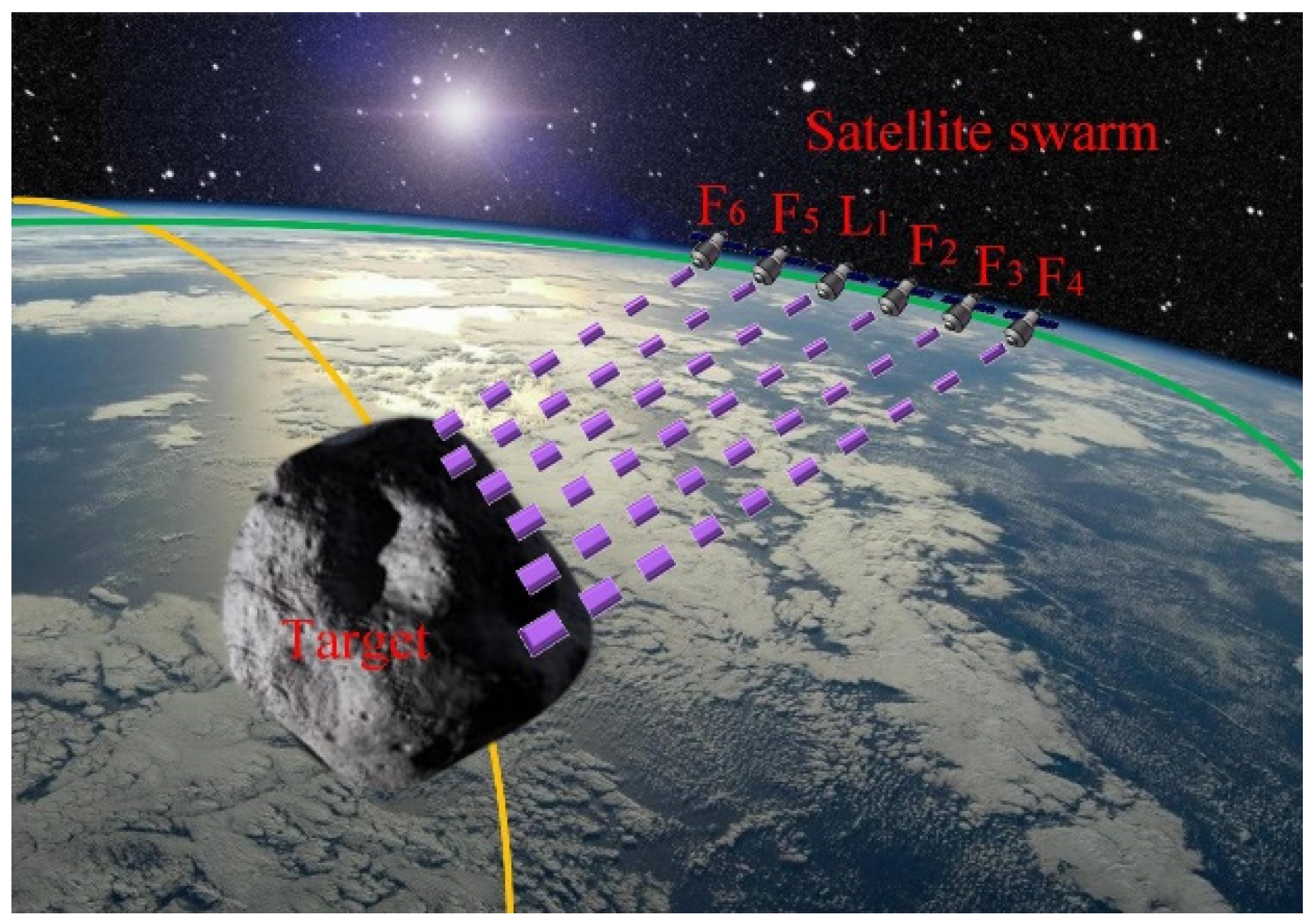
:1. Introduction
2. Problem Description and Preliminary Knowledge
2.1. Kinematics and Dynamics
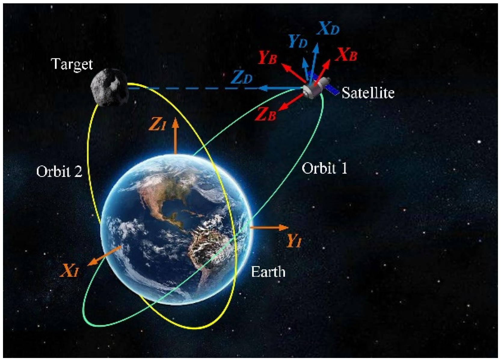
2.1.1. Axis Frame
- Earth Centered Inertial Frame, . The origin of is fixed to the barycenter of the Earth. The plane coincides with the equatorial plane. The axis points to the North Pole, the axis points to the vernal equinox and the axis is determined according to the right-hand rule.
- Spacecraft Body Fixed Frame, . It is fixed on the spacecraft, and the frame origin corresponds to the center of mass. The axis points along the longitudinal axis of the spacecraft. The axis and the axis lie, respectively, along the other two principal axes of the spacecraft according to the right-hand rule.
- Desired Imaging Frame, . The origin of corresponds to the center of mass of the spacecraft. The axis points to the target. The axis is determined by , where and are the unit vectors of the axis and the axis. Then the axis is determined according to the right-hand rule.
2.1.2. Quaternion Kinematics
2.1.3. Attitude Dynamics
2.1.4. Orbit Elements
- Calculate the orbital period : ,
- Calculate the mean anomaly : ,
- Calculate the eccentric anomaly by solving the Kepler equation: ,
- Calculate the true anomaly : ,
- Calculate the distance between the barycenter of the target and the barycenter of the Earth : ,
- Calculate : , where
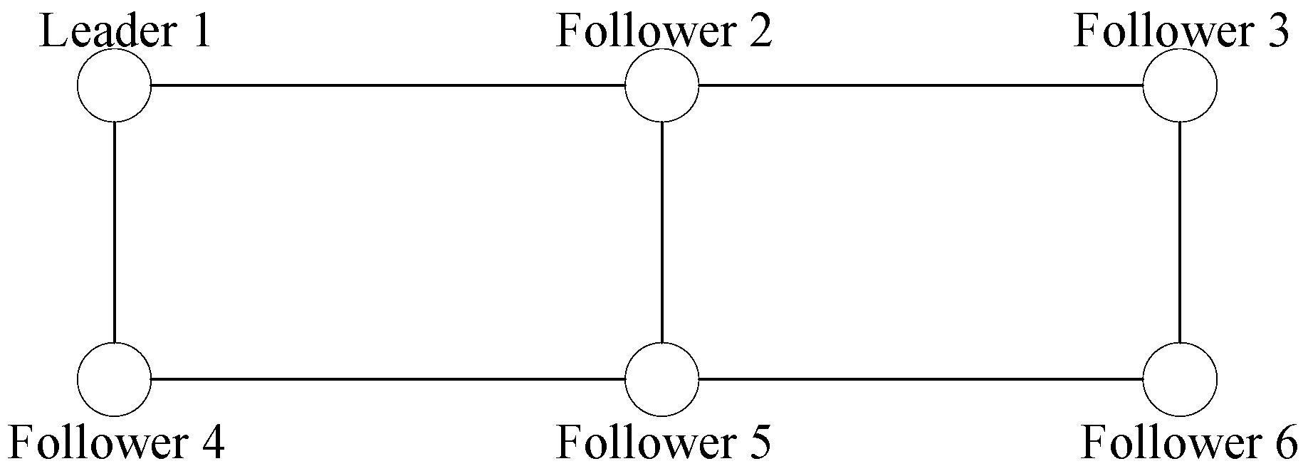
2.2. Graph
2.3. The Model for Wireless Interference
2.4. Stabilization Theory of Sampled-Data Nonlinear Systems
- ,
- ,
- There exist,,and for each,such that, we haveand.
- For each compact set there existandsuch that, and,
2.5. The Mathematic Model of Problem Description
3. Control Law Design
3.1. Attitude Determination of the Virtual Leader Spacecraft
3.2. Communication System Exploiting Interference
3.3. Design of Attitude Tracking Synchronization Control Scheme
3.3.1. Continuous Control Scheme
3.3.2. Discrete Control Scheme
- , where,
- ,where .
- ii.
- should be positive definite . Which means, by choosing and to satisfyis ensured to be positive definite .
- iii.
- Defineaccording to Lemma 7,should be guaranteed. With some calculationswhere
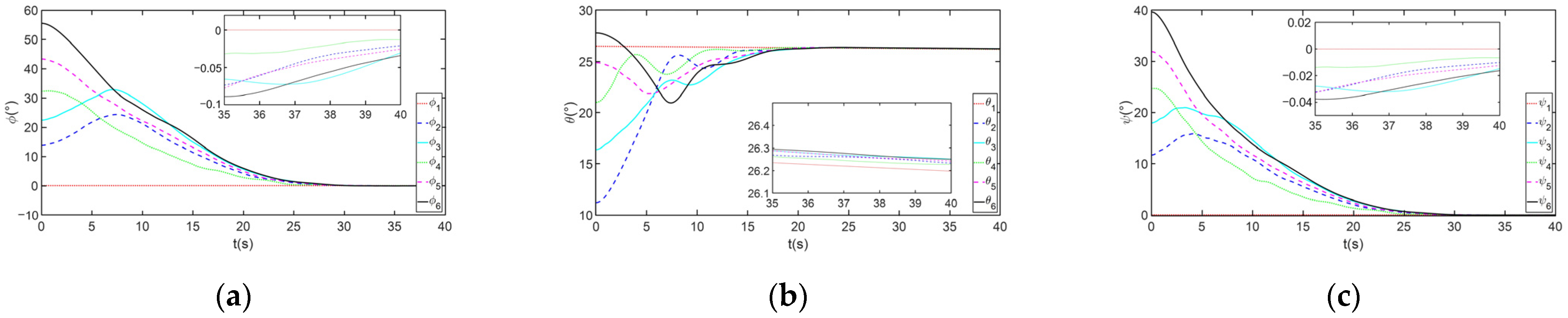
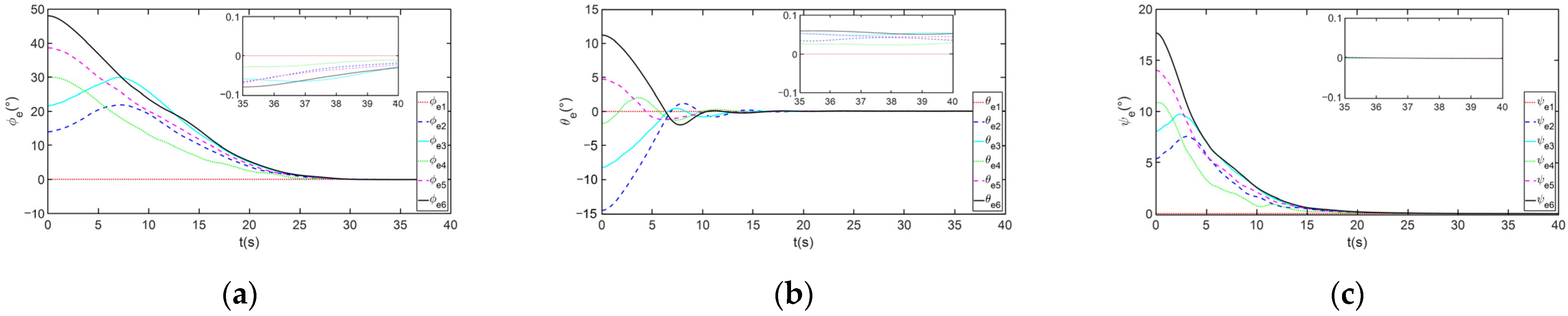
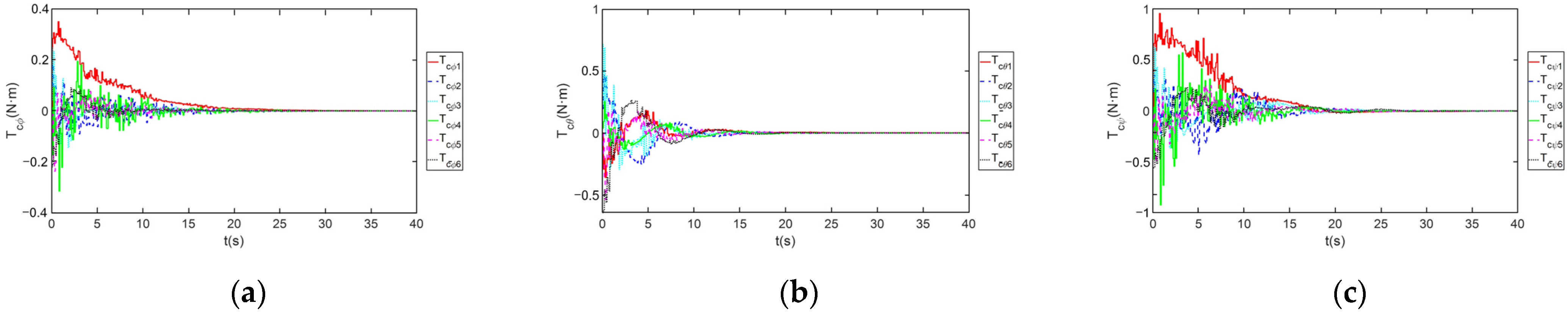
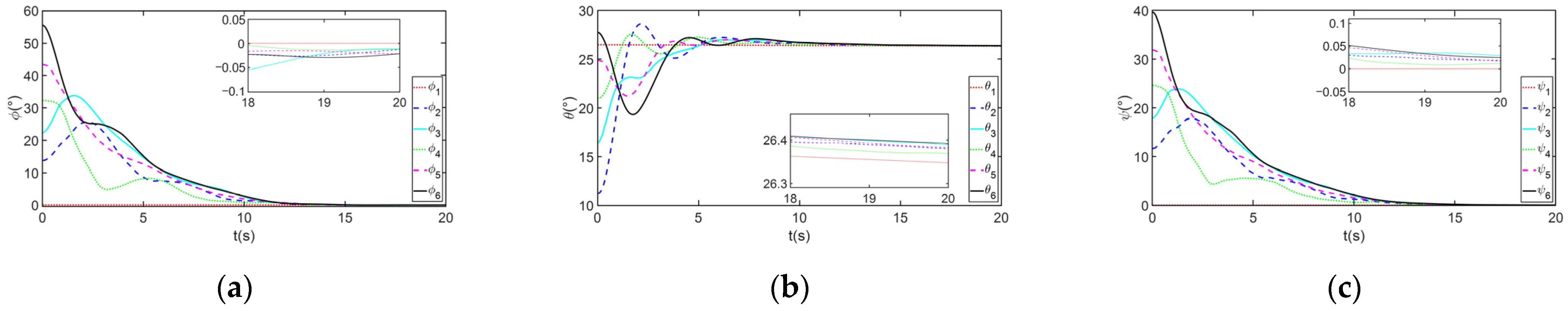
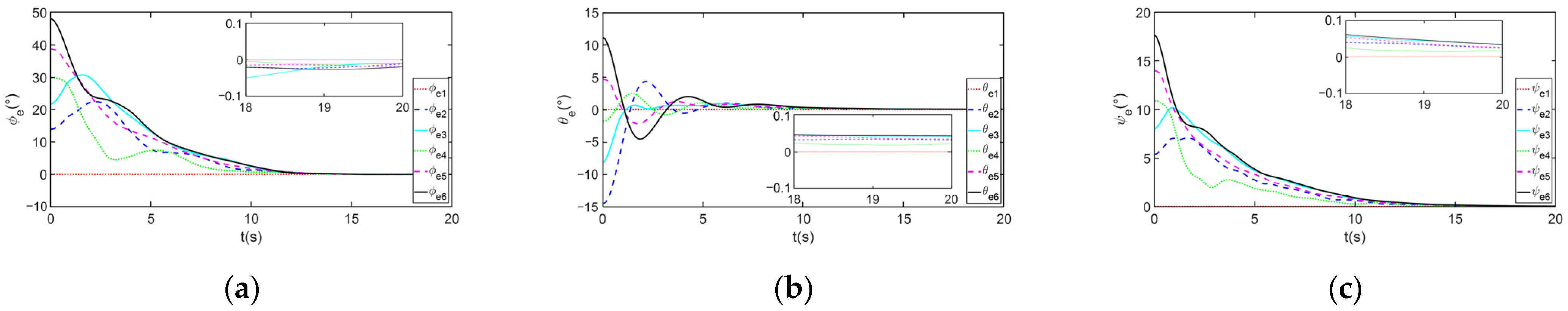
4. Simulation Results
4.1. The Control Case Utilizing Liquid Propulsion (LP) Systems
4.2. The Control Case Utilizing Solid Rocket Propulsion (SRP) Systems or Nuclear Propulsion (NP) Systems
5. Conclusions
Author Contributions
Funding
Institutional Review Board Statement
Informed Consent Statement
Data Availability Statement
Conflicts of Interest
References
- Nosseir, A.E.S.; Cervone, A.; Pasini, A. Modular impulsive green monopropellant propulsion system (mimps-g): For cubesats in leo and to the moon. Aerospace 2021, 8, 169. [Google Scholar] [CrossRef]
- Kramer, A.; Bangert, P.; Schilling, K. Uwe-4: First electric propulsion on a 1u cubesat in-orbit experiments and characterization. Aerospace 2020, 7, 98. [Google Scholar] [CrossRef]
- Bandyopadhyay, S.; Foust, R.; Subramanian, G.P.; Chung, S.-J.; Hadaegh, F.Y. Review of formation flying and constellation missions using nanosatellites. J. Spacecr. Rocket. 2016, 53, 567–578. [Google Scholar] [CrossRef] [Green Version]
- Utschick, W. Communications in Interference Limited Networks; Springer: Cham, Switzerland, 2016. [Google Scholar]
- Truszkowski, W.; Hinchey, M.; Rash, J.; Rouff, C. NASA’s swarm missions: The challenge of building autonomous software. IT Prof. 2004, 6, 47–52. [Google Scholar] [CrossRef]
- Liu, H.; Xie, G.; Wang, L. Necessary and sufficient conditions for containment control of networked multi-agent systems. Automatica 2012, 48, 1415–1422. [Google Scholar] [CrossRef]
- Borzone, T.; Morărescu, I.-C.; Jungers, M.; Boc, M.; Janneteau, C. Hybrid framework for consensus in fleets of non-holonomic robots. In Proceedings of the 2018 Annual American Control Conference (ACC), Milwaukee, WI, USA, 27–29 June 2018; pp. 4299–4304. [Google Scholar]
- Chen, Z.; Chen, X. Robust sampled-data output synchronization of nonlinear heterogeneous multi-agents. IEEE Trans. Autom. Control 2016, 62, 1458–1464. [Google Scholar] [CrossRef]
- Abdessameud, A.; Tayebi, A.; Polushin, I.G. Leader-follower synchronization of euler-lagrange systems with time-varying leader trajectory and constrained discrete-time communication. IEEE Trans. Autom. Control 2016, 62, 2539–2545. [Google Scholar] [CrossRef]
- Furieri, L.; Kamgarpour, M. The value of communication in designing robust distributed controllers. arXiv 2017, arXiv:1711.05324. [Google Scholar]
- Olfati-Saber, R.; Fax, J.; Murray, R. Consensus and cooperation in networked multi-agent systems. Proc. IEEE 2007, 95, 215–233. [Google Scholar] [CrossRef] [Green Version]
- Mei, J.; Ren, W.; Chen, J.; Ma, G. Distributed adaptive coordination for multiple lagrangian systems under a directed graph without using neighbors velocity information. Automatica 2013, 49, 1723–1731. [Google Scholar] [CrossRef]
- Zhao, S.; Zelazo, D. Bearing rigidity and almost global bearing-only formation stabilization. IEEE Trans. Autom. Control 2015, 61, 1255–1268. [Google Scholar] [CrossRef] [Green Version]
- Ren, W.; Beard, R.W.; Atkins, E.M. Information consensus in multivehicle cooperative control. IEEE Control Syst. Mag. 2007, 27, 71–82. [Google Scholar]
- Jie, M.; Wei, R.; Jie, C.; Anderson, B.D.O. Consensus of linear multi-agent systems with fully distributed control gains under a general directed graph. In Proceedings of the 53rd IEEE Conference on Decision and Control, Los Angeles, CA, USA, 15–17 December 2014; pp. 2993–2998. [Google Scholar]
- Movric, K.H.; Lewis, F.L. Cooperative optimal control for multi-agent systems on directed graph topologies. IEEE Trans. Autom. Control 2014, 59, 769–774. [Google Scholar] [CrossRef]
- Lewis, F.L.; Cui, B.; Ma, T.; Song, Y.; Zhao, C. Heterogeneous multi-agent systems: Reduced-order synchronization and geometry. IEEE Trans. Autom. Control 2016, 61, 1391–1396. [Google Scholar] [CrossRef]
- Ren, W. Distributed leaderless consensus algorithms for networked euler–lagrange systems. Int. J. Control 2009, 82, 2137–2149. [Google Scholar] [CrossRef]
- Chen, L.-M.; Li, C.-J.; Mei, J.; Ma, G.-F. Adaptive cooperative formation-containment control for networked euler–lagrange systems without using relative velocity information. IET Control Theory Appl. 2017, 11, 1450–1458. [Google Scholar] [CrossRef]
- Du, H.; Li, S. Attitude synchronization for flexible spacecraft with communication delays. IEEE Trans. Autom. Control 2016, 61, 3625–3630. [Google Scholar] [CrossRef]
- Mehrabian, A.; Khorasani, K. Distributed and cooperative quaternion-based attitude synchronization and tracking control for a network of heterogeneous spacecraft formation flying mission. J. Frankl. Inst. 2015, 352, 3885–3913. [Google Scholar] [CrossRef]
- Zhu, Z.; Guo, Y. Adaptive coordinated attitude control for spacecraft formation with saturating actuators and unknown inertia. J. Frankl. Inst. 2019, 356, 1021–1037. [Google Scholar] [CrossRef]
- Yu, Y.; Liu, W.; Yang, Z.; Miao, C.; Jiang, W. A distributed consensus protocol for attitude synchronization and tracking of multiple spacecraft on directed graphs. In Proceedings of the 2019 IEEE 15th International Conference on Control and Automation (ICCA), Edinburgh, UK, 16–19 July 2019; pp. 881–886. [Google Scholar]
- Molinari, F.; Stańczak, S.; Raisch, J. Exploiting the superposition property of wireless communication for max-consensus problems in multi-agent systems. IFAC-PapersOnLine 2018, 51, 176–181. [Google Scholar] [CrossRef]
- Molinari, F.; Stanczak, S.; Raisch, J. Exploiting the superposition property of wireless communication for average consensus problems in multi-agent systems. In Proceedings of the 2018 European Control Conference (ECC), Limassol, Cyprus, 12–15 June 2018; pp. 1766–1772. [Google Scholar]
- Cao, Y.; Yu, W.; Ren, W.; Chen, G. An overview of recent progress in the study of distributed multi-agent coordination. IEEE Trans. Ind. Inform. 2013, 9, 427–438. [Google Scholar] [CrossRef] [Green Version]
- Junkins, J.L.; Schaub, H. Analytical Mechanics of Space Systems; American Institute of Aeronautics and Astronautics: Reston, VA, USA, 2009. [Google Scholar]
- Ickes, B.P. A new method for performing digital control system attitude computations using quaternions. AIAA J. 1970, 8, 13–17. [Google Scholar] [CrossRef]
- Sidi, M.J. Spacecraft Dynamics and Control: A Practical Engineering Approach; Cambridge University Press: Cambridge, UK, 1997; Volume 7. [Google Scholar]
- Xing, Y.; Cao, X.; Zhang, S.; Guo, H.; Wang, F. Relative position and attitude estimation for satellite formation with coupled translational and rotational dynamics. Acta Astronaut. 2010, 67, 455–467. [Google Scholar] [CrossRef]
- Molinari, F.; Raisch, J. Exploiting wireless interference for distributively solving linear equations. IFAC-PapersOnLine 2020, 53, 2999–3006. [Google Scholar] [CrossRef]
- Goldenbaum, M.; Boche, H.; Stańczak, S. Harnessing interference for analog function computation in wireless sensor networks. IEEE Trans. Signal Process. 2013, 61, 4893–4906. [Google Scholar] [CrossRef] [Green Version]
- Nešić, D.; Teel, A.R.; Kokotović, P.V. Sufficient conditions for stabilization of sampled-data nonlinear systems via discrete-time approximations. Syst. Control Lett. 1999, 38, 259–270. [Google Scholar] [CrossRef] [Green Version]
- Arcak, M.; Nešić, D. A framework for nonlinear sampled-data observer design via approximate discrete-time models and emulation. Automatica 2004, 40, 1931–1938. [Google Scholar] [CrossRef]
- Gentle, J.E. Matrix Algebra: Theory, Computations, and Applications in Statistics; Springer Science & Business Media: Berlin/Heidelberg, Germany, 2007. [Google Scholar]
- De Oliveira, M.C. Fundamentals of Linear Control, 1st ed.; Cambridge University Press: Cambridge, UK, 2017; Available online: http://gen.lib.rus.ec/book/index.php?md5=8e37a4532fa49eedf0cde87167a81903 (accessed on 7 June 2020).
- Marshall, A.W.; Olkin, I. Inequalities: Theory of Majorization and Its Applications, 1st ed.; Mathematics in Science and Engineering 143; Academic Press: Cambridge, MA, USA, 1979; Available online: http://gen.lib.rus.ec/book/index.php?md5=0b2ac25bbd5a46c14c037295582b2438 (accessed on 7 June 2020).
- Zhang, F.; Zhang, Q. Eigenvalue inequalities for matrix product. IEEE Trans. Autom. Control 2006, 51, 1506–1509. [Google Scholar] [CrossRef]
- Molinari, F.; Raisch, J. Efficient consensus-based formation control with discrete-time broadcast updates. arXiv 2019, arXiv:1903.07906. [Google Scholar]
- Iserles, A. A First Course in the Numerical Analysis of Differential Equations; Cambridge Texts in Applied Mathematics; Cambridge University Press: Cambridge, UK, 1996; Available online: http://gen.lib.rus.ec/book/index.php?md5=b9acbfe1d21dfcf1aa32e995624f76b1 (accessed on 7 June 2020).
- Wen-Ren, H.K. A sharp upper bound on the largest eigenvalue of the laplacian matrix of a graph. Linear Algebra Appl. 2002, 347, 123–129. [Google Scholar]
- Farrag, A.; Othman, S.; Mahmoud, T.; El Raffiei, A.Y. Satellite swarm survey and new conceptual design for Earth observation applications. Egypt. J. Remote Sens. Space Sci. 2021, 24, 47–54. [Google Scholar] [CrossRef]
- Tummala, A.R.; Dutta, A. An overview of cube-satellite propulsion technologies and trends. Aerospace 2017, 4, 58. [Google Scholar] [CrossRef] [Green Version]
- Wu, Y.H.; Han, F.; Zheng, M.H.; Wang, F.; Hua, B.; Chen, Z.M.; Cheng, Y.H. Attitude tracking control for a space moving target with high dynamic performance using hybrid actuator. Aerosp. Sci. Technol. 2018, 78, 102–117. [Google Scholar] [CrossRef]
- Frisbee, R.H. Limits of interstellar flight technology. Front. Propuls. Sci. 2009, 227, 31–126. [Google Scholar]
- Gibson, M.A.; Mason, L.S.; Bowman, C.L.; Poston, D.I.; McClure, P.R.; Creasy, J.; Robinson, C. Development of NASA’s Small Fission Power System for Science and Human Exploration. In Proceedings of the Joint Propulsion Conference, Cleveland, OH, USA, 28 July 2014. (GRC-E-DAA-TN17266). [Google Scholar]
- Mazouffre, S. Electric propulsion for satellites and spacecraft: Established technologies and novel approaches. Plasma Sources Sci. Technol. 2016, 25, 033002. [Google Scholar] [CrossRef]


| Orbit Elements | Target | Leader 1 | Follower 2 | Follower 3 | Follower 4 | Follower 5 |
|---|---|---|---|---|---|---|
| Semi-major axis a (km) | 6790 | 6900 | 6900 | 6900 | 6900 | 6900 |
| Eccentricity e | 0.0169 | 1 × 10⁻⁹ | 1 × 10⁻⁹ | 1 × 10⁻⁹ | 1 × 10⁻⁹ | 1 × 10⁻⁹ |
| Inclination i (°) | 96 | 30 | 30 | 30 | 30 | 30 |
| Right Ascension of the Ascending Node Ω (°) | 45 | 150 | 150 | 150 | 150 | 150 |
| Argument of Perigee (°) | 30 | 30 | 30 | 30 | 30 | 30 |
| Initial true anomaly Θ0 (°) | 75 | 7 | 7.01 | 7.02 | 7.03 | 6.99 |
Publisher’s Note: MDPI stays neutral with regard to jurisdictional claims in published maps and institutional affiliations. |
© 2022 by the authors. Licensee MDPI, Basel, Switzerland. This article is an open access article distributed under the terms and conditions of the Creative Commons Attribution (CC BY) license (https://creativecommons.org/licenses/by/4.0/).
Share and Cite
Li, P.; Wen, X.; Zheng, M.; Liu, H.; Long, D.; Lu, Y. Discrete-Time Attitude Tracking Synchronization for Swarms of Spacecraft Exploiting Interference. Aerospace 2022, 9, 134. https://doi.org/10.3390/aerospace9030134
Li P, Wen X, Zheng M, Liu H, Long D, Lu Y. Discrete-Time Attitude Tracking Synchronization for Swarms of Spacecraft Exploiting Interference. Aerospace. 2022; 9(3):134. https://doi.org/10.3390/aerospace9030134
Chicago/Turabian StyleLi, Peiran, Xin Wen, Mohong Zheng, Haiying Liu, Dizhi Long, and Yuping Lu. 2022. "Discrete-Time Attitude Tracking Synchronization for Swarms of Spacecraft Exploiting Interference" Aerospace 9, no. 3: 134. https://doi.org/10.3390/aerospace9030134