Autonomous Trajectory Generation Algorithms for Spacecraft Slew Maneuvers

Abstract

Spacecraft need to be able to reliably slew quickly and rather than simply commanding a final angle, a trajectory calculated and known throughout a maneuver is preferred. A fully solved trajectory allows for control based off comparing current attitude to a time varying desired attitude, allowing for much better use of control effort and command over slew orientation. This manuscript introduces slew trajectories using sinusoidal functions compared to optimal trajectories using Pontryagin’s method. Use of Pontryagin’s method yields approximately 1.5% lower control effort compared to sinusoidal trajectories. Analysis of the simulated system response demonstrates that correct understanding of the effect of cross-coupling is necessary to avoid unwarranted control costs. Additionally, a combination of feedforward with proportional derivative control generates a system response with 3% reduction in control cost compared to a Feedforward with proportional integral derivative control architecture. Use of a calculated trajectory is shown to reduce control cost by five orders of magnitude and allows for raising of gains by an order of magnitude. When control gains are raised, an eight orders of magnitude lower error is achieved in the slew direction, and rather than an increase in control cost, a decrease by 11.7% is observed. This manuscript concludes that Pontryagin’s method for generating slew trajectories outperforms the use of sinusoidal trajectories and trajectory generation schemes are essential for efficient spacecraft maneuvering.

1. Introduction

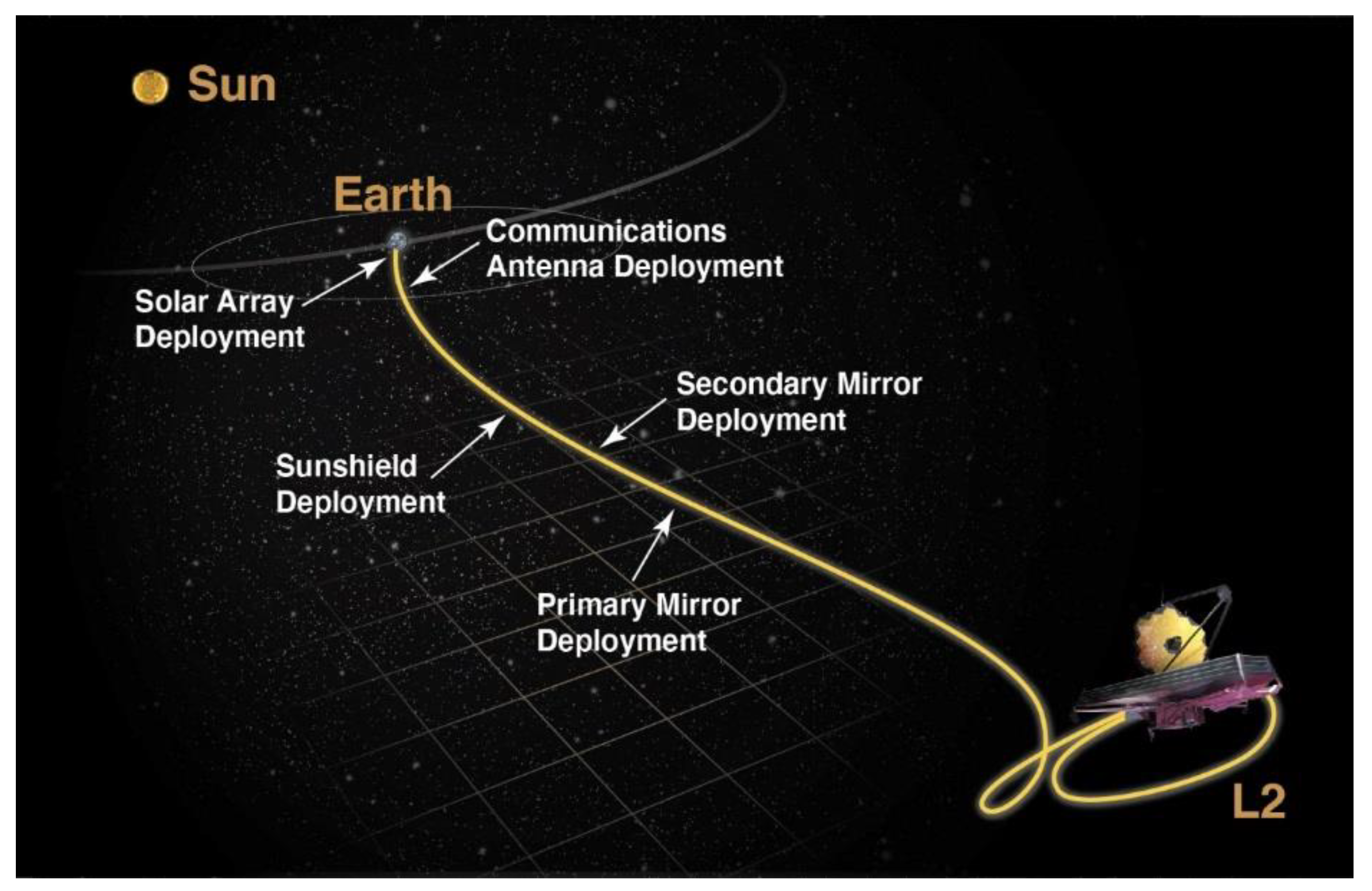
The James Webb telescope depicted in Figure 1 is an example of the paramountcy of attitude trajectories of angular momentum to space mission accomplishment. The James Webb Space telescope (JWST) will study the formation of stars, galaxies, and planets 100–250 million years after the Big Bang. To see the first stars and galaxies of the early universe, JWST must look deep into space, necessitating a need for fine pointing accuracy, one of the reasons JWST is positioned so far away from Earth and the perturbations of the atmosphere. Due to the incredible distance between the JWST and potential imaging targets, pointing errors of mere arcseconds can lead to the telescope field of view not including the intended target, and any spacecraft jitter results in blurry, unusable images. Additionally, the control cost of pointing maneuvers must be considered carefully. Lower control costs result in “cheaper” maneuvers, which can allow for less expensive spacecraft launch, due to mass savings, more possible maneuvers over the spacecraft lifetime due to energy savings, or simply greater error tolerances and recovery capabilities.

The same holds true for near Earth observational satellites. While satellites such as Landsat-9 [3] image targets much closer than JWST does, the increase in magnification power and resolution of such satellites warrants the same need for fine pointing accuracy. Understanding and application of trajectory generation and solution optimality leads to even lower control cost and greater pointing accuracy than has been possible. As pointing accuracy needs increase, attitude trajectories and the provided decrease in pointing error and control cost are vital in making future missions possible.

This manuscript describes two methods of formulating spacecraft attitude slew trajectories and compares various control architectures in performing the generated maneuvers. Rather than the classical formulation of feedback control of a single desired value subtracted from the current state, attention has shifted to more intelligent schemes where the slew trajectory is mapped out for the entire maneuver. Not only does a solved maneuver trajectory allow for more control, customization, and confidence in a control architecture, but also pointing conditions and restraints can be imposed and validated. For example, for a spacecraft to keep a sun-sensor pointed at the sun as best as possible throughout a maneuver. The entire trajectory can be simulated, visualized, and checked ahead of time with a much lower degree of randomness than classical control methods based on final conditions rather than trajectories, might allow. Using trajectories also introduces possibilities for finding optimal solutions, in fuel use, time or distance. One such manner of generating optimal trajectories is by use of Pontryagin’s method. In this manuscript, Pontryagin’s principle of using necessary conditions of optimality to solve for optimal trajectories in terms of control cost will be examined and contrasted with simpler trajectory generation techniques. Additionally, progress has been generated in the development of deterministic artificial intelligence, a control scheme based on a statement of self-awareness, and optimal parameter learning, to determine the optimal control to follow a desired trajectory [4,5,6]. Naturally, the question arises of the effects of applying optimal trajectory optimization methods to such adaptive feedforward methods of optimal control, as well as other control architectures. This manuscript will derive trajectories to perform a given slew maneuver of 30 degrees yaw, as well as present the formalism behind adaptive control techniques and deterministic artificial intelligence. Section 2 describes the materials and methods used to reveal the results presented in Section 3. Section 4 provides a brief discussion on the results in Section 3.

Attitude trajectory adaptation was developed and proposed in [4], but the parameterization suffered from expression in inertial coordinates leading to a high computational burden (thus evaluation of techniques on this basis will remain important). Within just a couple of years, development of the identical technique parameterized in the body frame [5] proved to eliminate a large part of the computational burden. Several years later the burden was reduced still further [6] by 33% and 66% parameter reduction with subsequent experimental validation in [7]. Adaptability is often desirable, but results are sometimes difficult to prove as optimal, minimizing some prescribed cost function. Position and attitude constraints have been simultaneously considered [8] and inherent disturbance rejection as well. Limited control actuation has also been treated [9,10], while optimization has been presented when control moment gyroscopes are used [11], as gyroscope singularity is enormously concerning. Guidance trajectories were derived using only attitude trajectories [12] near small bodies. In 2018, trajectories began to be presented [13] to support the newly proposed deterministic artificial intelligence [14], while at the same time, constrained optimization problems of attitude trajectories were proposed in [15]. Following the former deterministic thread of thinking, deterministic optimal assertion of self-awareness and optimal learning were formulated in [16]. With a renewed focus on attitude trajectory optimization [17], disturbance minimizing trajectories for space robots was just proposed [18]. Finally, convex optimization for trajectory generation [19] was presented amidst a focus on rapid maneuvering agile satellites in constellations [20]. Garcia, et al. [8] highlighted the complicated complexity of optimization of space trajectories generated by the nonlinear, coupled governing equations of motion. Sanyal, et al. [21] emphasized the desirability of analytic, continuous trajectory equations over discontinuous ones from the perspective of proof-of-stability. Walker [15,22] utilized genetic-algorithm-tuned fuzzy controller solutions compared to a similar linear quadratic regulator solution (as opposed to nonlinear solutions presented here).

Chen, et al., [17] illustrated that attitude trajectory optimization can simplify control system design and improve relative performance. In this most recent resurgent strand of research, this manuscript examines convex trajectory optimization using Pontryagin’s methods for control minimization [23] and compares several instantiations to comparable variants utilizing the sinusoidal trajectory generation ubiquitously presented in avenues of research in deterministic artificial intelligence expanded in this present treatment.

This work proposes to:

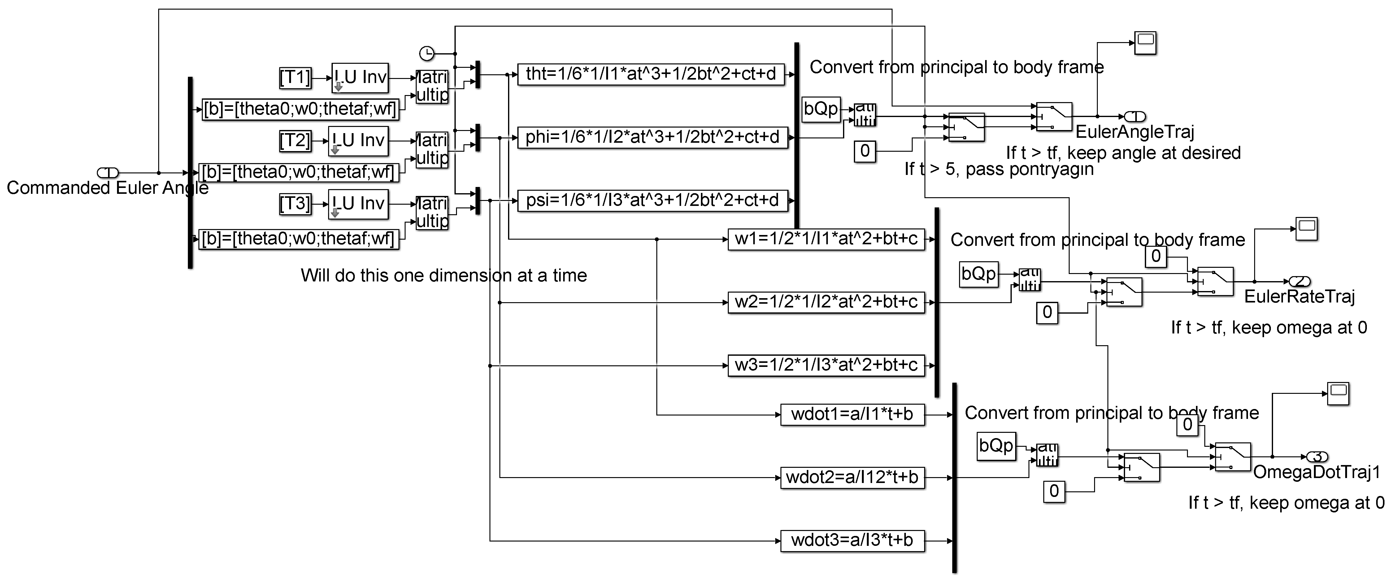
• Present and derive two methods of autonomous slew trajectory generation, sinusoidal and Pontryagin based generation.
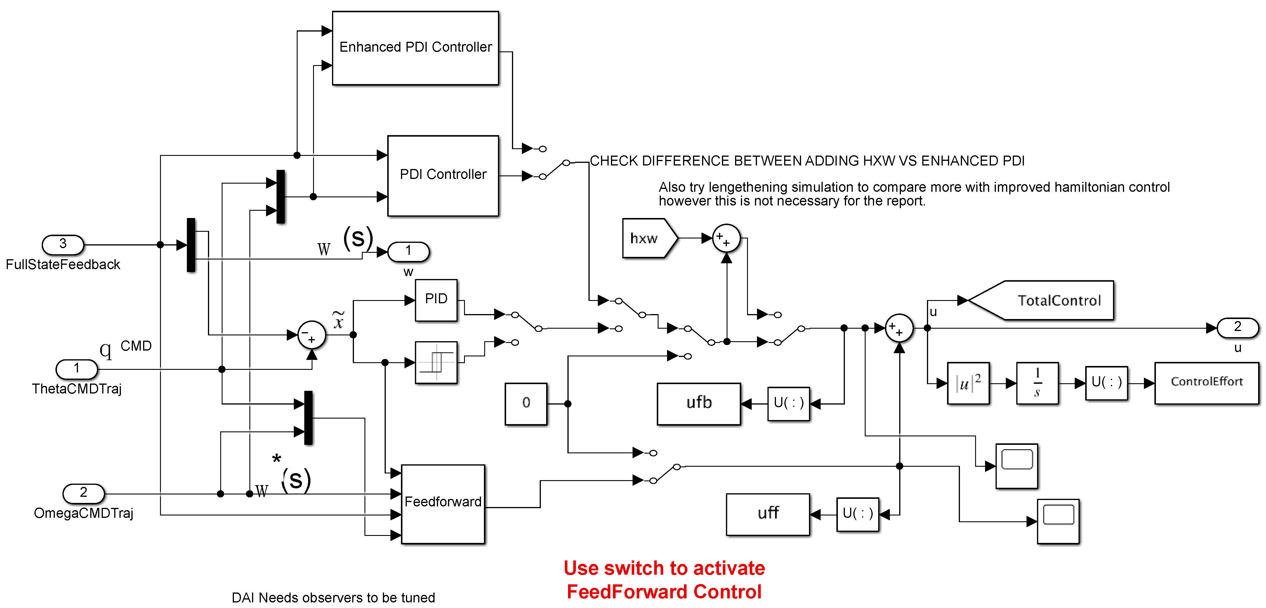
• Compare the performance of the derived trajectories when combined with various feedforward and feedback control schemes.
• Present two iterations on Pontryagin based trajectory generation and compare the instantiations.
• Validate the strength of trajectory-based control schemes over single-state feedback control methods.

The manuscript begins in Section 2 with a re-introduction of sinusoidal trajectory generation before deriving control minimizing (analytic) optimal trajectories using Pontryagin’s method of imposing necessary conditions of optimality followed by solution of boundary value problems for families of solutions. A brief presentation of each of the control methods follows. Section 3 presents the results of simulations of the control methods and lastly Section 4 discusses and interprets the results of Section 3.

2. Materials and Methods

2.1. Autonomous Trajectory Generation

Given an end state, the goal is for the system to autonomously generate a trajectory to follow. Two methods of doing so will be examined, trajectory generation by examining the structure of the problem and solution to efficient spacecraft slews, and trajectory generation using Pontryagin’s method, which consists of imposing necessary conditions of optimality to solve for the boundary values of the boundary value problems of optimal state rate and trajectory. The trajectory shall be composed of an initial quiescent period, followed by a slew, and ending in a final quiescent period.

2.1.1. Sinusoidal Trajectories

In response to a commanded slew, a spacecraft should quickly snap to the desired attitude, where the definition of quick is determined by the human controller. If attitude maneuvering were instantaneous, the plot of the spacecraft’s attitude representation would appear as a step function in the commanded maneuver channel. However, step functions are not smooth, represent discontinuities, and cannot be easily differentiated. Recognizing an instantaneous slew is impossible and a smooth, differentiable trajectory is optimal, we turn to an analysis of the structure of the problem.

Simple ordinary differential equations of the form $\dot{z}=Az$, such as a state space representation of spacecraft rotational dynamics, can be recognized as a harmonic oscillator, which has the solution of an exponential function of the form $z=A\exp \mathsf{\lambda }\mathrm{t},$ and can be written as a sinusoidal, $z=A\sin \left(\mathsf{\omega }\mathrm{t}\right)$ [6]. Given the structure of the solution to the dynamics, an idea is for the commanded slew to follow the sinusoidal structure. Studying the sine wave in Figure 2 demonstrates how a square wave can be approximated by a piecewise trajectory of an initial quiescent period, a sine wave with period approaching zero, and a final quiescent period. As sine waves are smooth and differentiable, sinusoidal structure readily lends itself to a sinusoidal trajectory generation scheme

A nominal sine curve is depicted above, note the abrupt start at time t = 0. A smooth initiation is preferable to avoid sudden impulsive maneuvers and undesirable resonance of flexible structures such as solar panels. In Figure 2b, at time $\mathrm{t}=\frac{3\mathrm{T}}{4}$, where $\mathrm{T}$ is the sine wave period, we note the smooth ramp up, indicating the derivative is zero and slowly increases rather than an initial derivative demanding immediate velocity. A non-instantaneous derivative reduces strain on the system. Thus time $\mathrm{t}=3\mathrm{T}/4$ is desirable for the slew start. Choosing the quiescent time, ${\Delta \mathrm{t}}_{\mathrm{quiescent}}$, the maneuver time, ${\Delta \mathrm{t}}_{\mathrm{maneuver}}$, the sinusoidal trajectory is designed in the following steps.

$$z=\sin \left(\mathsf{\omega }\mathrm{t}\right)$$

(1)

1.

The maneuver time, ${\Delta \mathrm{t}}_{\mathrm{maneuver}}$, determines the period of the sine wave. A sine wave takes half the period to go from the lowest value to the highest so the desired period should be twice the slew time. Thus,

$$\mathsf{\omega }=\frac{2\mathsf{\pi }}{\mathrm{T}}=\frac{2\mathsf{\pi }}{2{\Delta \mathrm{t}}_{\mathrm{maneuver}}}=\frac{\mathsf{\pi }}{{\Delta \mathrm{t}}_{\mathrm{maneuver}}}$$

(2)

2.

Phase shift the sine wave such that the desired low point at time $\mathrm{t}=\frac{3\mathrm{T}}{4}$, is at the desired maneuver start time after the initial ${\Delta \mathrm{t}}_{\mathrm{quiescent}}$, recalling a positive phase shift translates the sine wave in the negative direction and a negative phase shift translates the sine wave in the negative direction. We would like to translate the sine wave to the left by $\mathrm{t}=\frac{3\mathrm{T}}{4}$, resulting in the low point at time $\mathrm{t}=\frac{3\mathrm{T}}{4}$ instead occurring at time $\mathrm{t}=0$, and to the right by ${\Delta \mathrm{t}}_{\mathrm{quiescent}}$, shifting the low point to the start of the slew.

$$z=\sin \left(\mathsf{\omega }\left(\mathrm{t}+\mathsf{\varphi }\right)\right)$$

(3)

3.

Next, we would like to manipulate the amplitude of the sine wave to match the desired change in attitude.

$$\mathrm{A}=\left({\mathrm{A}}_{\mathrm{f}}-{\mathrm{A}}_0\right)$$

(4)

where ${\mathrm{A}}_{\mathrm{f}}$ is the final attitude desired, and ${\mathrm{A}}_0$ the initial attitude.

4.

Amplitude-shift the curve up for smooth initiation at ${\mathrm{A}}_0$ by adding ${\mathrm{A}}_0$.

$$z=\left({\mathrm{A}}_{\mathrm{f}}-{\mathrm{A}}_0\right)\left[1+\sin \left(\mathsf{\omega }\mathrm{t}+\frac{3{\Delta \mathrm{t}}_{\mathrm{maneuver}}}{2}-{\Delta \mathrm{t}}_{\mathrm{quiescent}}\right)\right]$$

(5)

5.

Craft a piecewise continuous trajectory with an initial quiescent period of ${\Delta \mathrm{t}}_{\mathrm{quiescent}}$, followed by the sinusoidal function formed in the preceding steps occurring during ${\Delta \mathrm{t}}_{\mathrm{maneuver}}$, and ending in a quiescent period of constant final attitude.

$$\mathrm{for}\{\begin{array}{c}\mathrm{t}<{\Delta \mathrm{t}}_{\mathrm{quiesant}}\\ {\Delta \mathrm{t}}_{\mathrm{quiescant}}\le \mathrm{t}<{\Delta \mathrm{t}}_{\mathrm{maneuver}}+{\Delta \mathrm{t}}_{\mathrm{quiescant}}\\ \mathrm{t}\ge {\Delta \mathrm{t}}_{\mathrm{maneuver}}+{\Delta \mathrm{t}}_{\mathrm{quiescant}}\end{array}\to \begin{array}{c}\mathrm{z}={\mathrm{A}}_0\\ \mathrm{z}=\left({\mathrm{A}}_{\mathrm{f}}-{\mathrm{A}}_0\right)\left[1+\sin \left(\mathsf{\omega }\mathrm{t}+\frac{3{\Delta \mathrm{t}}_{\mathrm{maneuver}}}{2}-{\Delta \mathrm{t}}_{\mathrm{quiescent}}\right)\right]\\ \mathrm{z}={\mathrm{A}}_{\mathrm{f}}\end{array}$$

(6)

Equation (6) can then be easily differentiated to solve for the state, rate, and acceleration.

2.1.2. Optimal Trajectory Using Pontryagin’s Method

Another technique of formulating the trajectory is by use of Pontryagin’s principle. Pontryagin’s principle forms a boundary value problem of the trajectory and makes use of necessary conditions of optimality to solve for the boundary values. The result is an optimal trajectory with respect to the cost function used.

Defining the Problem

The system consists of the 3 degree-of-freedom rotational motion of a rigid body, which when the angular velocity is measured in a non-inertial frame, is represented as

$$\underset{\begin{array}{c}\mathrm{External}\\ \mathrm{torque}\end{array}}{\underbrace{\mathrm{T}}}=\underset{\begin{array}{c}\mathrm{Double}\\ \mathrm{integrator}\end{array}}{\underbrace{\mathrm{I}\ddot{\mathsf{\theta }}}}+\underset{\begin{array}{c}\mathrm{Transport}\\ \mathrm{theorem}\end{array}}{\underbrace{\mathsf{\omega }\times \mathrm{I}}}$$

(7)

where $\mathrm{I}$ is the moment of inertia of the body, $\ddot{\mathsf{\theta }}$ is the second derivative of the state $\mathsf{\theta }$, which represents the three body angles, and $\mathrm{T}$ is the applied torque in the body frame. The initial states were initialized at zero, and the system was commanded to reach a final state of ${\mathsf{\theta }}_{\mathrm{d}}$, or a desired attitude, with a final angular velocity of zero, $\dot{\mathsf{\theta }}\left({\mathrm{t}}_{\mathrm{f}}\right)=0$. The model was built in Matlab Simulink and the block diagram can be found in Appendix A Figure A1.

The trajectory optimization problem begins with the dominant double-integrator dynamics as a quadratic control (DQC) problem, and can be summarized as Equation (8), whose result will yield optimal trajectories that are subsequently utilized to control the transport theorem terms.

$$\begin{array}{cc}\mathrm{Minimize}\hspace{1em}\hfill & \hfill \mathrm{J}\left[\mathrm{x}(\cdot ),\mathrm{u}(\cdot )\right]=1/2{{\displaystyle \int }}_{{\mathrm{t}}_0}^{{\mathrm{t}}_{\mathrm{f}}}{\mathsf{\tau }}^2\mathrm{dt}\end{array}$$

(8)

$$\begin{array}{cc}\mathrm{Subject\; to}\hspace{1em}\hfill & \dot{\mathsf{\theta }}=\mathsf{\omega }\\ & \dot{\mathsf{\omega }}=\mathsf{\tau }/\mathrm{I}\\ & \left({\mathsf{\theta }}_0,{\mathsf{\omega }}_0\right)=\left(0,0\right)\\ & \left({\mathsf{\theta }}_{\mathrm{f}},{\mathsf{\omega }}_{\mathrm{f}}\right)=\left(1,0\right)\\ & {\mathrm{t}}_0=0\\ & {\mathrm{t}}_{\mathrm{f}}=1\end{array}$$

The state is given by $\left[\mathsf{\theta },\mathsf{\omega }\right]$, the angle of rotation and angular velocity respectively. The value $\mathsf{\tau }$ is the control torque applied, and I, the inertia of the system, $\mathrm{J}$, the cost function, is the quadratic cost, computed by integrating the square of the applied torque. The quadratic cost represents the amount of work or energy needed to control the system and thus translates readily to quantities such as fuel used and real-world dollars. Note the simplification from Equation (7). In Equation (8), the acceleration should be $\dot{\mathsf{\omega }}=\mathsf{\tau }/\mathrm{I}-\mathsf{\omega }\times \mathrm{I}$, however, the cross-coupling makes the boundary value problem tricky to solve. Instead, the trajectory of each Euler angle can be solved for individually, under the assumption disregarding the cross-coupling effects does not affect optimality. To do so, the inertia matrix must also be manipulated, as the off-axis products of inertia complicates things as well. Three methods were used and compared, one where the principal axes and principal moments of inertia were found and the Euler trajectories found in the principal frame and then converted to the body frame, one where the principal moments of inertia were used but the trajectories not converted from principal to body frame, i.e., of the form ${\dot{\mathsf{\omega }}}_1={\mathsf{\tau }}_1/{\mathrm{I}}_1$, where the 1 subscript indicates the first Euler angle and the principal moment of inertia corresponding to the principal axis best aligned with the first body axis. Lastly, the off-axis products of inertia were simply ignored, and the body frame moments of inertia used in calculating the trajectories. These techniques result in independently solvable Euler angle trajectories.

Principles of Pontryagin: Optimal States, Rates, and Controls

Pontryagin’s principle consists of forming a boundary value problem by first forming a Hamiltonian function from the given cost function and dynamics, secondly minimizing the Hamiltonian with respect to the states, thirdly taking the derivative of the Hamiltonian with respect to the states to solve for the derivatives of the co-vectors of the states, and if needed, using the transversality of the endpoint Lagrangian to solve for the final values of the co-states and generate enough boundary conditions to solve the boundary value problem.

H: Form the Hamiltoninan

$$\mathrm{H}=\mathrm{F}+{\mathsf{\lambda }}^{\mathrm{T}}\mathrm{f}\left(\mathrm{x},\mathrm{u}\right)$$

(9)

where $\mathrm{F}$, is the running cost function, in general the part of the cost function being continuously integrated, in Equation (8), $1/2{\mathsf{\tau }}^2$, $\mathsf{\lambda }$ is the costate vector, given by $\left[{\mathsf{\lambda }}_{\mathsf{\theta }}{\mathsf{\lambda }}_{\mathsf{\omega }}\right]$, one costate per state, and $\mathrm{f}\left(\mathrm{x},\mathrm{u}\right)$ represents the dynamics of the system, $\dot{\mathrm{x}}$. In Equation (8) the state derivatives are $\mathrm{f}\left(\mathrm{x},\mathrm{u}\right)=\left[\begin{array}{cc}\mathsf{\omega }& \frac{\mathsf{\tau }}{\mathrm{I}}\end{array}\right]$.

$$\mathrm{H}=1/2{\mathsf{\tau }}^2+\left[{\mathsf{\lambda }}_{\mathsf{\theta }}{\mathsf{\lambda }}_{\mathsf{\omega }}\right]\left[\begin{array}{c}\mathsf{\omega }\\ \mathsf{\tau }/\mathrm{I}\end{array}\right]$$

(10)

Minimize the Hamiltonian

Pontryagin’s principle states the optimal solution can be found by taking the derivative of the Hamiltonian with respect to the control and setting the result equal to zero. Applying the derivative to Equation (10) and setting it equal to zero results in

$$\mathrm{dH}/\mathrm{du}=\mathrm{dH}/\mathrm{d}\mathsf{\tau }=\mathsf{\tau }+{\mathsf{\lambda }}_{\mathsf{\omega }}/\mathrm{I}=0$$

(11)

which gives $\mathsf{\tau }=-{\mathsf{\lambda }}_{\mathsf{\omega }}/\mathrm{I}$.

Adjoint Equation

The next step is to take the derivative of the Hamiltonian with respect to the states and set the result equal to the negative derivative of the co-states. Differentiating Equation (10) with respect to $\mathsf{\theta }$ and $\mathsf{\omega }$ results in

$$\mathrm{dH}/\mathrm{d}\mathsf{\theta }=-{\dot{\mathsf{\lambda }}}_{\mathsf{\theta }}=0\Rightarrow {\mathsf{\lambda }}_{\mathsf{\theta }}=\mathrm{a}$$

(12)

$$\mathrm{dH}/\mathrm{d}\mathsf{\omega }=-{\dot{\mathsf{\lambda }}}_{\mathsf{\omega }}=-{\mathsf{\lambda }}_{\mathsf{\theta }}\Rightarrow {\mathsf{\lambda }}_{\mathsf{\omega }}={\mathsf{\lambda }}_{\mathsf{\theta }}\mathrm{t}+\mathrm{b}=\mathrm{at}+\mathrm{b}$$

(13)

Terminal Transversality of the Endpoint Lagrangian

Conditions necessitating the use of terminal transversality of the endpoint Lagrangian are generally present when there are not enough boundary conditions to solve the boundary value problem formed in the previous steps. The method consists of forming a modified final cost function, $\overline{\mathrm{E}}$, from the final cost function, (in the problem of DQC, 0), plus the boundary conditions multiplied by unknown Lagrangians. The derivative of $\overline{\mathrm{E}}$, with respect to the endpoints ${\mathrm{x}}_{\mathrm{f}}$, equals the final values of the co-states. Luckily, for this problem terminal transversality is not required as the boundary value problem can already be solved.

The Boundary Value Problem

The boundary value problem can now be summarized as

$$\begin{array}{c}\dot{\mathsf{\theta }}=\mathsf{\omega }\\ \dot{\mathsf{\omega }}=\mathsf{\tau }/\mathrm{I}\\ \mathsf{\tau }=-\frac{{\mathsf{\lambda }}_{\mathsf{\omega }}}{\mathrm{I}}\\ {\mathsf{\lambda }}_{\mathsf{\theta }}=\mathrm{a}\\ {\mathsf{\lambda }}_{\mathsf{\omega }}=\mathrm{at}+\mathrm{b}\\ \left({\mathsf{\theta }}_0,{\mathsf{\omega }}_0\right)=\left(0,0\right)\\ \left({\mathsf{\theta }}_{\mathrm{f}},{\mathsf{\omega }}_{\mathrm{f}}\right)=\left(1,0\right)\\ {\mathrm{t}}_0=0\\ {\mathrm{t}}_{\mathrm{f}}=1\end{array}$$

(14)

Solving the problem gives an optimal solution for the state, rate, acceleration, and torque. Substituting the equation for ${\mathsf{\lambda }}_{\mathsf{\omega }}$ into the equation for the torque and integrating twice to find the optimal state and rate trajectories,

$$\begin{array}{c}\mathsf{\tau }=\left({\mathrm{I}}^{-1}\right)\left(-\mathrm{at}-\mathrm{b}\right)=\left({\mathrm{I}}^{-1}\right)\left(\mathrm{at}+\mathrm{b}\right)\\ \dot{\mathsf{\omega }}={\left({\mathrm{I}}^{-1}\right)}^2(1/2{\mathrm{at}}^2+\mathrm{bt}+\mathrm{c})\\ \mathsf{\theta }={\left({\mathrm{I}}^{-1}\right)}^2\left(1/6{\mathrm{at}}^3+1/2{\mathrm{bt}}^2+\mathrm{ct}+\mathrm{d}\right)\end{array}$$

(15)

Finally, the final values are used to solve for the coefficients and the solution for the optimal state, rate, and torque is as follows

$$\begin{array}{c}{\mathsf{\theta }}^{*}={\left({\mathrm{I}}^{-1}\right)}^2\left(3{\mathrm{t}}^2-2{\mathrm{t}}^3\right)\\ {\mathsf{\omega }}^{*}={\left({\mathrm{I}}^{-1}\right)}^2\left(6\mathrm{t}-6{\mathrm{t}}^2\right)\\ {\mathsf{\tau }}^{*}=\left({\mathrm{I}}^{-1}\right)\left(6-12\mathrm{t}\right)\end{array}$$

(16)

where * denotes the optimal solution. These optimal solutions to the trajectory are plotted in Figure 3 for a 30-degree yaw maneuver.

2.2. Feedback Controllers

A summary of the utilized controllers will be given in Section 2.2 beginning with Section 2.2.1, a standard proportional plus derivative (PD) controller establishing a classical performance benchmark, followed by a proportional plus integral plus derivative (PID) controller. A proportional plus derivative plus integral (PDI) control is introduced next in Section 2.2.3 followed by an enhanced PDI in Section 2.2.4. Feedforward controllers are introduced in Section 2.3 beginning with classical, ideal feedforward control in Section 2.3.1 followed by adaptive feedforward control in Section 2.3.2.

2.2.1. Proportional, Derivative (PD)

Given the desired final conditions are a function of the angle $\mathsf{\theta }$ and the angular velocity $\dot{\mathsf{\theta }}$, which is being driven to zero, a proportional derivative or PD controller is a logical choice. The PD controller computes the input to the plant, or the control as

$$\mathsf{\tau }={\mathrm{u}}_{\mathrm{fb}}=-{\mathrm{K}}_{\mathrm{d}}\left(\dot{\mathrm{q}}-{\dot{\mathrm{q}}}_{\mathrm{d}}\right)-{\mathrm{K}}_{\mathrm{p}}\left(\mathrm{q}-{\mathrm{q}}_{\mathrm{d}}\right)=-{\mathrm{K}}_{\mathrm{d}}\dot{\tilde{\mathrm{q}}}-{\mathrm{K}}_{\mathrm{p}}\tilde{\mathrm{q}}$$

(17)

where $\mathsf{\tau }$ is the control torque composed of the feedback control, ${\mathrm{K}}_{\mathrm{d}}$ and ${\mathrm{K}}_{\mathrm{p}}$ are the derivative and proportional gains respectively, $\mathrm{q}$ and $\dot{\mathrm{q}}$ are the state and state derivative, ${\mathrm{q}}_{\mathrm{d}}$ and $\dot{{\mathrm{q}}_{\mathrm{d}}}$ are the desired state and state derivative and the tilde represents the tracking errors, the error between the state and the desired state.

2.2.2. Proportional, Integral, Derivative (PID)

Another classical control choice is the proportional integral derivative controller. The PD controller computes the input to the plant, or the control as

$$\mathsf{\tau }={\mathrm{u}}_{\mathrm{fb}}=-{\mathrm{K}}_{\mathrm{p}}\left(\mathrm{q}-{\mathrm{q}}_{\mathrm{d}}\right)-{\mathrm{K}}_{\mathrm{d}}\frac{\mathrm{d}}{\mathrm{dt}}\left(\mathrm{q}-{\mathrm{q}}_{\mathrm{d}}\right)-{\mathrm{K}}_{\mathrm{I}}{\displaystyle \int }\left(\mathrm{q}-\mathrm{q}-\mathrm{d}\right)\mathrm{dt}$$

(18)

where $\mathsf{\tau }$ is the control torque, composed of the feedback control, ${\mathrm{K}}_{\mathrm{p}}$, ${\mathrm{K}}_{\mathrm{I}}$ and ${\mathrm{K}}_{\mathrm{d}}$, are the proportional, integral, and derivative gains respectively, $\mathrm{q}$ is the state, and ${\mathrm{q}}_{\mathrm{d}}$ $\dot{{\mathrm{q}}_{\mathrm{d}}}$ is the desired state.

2.2.3. Proportional, Derivative, Integral (PDI)

The proportional derivative integral controller differentiates itself from the PID controller by not differentiating the state to get the rate for calculation of the rate error. Instead, the PDI uses the rate from the state estimates directly. Eliminating the differentiation results in less noise in the error signal and smoother control. The PDI controller computes the input to the plant, or the control as displayed in Equation (19).

$$\mathsf{\tau }={\mathrm{u}}_{\mathrm{fb}}=-{\mathrm{K}}_{\mathrm{p}}\left(\mathrm{q}-{\mathrm{q}}_{\mathrm{d}}\right)-{\mathrm{K}}_{\mathrm{d}}\left(\dot{\mathrm{q}}-{\dot{\mathrm{q}}}_{\mathrm{d}}\right)-{\mathrm{K}}_{\mathrm{I}}{\displaystyle \int }\left(\mathrm{q}-{\mathrm{q}}_{\mathrm{d}}\right)\mathrm{dt}$$

(19)

2.2.4. Enhanced PDI

Given the non-linearities imposed by the transport theorem cross product in the system dynamics, a proposed improvement is the addition of a cross product term in the feedback control to account for the coupled motion [13]. The Enhanced PDI controller then has the form displayed in Equation (20)

$$\mathsf{\tau }={\mathrm{u}}_{\mathrm{fb}}=-{\mathrm{K}}_{\mathrm{p}}\left(\mathrm{q}-{\mathrm{q}}_{\mathrm{d}}\right)-{\mathrm{K}}_{\mathrm{d}}\left(\dot{\mathrm{q}}-{\dot{\mathrm{q}}}_{\mathrm{d}}\right)-{\mathrm{K}}_{\mathrm{I}}{\displaystyle \int }\left(\mathrm{q}-{\mathrm{q}}_{\mathrm{d}}\right)-\left(\dot{\mathrm{q}}-{\dot{\mathrm{q}}}_{\mathrm{d}}\right)\times \mathrm{I}\left(\dot{\mathrm{q}}-{\dot{\mathrm{q}}}_{\mathrm{d}}\right)$$

(20)

2.3. Feedforward Controllers

Feedback controllers are ubiquitously applicable to control systems from initial points to desired final points, utilizing a particular strength of feedback to imbue robustness. On the other hand, particularly when the goal is tracking a prescribed trajectory, tracking controllers are often of the feedforward nature lacking feedback, but instead emphasizing the analytic expressions of the controlled system dynamics and the prescribed desired trajectory. This section describes classical feedforward controllers first followed by nonlinear adaptive feedforward controllers (with a few disparate instantiations including various regression models and deterministic artificial intelligence).

2.3.1. Classical Feedforward Controller

Given the desired state, rate, and accelerations have been solved for, the feedforward control can be defined from an understanding of the system dynamics, and the feedforward control is displayed in Equation (21).

$$\mathsf{\tau }={\mathrm{u}}_{\mathrm{ff}}=\mathrm{I}{\dot{\mathsf{\omega }}}_{\mathrm{d}}+{\mathsf{\omega }}_{\mathrm{d}}\times \mathrm{I}{\mathsf{\omega }}_{\mathrm{d}}$$

(21)

Where the subscript refers to the desired trajectory. The control is formed by plugging in the desired states, rates, and accelerations, into equations of motion in Equation (7), giving us the control that should produce the desired states, rates, and accelerations, given perfect system modeling.

2.3.2. Adaptive Feedforward Development

If the dynamics were exactly always known, given a desired state trajectory, an ideal control could always be formulated and commanded, as in Equation (21), to accomplish the desired maneuver. However, in practicality, determining the inertia dyadic perfectly is very difficult, at best a close estimate is made, resulting in imperfect feedforward control. To better estimate the system and the ideal control, a method of updating the system model based off feedback error is proposed. For inertia matrix $\left[\mathrm{I}\right]$, Coriolis matrix $\left[\mathrm{C}\right]$, and applied external torque $\mathsf{\tau }$, the equations of motion are

$$\left\{{\mathsf{\tau }}_{\mathrm{ideal}}\right\}=\left[\mathrm{I}\right]\left\{\ddot{\mathrm{q}}\right\}+\left[\mathrm{C}\right]\left\{\dot{\mathrm{q}}\right\}=\left[\mathrm{I}\right]\left\{{\ddot{\mathrm{q}}}_{\mathrm{d}}\right\}+\left[\mathrm{C}\right]\left\{{\dot{\mathrm{q}}}_{\mathrm{d}}\right\}$$

(22)

where $\mathrm{q}$ is the state, and ${\mathrm{q}}_{\mathrm{d}}$ the desired state. In more common terms

$$\left\{{\mathsf{\tau }}_{\mathrm{ideal}}\right\}=\mathrm{I}\dot{\mathsf{\omega }}+\mathsf{\omega }\times \mathrm{I}\mathsf{\omega }=\left[\mathrm{I}\right]\left\{{\ddot{\mathrm{q}}}_{\mathrm{d}}\right\}+\left[\mathrm{C}\right]\left\{{\dot{\mathrm{q}}}_{\mathrm{d}}\right\}=\left[\mathsf{\Phi }\left({\mathsf{\omega }}_{\mathrm{d}},{\dot{\mathsf{\omega }}}_{\mathrm{d}}\right)\right]\left\{\mathsf{\theta }\right\}$$

(23)

The goal is to break the feedforward torque command into a regression model of a product of a matrix of knowns, $\left[\mathsf{\Phi }\right]$, times a vector of unknowns, $\left\{\mathsf{\theta }\right\}$. There are several choices available for the parameterization of $\left\{\mathsf{\theta }\right\}$, discussed in Section 2.3.3.

The adaptive aspect is an adaptation of the vector of unknowns, in response to error of the state with respect to the desired trajectory. The rate is defined in Equation (24).

$$\dot{\mathsf{\Theta }}=-{\mathsf{\Gamma }\mathsf{\Phi }}^{\mathrm{T}}\left(\dot{\tilde{\mathrm{q}}}+\mathsf{\lambda }\tilde{\mathrm{q}}\right)$$

(24)

where $\mathsf{\Gamma }>0$ and $\dot{\tilde{\mathrm{q}}}$ is the error in the state derivative with respect to the desired state derivative $\dot{\mathrm{q}}-{\dot{\mathrm{q}}}_{\mathrm{d}}$, as defined above. Equation (24) can be integrated starting from an initial estimate of $\mathsf{\Theta }$, to form a continuously learning, adaptive system.

Another choice is to form $\left[\mathsf{\Phi }\right]$ using reference trajectories is in Equation (25):

$${\dot{\mathrm{q}}}_{\mathrm{r}}={\dot{\mathrm{q}}}_{\mathrm{d}}-\mathsf{\lambda }\left(\mathrm{q}-{\mathrm{q}}_{\mathrm{d}}\right)={\dot{\mathrm{q}}}_{\mathrm{d}}-\mathsf{\lambda }\left(\tilde{\mathrm{q}}\right),{\ddot{\mathrm{q}}}_{\mathrm{r}}={\ddot{\mathrm{q}}}_{\mathrm{d}}-\mathsf{\lambda }\left(\dot{\mathrm{q}}-{\dot{\mathrm{q}}}_{\mathrm{d}}\right)={\ddot{\mathrm{q}}}_{\mathrm{d}}-\mathsf{\lambda }\left(\dot{\tilde{\mathrm{q}}}\right)$$

(25)

for $\mathsf{\lambda }>0$, at which point ${\mathrm{q}}_{\mathrm{d}}$ in Equation (23) would be replaced with ${\mathrm{q}}_{\mathrm{r}}$. Reference trajectories serve to compensate for the error in trajectory by giving a “boost”. For instance, if the state is lower than the desired state, to ensure the end conditions are still met, the state derivative should be slightly boosted, e.g., if the desired final state is five radians at time, t = 1, the desired state derivative a constant four radians per second, and rather than being at one radian, at time t=0 the state is at zero, then to arrive at the desired final state of five radians, the state derivative will need to be five radians per second assuming linear motion. The reference trajectory should in theory help ensure the final conditions are better met without the need for classical feedback control.

Through formulation of a Lyapunov function [4] and Barbarat’s lemma [6], control of the form of Equation (23) in conjunction with feedback control of the form of Equation (17), is proven stable, and the state error proven to tend to zero. The proof is omitted here for brevity but can be found in [6].

2.3.3. Regression Modeling

9-Parameter Regression

Parameter regression seeks to write the governing dynamics equations, Equations (2) and (3), as products of a matrix of knowns and a vector of unknowns. While the governing equations of motion are messy and nonlinear in the state, they are linear in terms of the inertia dyadic $\left[\mathrm{I}\right]$. Noting the state is already known for control purposes, and the inertia dyadic is the most difficult to estimate, Equation (3) can be separated into a matrix of knowns as a function of the state, and a vector of unknowns, a function of the inertia dyadic and the angular momentum $\mathrm{H}$. The presented 9-parameter regression model is derived in Slotine [4].

$${\left[\mathsf{\Phi }\left({\mathsf{\omega }}_{\mathrm{r}},{\dot{\mathsf{\omega }}}_{\mathrm{r}}\right)\right]}_{3\times 9}{\left\{\widehat{\mathsf{\Theta }}\right\}}_{9\times 1}=\left[\begin{array}{ccccccccc}{\dot{\mathsf{\omega }}}_{\mathrm{x}}& {\dot{\mathsf{\omega }}}_{\mathrm{y}}& {\dot{\mathsf{\omega }}}_{\mathrm{z}}& 0& 0& 0& 0& -{\mathsf{\omega }}_{\mathrm{z}}& {\mathsf{\omega }}_{\mathrm{y}}\\ 0& {\dot{\mathsf{\omega }}}_{\mathrm{x}}& 0& {\dot{\mathsf{\omega }}}_{\mathrm{y}}& {\dot{\mathsf{\omega }}}_{\mathrm{z}}& 0& {\mathsf{\omega }}_{\mathrm{z}}& 0& {\mathsf{\omega }}_{\mathrm{x}}\\ 0& 0& {\dot{\mathsf{\omega }}}_{\mathrm{x}}& 0& {\dot{\mathsf{\omega }}}_{\mathrm{y}}& {\dot{\mathsf{\omega }}}_{\mathrm{z}}& -{\mathsf{\omega }}_{\mathrm{y}}& {\mathsf{\omega }}_{\mathrm{x}}& 0\end{array}\right]\left\{\begin{array}{c}{\widehat{\mathrm{J}}}_{\mathrm{xx}}\\ {\widehat{\mathrm{J}}}_{\mathrm{xy}}\\ {\widehat{\mathrm{J}}}_{\mathrm{xz}}\\ {\widehat{\mathrm{J}}}_{\mathrm{yy}}\\ {\widehat{\mathrm{J}}}_{\mathrm{yz}}\\ {\widehat{\mathrm{J}}}_{\mathrm{zz}}\\ {\widehat{\mathrm{H}}}_{\mathrm{x}}\\ {\widehat{\mathrm{H}}}_{\mathrm{y}}\\ {\widehat{\mathrm{H}}}_{\mathrm{z}}\end{array}\right\}$$

(26)

Multiplying out the expression, Equation (26) is equivalent to Equation (3).

6-Parameter Regression

Recalling $\mathrm{H}=\mathrm{I}\mathsf{\omega }$, the nine-parameter model can be simplified to an equivalent six parameter model [6]:

$${\left[\mathsf{\Phi }\left({\mathsf{\omega }}_{\mathrm{r}},{\dot{\mathsf{\omega }}}_{\mathrm{r}}\right)\right]}_{3\times 6}{\left\{\widehat{\mathsf{\Theta }}\right\}}_{6\times 1}=\left[\begin{array}{cccccc}{\dot{\mathsf{\omega }}}_{\mathrm{x}}& {\dot{\mathsf{\omega }}}_{\mathrm{y}}& {\dot{\mathsf{\omega }}}_{\mathrm{z}}& -{\mathsf{\omega }}_{\mathrm{y}}{\mathsf{\omega }}_{\mathrm{z}}& 0& {\mathsf{\omega }}_{\mathrm{z}}{\mathsf{\omega }}_{\mathrm{y}}\\ {\mathsf{\omega }}_{\mathrm{x}}{\mathsf{\omega }}_{\mathrm{z}}& {\dot{\mathsf{\omega }}}_{\mathrm{x}}& 0& {\dot{\mathsf{\omega }}}_{\mathrm{y}}& {\dot{\mathsf{\omega }}}_{\mathrm{z}}& -{\mathsf{\omega }}_{\mathrm{z}}{\mathsf{\omega }}_{\mathrm{y}}\\ -{\mathsf{\omega }}_{\mathrm{x}}{\mathsf{\omega }}_{\mathrm{y}}& 0& {\dot{\mathsf{\omega }}}_{\mathrm{x}}& {\mathsf{\omega }}_{\mathrm{y}}{\mathsf{\omega }}_{\mathrm{x}}& {\dot{\mathsf{\omega }}}_{\mathrm{y}}& {\dot{\mathsf{\omega }}}_{\mathrm{z}}\end{array}\right]\left\{\begin{array}{c}{\widehat{\mathrm{J}}}_{\mathrm{xx}}\\ {\widehat{\mathrm{J}}}_{\mathrm{xy}}\\ {\widehat{\mathrm{J}}}_{\mathrm{xz}}\\ {\widehat{\mathrm{J}}}_{\mathrm{yy}}\\ {\widehat{\mathrm{J}}}_{\mathrm{yz}}\\ {\widehat{\mathrm{J}}}_{\mathrm{zz}}\end{array}\right\}$$

(27)

2.3.4. Deterministic Artificial Intelligence

Deterministic Artificial Intelligence begins with the same regression modeling as Adaptive Control, which can be portrayed as a statement of self, as the model is learning the system dynamics that govern itself. However, the crucial difference is the optimal learning of DAI. DAI uses the standard solution to the batch least squares regression problem [14,16]

$$\widehat{\mathsf{\theta }}={\left({\mathsf{\Phi }}^{\mathrm{T}}\mathsf{\Phi }\right)}^{-1}{\mathsf{\Phi }}^{\mathrm{T}}\mathrm{u}$$

(28)

where $\widehat{\mathsf{\Theta }}$ is estimated using feedback control, and the estimated states in $\mathsf{\Phi }$ are provided by a Luenberger Observer. Equation (28) represents optimal learning of the state. Differentiating Equation (28) results in Equation (29).

$$\mathsf{\delta }\widehat{\mathsf{\Theta }}={\left({\mathsf{\Phi }}^{\mathrm{T}}\mathsf{\Phi }\right)}^{-1}{\mathsf{\Phi }}^{\mathrm{T}}\mathsf{\delta }\mathrm{u}$$

(29)

which allows for the change in $\widehat{\mathsf{\Theta }}$ to be estimated and then integrated to get a smoother estimation of $\widehat{\mathsf{\Theta }}$. optimal learning expressed in Equations (28) and (29), with the declaration of self-awareness, learns the system parameters and can then be used to make an optimal feedforward control, ${\mathrm{u}}_{\mathrm{ff}}=\mathsf{\Phi }\widehat{\mathsf{\Theta }}$.

2.4. Luenberger Observer

A Luenberger Observer is used to estimate the control observed to act on the system. Given errors in the estimation of the inertia matrix, the control commanded will not result in the state and rate expected. Therefore, the Luenberger Observer examines the actual state and rate outputted by the plant and uses them to estimate the control responsible for the system response given the estimate of the inertia matrix, resulting in a simulated observer estimation of the control torque. The Luenberger Observer is of the form

$$\widehat{\mathsf{\theta }}={\displaystyle \int }\left[{\mathrm{J}}^{-1}{\displaystyle \int }\left({\mathrm{K}}_{\mathrm{p}}\mathrm{e}+{\mathrm{K}}_{\mathrm{i}}{\displaystyle \int }\mathrm{edt}\right)\mathrm{dt}+{\mathrm{K}}_{\mathrm{d}}\dot{\mathrm{e}}\right]\mathrm{dt}$$

(30)

where $\mathrm{e}$ is the error of the observed state. The torque can be extracted as

$$\mathsf{\tau }={\mathrm{K}}_{\mathrm{p}}\mathrm{e}+{\mathrm{K}}_{\mathrm{i}}{\displaystyle \int }\mathrm{e}\mathrm{dt}$$

(31)

And $\mathsf{\delta }\mathrm{u}$ in Equation (29) is found by subtracting the result of Equation (31) from the commanded torque outputted by the chosen controller.

2.5. Simulation

A simulation was developed in MATLAB Simulink to examine the difference between feedback control, adaptive feedforward control and feedback plus adaptive feedforward control. A timestep of 0.001 s was used in combination with a fourth-ordered Runge–Kutta integration solver.

3. Results

The various controllers and generation techniques were compared. For all controllers the gains were ${\mathrm{K}}_{\mathrm{P}}=\mathrm{100,000}$, ${\mathrm{K}}_{\mathrm{D}}=1000,{\mathrm{K}}_{\mathrm{I}}=10,\mathsf{\Gamma }=30,\mathsf{\lambda }=100$.

3.1. Comparison of Sinusoidal and Pontryagin Based Trajectory Generation

All the control methods presented in Section 2 were run, as well as all combinations of feedforward and feedback control techniques.

Table 1. System responses for various controller architectures in response to sinusoidal trajectory for a symmetric spacecraft.

Controller	Final Roll Error	Final Pitch Error	Final Yaw Error	Control Measure	Run Time
Classical Feedforward (FF)	$1.1611\times {10}^{-4}$	1.8036 $\times {10}^{-5}$	1.4804 $\times {10}^{-1}$	7.4211	10.6987
PID	1.7617$\times {10}^{-10}$	−1.7788 $\times {10}^{-11}$	5.3291 $\times {10}^{-14}$	7.7718	11.0032
PD	1.7617 $\times {10}^{-10}$	−1.7788 $\times {10}^{-11}$	5.3291 $\times {10}^{-14}$	7.5121	10.3543
PDI	1.7592 $\times {10}^{-10}$	−1.783 $\times {10}^{-11}$	−4.9919 $\times {10}^{-11}$	7.5121	11.5215
Enhanced PDI	1.7592 $\times {10}^{-10}$	−1.783 $\times {10}^{-11}$	−4.9919 $\times {10}^{-11}$	7.5121	10.9573
Adaptive Feedforward	1.18$\times {10}^{-10}$	1.8098 $\times {10}^{-5}$	−2.124 $\times {10}^{-2}$	7.3325	11.9128
DAI	1.1761 $\times {10}^{-10}$	1.8684 $\times {10}^{-5}$	1.4849 $\times {10}^{-1}$	7.4212	10.2718
Classical FF + PID	1.7617 $\times {10}^{-10}$	−1.7788 $\times {10}^{-11}$	5.3291 $\times {10}^{-14}$	7.7004	10.8363
Classical FF + PD	1.7617 $\times {10}^{-10}$	−1.7788 $\times {10}^{-11}$	5.3291 $\times {10}^{-14}$	7.452	10.6769
Classical FF + PDI	1.7592 $\times {10}^{-10}$	−1.783 $\times {10}^{-11}$	−3.2875 $\times {10}^{-10}$	7.452	10.7868
Classical FF + Enhanced PDI	1.7592 $\times {10}^{-10}$	−1.783 $\times {10}^{-11}$	−3.2875 $\times {10}^{-10}$	7.452	10.7328
Adaptive FF + PID	1.7617 $\times {10}^{-10}$	−1.7788 $\times {10}^{-11}$	5.3291 $\times {10}^{-14}$	7.7004	11.038
Adaptive FF + PD	1.7617 $\times {10}^{-10}$	−1.7788 $\times {10}^{-11}$	5.3291 $\times {10}^{-14}$	7.452	11.4322
Adaptive FF + PDI	1.7592 $\times {10}^{-10}$	−1.783 $\times {10}^{-11}$	−3.2954 $\times {10}^{-10}$	7.452	10.9991
Adaptive FF + Enhanced PDI	1.7592 $\times {10}^{-10}$	−1.783 $\times {10}^{-11}$	−3.2954 $\times {10}^{-10}$	7.452	10.9991
DAI + PID	1.7617 $\times {10}^{-10}$	−1.7788 $\times {10}^{-11}$	5.3291 $\times {10}^{-14}$	7.7004	12.2044
DAI + PD	1.7617 $\times {10}^{-10}$	−1.7788 $\times {10}^{-11}$	5.3291 $\times {10}^{-14}$	7.452	10.4896
DAI + PDI	1.7592 $\times {10}^{-10}$	−1.7829 $\times {10}^{-11}$	−3.2945 $\times {10}^{-10}$	7.452	11.211
DAI + Enhanced PDI	1.7592 $\times {10}^{-10}$	−1.7829 $\times {10}^{-11}$	−3.2945 $\times {10}^{-10}$	7.452	10.6421

shows the system responses when a sinusoidal trajectory was used, and

Table 2. System responses for various controller architectures in response to Pontryagin based trajectory for a symmetric spacecraft.

Controller	Final Roll Error	Final Pitch Error	Final Yaw Error	Control Measure	Run Time
Classical Feedforward (FF)	1.1611 $\times {10}^{-4}$	1.8452 $\times {10}^{-5}$	−1.8 $\times {10}^{-1}$	7.3137	10.7324
PID	1.7617 $\times {10}^{-10}$	−1.7788 $\times {10}^{-11}$	5.3291 $\times {10}^{-14}$	7.6889	10.6961
PD	1.7617 $\times {10}^{-10}$	−1.7788 $\times {10}^{-11}$	5.3291 $\times {10}^{-14}$	7.4272	10.7384
PDI	1.7592 $\times {10}^{-10}$	−1.783 $\times {10}^{-11}$	−4.9919 $\times {10}^{-11}$	7.4272	10.5332
Enhanced PDI	1.7592 $\times {10}^{-10}$	−1.783 $\times {10}^{-11}$	−4.9919 $\times {10}^{-11}$	7.4272	11.5323
Adaptive Feedforward	1.18 $\times {10}^{-4}$	1.8098 $\times {10}^{-5}$	−2.124 $\times {10}^{-2}$	7.3325	11.9128
DAI	1.1761 $\times {10}^{-4}$	1.8684 $\times {10}^{-5}$	1.4849 $\times {10}^{-1}$	7.4212	10.2718
Classical FF + PID	1.7617 $\times {10}^{-10}$	−1.7788 $\times {10}^{-11}$	5.3291 $\times {10}^{-14}$	7.6132	11.2188
Classical FF + PD	1.7617 $\times {10}^{-10}$	−1.7788 $\times {10}^{-11}$	5.3291 $\times {10}^{-14}$	7.3721	10.5145
Classical FF + PDI	1.7592 $\times {10}^{-10}$	−1.783 $\times {10}^{-11}$	−3.9984 $\times {10}^{-10}$	7.3721	11.6424
Classical FF + Enhanced PDI	1.7617 $\times {10}^{-10}$	−1.7788 $\times {10}^{-11}$	−3.9984 $\times {10}^{-10}$	7.3721	10.9332
Adaptive FF + PID	1.7617 $\times {10}^{-10}$	−1.7788 $\times {10}^{-11}$	5.3291 $\times {10}^{-14}$	7.6132	10.9133
Adaptive FF + PD	1.7617 $\times {10}^{-10}$	−1.7788 $\times {10}^{-11}$	5.3291 $\times {10}^{-14}$	7.3721	11.4322
Adaptive FF + PDI	1.7592 $\times {10}^{-10}$	−1.783 $\times {10}^{-11}$	−3.9918 $\times {10}^{-10}$	7.3721	11.1862
Adaptive FF + Enhanced PDI	1.7592 $\times {10}^{-10}$	−1.783 $\times {10}^{-11}$	−3.9918 $\times {10}^{-10}$	7.3721	10.8416
DAI + PID	1.7617 $\times {10}^{-10}$	−1.7788 $\times {10}^{-11}$	5.3291 $\times {10}^{-14}$	7.6132	11.821
DAI + PD	1.7617 $\times {10}^{-10}$	−1.7788 $\times {10}^{-11}$	5.3291 $\times {10}^{-14}$	7.3721	10.9259
DAI + PDI	1.7592 $\times {10}^{-10}$	−1.7829 $\times {10}^{-11}$	−3.9918 $\times {10}^{-10}$	7.3721	11.8363
DAI + Enhanced PDI	1.7592 $\times {10}^{-10}$	−1.7829 $\times {10}^{-11}$	−3.9918 $\times {10}^{-10}$	7.3721	10.5461

shows when Pontryagin’s method was used. For both tables a symmetric inertia matrix of [16.67 0 0; 0 16.67 0; 0 0 16.67], representing a small cube sat was used. Due to the symmetry, there were no complications due to cross-coupling.

3.2. Non-Symmetrical Inertia Matrix

The analysis in Section 3.1 was repeated with a non-symmetric inertia matrix of [90 10 10; 10 100 −20; 10 −20 250] with results displayed in

Table 3. System responses for various controller architectures in response to sinusoidal trajectory for a non-symmetric spacecraft.

Controller	Final Roll Error	Final Pitch Error	Final Yaw Error	Control Measure	Run Time
Classical Feedforward	−7.8465 $\times {10}^{-3}$	07.4289 $\times {10}^{-3}$	1.4755 $\times {10}^{-1}$	1683.1175	11.3062
PID	7.02999 $\times {10}^{-8}$	−1.4242 $\times {10}^{-3}$	3.2021 $\times {10}^{-7}$	1859.8548	11.0474
PD	4.6554 $\times {10}^{-8}$	4.2169 $\times {10}^{-3}$	−1.2343 $\times {10}^{-7}$	1856.8902	11.1187
PDI	1.2405 $\times {10}^{-7}$	8.0862 $\times {10}^{-8}$	−1.2423 $\times {10}^{-7}$	1856.8949	12.1823
Enhanced PDI	−7.7385 $\times {10}^{-5}$	−3.8538 $\times {10}^{-5}$	−1.2461 $\times {10}^{-7}$	1854.5367	10.8186
Adaptive Feedforward	−46.2241	12.0051	0.91503	1691.4834	11.3136
DAI	−23.5631	−6.9415	4.4973	1682.6394	11.4354
DAI + PID	5.2592 $\times {10}^{-8}$	2.7825 $\times {10}^{-8}$	−1.0617 $\times {10}^{-8}$	1683.4428	12.3925
DAI + PD	5.1693 $\times {10}^{-8}$	2.9962 $\times {10}^{-8}$	−2.7428 $\times {10}^{-8}$	1683.1285	11.1785
DAI + PDI	−1.2907 $\times {10}^{-7}$	6.8226 $\times {10}^{-8}$	−3.2272 $\times {10}^{-8}$	1683.1286	11.3506
DAI + Enhanced PDI	−7.738 $\times {10}^{-5}$	−3.8551 $\times {10}^{-5}$	−3.2648 $\times {10}^{-8}$	1680.7742	12.0274

. To eliminate the cross-coupling, the method of solving for the trajectory in the principal frame and then converting to the body frame was used.

3.3. Pontryagin Cross-Coupling Techniques

Noting the large spikes in cost in

Table 4. System responses for various controller architectures in response to Pontryagin derived trajectory for a non-symmetric spacecraft.

Controller	Final Roll Error	Final Pitch Error	Final Yaw Error	Control Measure	Run Time
Classical Feedforward	5.7025 $\times {10}^{-1}$	−3.9878	−4.671 $\times {10}^{-1}$	1685.6928	10.9308
PID	6.2024 $\times {10}^{-7}$	−1.3186 $\times {10}^{-6}$	1.0581 $\times {10}^{-5}$	6,039,807.0998	11.1978
PD	−1.4968 $\times {10}^{-7}$	5.0851 $\times {10}^{-7}$	−3.7909 $\times {10}^{-6}$	2,308,873.8017	10.7945
PDI	−7.6111 $\times {10}^{-7}$	4.6852 $\times {10}^{-6}$	−3.6072 $\times {10}^{-6}$	2,308,895.124	12.1382
Enhanced PDI	−7.6111 $\times {10}^{-7}$	4.6852 $\times {10}^{-6}$	−3.6072	2,308,895.125	10.7405
Adaptive Feedforward	−41.5959	7.5133	−1.8841	1661.3028	10.8365
DAI	−16.6137	−5.5011	1.1828	1576.6269	11.0189
DAI + PID	6.022 $\times {10}^{-7}$	−1.2758 $\times {10}^{-6}$	1.0244 $\times {10}^{-6}$	6,039,357.2503	12.3928
DAI + PD	−1.3938 $\times {10}^{-7}$	4.8404 $\times {10}^{-7}$	−3.5984 $\times {10}^{-6}$	2,307,705	10.6427
DAI + PDI	−7.5074 $\times {10}^{-7}$	4.6608 $\times {10}^{-6}$	−3.408 $\times {10}^{-6}$	2,307,726.8977	12.251
DAI + Enhanced PDI	−7.5074 $\times {10}^{-7}$	4.6608 $\times {10}^{-6}$	−3.408 $\times {10}^{-6}$	2,307,726.8977	11.9634

, the analysis of Table 4 was repeated, with Pontryagin trajectory solved by using the principal moments of inertia but not converting from the principal frame to the body and instead assuming the control could be taken to be the same in either frame. The results are in

Table 5. Controller analysis for Pontryagin generated trajectory without principal to body frame conversion.

Controller	Final Roll Error	Final Pitch Error	Final Yaw Error	Control Measure	Run Time
Classical Feedforward	1.94649 $\times {10}^{-2}$	1.6969 $\times {10}^{-2}$	−1.7869 $\times {10}^{-1}$	1658.712	11.9093
PID	7.3164 $\times {10}^{-8}$	−2.1048 $\times {10}^{-8}$	3.7374 $\times {10}^{-7}$	1914.5126	12.5761
PD	4.4187 $\times {10}^{-8}$	4.7793 $\times {10}^{-8}$	−1.6766 $\times {10}^{-7}$	1910.2443	11.9447
PDI	1.1956 $\times {10}^{-7}$	8.5436 $\times {10}^{-8}$	−1.6847 $\times {10}^{-7}$	1910.2511	11.6654
Enhanced PDI	−7.5271 $\times {10}^{-5}$	−3.7483 $\times {10}^{-5}$	−1.689 $\times {10}^{-7}$	1908.3834	13.7759
Adaptive Feedforward	−43.7245	11.2064	7.9855 $\times {10}^{-1}$	1667.4484	12.5086
DAI	−22.9724	−6.3489	3.938	1658.4612	12.3755
DAI + PID	5.4829 $\times {10}^{-8}$	2.2512 $\times {10}^{-8}$	3.1165 $\times {10}^{-8}$	1665.493	12.0513
DAI + PD	5.4538 $\times {10}^{-8}$	2.3202 $\times {10}^{-8}$	2.5734 $\times {10}^{-8}$	1665.1394	11.874
DAI + PDI	1.2938 $\times {10}^{-7}$	6.1282 $\times {10}^{-8}$	3.192 $\times {10}^{-8}$	1665.1394	11.6999
DAI + Enhanced PDI	−7.5261 $\times {10}^{-5}$	−3.7507 $\times {10}^{-5}$	3.1499 $\times {10}^{-8}$	1663.2691	12.6906

.

Lastly the three techniques for eliminating the cross-coupling in Pontryagin generation of optimal trajectories were compared for several different maneuvers. The maneuvers consisted of $\left[{\mathsf{\theta }}_{\mathrm{f}},{\mathsf{\varphi }}_{\mathrm{f}},{\mathsf{\psi }}_{\mathrm{f}}\right]$ where the final desired value for each maneuver was specified. Note ${\mathrm{K}}_{\mathrm{P}}$ and ${\mathrm{K}}_{\mathrm{D}}$ had to be raised to 100,000 and 10,000 respectively, to eliminate ringing in the second and third maneuvers. DAI + PD was used as the controller; the results are displayed in

Table 6. Comparison of various methods of cross-coupling elimination in Pontryagin trajectory generation versus sinusoidal trajectory generation for different maneuvers.

Trajectory Generation	Maneuver	Final Roll Error	Final Pitch Error	Final Yaw Error	Control Measure	Run Time
Sinusoidal	[0;0;30]	5.1819 $\times {10}^{-8}$	2.9662 $\times {10}^{-8}$	−2.5066 $\times {10}^{-8}$	1681.0949	11.687
Pontryagin in principal frame	[0;0;30]	−1.3882 $\times {10}^{-7}$	4.8269 $\times {10}^{-7}$	−3.5878 $\times {10}^{-6}$	2,304,236.6321	11.941
Pontryagin in non-principal frame with principal moments	[0;0;30]	5.4792 $\times {10}^{-8}$	2.26 $\times {10}^{-8}$	3.0474 $\times {10}^{-8}$	1662.3456	11.7472
Pontryagin in non-principal frame with non-principal moments	[0;0;30]	5.4792 $\times {10}^{-8}$	2.26 $\times {10}^{-8}$	3.0474 $\times {10}^{-8}$	1662.3456	12.62
Sinusoidal	[30;0;0]	1.9871 $\times {10}^{-8}$	3.1413 $\times {10}^{-9}$	−1.8097 $\times {10}^{-9}$	227.4904	11.4441
Pontryagin in principal frame	[30;0;0]	7.5466 $\times {10}^{-8}$	1.1922 $\times {10}^{-9}$	−6.9042 $\times {10}^{-10}$	5.1764 $\times {10}^9$	11.6651
Pontryagin non-principal frame with principal moments	[30;0;0]	1.9871 $\times {10}^{-8}$	3.1413 $\times {10}^{-9}$	−1.8097 $\times {10}^{-9}$	225.2765	11.6865
Pontryagin in non-principal frame with non-principal moments	[30;0;0]	1.9871 $\times {10}^{-8}$	3.1413 $\times {10}^{-9}$	−1.8097 $\times {10}^{-9}$	225.2765	11.952
Sinusoidal	[30;0;30]	1.9872 $\times {10}^{-8}$	3.1322 $\times {10}^{-9}$	−1.8096 $\times {10}^{-9}$	1921.2983	11.3724
Pontryagin in non-principal	[30;0;30]	1.2193 $\times {10}^{-8}$	1.9152 $\times {10}^{-9}$	−1.1148 $\times {10}^{-9}$	4.7500 $\times {10}^9$	11.4976
Pontryagin principal	[30;0;30]	1.9872 $\times {10}^{-9}$	3.1322 $\times {10}^{-9}$	−1.8096 $\times {10}^{-9}$	1896.2548	11.5732
Pontryagin in non-principal frame with non-principal moments	[30;0;30]	1.9872 $\times {10}^{-8}$	3.1322 $\times {10}^{-9}$	−1.8096 $\times {10}^{-9}$	1896.2548	11.4064

.

3.4. Constant Trajectory Feedback Control

For comparison, feedback control with a constant trajectory consisting of the desired end-state, was simulated. A PD controller was used with the same gains as in the previous simulations, ${\mathrm{K}}_{\mathrm{P}}=\mathrm{100,000}$, ${\mathrm{K}}_{\mathrm{D}}=1000$. The non-symmetric inertial-dyadic presented in Section 3.2 was used. The system response is given in Figure 4.

4. Discussion

Looking at Table 1 and Table 2, note the addition of feedforward decreases the control effort by 0.8% on average. Additionally, the three feedforward techniques seem to perform equally well. Comparing Table 2 with Table 1, Pontryagin trajectory generation lowers control cost by about 1–1.5%.

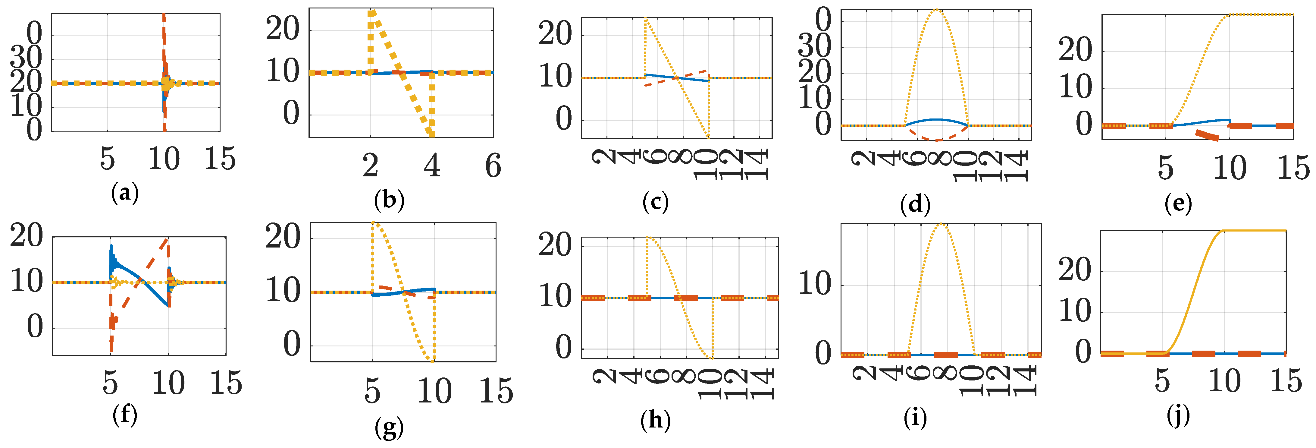
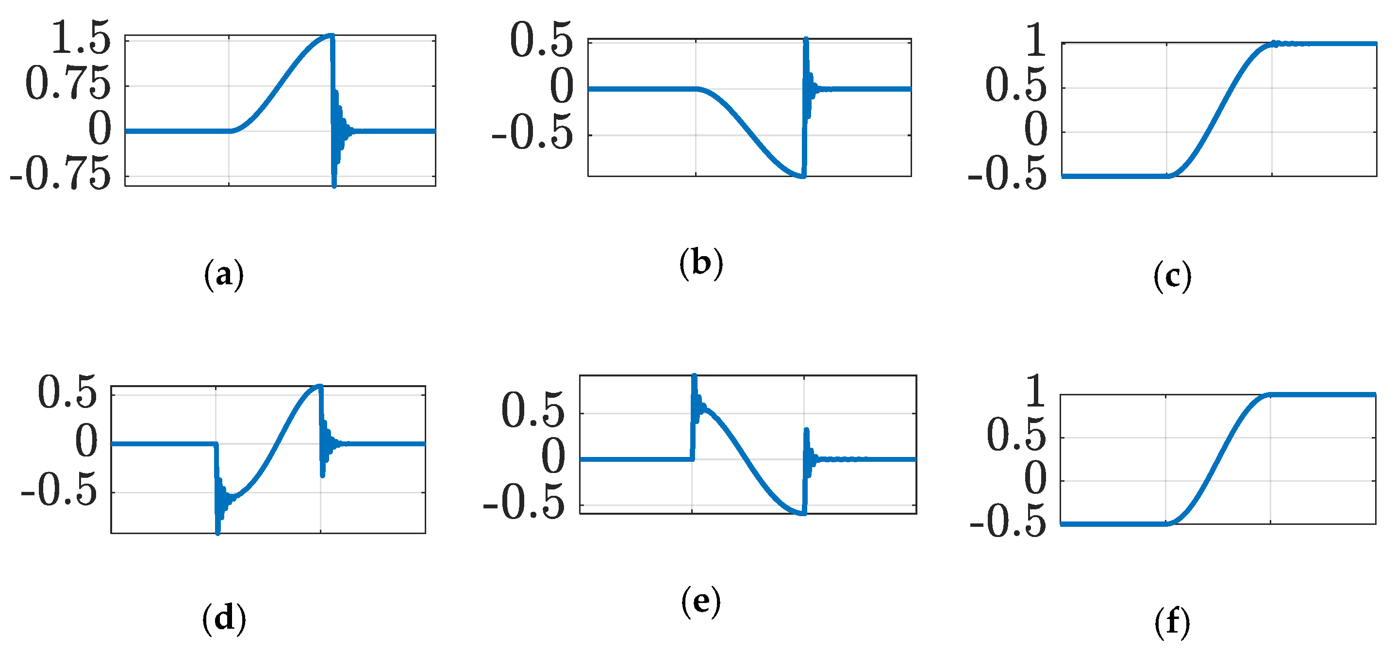
Looking at Table 3 and Table 4, Pontryagin techniques with feedback incur a lot of control cost. Examining the control torques and trajectories in Figure 5, reveals the Pontryagin method of converting from the principal frame to the body, commands motion in all three axes (see Figure 5e) due to the cross-coupling. Comparing Figure 5e with Figure 5f,d reveals the sinusoidal does not command motion in all three axes.

Looking at the tracking of the Euler angles in Figure 6, there is significant change in the non-slew directions. Once the slew is over, the error in commanding undesirable motion in the non-slew directions manifests itself in a spike of feedback control, making the control cost abnormally high. When Pontryagin is used without converting back into the body frame from the principal, essentially deriving a trajectory in the non-principal frame, undesirable motion in the non-slew directions was eliminated. In the formulation used in Figure 6 and by virtue of non-zero cross-products of inertia, principal axes were mis-aligned with the body axes, and while a seemingly fine idea, solving for the trajectory in the principal frame and then converting to the body frame introduces error. The misalignment causes undesired rotation in the body frame when the trajectory is converted, via cross-coupled terms in the inertia dyadic.

Table 5 proves not converting between principal and body frames fixes the error. Table 5 also demonstrates the flexibility of the control architecture, with low error independent of which axis was being rotated around. The disparity between principal moments of inertia and moments of inertia in the body frame, 81.5970, 105.326, 253.0783, compared with 90, 100, 250, is worth noting. Using the moments of inertia in the body frame to solve for the optimal trajectory in Pontryagin’s method applied in the non-principal frame, was predicted to have a detrimental effect, as the control might not be scaled properly. However, Table 6 shows no difference between using principal or non-principal moments of inertia.

Figure 4 shows the stark contrast between using a calculated trajectory and not. Comparing Figure 4b to the PD control in Table 5, note similar final errors in roll pitch and yaw channels, and five orders of magnitude worse control cost. In

Table 7. Comparison of PD control with and without Pontryagin Optimal Trajectory in non-principal frame with elevated gains of ${\mathrm{K}}_{\mathrm{P}}=\mathrm{1,000,000}$ and ${\mathrm{K}}_{\mathrm{D}}=\mathrm{10,000}$.

Controller	Final Roll Error	Final Pitch Error	Final Yaw Error	Control Measure	Run Time
PD w/Trajectory	5.3161 $\times {10}^{-9}$	2.6474 $\times {10}^{-9}$	3.5527 $\times {10}^{-15}$	1687.5	9.0155
PD w/o Trajectory	2.8341 $\times {10}^{-8}$	1.416 $\times {10}^{-8}$	3.5527 $\times {10}^{-15}$	3.4862$\times {10}^9$	8.648

, the PD controller gains were raised revealing that use of a calculated trajectory results in better final state error as compared to control without a calculated trajectory. Additionally, in response to elevated gains, control cost rose by a factor of ten in the non-trajectory case (between Figure 4b and the second row of Table 7), however when using Pontryagin optimal trajectory, the control cost actually decreased in response to elevated gains, by 11.7% (comparing the third row of Table 5 and the first row of Table 7) while the error decreased by an order of magnitude in the roll and pitch channels, and seven orders of magnitude in the yaw channel. The use of a calculated trajectory is thus shown to allow for higher gains that result in significantly lower error, and lower control cost. Additionally, the plotted system response with no calculated trajectory in Figure 4a, shows significant overshoot and significant oscillatory motion as compared to using a calculated trajectory.

As for a computational burden analysis, run time was recorded in each of the trials. Unfortunately, run-time was found to be dependent on the hardware the simulation was run on and how much of the CPU was available, resulting in an inability to compare run time across different tables. However, looking at each table individually, no run time different of more than 20% was observed, and no observable patterns found. With more detailed analysis it could be concluded whether any of the control methods used were more computationally demanding than the others, however for the purpose of this study, all control methods were deemed relatively similar in terms of computational burden.

4.1. Conclusions

Trajectory generation demonstrates significant decrease in control cost and attitude error as well as allowing for more versatile gain tuning. Pontryagin’s method shows promise, lowering control cost slightly over Sinusoidal generation and lays the groundwork for more sophisticated autonomous trajectory generation, by modification of the Hamiltonian (Equations (9) and (10)), such as imposition of pointing restraints, not possible with the sinusoidal method. Proper understanding of cross-coupling dynamical effects proved crucial in the formulation of Pontryagin’s method, however proving simple to deal with. Lower pointing errors make missions focused on objects further away, or requiring higher magnification and object resolution, possible, and lower control costs improve the efficiency of such missions, increasing viability.

4.2. Future Work

RTOC was not implemented and studied. RTOC inherently uses the trajectory solved for in Pontryagin’s method and a comparison of RTOC to control using sinusoidal trajectory generation would be interesting. Additionally, the assumption to solve for each Euler angle trajectory separately using Pontryagin’s method, inherently introduces some error. The amount of error in this formulation should be examined. A better approach would be to solve Pontryagin’s method for the full coupled dynamics. While there do exist methods to do so, they lie outside of the scope of this work were not attempted.

Of note, results are possible with higher gains and modest increases in cost. However, the investigation of this work was not into achieving the lowest error possible.

The true power of Pontryagin’s method lies in the ability to parameterize desired trajectories and solve for optimal solutions. For instance, during a slew a requirement might be specified declaring the spacecraft shall never point in a certain direction. With sinusoidal trajectory generation, there is no way to enforce a requirement on pointing restrictions without analysis of the sinusoidal trajectory and careful design of piecewise maneuvers around restrictions. However, Pontryagin’s method allows for such specifications in the formation of the Hamiltonian. Pontryagin’s method could significantly reduce control efforts of more complicated maneuvers with pointing restriction.

References

1. NASA to Provide Update on James Webb Space Telescope. 15 July 2020 MEDIA ADVISORY M20-083. Available online: https://www.nasa.gov/press-release/nasa-to-provide-update-on-james-webb-space-telescope (accessed on 2 March 2020).
2. NASA Image Use Policy. Available online: https://gpm.nasa.gov/image-use-policy (accessed on 23 December 2021).
3. Garner, R. Landsat Overview. NASA. Available online: https://www.nasa.gov/mission_pages/landsat/overview/index.html (accessed on 1 April 2015).
4. Slotine, J.-J.E.; Weiping, L. Applied Nonlinear Control; Prentice-Hall: Hoboken, NJ, USA, 1991. [Google Scholar]
5. Fossen, T. Comments on Hamiltonian adaptive control of spacecraft by Slotine, J.J.E. and Di Benedetto, M.D. IEEE Trans. Autom. Control. 1993, 38, 671–672. [Google Scholar] [CrossRef]
6. Sands, T.; Kim, J.; Agrawal, B. Improved Hamiltonian Adaptive Control of spacecraft. In Proceedings of the IEEE Aerospace Conference, Big Sky, MT, USA, 11 May 2009. [Google Scholar] [CrossRef]
7. Sands, T.; Kim, J.; Agrawal, B. Spacecraft Adaptive Control Evaluation. In Proceedings of the Infotech@Aerospace 2012, Garden Grove, CA, USA, 19–21 June 2012. [Google Scholar] [CrossRef]
8. Garcia, I.; How, J. Trajectory Optimization for Satellite Reconfiguration Maneuvers with Position and Attitude Constraints. In Proceedings of the American Control Conference, Portland, OR, USA, 8–10 June 2005. [Google Scholar] [CrossRef] [Green Version]
9. Sanyal, A.; Fosbury, A.; Chaturvedi, N.; Bernstein, D. Inertia-free Spacecraft Attitude Trajectory Tracking with Internal-Model-Based Disturbance Rejection and Almost Global Stabilization. In Proceedings of the American Control Conference, St. Louis, MO, USA, 10–12 June 2009. [Google Scholar]
10. Yoshimura, Y.; Matsuno, T.; Hokamoto, S. Global trajectory design for position and attitude control of an underactuated satellite. Trans. Jap. Soc. Aero. Space Sci. 2016, 59, 107–114. [Google Scholar] [CrossRef] [Green Version]
11. Zhang, L.; Yu, C.; Zhang, S.; Cai, H. Optimal attitude trajectory planning method for CMG actuated spacecraft. Proc. Inst. Mech. Eng. Part G J. Aero. Eng. 2018, 232, 131–142. [Google Scholar] [CrossRef]
12. Li, X.; Warier, R.R.; Sanyal, A.K.; Qiao, D. Trajectory tracking near small bodies using only attitude control. J. Guid. Control. Dyn. 2019, 42, 109–122. [Google Scholar] [CrossRef]
13. Baker, K.; Cooper, M.; Heidlauf, P.; Sands, T. Autonomous Trajectory Generation for Deterministic Artificial Intelligence. Electr. Electron. Eng. 2018, 8, 59–68. [Google Scholar] [CrossRef]
14. Sands, T. Development of Deterministic Artificial Intelligence for Unmanned Underwater Vehicles (UUV); MDPI, Multidisciplinary Digital Publishing Institute: Basel, Switzerland, 2020; Available online: https://www.mdpi.com/2077-1312/8/8/578/htm (accessed on 23 December 2021).
15. Walker, A. Genetic Fuzzy Attitude State Trajectory Optimization for a 3U Cube Sat. Ph.D. Dissertation, University of Cincinnati, Cincinnati, OH, USA, 15 June 2020. [Google Scholar] [CrossRef]
16. Smeresky, B.; Rizzo, A.; Sands, T. Optimal Learning and Self-Awareness Versus PDI. Algorithms 2020, 13, 23. [Google Scholar] [CrossRef] [Green Version]
17. Chen, C.; Guo, W.; Wang, P.; Sun, L.; Zha, F.; Shi, J.; Li, M. Attitude Trajectory Optimization to Ensure Balance Hexapod Locomotion. Sensors 2020, 20, 6295. [Google Scholar] [CrossRef] [PubMed]
18. Zhou, Q.; Liu, X.; Cai, G. Base attitude disturbance minimizing trajectory planning for a dual-arm space robot. Proc. Inst. Mech. Eng. Part G J. Aero. Eng. 2021. [Google Scholar] [CrossRef]
19. Malyuta, D.; Reynolds, T.; Szmuk, M.; Lew, T.; Bonalli, R.; Pavone, M.; Acikmese, B. Convex Optimization for Trajectory Generation. arXiv 2021, arXiv:2106.09125. [Google Scholar]
20. Sin, E.; Arcak, M.; Nag, S.; Ravindra, V.; Li, L.; Levinson, R. Attitude Trajectory Optimization for Agile Satellites in Autonomous Remote Sensing Constellations. In Proceedings of the AIAA Scitech Forum, Virtual Online Event, 4 January 2021. [Google Scholar] [CrossRef]
21. Sanyal, A.; Fosbury, A.; Chaturvedi, N.; Bernstein, D. Inertia-Free Spacecraft Attitude Tracking with Disturbance Rejection and Almost Global Stabilization. In Proceedings of the American Control Conference, Hyatt Regency Riverfront, St. Louis, MO, USA, 10–12 June 2009. [Google Scholar] [CrossRef] [Green Version]
22. Walker, A.; Putman, P.; Cohen, K. Solely Magnetic Genetic/Fuzzy-Attitude-Control Algorithm for a CubeSat. J. Space. Rock. 2015, 52, 1627–1639. [Google Scholar] [CrossRef]
23. Sands, T. Virtual Sensoring of Motion Using Pontryagin’s Treatment of Hamiltonian Systems. Sensors 2021, 21, 4603. [Google Scholar] [CrossRef] [PubMed]
Figure 1. James Webb telescope positions in the second Lagrange point, L2 from which attitude maneuvers point the telescope towards distant targets in outer space. [1] Image used consistent with NASA policy, “NASA content (images, videos, audio, etc.) are generally not copyrighted and may be used for educational or informational purposes without needing explicit permissions” [2].
Aerospace 09 00135 g001
Figure 2. (a) Piecewise sinusoidal trajectory with a slew time/maneuver time of 5 s and a quiescent time of 5 s before and after the slew (b) A nominal sine wave used to reveal relationship between points on the curve’s time and phase angle.
Aerospace 09 00135 g002
Figure 3. Optimal Trajectories from Pontryagin’s Method with time in seconds on the abscissas. (a) angular acceleration ω ˙ ( t ) on the ordinate, (b) angular velocity ω ( t ) on the ordinate, (c) angular displacement θ ( t ) on the ordinate. Note the similarity in the (c) to Figure 2a.
Aerospace 09 00135 g003
Figure 4. System response of PD control with constant trajectory. (a) Plot of Euler angles during the maneuver. Roll is solid blue, pitch is thick dashed red, yaw is thin dashed yellow (b) Characteristics of the response. * Note, this run time was found to be much lower due to differences in available processing power and when compared to re-simulations of some of the above methods, found to be comparable.
Aerospace 09 00135 g004
Figure 5. Comparison of system response to Pontryagin generated trajectory and Sinusoidal trajectory. Roll angle in degrees is displayed as a solid, blue line; pitch angle as a dashed red line, and yaw angle as a dotted gold line. The top row displays results using Pontryagin, while the bottom row displays results using Sinusoidal. (a) Feedback Control Pontryagin, (b) Feedforward Control Pontryagin, (c) Acceleration Trajectory Pontryagin, (d) Rate Trajectory Pontryagin, (e) State Trajectory Pontryagin, (f) Feedback Control Sinusoidal, (g) Feedforward Control Sinusoidal, (h) Acceleration Trajectory Sinusoidal, (i) Rate Trajectory Sinusoidal, (j) State Trajectory Sinusoidal.
Aerospace 09 00135 g005
Figure 6. Comparison of True Euler angles during slew, (a,d) roll, (b,e) pitch, and (c,f) yaw. Top row (ac) using Pontryagin derivation in principal frame, bottom row (df) using Pontryagin derivation in non-principal frame. (a) roll using principal frame, y-axis [−1,1.5] (b) pitch in principal frame, y-axis [−4,2], (c) yaw using principal frame, y-axis [0,30], (d) roll using non-principal, y-axis [−1.5 × 10−3,1 × 10−3], (e) pitch using non-principal axis, y-axis [−3 × 10⁻³, 4 × 10⁻³], (f) yaw using non-principal, y-axis [0,30].
Aerospace 09 00135 g006