Reliability-Oriented Configuration Optimization of More Electrical Control Systems

Abstract

More electrical vehicles adopt dissimilar redundant control systems with dissimilar power supplies and dissimilar actuators to achieve high reliability and safety, but this introduces more intricacy into the configuration design. Currently, it is difficult to identify the optimum configuration via the conventional trial-and-error approach within an acceptable timeframe. Hence, it is imperative to discover novel methods for the configuration design of more electrical vehicles. This paper introduced the design specification of more electric vehicles and investigated the contribution of different kinds of actuators, presenting a new multi-objective configuration optimization approach on the foundation of system reliability, weight, power, and cost. By adopting the non-dominated sorting genetic algorithm-II (NSGA-II), the Pareto optimization design set was obtained. Then, the analytic hierarchy process (AHP) was introduced to make a comprehensive decision on the schemes in the Pareto set and determine the optimal system configuration. Eventually, numerical results indicated that the reliability of our designed configuration increased by 5.89% and 55.34%, respectively, compared with dual redundancies and single redundancy configurations, which verified the effectiveness and practicability of the proposed method.

1. Introduction

Safety critical systems in aircraft [1], carrier rockets [2], ships [3] and large machines [4] usually adopt redundant actuation systems to guarantee high reliability and safety [5]. In such designs, the rest systems can complete the work when one or more actuators fail. To reduce the number of common-cause faults and common-mode faults, dissimilar redundancy systems are adopted consequentially [6], in which different actuators with the same performances are used. With the rapid development of more electrical technologies, and more electric vehicles based on different power supply systems, actuation systems and computers have become increasingly common. In terms of actuation systems, hydraulic actuators (HAs), electro-hydrostatic actuators (EHAs) and electromechanical actuators (EMAs) [7] are leveraged in more electric vehicles. For instance, more electrical aircrafts are adopting heterogeneous actuation systems to move control surfaces based on HAs and EHAs [8]. Since HAs utilize hydraulic power supply systems while EHAs and EMAs adopt electrical power supply systems, the configuration design of more electric vehicles (MEVs) faces substantial challenges. The first one is how to design more electric control systems to maintain high mission reliability without permissive cost and weight. The second one is how to strike a balance between power supply systems and actuator distribution. The last one is how to determine the types of actuators for more electric control systems, which include HAs, EHAs, and EMAs. Given the aforementioned factors, the design of safety-critical system configurations becomes a daunting task. Therefore, an appropriate and effective approach should be adopted to solve the combination-explosion problem of system configurations, thus achieving the optimization design of a more electric control system (MECS) [9,10].

The optimization design of an electric control system needs to realize multi-objective optimization and comprehensively consider various contradictory indicators. Traditional methods include the weighting method [11,12], the constraint method [13,14], and goal programming [15,16,17]. However, these methods require the designer to master corresponding background knowledge to determine weights, energy dissipation, and other indicators, and the explosive configuration is another challenge that arises from those methods. In addition, the program needs to be run independently many times, which may lead to inconsistent results each time and render it more difficult for designers to make eventual decisions. In recent decades, various multi-objective intelligent optimization algorithms have emerged and vigorously developed, for example, the genetic algorithm (GA) [18], differential evolution algorithm (DE) [19], particle swarm optimization algorithm (PSO) [20,21], and non-dominated sorting genetic algorithm (NSGA) [22]. Among them, NSGA is famous for its good performance due to the adoption of non-dominated sorting and fitness-sharing strategy. The former increases the possibility of superior characteristics inherited by the next generation, while the latter sustains population diversity, overcoming the overmuch reproduction of super individuals and preventing prematurity convergence [23]. Nevertheless, there are also disadvantages such as high computational complexity in NSGA. Thus, in 2002, Deb et al. proposed NSGA-II [24]. In contrast to NSGA, the rapid non-dominated sorting method, elitism preservation strategy and congestion comparison were introduced in NSGA-II, which greatly reduced the computational complexity of the algorithm. Moreover, NSGA-II also expanded the distribution space of the solution set in the Pareto frontier, thus maintaining population diversity [25]. At present, NSGA-II has been widely applied to tackle multi-objective optimization problems in various fields. Xia et al. [26] investigated the multi-objective optimization problem for AUV conceptual design, where NSGA-II was applied to find the optimal Pareto frontier, with a comprehensive consideration of cost, effectiveness, and risks. The result verified the effectiveness of the algorithm. Alam et al. [27] studied the problem of AUV design and construction and employed NSGA-II to determine the optimum design of a torpedo-like AUV with a total length of 1.3 m. In addition, a kind of heavier-than-water underwater vehicle (HUV) was regarded as a research object by Liu et al. [28], and NSGA-II was adopted to establish a global approximation model, thus assisting the eventual optimal design of HUV. Nevertheless, these methods ignored the optimization designs of the global architectures of dissimilar control systems. As mentioned above, the optimization design of MECS is to solve the multi-objective optimization issue, where some contradictory indicators require all-round considerations. Therefore, the NSGA-II, combined with the AHP [29,30,31,32] method, was adopted in this paper to solve this problem, in which the binary encoding mode was employed and the decision variables were confined in discrete space. Moreover, the mutation process was modified to better match the characteristics of the problem. Eventually, the case study verified the validity of our approach.

The other sections of the paper are arranged as follows: Section 2 demonstrates the system descriptions. Section 3 presents the optimization approach on the foundation of NSGA-II and AHP method. Section 4 displays the case study, while the conclusions are presented in Section 5.

2. Mathematical Modeling of More Electric Control System (MECS)

According to the design specification of safety critical systems, more electric control systems require high reliability and safety. For example, the possibility of mission failure per flight owing to certain material damages in the flight control system should not surpass the upper limit. Normally, the failure rate of a flight control system is ${10}^{-9}/h$ to ${10}^{-10}/h$ for a commercial aircraft. Hence, it is necessary to utilize a dissimilar flight control system to maintain high reliability.

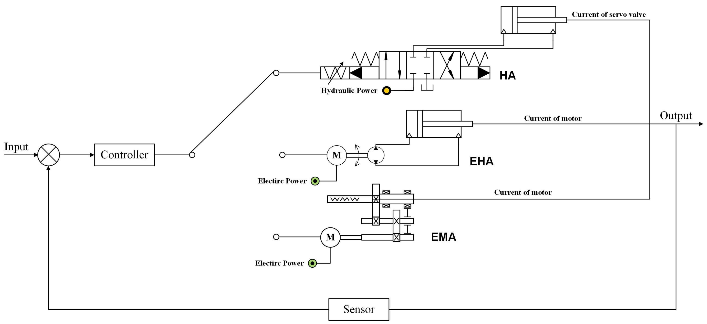
2.1. Single Control System Structure

A schematic diagram of the basic structure of a more electric control system, in which the controller, actuator, and sensor are main components, is illustrated in Figure 1. Since the electric power supply and hydraulic power supply are provided simultaneously, the actuator can be selected from HAs, EHAs, or EMAs, as shown in Figure 1. A HA is powered by a hydraulic supply system while an EHA or EMA is powered by an electric supply system. Since a centralized hydraulic power supply system has the characteristics of high-power density and fast response, HAs are widely used in control systems. However, the control system is heavy and easily exposed to oil contamination when HAs are adopted as they need pipeline transmission from the centralized power supply to the actuator. An EHA consists of the motor, pump, and cylinder that replaces the pipeline transmission by wire transmission. Hence, the weight of an EHA is light, whereas its heat dissipation is poor. An EMA consists of the motor and the ball screws. The command is transmitted from the wire controlling the motor and ball screws to drive the load. Therefore, an EMA is simple and light weight, but it gets stuck easy. Hence, to determine which type of actuator should be used, one has to comprehensively consider the weight, performance, and reliability.

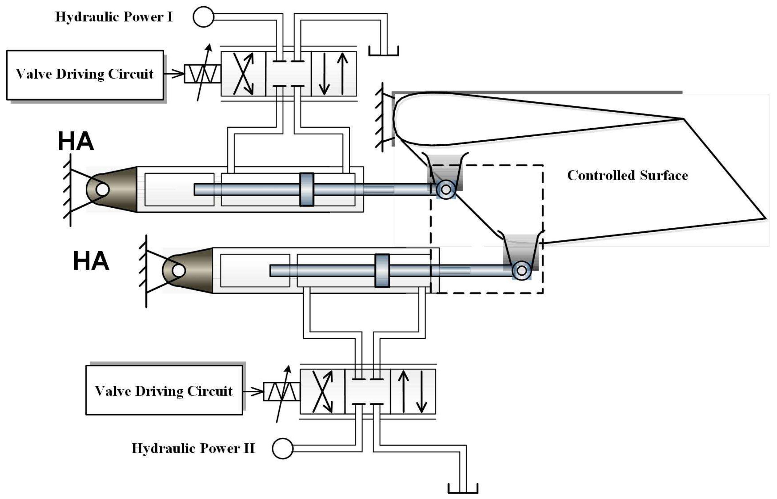
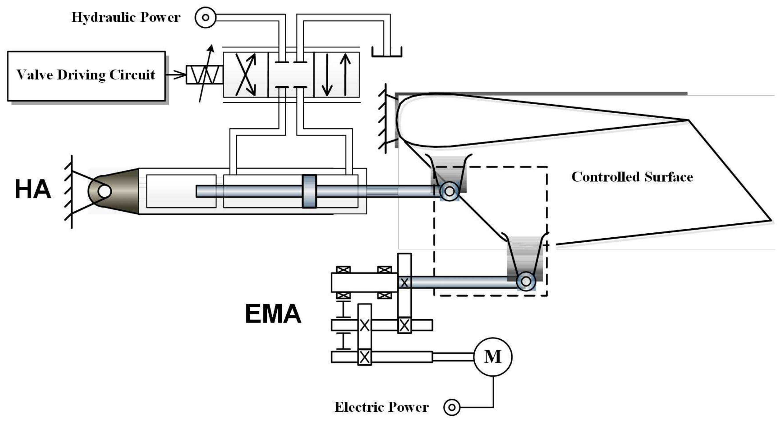
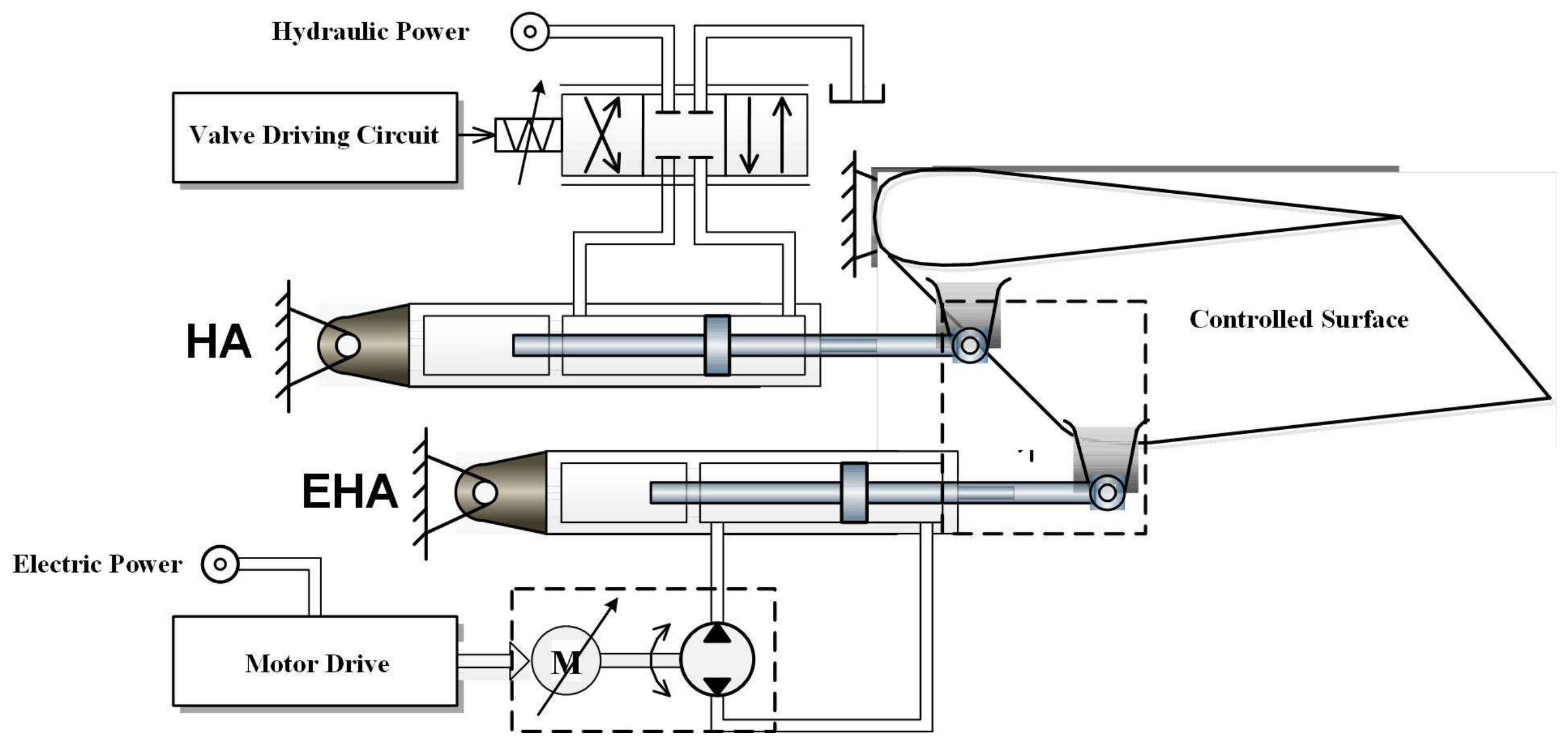
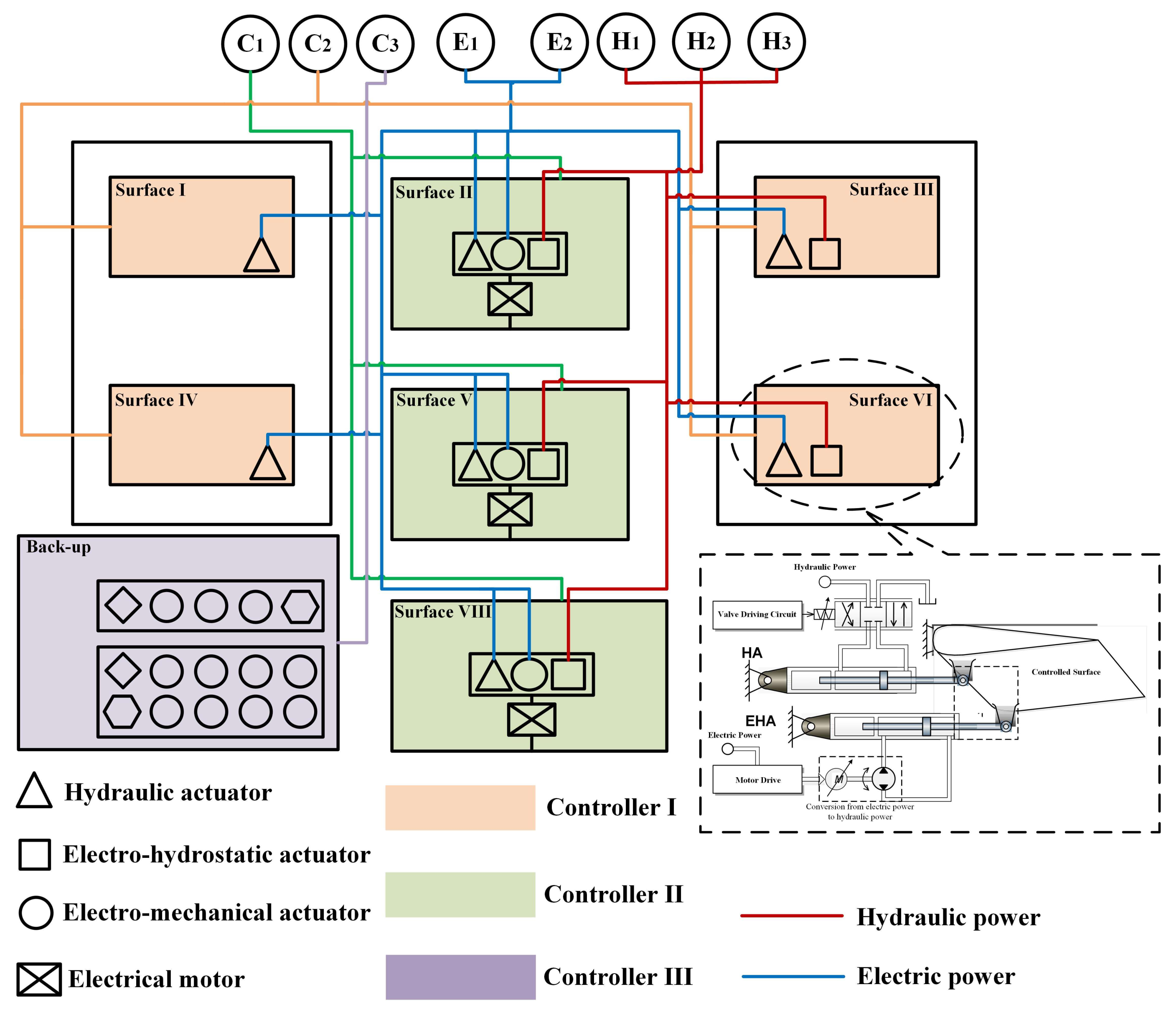
2.2. Redundant Configuration of Actuation System

The more electric control of safety critical systems not only requires the high-precision performance but also requires extremely high reliability and safety. Thus, redundant designs are often adopted, such as dual-redundant actuators and triple-redundant actuators. In order to integrate the advantages of hydraulic power and electric power, the typical isomorphic actuation system and heterogeneous actuation system shown in Figure 2, Figure 3 and Figure 4 are used in real-world applications. In an aircraft, the HA/HA, HA/EHA, and HA/EMA are classic dual-redundant actuation systems, as shown in Figure 2, Figure 3 and Figure 4.

Generally, the regulation of a dissimilar redundant actuator is to design the different actuator powered by a different power supply for one surface. In such design, when any actuator or power supply system fails, the other can fulfill the task through fault switching.

Table 1. Typical configuration of dissimilar redundant actuation system.

Redundancy	Actuator Type	Power Supply
Dual redundancies	HA, HA	Hydraulic power
	HA, EMA	Hydraulic and electric power
	HA, EHA	Hydraulic and electric power
Triple redundancies	HA, EHA, and EMA	Hydraulic and electric power

presents the typical configuration of a dissimilar redundant actuation system.

Remark 1.

Triple redundancy was considered in this research because when the number of redundancies increases, the performance indicators of an MECS will increase accordingly, which is not beneficial for system operation. Besides, an actuation system with more than three redundancies is rarely used in practice.

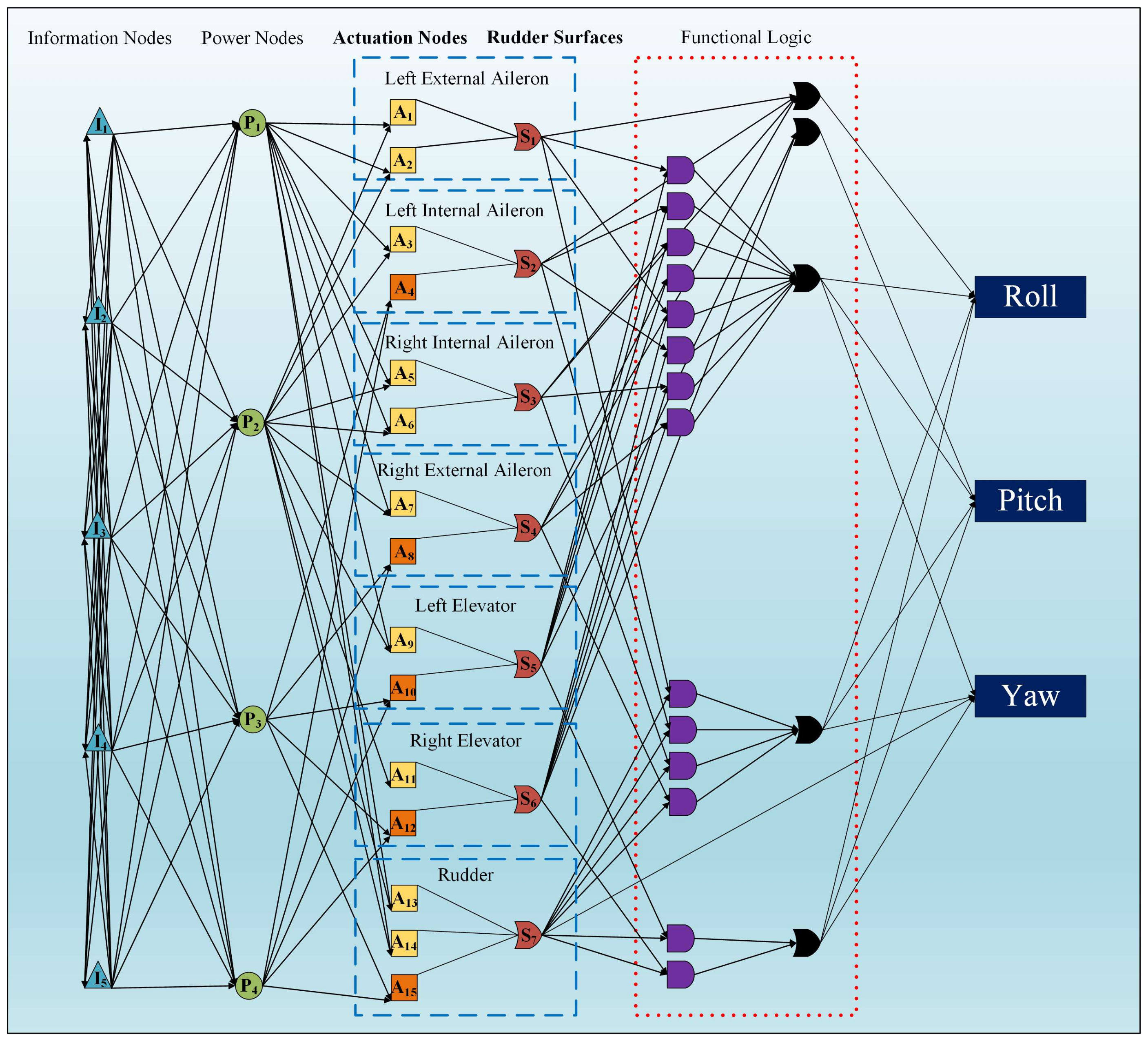
2.3. Redundant Configuration of More Electric Control System

As mentioned above, dissimilar redundancy technology is widely used in safety critical system design in order to improve system reliability. In a commercial aircraft, various controllers, actuators, and power supplies are applied in the aircraft actuation system. A typical redundant actuation system configuration based on high reliability for a commercial aircraft is illustrated in Figure 5. Although multiple control computers, actuators, and power supply systems can achieve high reliability, weights and costs will increase correspondingly, with maintainability decreased as well. Therefore, it is imperative to optimize the quantity of redundant control computers, power supply systems, and actuators. At same time, designers have to solve the common faults of dissimilar power supplies and dissimilar actuators as shown in Figure 2, Figure 3 and Figure 4.

In Figure 5, $I$ expresses the information nodes of the control computer; $P$ describes the power supply nodes; $A$ is the actuator nodes; and $S$ shows the surface of the aircraft. Herein, the actuator includes an HA, EHA, and EMA, as shown in Figure 2, Figure 3 and Figure 4. Both the fonts of actuation nodes and rudder surfaces are bold since they are our main considerations.

Definition 1.

Power supply module set is $P=\left\{P_i\right\}(i=1,2,\dots ,n)$. For aircraft shown in Figure 5, $P_1=H$means the power supply; $P_1$is the hydraulic power; and $P_2=E$means that the power supply $P_2$is electric power.

Definition 2.

Actuator module set is $A=\left\{A_j\right\}(j=1,2,\dots ,m)$. For aircraft shown in Figure 5, $A_1=HA$means that the actuator $A_1$is a hydraulic actuator. $A_2=EHA$means that the actuator $A_2$is an electro-hydrostatic actuator, and $A_3=EMA$means that the actuator$A_3$is a mechatronic actuator.

Remark 2.

Here, the commercial aircraft redundant actuation system is introduced as a typical MESC merely. In fact, our method is extensible and can be applied to more kinds of systems. In Section 4, we abstract a typical MECS with 3 hydraulic power supplies and 2 electric power supplies as the research object, which can be also extended to more combinations.

3. Multi-Objective Optimization of MECS Based on NSGA-II and AHP

Though an MECS can improve system reliability and ensure safety, when the system structure is more sophisticated, the corresponding structural indicators such as weight and cost will increase enormously. The design of an MECS may also increase the system volume and faults derived from the heavy weight. Therefore, we need to optimize factors such as the weight, power dissipation, and reliability of an MECS to ensure a compromise between these indicators.

3.1. Multi-Objective Optimization Modeling of MECS

The primary task for optimization design is to transfer the optimization problem into mathematical descriptions. Generally, an optimization problem is composed of three elements: objective functions, decision variables, and constraint conditions. The optimization problem of an MECS can be expressed as

$$\begin{array}{c}J=\max R_s(t)\\ R_s(t)=f(H_i,E_i,H{A}_j,EH{A}_j,EM{A}_j)\\ s.t.0\le m(H_i,E_i,H{A}_j,EH{A}_j,EM{A}_j)\le M\\ 0\le \psi (H_i,E_i,H{A}_j,EH{A}_j,EM{A}_j)\le \Psi \\ 0\le c(H_i,E_i,H{A}_j,EH{A}_j,EM{A}_j)\le C\\ ⋮\\ 0\le g(H_i,E_i,H{A}_j,EH{A}_j,EM{A}_j)\le G\\ i\in =ℒ=\{1,\dots ,m\}\subset \mathbb{N}\\ j\in =ℱ=\{1,\dots ,n\}\subset \mathbb{N}\end{array}$$

(1)

where function $J$ is the maximum reliability; $m(H_i,E_i,H{A}_j,EH{A}_j,EM{A}_j)$ is the actual evaluation mass of the MECS; $M$ is the superior limit of mass; $\psi (H_i,E_i,H{A}_j,EH{A}_j,EM{A}_j)$ expresses the actual evaluation power dissipation of the MECS; $\Psi$ is the superior limit of power dissipation; $c(H_i,E_i,H{A}_j,EH{A}_j,EM{A}_j)$ describes the actual evaluation cost of the MECS; $c$ represents the superior limit of cost; $g(H_i,E_i,H{A}_j,EH{A}_j,EM{A}_j)$ represents the other actual evaluation indicators of MECS; and $G$ represents the superior limit of other indicators. The specific evaluation methods of objective functions and constraints are given below.

3.1.1. Objective Function

According to Equation (1), reliability is the most essential indicator and the objective function. System reliability refers to the ability of the system to meet the specified functions within the specified time and under the specified conditions. Only when specific functions of an MECS are controlled effectively at the same time can the overall function of the system be guaranteed. Therefore, the overall functional reliability of an MECS is defined as the ability to effectively control the specific functions simultaneously within the specified time and under the specified conditions.

Based on the definition above and by considering an MECS with eight actuation functions, the functional reliability of an MECS can be expressed as

$$R_S=\mathrm{Pr}\left\{F_1\cap F_2\cap \cdots \cap F_8\right\}=\mathrm{Pr}\left\{S\right\}$$

(2)

where $F_1,\dots ,F_8$ represent the pivotal functions that MECS should accomplish.

By considering the multiple control surface combinations involved in the realization of system functions, Equation (2) can be rewritten as

$$R_S=\mathrm{Pr}\left\{\left(\underset{x=1}{\overset{p}{{\displaystyle \cup }}}{F}_1\right)\cap \left(\underset{y=1}{\overset{q}{{\displaystyle \cup }}}{F}_2\right)\cdots \cap \left(\underset{z=1}{\overset{m}{{\displaystyle \cup }}}{F}_8\right)\right\}$$

(3)

where $\left(\underset{x=1}{\overset{p}{{\displaystyle \cup }}}{F}_1\right)\cap \left(\underset{y=1}{\overset{q}{{\displaystyle \cup }}}{F}_2\right)\cdots \cap \left(\underset{z=1}{\overset{m}{{\displaystyle \cup }}}{F}_8\right)$ represents a certain combination that realizes the pivotal functions.

To simplify the calculation, the program first calculated the overall reliability of electric power supplies $E_1,E_2$ and then calculated the overall reliability of hydraulic power supplies $H_1,H_2$. Next, we calculated the minimum path and the program performing disjoint operation. Through decoupling analysis, nine minimal paths were obtained. Consequently, the functional reliability of an MECS can be calculated by

$$\begin{array}{l}{R}_S=\mathrm{Pr}\left\{\underset{i=1}{\overset{9}{{\displaystyle \cup }}}{S}_i\right\}=q_{E1}{q}_{E2}{q}_{E5}{q}_{E6}{p}_{EB}{p}_{ED}{p}_{EH}{p}_{EJ}{p}_{EN}{p}_{EO}{p}_{EP}{p}_{EQ}{p}_{ER}{p}_{ES}{p}_{ET}{p}_{EU}\\ p_{EV}{p}_{EW}{p}_{EX}{p}_{H1}{p}_{H3}{p}_{P1}{p}_{P2}{p}_{K1}{p}_{K2}{p}_{DD}{p}_{YY}{p}_{C1}{p}_{C2}{p}_{C3}+q_{E1}{p}_{E2}{q}_{E5}{q}_{E6}{p}_{EB}{p}_{ED}{p}_{EH}\\ p_{EJ}{p}_{EN}{p}_{EO}{p}_{EP}{p}_{EQ}{p}_{ER}{p}_{ES}{p}_{ET}{p}_{EU}{p}_{EV}{p}_{EW}{p}_{EX}{p}_{H3}{p}_{P1}{p}_{P2}{p}_{K1}{p}_{K2}{p}_{DD}{p}_{YY}{p}_{C1}{p}_{C2}\\ p_{C3}+\cdots +q_{E1}{p}_{E2}{p}_{E5}{p}_{EB}{p}_{ED}{p}_{EH}{p}_{EJ}{p}_{EN}{p}_{EO}{p}_{EP}{p}_{EQ}{p}_{ER}{p}_{ES}{p}_{ET}{p}_{EU}{p}_{EV}{p}_{EW}{p}_{EX}\\ p_{H1}{p}_{H3}{p}_{P1}{p}_{P2}{p}_{K1}{p}_{K2}{p}_{DD}{p}_{C1}{p}_{C2}{p}_{C3}+p_{E1}{p}_{E5}{p}_{EB}{p}_{ED}{p}_{EH}{p}_{EJ}{p}_{EN}{p}_{EO}{p}_{EP}{p}_{EQ}{p}_{ER}\\ p_{ES}{p}_{ET}{p}_{EU}{p}_{EV}{p}_{EW}{p}_{EX}{p}_{H1}{p}_{H3}{p}_{P1}{p}_{P2}{p}_{K1}{p}_{K2}{p}_{DD}{p}_{C1}{p}_{C2}{p}_{C3}\end{array}$$

(4)

Remark 3.

Equation (4) gives the relationship between system reliability and component system. In fact, system reliability is determined by each component reliability, that is, the actuator reliability, while actuator reliability is associated with weight, power consumption, and cost. These indicators will eventually have an influence on system reliability.

3.1.2. Constraint Conditions

The aim of optimization design is to identify the optimal solution from the practical solutions. The optimal solution can meet the goal of design as far as possible. The elevation of weight will restrict the MECS installation power; hence, weight is a vital index for system property. Power dissipation is another vital property index. In the optimization design of an MECS, particularly for a highly-efficient MECS, how to decrease the power dissipation with the existent technology and apparatus is a challenge which need to be tackled by designers. Meanwhile, as an MECS has to harbor high performance and reliability, so the reliability of an MECS should be considered. For practical application, the cost is an indispensable indicator that must be evaluated. Eventually, weight, power dissipation, cost, and reliability are determined as constraint conditions.

• Weight

Weight is a vital evaluation index and decisive factor of an MECS. When we evaluate weight, the difficulties usually include various components, many of which exhibit a nonlinear growth relationship with design requirements, and serious coupling with other systems with different types of actuators. For an EHA, since it consists of the integration block, cylinder, pump, and motor, its weight evaluation can be presented as

$$M_{EHA}=M_{block}+M_{cylinder}+M_{pump}+M_{motor}$$

(5)

where $M_{block},M_{cylinder},M_{pump}$ refer to the weight of the integration block, cylinder, and pump, respectively. $M_{motor}$ denotes the weight of the brushless direct-current motor (BLDC). All of them have the same unit, kilograms.

A permanent magnet brushless direct-current motor (BLDC) is utilized in the EHA due to its satisfactory control property and great power-to-mass ratio. The weight forecast of the BLDC is expressed by

$$M_{motor}=0.628T^{3/3.5}+0.783$$

(6)

in which $T$ represents the torque of BLDC.

The pump weight is proportionate to pump output. Thus, $M_{pump}$ can be expressed as [33]

$$M_{pump}=0.339D+2.038$$

(7)

The integration block is the EHA frame and involves the indispensable parts such as the nonreturn valve, filter, and accumulator. The overall weight is speculated by the EHA power, which is expressed as [33]

$$M_{block}=0.105P_{EHA}+2$$

(8)

where $P_{EHA}$ denotes the maximal power of EHA.

The fluid cylinder weight includes the four parts stated below:

$$M_{cylinder}=M_{cover}+M_{shell}+M_{piston}+M_{rod}$$

(9)

where $M_{cover},M_{shell},M_{piston},M_{rod}$ are the weights of the cylinder cover, shell, piston, and plunger rod, respectively. All of them can be calculated by

$$\left\{\begin{array}{l}{M}_{rod}=\frac{\pi }{4}\times d_{rod}^2\times L_{rod}\times {\rho }_{steel}\hfill \\ M_{piston}=A\times t_{piston}\times {\rho }_{copper}\hfill \\ M_{shell}=\frac{\pi }{4}\times \left(d_{shell}^2-\frac{4A}{\pi }\right)\times L_{shell}\times {\rho }_{steel}\hfill \\ M_{cover}=2\times \frac{\pi }{4}\times d_{shell}^2\times t_{cover}\times {\rho }_{steel}\hfill \end{array}\right.$$

(10)

Thus, the total weight can be evaluated as

$$M={\displaystyle \sum _{i=1}^{n_{HA}}{M}_{HA}+}{\displaystyle \sum _{i=1}^{n_{EHA}}{M}_{EHA}+}{\displaystyle \sum _{i=1}^{n_{EMA}}{M}_{EMA}+}{M}_{elec}+M_{pipe}+M_{wire}$$

(11)

where $M_{HA},M_{EHA},M_{EMA}$ represent the weights of HA, EHA, and EMA, respectively, and $M_{elec},M_{pipe},M_{wire}$ represent the weights of electric equipment, pipe and wire, respectively.

• Power efficiency

For an EHA, the motor converts electric energy to hydraulic power, pushing the cylinder to realize the movement of the control surface. For an EHA system, when its control surface load is certain, it saves more energy, resulting in lower power dissipation. The control surface torque $T_S$, control surface velocity ${\omega }_S$, and pressure $P_S$ are known design specifications. The aim of decreasing the power dissipation of an EHA is to decrease the power output of the motor $P$, which is written as

$$P=T\times W$$

(12)

The motor is directly connected to the pump, so the torque and speed of the motor and pump are the same. The torque of the pump is expressed as

$$T=J_{pm}\times \frac{d\omega }{dt}+K_{fric}\times \omega +(p_f+2p_{pipe})\times \frac{D}{2\pi }$$

(13)

where $J_{pm}$ is the pump rotational inertia; $K_{fric}$ denotes the viscosity factor, $J_{pm}\times d\omega /dt=0$; the pump rotation velocity is constant; $p_f$ denotes the differential pressure between the 2 cylinder cavities; and $p_{pipe}$ denotes the pressure consumption within the pipe. Hence, Equation (13) is written as

$$T=K_{fric}\times \omega +(p_f+2p_{pipe})\times \frac{D}{2\pi }$$

(14)

in which $p_f=F/A$, $F$ is the loading force of an EHA and $A$ denotes the piston effective area, which can be calculated by

$$A=\frac{kF}{P_S}$$

(15)

in which $k>1$ denotes a logical excess margin, and $F$ can be described by

$$F=\frac{T_S\times \sin (\theta +{30}^{°})}{L}$$

(16)

For an EMA, the power dissipation is determined by the ball screw. Therefore, Equation (17) gives the calculation method for the drive torque of the ball screw:

$$T_a=\frac{F_a\times I}{2\pi \times n_1}$$

(17)

where $T_a$ represents the drive torque; $I$ is the lead screw; $n_1$ is the positive efficiency of the feed screw; and $F_a$ refers to the axial load, which can be expressed by

$$F_a=F+\mu mg$$

(18)

where $F$ means the axial cutting force of the lead screw, $\mu$ is the comprehensive friction coefficient, and $m$ refers the weight of the worktable and workpiece.

After the calculation of the drive torque $T_a$, the motor power can be determined accordingly; thus, the corresponding power dissipation of the motor can be obtained.

For the power dissipation evaluation of a HA, the volumetric efficiency of the pump ${\eta }_0$ is the main affecting factor, which can be described by

$${\eta }_0=\frac{Q}{Q_0}\times 100\%$$

(19)

where $Q_0$ means the theoretical flow of the pump, and $Q$ is the actual pump flow, which is written as

$$Q=Q_{pump}+Q_{pipe}+Q_{cylinder}$$

(20)

where $Q_{pump}$ denotes the pump leak, $Q_{pipe}$ denotes the loss of flow within the hydraulic tube, and $Q_{cylinder}$ denotes the cylinder flow.

$$\left\{\begin{array}{l}{Q}_{pump}=\xi \times (p_1-p_2)=\xi \times F/A\\ Q_{cylinder}=A\times v\\ Q_{pipe}=2\times \xi \times p_{pipe}\end{array}\right.$$

(21)

where $\xi$ is the pump leakance coefficient, $p_{pipe}$ denotes the pipe pressure drop, and $v$ denotes the cylinder speed.

• Cost

For an MECS, cost is another index worthy of consideration. In this paper, the total costs are divided into two parts:

$$C=C_{manu}+C_{oper}$$

(22)

where $C$ represents the total cost of an MECS, $C_{manu}$ refers to the manufacturing cost, and $C_{oper}$ represents the operation cost.

However, when we evaluated the total cost, the component cost exhibited a nonlinear growth relationship with the requirement. To simplify this process, this paper utilized different configurations to obtain the costs of all components. In the evaluation of manufacturing costs, the main components considered included the HA, EHA, EMA, oil boxes, pipelines, cables, engine-driven pump (EDP), and electric motor driven pump (EMP). The evaluation was conducted mainly based on the similarity principle. Thus, the manufacturing costs is expressed as

$$C_{manu}={\displaystyle \sum _{i=1}^{n_{edp}}{C}_{edp}}+{\displaystyle \sum _{i=1}^{n_{emp}}{C}_{emp}}+{\displaystyle \sum _{i=1}^{n_{tank}}{C}_{tank}}+{\displaystyle \sum _{i=1}^{n_{motor}}{C}_{motor}}+{\displaystyle \sum _{i=1}^{n_{act}}{C}_{act}}+{\displaystyle \sum _{i=1}^{n_{pipe}}{C}_{pipe}}+{\displaystyle \sum _{i=1}^{n_{wire}}{C}_{wire}}$$

(23)

where $C_{edp}$ represents the cost of the EDP; $C_{emp}$ refers to the cost of the EMP; $C_{tank}$ is the cost of the tank; $C_{motor}$ is the cost of the motor; $C_{act}$ describes the cost of the actuator; $C_{pipe}$ expresses the cost of the pipe; and $C_{wire}$ denotes the wire cost.

The operation expense primarily denotes the Direct Operating Costs (DOCs), which are changeable costs directly derived from operating the aircraft [34]. The fuel expense and maintenance expenditure of DOCs are changeable. Hence, the DOCs are predominantly related to fuel expense and maintenance expenditure herein. The operation expense speculation is written as

$$C_{oper}=C_{oil}+C_{main}$$

(24)

where $C_{oil}$ and $C_{main}$ represent the fuel cost and maintenance cost, respectively.

Based on the statistical proportion of main flight control maintenance cost in the total maintenance expenditure, the fuel expense speculation primarily considers the fuel consumption during the life of the commercial aircraft. The function of fuel cost with respect to time is expressed as

$$C_{oil}(t)=50\times C_0\times Weight\times ({1.02}^t-1)$$

(25)

where $C_0$ means the average annual fuel cost of the aircraft and $Weight$ represents the fuel weight.

The maintenance cost of the aircraft in the whole life cycle mainly has two parts [35]. One is called the cyclic cost $C_C$, which is related to the take-off and landing of the aircraft, such as the maintenance of its braking device, flap system, and landing gear. The other cost is related to the flight time of the aircraft, such as the regular loss and replacement of parts caused by each hour of flight. This part of the cost is called hourly cost $C_H$. The evaluation of the maintenance cost is usually accomplished through the statistic of man-hour cost. Equation (26) provides the method for man-hour cost calculation

$$C_{main}=C_H\times t+C_C\times t+M\times (1/\alpha )\times R\times t$$

(26)

3.1.3. Design Variables

The expression of a goal suggests that there are substantial that which ought to be identified in configuration designs. Nevertheless, considering all those variables during optimization makes convergence difficult and is quite time-consuming. Hence, merely vital variables having a remarkable influence on MECS property ought to be optimized. Overall, the selective principles of the design variates are stated below:

• The quantity of design variates ought to be decreased to the utmost extent. Overall, the quantity of design variates in mechanical optimization design should not surpass 5.
• The variables ought to exert a remarkable impact on the goal function. Indexes affecting the constraint and property directly ought to be chosen as design variates.
• The chosen variates ought to be independent.
• The variates ought to be chosen as per the optimization goal.

According to the aforesaid principles, the optimization variates are chosen via:

$$x=\left\{\begin{array}{c}{x}_1\\ x_2\\ x_3\end{array}\right\}=\left\{\begin{array}{c}{n}_{HA}\\ n_{EHA}\\ n_{EMA}\end{array}\right\}$$

(27)

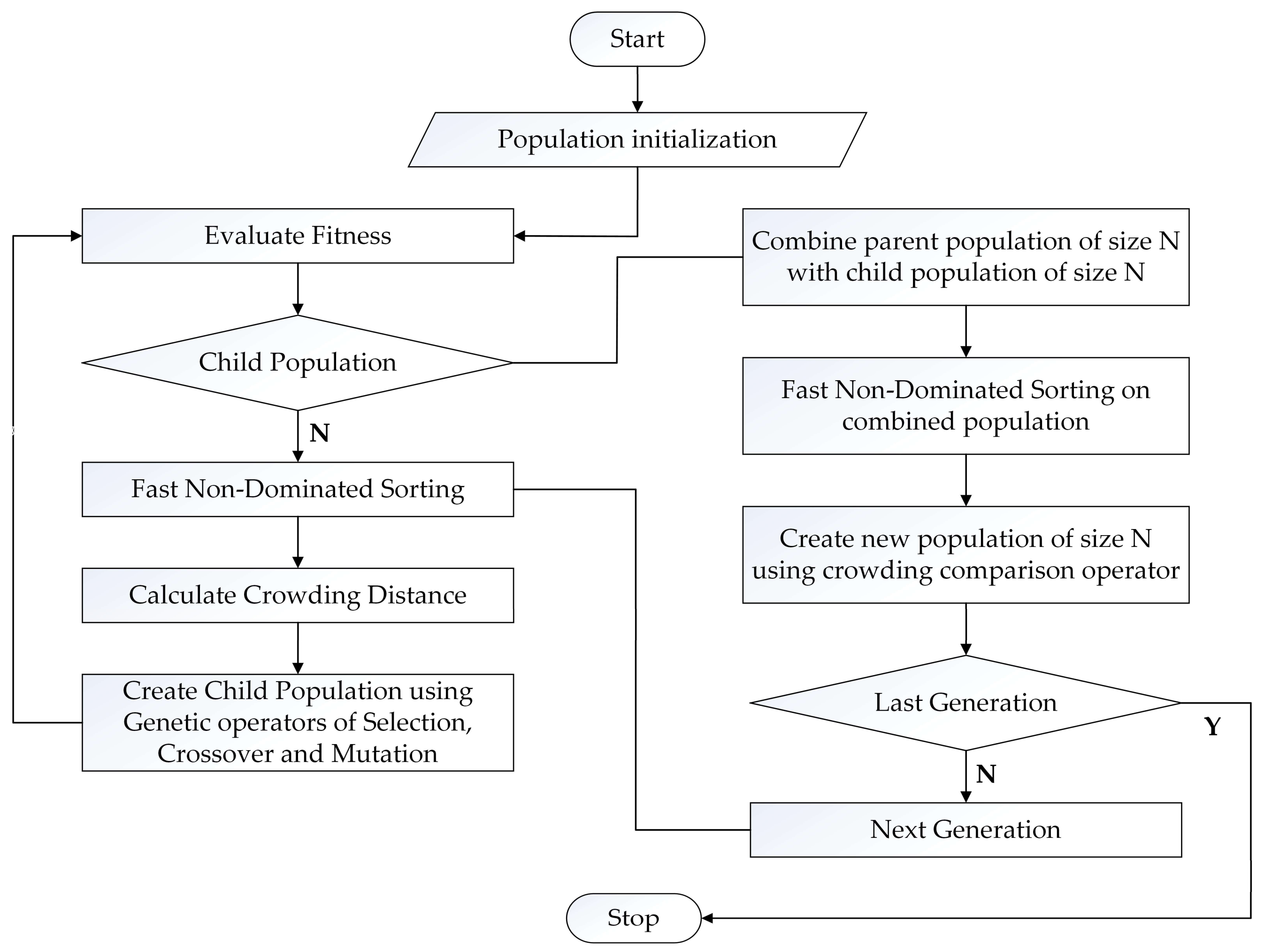
3.2. Multi-Objective Optimization Based on NSGA-II

The optimization issue herein aimed at the configuration design of an MECS. NSGA-II is proper for optimizing multi-objective issues as it exhibits strong distributed capability and rapid convergence. The flow chart of NSGA-II is shown in Figure 6. Subsequently, the encoding/decoding mode and fast non-dominated sorting process are elaborated.

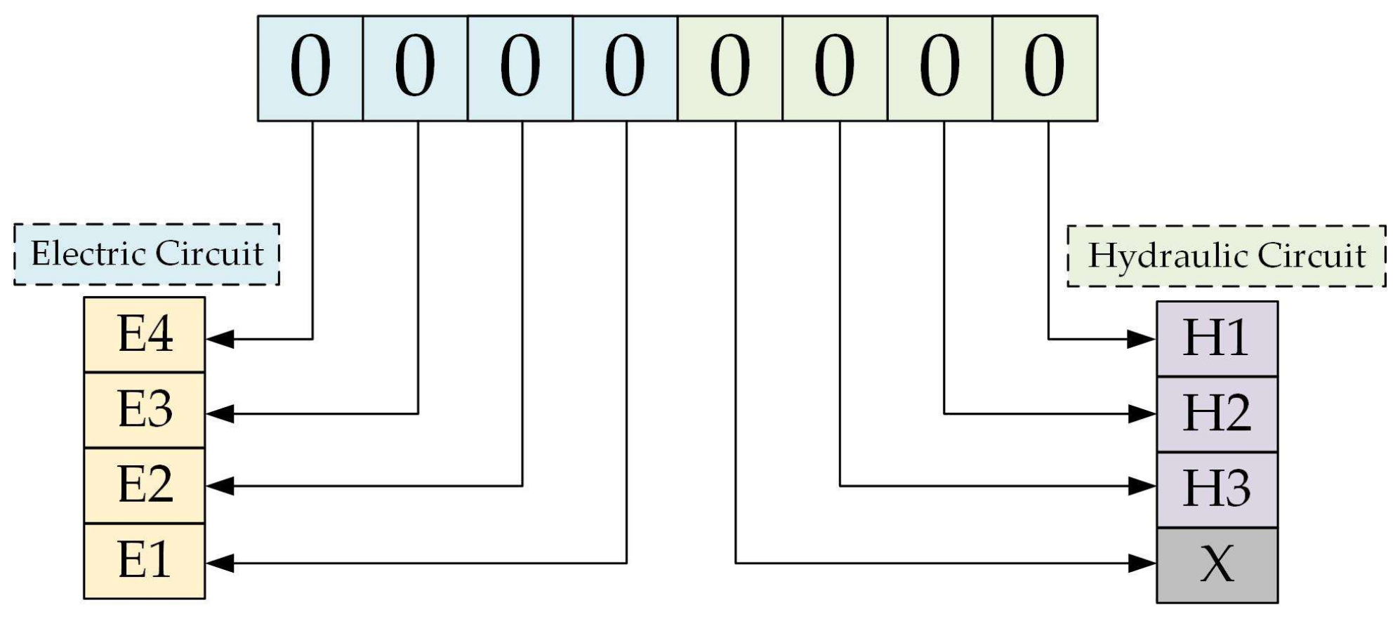
3.2.1. Encoding and Decoding

In our research, the binary encoding mode was adopted in NSGA-II, which was simple, efficient, and easy to design and use for implementing crossover and mutation operations. Two types of energy information were encoded through this mode, while the configuration of each actuation system was also expressed in binary. Figure 7 illustrates this coding mode.

3.2.2. Fast Non-Dominated Sorting

Compared with non-dominated sorting approach utilized in NSGA arithmetic, the rapid non-dominated sorting utilized in NSGA-II algorithm requires lower computational complexity, which is only about $O(M{N}^2)$. The overall algorithm flow was presented as follow:

Algorithm 1: Fast non-dominated sorting

1:    Fast-non-dominated-sort ($P$)

2:     for each $p\in P$ 3:      for each $q\in P$ 4:       if $p{\le }_{n}q$, then     # if $p$ is dominated by $q$, then add $q$ to $S_p$ 5:        $S_p=S_p\cup q$ 6:       else if $q{\le }_{n}p$, then 7:        $n_p=n_p+1$ 8:      if $n_p=0$, then 9:        $p_{rank}=1$, $F_1=F_1\cup P$    # when $n_p$ of the individual is 0, then this individual is the first level of Pareto 10:    The comparison of dominating relationships between individuals, $S_p$ and $n_p$, are introduced for storage and records, respectively; ${\le }_n$ represents the comparison of dominating relationships. The solution of $n_p=0$ is stored in the records of level 1, and the solution of level 1 has higher priority than that of level 2. 11:    i = 1. 12:    while $F_i=\varnothing$ do 13:    H=$\varnothing$ 14:    for each $p\in F_i$ 15:     for each $q\in S_p$        # Sort all the individuals in $S_p$ 16:      $n_q=n_q-1$ 17:       if $n_q=0$, then       # when $n_q$ of the individual is 0, it is a non-dominated individual 18:         $q_{rank}=i+2,H=H\cup q$ # The Pareto level of this individual is the current highest level plus 1. At this moment, the initial value of i was 0, so we added 2. 19:    end while 20:    $i=i+1,F_i=H$ 21:    Loop the program to obtain level 2, level 3… The computational complexity is $O(M{N}^2)$

3.2.3. Crowding Degree Calculation

Crowing degree $I_d$ refers to the local crowding distance between any two adjacent points whose level are the same in the target space. The purpose of introducing crowding degree is to improve the distribution uniformity of the Pareto solution set. Furthermore, it could not only boost the diversity of population but also enhance system robustness. The crowding degree $I_d$ could be expressed as the length of the maximum rectangle of individual $i$ on both sides, where the rectangle only includes $i$ itself.

The main procedure to determine the degree of individual congestion involves three steps:

• Define the crowding degree of every individual in population $i$ as $I_d=0$;
• Define the crowding degree $0_d$ and $i_d$ of boundary individuals as $\infty$ according to each evaluation indicator;
• Define the crowding degree of marginal individuals as a larger number $L{(1)}_d=L{(l)}_d=M$ to prioritize individuals on the sorting edge; thus, the crowding degree of any other individual $I_d$ can be expressed as

$$I_d={\displaystyle \sum _{j=1}^m\left(\left|f_j^{i+1}-f_j^{i-1}\right|\right)}$$

(28)

where $j$ refers to each evaluation indicator; $f_j^{i+1}$ represents the $jth$ evaluation indicator value of individual $i+1$; and $f_j^{i+1}$ represents the $jth$ evaluation indicator value of individual $i-1$.

Through the aforesaid steps and calculation, every individual was endowed with two attributes, i.e., the crowding distance and the rank. This laid the foundation for the follow-up processes.

3.2.4. Optimal Selection

The optimal selection avoids the loss of effective factors and ensures the survival rate of high-performance individuals, so it can ensure that the Pareto optimal solution is continuously optimized. The optimal selection can not only improve the efficiency and convergence of the optimization but also ensure the uniformity of the optimization process. The selection process is completed by comparing the results of fast non-dominated sorting and crowding calculation, and better individuals are selected after comparison. Two steps are involved during this process.

• The first step is the rank comparison. Select two individuals $a$ and $b$ randomly and make comparison between $A_{rank}$ (the non-dominated rank of individual $a$) and $B_{rank}$ (the non-dominated rank of individual $b$). When $A_{rank}<B_{rank}$, $a$ is better than $b$ and vice versa. Moreover, the crowding degree requires to be compared when $A_{rank}=B_{rank}$;
• The second step is the crowding degree comparison. When condition $A_d>B_d$ is satisfied, it indicates that individual $a$ is better; otherwise, individual $b$ is better. Then, the better individual is selected to continue the following optimal processes.

3.2.5. Crossover

The main function of crossover is to simulate gene recombination in the process of heredity and evolution. There are various approaches to implement it, such as uniform crossover, multi-point crossover, and binary crossover. In our research, the simulated binary crossover is adopted for crossover operation, which is expressed as

$$\begin{array}{c}{y}_{1j}=0.5\times \left[\left(1+{\gamma }_j\right)x_{1j}+\left(1-{\gamma }_j\right)x_{2j}\right]\\ y_{2j}=0.5\times \left[\left(1-{\gamma }_j\right)x_{1j}+\left(1+{\gamma }_j\right)x_{2j}\right]\\ \left\{\begin{array}{c}{\left(2u_j\right)}^{\frac{1}{\eta +1}}if{u}_j\le 0.5\\ {\left(\frac{1}{2\left(1-u_j\right)}\right)}^{\frac{1}{\eta +1}}else\end{array}\right.\end{array}$$

(29)

where $u_j\in \left(0,1\right)$; $x_{1j}$ and $x_{2j}$ are parent individuals; $y_{1j}$ and $y_{2j}$ are offspring individuals; and $\eta >0$ refers to the cross-distribution index. Generally, $\eta =20$ is the best value of the cross-distribution index by default.

3.2.6. Mutation

Mutation is widely applied to simulate variation links in the process of biological heredity and evolution, which refers to the replacement between genes, that is, substitute the other gene values with the alleles on the locus to create new individuals. Through mutation, not only could the local searchability be improved but also the population diversity is guaranteed.

This paper introduced the polynomial mutation method into the research on multi-objective optimization problems. The form of mutation operator is expressed as

$$\begin{array}{c}{V}_k^{\prime }=V_k+\delta \left(u_k-L_k\right)\\ \delta =\left\{\begin{array}{l}{\left[2u+(1-2u){\left(1\mid -{\delta }_1\right)}^{{\eta }_m+1}\right]}^{\frac{1}{{\eta }_m+1}}-1ifu\le 0.5\hfill \\ 1-{\left[2(1-u)+2(u-0.5){\left(1-{\delta }_2\right)}^{{\eta }_m+1}\right]}^{\frac{1}{{\eta }_m+1}}elseifu>0.5\hfill \end{array}\right.\end{array}$$

(30)

where ${\delta }_1=\frac{\left(V_k-L_k\right)}{\left(u_k-L_k\right)},{\delta }_2=\frac{\left(u_k-V_k\right)}{\left(u_k-L_k\right)}$, $u$ denotes a stochastic number in interval [0,1], ${\eta }_m$ denotes the distribution index, and $V_k$ is a parent individual.

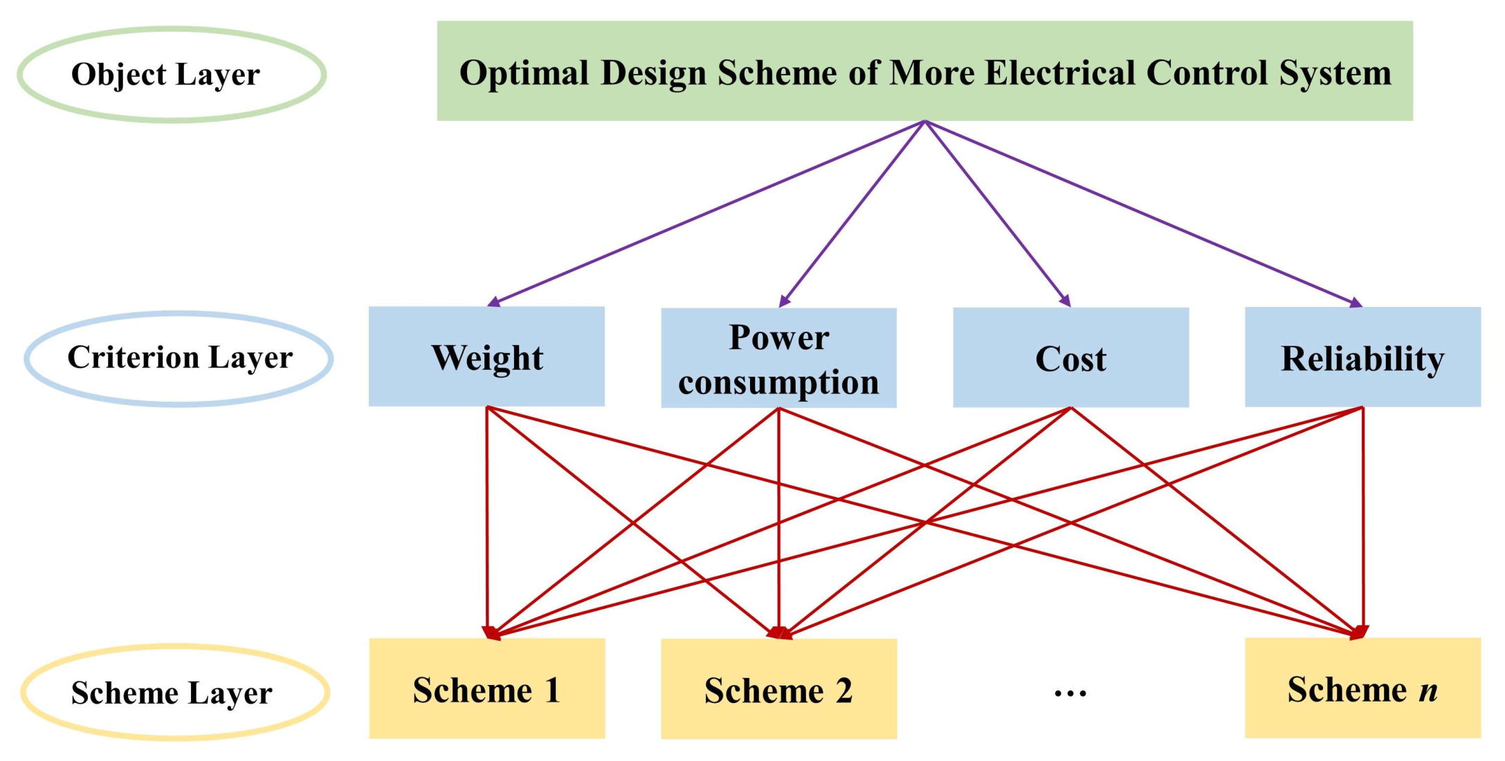
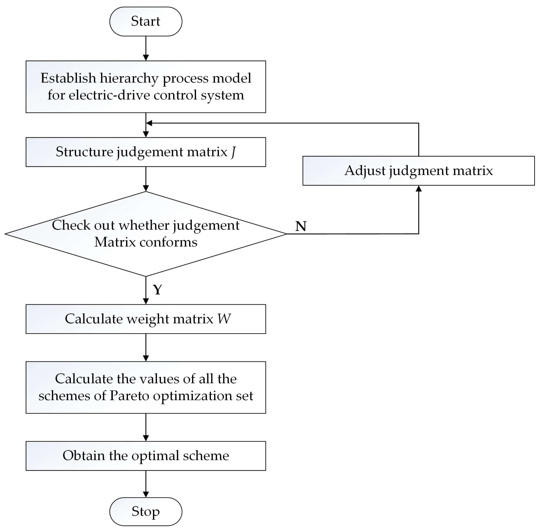
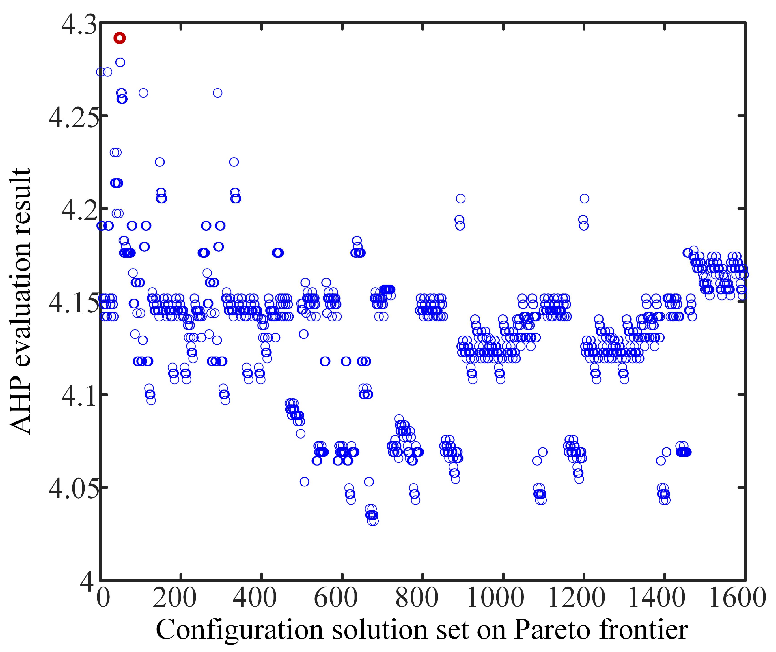
3.3. Comprehensive Evaluation of System Configuration Based on AHP

The analytic hierarchy process (AHP) is a multi-objective decision analysis approach that combines qualitation and quantitation analyses, where elements associated with task decisions are divided into the object level, criterion level and scheme level. The AHP mathematizes the decision-making via a few quantitation data based on deep analyses, such as the influential factors and inner association of the decision-making problems. AHP can offer an easy decision approach for intricate decision issues with several standards and no evident structure features. Questions to be evaluated in MECS optimization design ought to be methodized and layered, and the structure model of hierarchy analysis ought to be constructed. A three-level hierarchy structure of AHP was presented by Figure 8. Level 1 is the general objective of decision-making, which denotes the optimum design of MECS. Level 2 denotes the criterion layer, where the weight, power dissipation, expense, and dependability are utilized as evaluation standards of system multi-objective optimization design. Level 3 denotes the scheme layer, where the solutions are determined in the Pareto frontier acquired by NSGA-II. Besides, the process of AHP mainly includes the judgment matrix structure, weight coefficient calculation, consistency of judgment matrix verification, and weight coefficients of goal level calculation. The flow chart of AHP was shown in Figure 9.

• Construct the decision-making model for AHP according to Figure 8.
• Structure the judgement matrix $J$. Judgement matrix is established as per the association between the goals in the criterion layer.

$$J=\left[\begin{array}{cccc}1& 3& 9& 1\\ \frac{1}{3}& 1& \frac{1}{3}& \frac{1}{3}\\ \frac{1}{9}& \frac{1}{3}& 1& \frac{1}{9}\\ 1& 3& 9& 1\end{array}\right]$$

(31)

3.

Validate the judgement matrix coherence. Coherence index is computed via:

$$\left\{\begin{array}{c}CI=\frac{{\lambda }_{\max }-n}{n-1}\\ CR=\frac{CI}{RI}\end{array}\right.$$

(32)

where $CI$ denotes the coherence index of the judgment matrix, $RI$ denotes the average stochastic coherence index of the matrix (specific values were presented by

Table 2. Values of the average stochastic coherence index.

n	1	2	3	4	5	6	7	8	9
RI	0.00	0.00	0.58	0.90	1.12	1.24	1.32	1.41	1.45

), $CR$ denotes the stochastic coherence ratio of the matrix, ${\lambda }_{\max }$ denotes the maximal value of the matrix characteristic value, and $n$ denotes the matrix order.

By computation, if ${\lambda }_{\max }=3.7638$ and CI = (3.7638 − 4)/(4 − 1) = −0.0787, then CR = −0.0787/0.90 = −0.0875 < 0.1, which suggests that the weight matrix is coherent. When the consistence test is not met, return to step 2 and reconstruct the judgement matrix.

4.

Compute the weighted coefficient between the contrasted elements with the relevant standards. Compute the continued product $M_i$ of each row element in $A$, the product of every row element, and its n-th root ${\overline{w}}_1$.

$$\left\{\begin{array}{c} M_i={\prod }_{i=1}^n{x}_{ij}={\left[\begin{array}{cccc}27& 0.0370& 0.0041& 27\end{array}\right]}^T,i=1,\cdots ,n\\ {\overline{w}}_1=\sqrt[n]{M_i}={\left[\begin{array}{cccc}2.2795& 0.4387& 0.2533& 2.2795\end{array}\right]}^T,i=1,\cdots ,n\end{array}\right.$$

(33)

Normalize ${\overline{w}}_1$ as $W_i={\overline{w}}_1/{\displaystyle {\sum }_{i=1}^n{\overline{w}}_1}$, where $W_i$ denotes the weighted coefficient of every factor.

$$W=\left[\begin{array}{cccc}0.4341& 0.0835& 0.0482& 0.4341\end{array}\right]$$

(34)

5.

Speculate the design in the Pareto frontier as per the weighted coefficients of every standard, and afterwards get the optimum design of MECS.

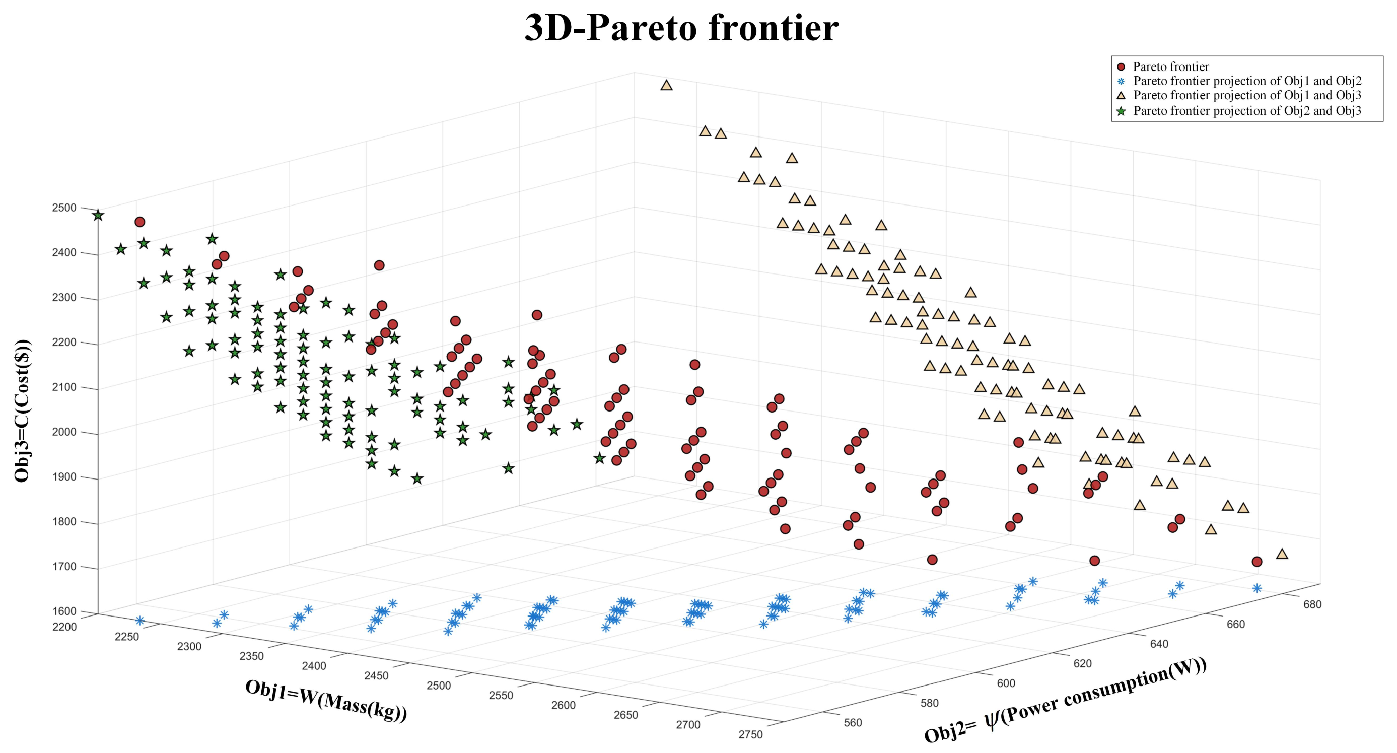
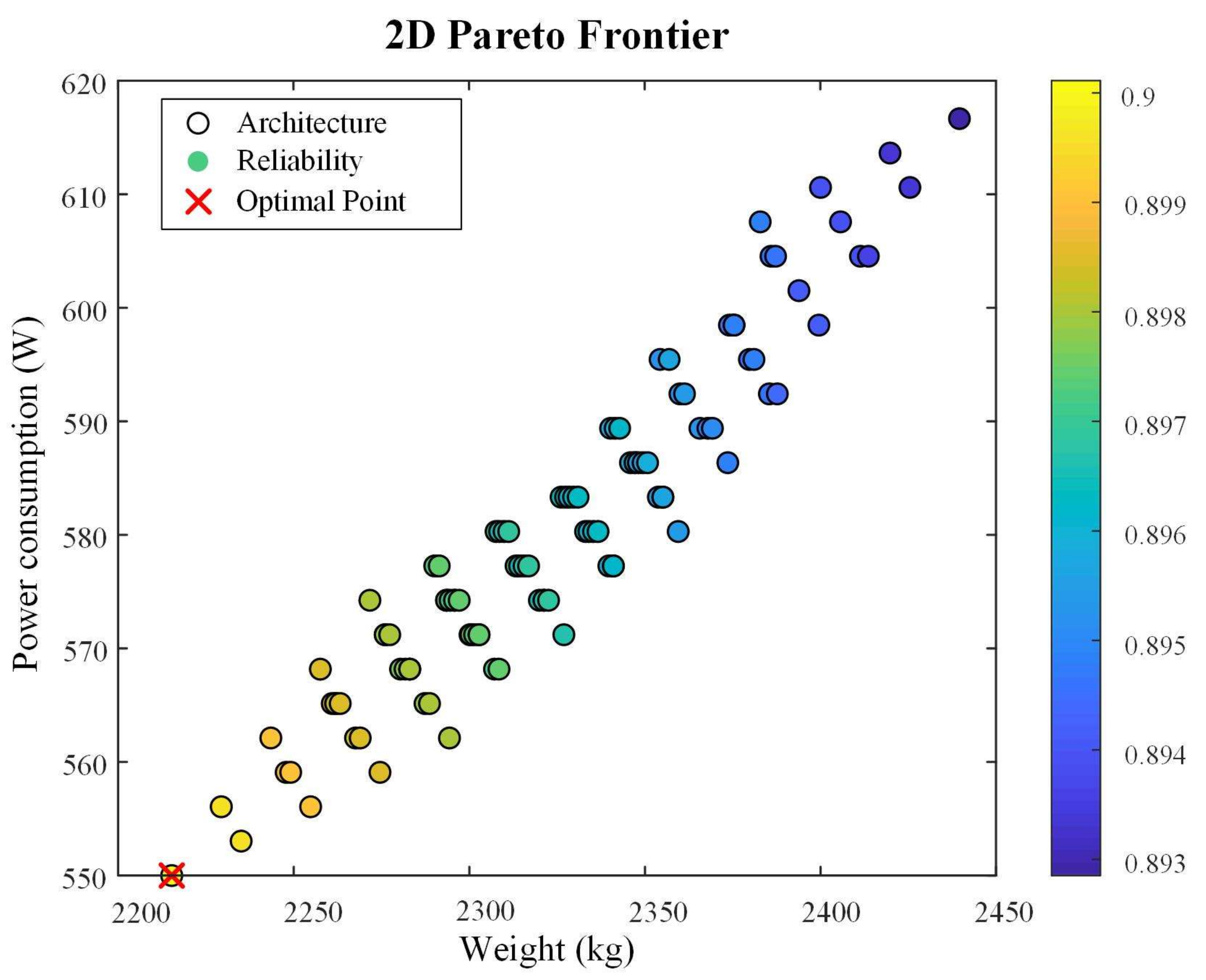
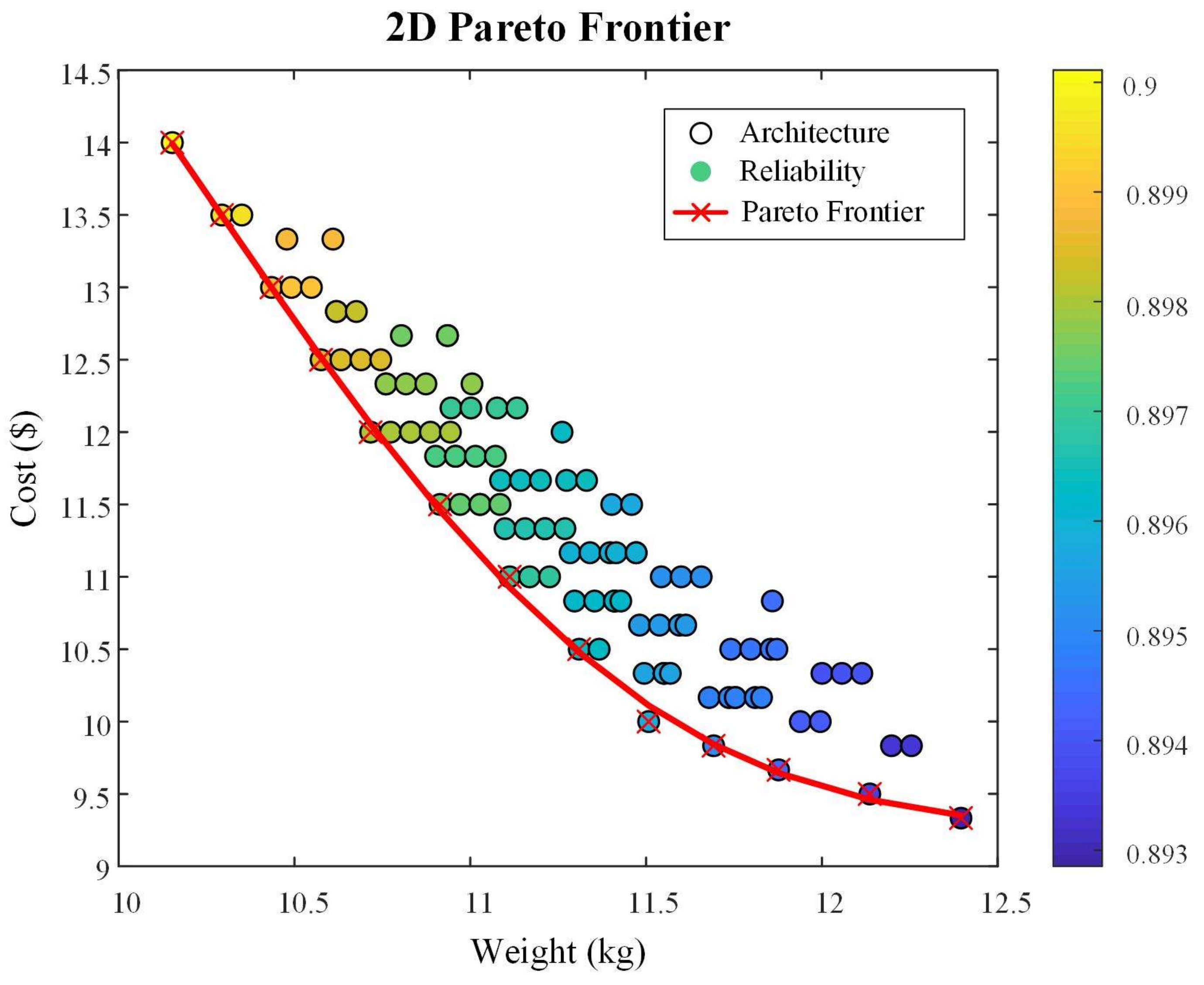
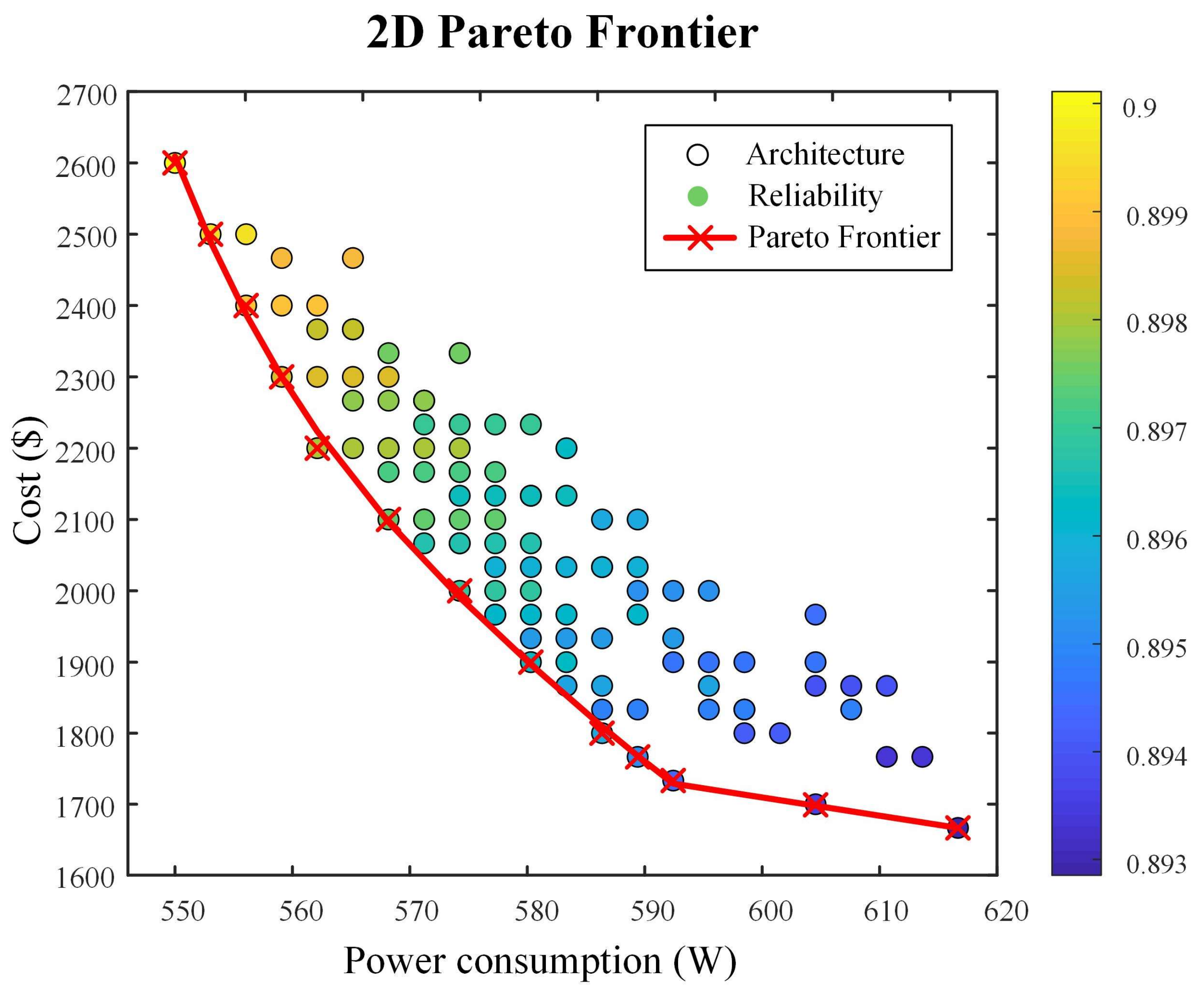
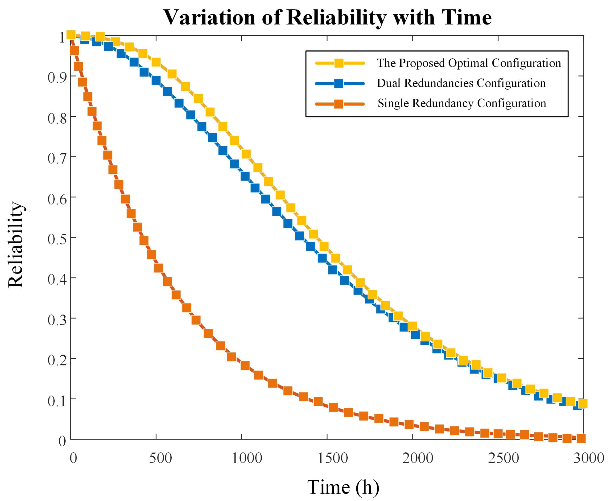
4. Case Study and Discussion

The diagram of an MECS with three fluid power supplies and two electric power supplies (3H2E) was presented by Figure 10. The tendency toward more electricity causes the transformation from hydraulic power into standby energy, or the replacement of hydraulic power with electrical energy, which produces more options for all control surfaces. For every actuator, it can be an HA linked to hydraulic source or an EHA linked to electrical source. In addition, each actuator is controlled by at least one controller. Therefore, the number of alternative configurations of the MECS is exceedingly high.

In this section, we introduced the proposed optimization method into the case study of the MECS illustrated in Figure 10. By setting the maximum optimization iterations of NSGA-II as 200, and population size as 500, we obtained the Pareto frontier of the optimization result illustrated in Figure 11. W refers to the weight of the MECS, $P$ is the power consumption of the MECS, and C represents the expense of the MECS. The red-round-dot-curved surface is a 3D Pareto optimum front curved surface. Every dot denotes an actuation design. The green line, marked by hollow pentagram; blue line, marked by cross symbol; and yellow line, marked by triangle were projected on three planes. The Pareto front was utilized to realize multi-objective optimization and to achieve a certain decrease in configuration quantity.

Moreover, the graph in Figure 11 presents the relationship among the three objectives. The line in x, y plane presents that weight and power have the relation of promotion. The line in x, z plane presents that weight and expense are contradictory. The line in y, z plane displays contradictory power and expense of an MECS. When the power decreases, the expense is elevated. The design objective is to minimize power and expense; hence, those two functions conflict with one another. Due to the conflicts between design indexes, it is hard to make each index optimum simultaneously.

In addition, to better illustrate the relationship between these three objectives and system reliability, we projected Figure 11 onto three 2-D planes, respectively, and obtained the 2D-pareto frontiers in Figure 12, Figure 13 and Figure 14. Reliability was used as the scale parameter to color different system configurations, i.e., the brighter the color, the higher the reliability.

Through multi-objective optimization, the Pareto optimization frontier was acquired. Nevertheless, finding the best way to identify the optimal solution in the Pareto frontier remains a daunting challenge. Thus, AHP was introduced to solve this problem. According to Section 3.3, diverse optimum solutions can be realized via structuring diverse judgment matrices when we use AHP to perform decision analyses. Thus, to better observe the association between the goals more, the judgment matrix was presented by

Table 3. The association between the objectives.

Objectives	Weight	Power Dissipation	Cost	Reliability
Weight	1	3	9	1
Power dissipation	1/3	1	1/3	1/3
Cost	1/9	1/3	1	1/9
Reliability	1	3	9	1

, and the eventual result was illustrated in Figure 15 and Figure 16.

Through a comprehensive analysis of AHP, the score of each solution on the Pareto frontier was acquired. The solution with the greatest score is the best one. As presented by Figure 15 and Figure 16, the optimal design strategy is number 96 of the Pareto frontiers, with triple redundancy configuration used in the MCES. The reliability of our designed configuration increased by 5.89% and 55.34% respectively, compared with the dual redundancy and single redundancy configurations. The results indicated that our approach combining multi-objective optimization and decision-making could realize the multi-objective optimization design of an MECS. The solutions on the Pareto frontier acquired by NSGA-II arithmetic were uniformly distributed, which suggested that we could offer designers more diversified choices. Subsequently, AHP was employed for the eventual decision analyses, which enabled designers to introduce predilections and experiences for different goals.

5. Conclusions and Future Work

The present research demonstrated the multi-objective optimization for an MECS. By designing the level length, the objectives are optimized. However, it is hard to minimize every goal simultaneously due to the conflicts between these objectives. Thus, an appropriate multi-objective optimization algorithm, which can compromise multiple objectives, is required to acquire the Pareto optimum solution set. Besides, since the Pareto frontier solution is not a solution but a solution set, an approach of multi-objective decision-making analysis is required to identify the optimum solution in the Pareto frontier. Herein, a combination of multi-objective optimization and multi-objective decision-making was utilized. The NSGA-II was employed to determine the optimum solution set, i.e., the Pareto frontier. Subsequently, the optimum design was acquired via an AHP. The outcome revealed the practicability of our optimization approach. In addition, the present research discovered that the multi-objective optimization and multi-objective decision-making approaches could be utilized in the optimization design of an MECS, and that this approach suited other components and systems as well.

Future work should encompass the improvement of real-time performance for an optimization algorithm, with more evaluation indicators considered.

References

1. Sun, K.; Gebre-Egziabher, D. Air data fault detection and isolation for small UAS using integrity monitoring framework. Navig.-J. Inst. Navig. 2021, 68, 577–600. [Google Scholar] [CrossRef]
2. Kotyegov, V.; Kutovoy, S. Transfer of aerospace technologies for ensuring safety of industrial and civil objects. In Proceedings of the Second IEEE International Workshop on Intelligent Data Acquisition and Advanced Computing Systems: Technology and Applications, 2003 Proceedings, Lviv, Ukraine, 8–10 September 2003; pp. 136–138. [Google Scholar]
3. Cossentino, M.; Lopes, S.; Renda, G.; Sabatucci, L.; Zaffora, F. Smartness and autonomy for shipboard power systems reconfiguration. In Proceedings of the International Conference on Modelling and Simulation for Autonomous Systems, Palermo, Italy, 29–31 October 2019; pp. 317–333. [Google Scholar]
4. Joung, E.; Lee, H.; Oh, S.; Kim, G. Derivation of railway software safety criteria and management procedure. In Proceedings of the 2009 International Conference on Information and Multimedia Technology, Jeju, Korea, 16–18 December 2009; pp. 64–67. [Google Scholar]
5. Cai, B.G.; Jin, C.M.; Ma, L.C.; Cao, Y.; Nakamura, H. Analysis on the application of on-chip redundancy in the safety-critical system. IEICE Electron. Express 2014, 11, 20140153. [Google Scholar] [CrossRef] [Green Version]
6. Wang, S.P.; Cui, X.Y.; Jian, S.; Tomovic, M.M.; Jiao, Z.X. Modeling of reliability and performance assessment of a dissimilar redundancy actuation system with failure monitoring. Chin. J. Aeronaut. 2016, 29, 799–813. [Google Scholar] [CrossRef] [Green Version]
7. Li, T.Y.; Chen, T.T.; Ye, K.; Jiang, X.X. Research and simulation of marine electro-hydraulic steering gear system based on EASY5. In Proceedings of the IEEE 3rd Information Technology, Networking, Electronic and Automation Control Conference (ITNEC), Chengdu, China, 15–17 March 2019; pp. 1972–1979. [Google Scholar]
8. Jiao, Z.; Yu, B.; Wu, S.; Shang, Y.; Huang, H.; Tang, Z.; Wei, R.; Li, C. An intelligent design method for actuation system architecture optimization for more electrical aircraft. Aerosp. Sci. Technol. 2019, 93, 105079. [Google Scholar] [CrossRef]
9. Sarlioglu, B.; Morris, C.T. More electric aircraft: Review, challenges, and opportunities for commercial transport aircraft. IEEE Trans. Transp. Electrif. 2015, 1, 54–64. [Google Scholar] [CrossRef]
10. Benzaquen, J.; He, J.; Mirafzal, B. Toward more electric powertrains in aircraft: Technical challenges and advancements. CES Trans. Electr. Mach. Syst. 2021, 5, 177–193. [Google Scholar] [CrossRef]
11. Arbaiy, N. Weighted linear fractional programming for possibilistic multi-objective problem. In Computational Intelligence in Information Systems; Springer: Cham, Switzerland, 2015; pp. 85–94. [Google Scholar]
12. Marler, R.T.; Arora, J.S. The weighted sum method for multi-objective optimization: New insights. Struct. Multidiscip. Optim. 2010, 41, 853–862. [Google Scholar] [CrossRef]
13. Du, Y.; Xie, L.; Liu, J.; Wang, Y.; Xu, Y.; Wang, S. Multi-objective optimization of reverse osmosis networks by lexicographic optimization and augmented epsilon constraint method. Desalination 2014, 333, 66–81. [Google Scholar] [CrossRef]
14. Yang, X.; Leng, Z.; Xu, S.; Yang, C.; Yang, L.; Liu, K.; Song, Y.; Zhang, L. Multi-objective optimal scheduling for CCHP microgrids considering peak-load reduction by augmented ε-constraint method. Renew. Energy 2021, 172, 408–423. [Google Scholar] [CrossRef]
15. Anastasopoulos, P.C.; Sarwar, M.T.; Shankar, V.N. Safety-oriented pavement performance thresholds: Accounting for unobserved heterogeneity in a multi-objective optimization and goal programming approach. Anal. Methods Accid. Res. 2016, 12, 35–47. [Google Scholar] [CrossRef]
16. De, P.; Deb, M. Using goal programming approach to solve fuzzy multi-objective linear fractional programming problems. In Proceedings of the 2016 IEEE International Conference on Computational Intelligence and Computing Research (ICCIC), Chennai, India, 15–17 December 2016; pp. 1–5. [Google Scholar]
17. Anukokila, P.; Radhakrishnan, B.; Anju, A. Goal programming approach for solving multi-objective fractional transportation problem with fuzzy parameters. RAIRO-Oper. Res. 2019, 53, 157–178. [Google Scholar] [CrossRef] [Green Version]
18. Chang, Y.F.; Xie, H.; Huang, W.C.; Zeng, L. An improved multi-objective quantum genetic algorithm based on cellular automaton. In Proceedings of the 9th IEEE International Conference on Software Engineering and Service Science (ICSESS), Beijing, China, 23–25 November 2018; pp. 342–345. [Google Scholar]
19. Altay, E.V.; Alatas, B. Differential evolution and sine cosine algorithm based novel hybrid multi-objective approaches for numerical association rule mining. Inf. Sci. 2021, 554, 198–221. [Google Scholar] [CrossRef]
20. Tang, Q.R.; Li, Y.H.; Deng, Z.Q.; Chen, D.; Guo, R.Q.; Huang, H. Optimal shape design of an autonomous underwater vehicle based on multi-objective particle swarm optimization. Nat. Comput. 2020, 19, 733–742. [Google Scholar] [CrossRef]
21. Su, S.J.; Han, J.; Xiong, Y.P. Optimization of unmanned ship’s parametric subdivision based on improved multi-objective PSO. Ocean Eng. 2019, 194, 106617. [Google Scholar] [CrossRef]
22. Guria, C.; Bhattacharya, P.K.; Gupta, S.K. Multi-objective optimization of reverse osmosis desalination units using different adaptations of the non-dominated sorting genetic algorithm (NSGA). Comput. Chem. Eng. 2005, 29, 1977–1995. [Google Scholar] [CrossRef]
23. Srinivas, N.; Deb, K. Muiltiobjective optimization using nondominated sorting in genetic algorithms. Evol. Comput. 1994, 2, 221–248. [Google Scholar] [CrossRef]
24. Deb, K.; Pratap, A.; Agarwal, S.; Meyarivan, T. A fast and elitist multiobjective genetic algorithm: NSGA-II. IEEE Trans. Evol. Comput. 2002, 6, 182–197. [Google Scholar] [CrossRef] [Green Version]
25. Yu, H.L.; Castelli-Dezza, F.; Cheli, F.; Tang, X.L.; Hu, X.S.; Lin, X.K. Dimensioning and power management of hybrid energy storage systems for electric vehicles with multiple optimization criteria. IEEE Trans. Power Electron. 2021, 36, 5545–5556. [Google Scholar] [CrossRef]
26. Xia, G.; Liu, C.; Chen, X. Multi-objective optimization for AUV conceptual design based on NSGA-II. In Proceedings of the OCEANS 2016-Shanghai, Shanghai, China, 10–13 April 2016; pp. 1–6. [Google Scholar]
27. Alam, K.; Ray, T.; Anavatti, S. Design and construction of an autonomous underwater vehicle. Neurocomputing 2014, 142, 16–29. [Google Scholar] [CrossRef]
28. Liu, X.Y.; Yuan, Q.Q.; Zhao, M.; Cui, W.C.; Ge, T. Multiple objective multidisciplinary design optimization of heavier-than-water underwater vehicle using CFD and approximation model. J. Mar. Sci. Technol. 2017, 22, 135–148. [Google Scholar] [CrossRef]
29. Yu, B.; Wu, S.; Jiao, Z.X.; Shang, Y.X. Multi-objective optimization design of an electrohydrostatic actuator based on a particle swarm optimization algorithm and an analytic hierarchy process. Energies 2018, 11, 2426. [Google Scholar] [CrossRef] [Green Version]
30. Cheng, X.; He, X.Y.; Dong, M.; Xu, Y.F. Transformer fault probability calculation based on analytic hierarchy process. In Proceedings of the 2021 International Conference on Sensing, Measurement & Data Analytics in the era of Artificial Intelligence (ICSMD), Nanjing, China, 21–23 October 2021; pp. 1–6. [Google Scholar]
31. Medineckiene, M.; Zavadskas, E.K.; Björk, F.; Turskis, Z. Multi-criteria decision-making system for sustainable building assessment/certification. Arch. Civ. Mech. Eng. 2015, 15, 11–18. [Google Scholar] [CrossRef]
32. Altuzarra, A.; Gargallo, P.; Moreno-Jiménez, J.M.; Salvador, M. Influence, relevance and discordance of criteria in AHP-Global Bayesian prioritization. Int. J. Inf. Technol. Decis. Mak. 2013, 12, 837–861. [Google Scholar] [CrossRef]
33. Wu, S.; Yu, B.; Jiao, Z.X.; Shang, Y.X. Preliminary design and multi-objective optimization of electro-hydrostatic actuator. Proc. Inst. Mech. Eng. Part G J. Aerosp. Eng. 2017, 231, 1258–1268. [Google Scholar] [CrossRef]
34. Lampl, T.; Knigsberger, R.; Hornung, M. Design and evaluation of distributed electric drive architectures for high-lift control systems. In Deutsche Luft- und Raumfahrtkongress; Technische Universität München: Munich, Germany, 2017. [Google Scholar]
35. Zhao, T. Acquisition Cost Estimating Methodology for Aircraft Conceptual Design. Ph.D. Thesis, Cranfield University, Cranfield, UK, 2004. [Google Scholar]
Figure 1. Structure of typical actuation system.
Aerospace 09 00085 g001
Figure 2. Configuration of actuation system with two HAs.
Aerospace 09 00085 g002
Figure 3. Configuration of actuation system with one HA and one EMA.
Aerospace 09 00085 g003
Figure 4. Configuration of actuation system with one HA and one EHA.
Aerospace 09 00085 g004
Figure 5. Configuration of commercial aircraft redundant actuation system.
Aerospace 09 00085 g005
Figure 6. Flow chart of NSGA-II.
Aerospace 09 00085 g006
Figure 7. Binary encoding mode adopted in NSGA-I.
Aerospace 09 00085 g007
Figure 8. Three-level hierarchical framework of AHP.
Aerospace 09 00085 g008
Figure 9. Flowchart of AHP.
Aerospace 09 00085 g009
Figure 10. A typical 3H2E more electric control system (MECS).
Aerospace 09 00085 g010
Figure 11. 3D-Pareto frontier of multi-objective optimization of MECS.
Aerospace 09 00085 g011
Figure 12. 2D Pareto frontier between weight, power consumption, and reliability.
Aerospace 09 00085 g012
Figure 13. 2D Pareto frontier among weight, cost, and reliability.
Aerospace 09 00085 g013
Figure 14. 2D Pareto frontier among power consumption, cost, and reliability.
Aerospace 09 00085 g014
Figure 15. AHP assessment outcomes of Pareto frontier.
Aerospace 09 00085 g015
Figure 16. Reliability comparison among different configurations.
Aerospace 09 00085 g016