Article

Numerical Simulation of Aircraft Icing under Local Thermal Protection State

1
School of Energy and Power Engineering, Nanjing Institute of Technology, Nanjing 211167, China
2
Shenyang Key Laboratory of Aircraft Icing and Ice Protection, AVIC Aerodynamics Research Institute, Shenyang 110034, China
3
Key Laboratory of Icing and Anti/De-Icing, China Aerodynamics Research and Development Center, Mianyang 621000, China
*
Author to whom correspondence should be addressed.
Aerospace 2022, 9(2), 84; https://doi.org/10.3390/aerospace9020084
Submission received: 30 December 2021 / Revised: 26 January 2022 / Accepted: 3 February 2022 / Published: 4 February 2022
(This article belongs to the Section Aeronautics)

Abstract

:
The icing phenomenon seriously threatens flight safety, and, therefore, the aircraft needs to be equipped with an icing protection system. Icing may still occur when the anti-icing system is in operation when the protection range or protection power is too small. Given this state, the ice shapes of the airfoil under local thermal protection states are studied in this paper. A numerical simulation method for icing considering water film flow is demonstrated. The solution methods for the governing equations and convective heat transfer coefficient are given. The calculation results were compared with experimental data and a LEWICE calculation to verify the validity of the method. Different protection ranges and protection powers were designed, and the ice shapes under different conditions were simulated. The calculation results show that when the protection range is large, but the protection power is low, icing will still occur in the protection range. Alternatively, when the protection range is small, icing may form outside the protection area. When the combination of protection range and protection power is inappropriate, the critical ice ridge phenomenon will occur. Ice ridges cause the degradation of aerodynamic characteristics and are more dangerous than icing.

1. Introduction

In order to avoid the hazards of icing phenomenon, aircraft manufacturers and designers usually install icing protection systems in icing areas. At present, a thermal protection system is one of the main systems used in civil aircraft [1]. In the design of thermal protection systems, two factors need to be paid attention to, the protection range and the protection power. If the protection range or protection power is too small, the liquid water on the surface will freeze outside the protection range. Excessive protection range or protection power leads to an excessive amount of energy required for the icing protection system and, in turn, wastes the energy of the aircraft [2,3].
An ice ridge is the ice shape frozen outside the icing protection range and is a phenomenon that may occur during the anti-icing process [4]. Some supercooled droplets do not evaporate completely after hitting the leading edge but flow downstream under the action of airflow and freeze into ice outside the protection area. The ice ridge will cause airflow separation and reduce the lift-to-drag ratio of the aircraft, and its damage is no less than the usual icing phenomenon [5]. The formation of an ice ridge is mainly due to the small protection range or protection power of the anti-icing system, resulting in the failure of complete evaporation of liquid water on the surface when the protection system works normally. The irrationality of the thermal protection system leads to the formation of the ice ridge, so it is necessary to study the icing under the local thermal protection state.
Al-Khali et al. [6] performed a numerical simulation of the liquid water on the surface of the electrothermal anti-icing system in the wet anti-icing state. The breaking process of the water film was predicted, and the flow model of liquid water on the anti-icing surface was established. Morency et al. [7,8] established a performance calculation model for the electrothermal anti-icing system and calculated the surface temperature distribution and liquid water flow. The results showed that the temperature distribution of the anti-icing surface has a large influence on flow limitation. Silva et al. [9,10] studied the heat and mass transfer model of the anti-icing surface and calculated the surface liquid water, convective heat transfer coefficient, and temperature distribution under wet anti-icing state. In addition, they established a model for the airflow velocity boundary layer and thermal boundary layer under the operation of the electrothermal anti-icing system and solved the relevant parameters of liquid water with the mass and momentum conservation equations. Miller et al. [11] conducted a detailed research experiment on the formation of ice ridges under the condition of supercooled large droplets and obtained the position and height of ice ridges under the conditions of different meteorological parameters and de-icing system settings during the ice accumulation time. Lee et al. [12,13,14,15] studied the effect of ice ridges with 1/4 circular shape on aerodynamic performance of airfoil by both experimental and numerical simulation methods. The research results have shown that when there is an ice ridge on the upper surface of the airfoil, the airflow will separate after passing through the ice ridge. The lift coefficient of the iced airfoil decreases, the drag coefficient increases, and the aerodynamic performance becomes significantly worse. Bragg and Broeren et al. [16,17,18] simulated the formation of glaze ice, rime ice, and an ice ridge, respectively, in an icing wind tunnel and obtained the lift and drag coefficient of the airfoil under the influence of various ice accumulation types. Among them, the lift coefficient of the airfoil covered with an ice ridge was the smallest and the drag coefficient was the largest. Presently, studies have been carried out regarding the water film flow on the anti-icing system surface and the effect of ice ridges on aerodynamic characteristics, and there are many numerical simulations of icing under local thermal protection state [19,20]. When the protection range is small, but the protection power is large, there is still icing outside the protection area. Therefore, the protection range and power range need to be well coordinated.
In this paper, the effect of different protection ranges and protection powers on icing and the conditions for ice ridge formation are analyzed. An icing model considering water film flow is presented to simulate the ice shapes under a local thermal protection state. The icing states under different protection ranges and protection powers are analyzed, and the effects of different thermal protection systems on the ice shapes, the amount of icing, and aerodynamic characteristics after icing are studied.

2. Numerical Simulation Method

The numerical simulation of aircraft icing under a local thermal protection state can be divided into several modules including grid generation, flow field calculations, droplet trajectory calculations, and ice accretion calculations [21]. Based on the C++ language, the codes for the icing numerical simulation were compiled. The structured grid was generated based on the method for solving elliptic partial differential equations. The flow field data were obtained by solving Navier-Stokes equations. The fourth-order Runge–Kutta method was used in time discretization, and the central difference scheme was used in the space discretization. The artificial dissipation term, local time step, and implicit residual smoothing technology were used. The droplet trajectory was calculated using Eulerian model-based droplet governing equations. The mass and momentum equations of droplets can be expressed as:
( ρ d α ) t + ( ρ d α V d ) = 0                                                                                                                   , ( ρ d α V d ) t + ( ρ d α V d V d ) = ρ d α K ( V a V d ) + ρ d α G
where α is the droplets volume fraction, ρ d is the droplet density, V d is the droplet velocity, V a is the air velocity, G is the gravity, and K is the inertial factor. It can be expressed as follows:
K = 18 μ a f ρ d M V D 2 ,
where μ a is the air dynamic viscosity, M V D is the droplets diameter, and f is the drag function:
f = 1 + 0.15 Re d 0.687 .
Re d is the Reynolds number of droplets. The droplet collection efficiency based on Eulerian method is defined as:
β = α n V n α | V | ,
where α is the far-field droplet volume fraction, α n is the local droplet volume fraction, V is the far-field droplet velocity, V is the local droplet velocity, and n is the surface normal vector.
The methods of grid generation, flow field calculation, and droplet trajectory calculation are relatively mature [22]. This paper mainly introduces the icing model in detail.

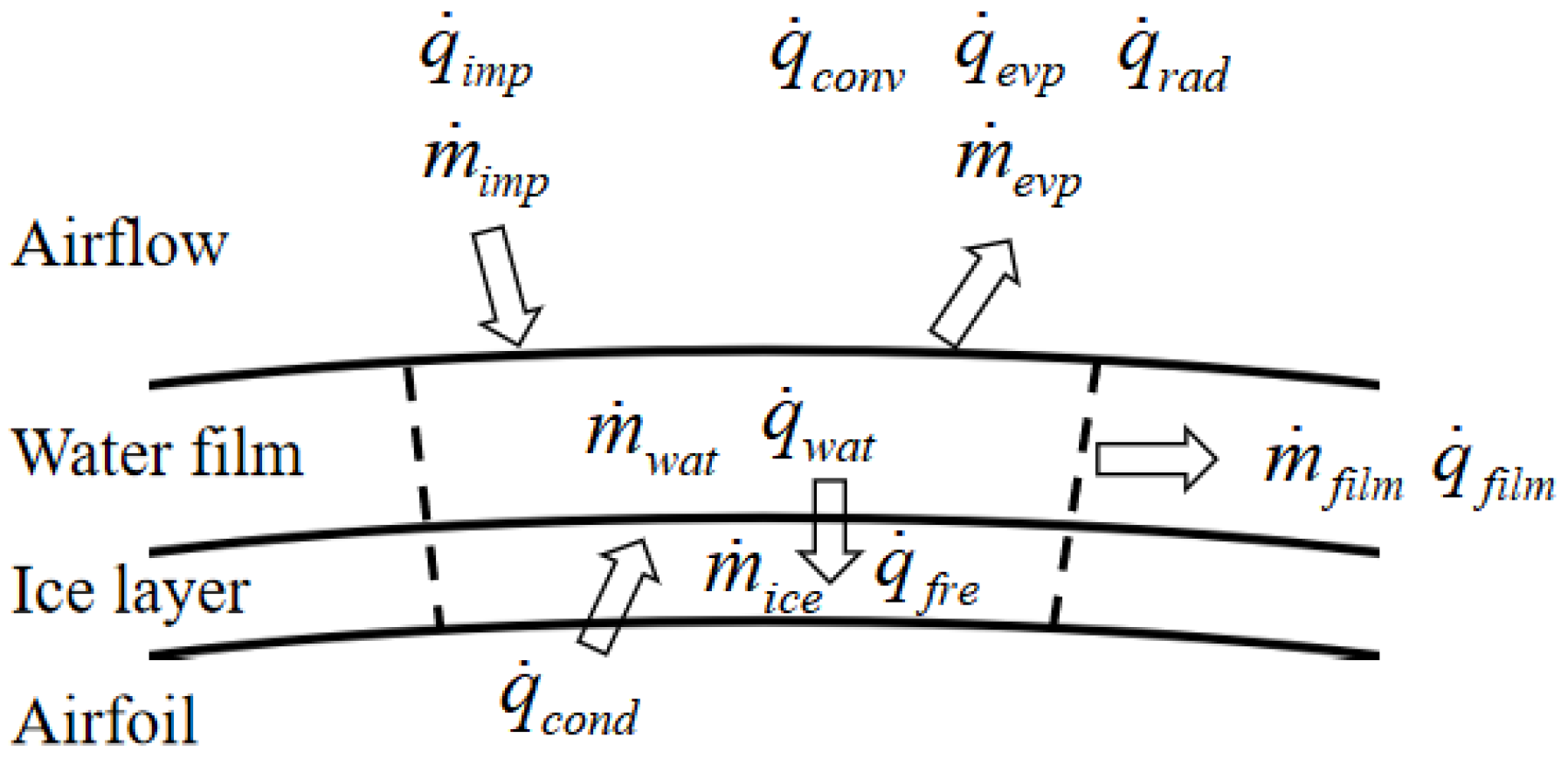
2.1. Governing Equations

In the local thermal protection state, the supercooled droplets will not freeze immediately after hitting the surface but will flow on the surface in the form of water film. In order to simulate the water film flow and icing phenomenon, a numerical simulation method of icing considering water film flow is presented in this paper. The following assumptions need to be made to establish the model: (1) Due to the small thickness and slow speed of the water film, the normal flow of the water film can be ignored, and the water film flow is considered as laminar flow. (2) The physical properties of liquid water, ice, and air do not change during the process of water film flowing and freezing. (3) The water film flows under the action of air shear force, and the two are unidirectionally coupled. (4) The water film flow is not affected by the impact of supercooled droplets. The surface is divided into several control volumes, and the mass and energy conservation equations are established for each control volume.
The water film can be considered Couette flow under the airflow action. The velocity distribution of the water film flow section is considered approximately linear, so the relationship between water film thickness and average water film velocity can be expressed as follows [23,24]:
u ¯ ( s ) = h w 2 μ w τ a ( s ) ,
where h w is the water film thickness, u is the water film velocity at any height, τ a ( s ) is the airflow shear force, and μ w is the dynamic viscosity of liquid water.
As shown in Figure 1, the mass conservation equation of water film in the control volume can be expressed as:
m ˙ w a t + m ˙ f i l m = m ˙ i m p m ˙ e v p m ˙ i c e ,
m ˙ w a t is the change rate of liquid water mass in the control volume:
m ˙ w a t = ( ρ w h w ) t ,
where, ρ w is the water density.
m ˙ f i l m is the mass difference between the inflow and outflow of liquid water in the control volume:
m ˙ f i l m = s 0 h w ρ w u d y ,
m ˙ i m p is the mass of water collected in the control body for supercooled droplet impact. It can be expressed as:
m ˙ i m p = β V L W C ,
where β is the droplet collection coefficient, V is the far-field air velocity, and L W C is the liquid water content.
m ˙ e v p is the mass of evaporation of liquid water under surface heating, which can be expressed as:
m ˙ e v p = h c ρ a R v c p a ( e s u r T w e T ) ,
where h c is the convective heat transfer coefficient, ρ a is the air density, R v is the water vapor gas constant, c p a is specific heat capacity of air, T w is the surface temperature of liquid water, T is the far-field temperature, and e s u r and e are the saturated water vapor pressure of the surface and far-field flow, respectively. Both values can be calculated according to the following formula [25,26]:
e = 611.011 + 44.481 ( T T m ) + 1.419 ( T T m ) 2 + 0.0239 ( T T m ) 3 + 1.744 × 10 4 ( T T m ) 4 , T < T m , e = 609.603 + 49.495 ( T T m ) + 1.739 ( T T m ) 2 + 0.031 ( T T m ) 3 + 2.292 × 10 4 ( T T m ) 4 , T T m
m ˙ i c e is the mass of frozen water.
The energy conservation equation established in the control volume can be expressed as:
q ˙ c o n d + q ˙ i m p = q ˙ c o n v + q ˙ e v p + q ˙ r a d + q ˙ f r e + q ˙ w a t + q ˙ f i l m ,
where q ˙ c o n d is the heating flux received, that is, the heating power of the local thermal protection.
q ˙ i m p is the heat flux caused by the impact of the water droplets:
q ˙ i m p = m ˙ i m p [ c p i T m + L f + c p w ( T T m ) + V d 2 2 ] ,
q ˙ c o n v is the heat flux of the convective heat transfer between the surface of the water film and the airflow:
q ˙ c o n v = h c ( T w T r e c ) ,
q ˙ e v p is the heat flux density of evaporation on the surface of the water film:
q ˙ e v p = m ˙ e v p [ c p i T m + L f + c p w ( T w T m ) + L e ] ,
q ˙ r a d is the radiant heat flux on the water film surface:
q ˙ r a d = σ ( T w 4 T 4 ) ,
q ˙ f r e is the heat flux of frozen liquid water:
q ˙ f r e = m ˙ i c e c p i T w ,
q ˙ w a t is the heat flux of change rate of liquid water mass:
q ˙ w a t = m ˙ w a t [ c p i T m + L f + c p w ( T w T m ) ] ,
q ˙ f i l m is the heat flux of liquid water flow in and out of control volume:
q ˙ f i l m = m ˙ f i l m [ c p i T m + L f + c p w ( T w T m ) ] ,
where c p i is the specific heat capacity of ice, c p w is the specific heat capacity of water, L f is the latent heat of melting of ice, L e is the latent heat of evaporation of water, T m is the phase transition equilibrium temperature, and T r e c is the boundary layer recovery temperature.

2.2. Solution Method

There are three unknown parameters ( T w , h w , m ˙ i c e ) in the conservation equations of mass and energy, so a governing equation needs to be added. The Stefan boundary condition applied to ice-water interface is [27,28]:
m ˙ i c e L f = k w T w y + k i T i y ,
When the anti-icing process is not considered, the heat flow on the surface is considered 0. If, at this time, the internal temperature of the ice layer is the same, and the temperature changes can be ignored, then:
m ˙ i c e L f = k w ( T m T w ) / h w ,
where, k w is the thermal conductivity of water, and k i is the thermal conductivity of ice.
In the solution process, the water film thickness is assumed first. The water film surface temperature and icing rate are solved by the Equations (12) and (20). Then, the surface water film thickness is obtained by solving Equation (6) using the surface temperature and icing rate. The icing rate can be obtained by iterative solutions until the water film thickness is stable.

2.3. Calculation of Convective Heat Transfer Coefficient

The calculation method of the convective heat transfer coefficient on the icing surface mainly adopts the boundary layer integration method, and the influence of roughness on flow is taken into account in the calculation process.
The whole region is divided into laminar flow and turbulent flow, and local roughness Reynolds number is used as the discrimination method, which is defined as:
Re k = V k k s / ν a ,
where ν a is the kinematic viscosity of air, V k is the airflow velocity at the roughness height, and k s is the surface roughness height. The equivalent gravel roughness is usually used for icing roughness [29]. In this paper, the icing model considering water film flow is studied. For the water film flow region, the surface roughness can be considered as the wave height of the water film flow [30,31], which expressed as:
k s = 0.75 τ a μ w h w 3 g ,
The local rough Reynolds numbers at different positions are calculated, and then judged according to the critical Reynolds number. The judgment criteria are as follows:
Re c = { 10 22 3834.2 198460 | s | + 3281200 | s | 2 6999400 600 | s | 3 | s | = 0 | s | < 0.035 c , | s | 0.035 c
where s is the surface distance from the control volume to the stagnation point, and c is the chord length. When Re k < Re c , the flow is considered as laminar flow and when Re k Re c , the flow is considered as turbulent flow.
The calculation of the convective heat transfer coefficient is usually described by Stanton number, and the convective heat transfer coefficient can be expressed as:
h c = S t ρ a V e c p a ,
For the laminar flow region, its Stanton number can be expressed as:
S t l = 0.418 ν a 0.5 V e 0.435 ( 0 s V e 1.87 d s ) 0.5 ,
Therefore, the convective heat transfer coefficient in the laminar region can be expressed as:
h c l = 0.296 λ a ν a ( V e 2.88 0 s V e 1.88 d s ) 0.5 ,
where λ a is the thermal conductivity of air and V e is the velocity at the outer edge of boundary layer.
For the turbulent region, its Stanton number can be expressed as:
S t t = c f / 2 Pr t + c f / 2 / S t k ,
where Pr t is the Prandtl number in the turbulent region, which can be approximately taken as 0.9. S t k is the Stanton number of roughness surface, which can be expressed as:
S t k = 0.936 ( 0.0125 Re δ 2 1 / 4 V e 2 ) 1 / 2 k s ν a ,
c f is the friction coefficient under turbulence state, which can be expressed as:
c f 2 = [ 0.41 ln ( 864 δ 2 , t / k s + 2.568 ) ] 2 ,
where δ 2 , t is the momentum thickness of the turbulent flow. Considering that the development of turbulence flow is based on the development of laminar flow, the momentum thickness of turbulent flow is considered from the transition point based on the momentum thickness of laminar flow. The momentum thickness in the laminar flow region and the turbulent region can be expressed as:
δ 2 , l = 0.664 ν a 0.5 V e 2 . 84 ( 0 s t r V e 4 . 68 d s ) 0.5 ,
δ 2 , t = 0.0156 υ a 0.5 V e 4.11 ( S t r S 2 V e 3.86 d s ) 4 / 5 + δ 2 , t r ( V e , t r V e ) 3.288 ,
Therefore, the convective heat transfer coefficient in the turbulent region can be expressed as:
h t ( s ) = S t ρ V e c p = [ c f / 2 Pr t + c f / 2 ( 1 / S t k ) ] ρ V e c p ,
In solving, first, the surface stagnation point is found. Then, the distance between each control volume and stagnation point is calculated, and the local roughness Reynolds number is used to judge the flow state. Finally, the calculation method of the laminar or turbulent convective heat transfer coefficient is selected for icing calculation.

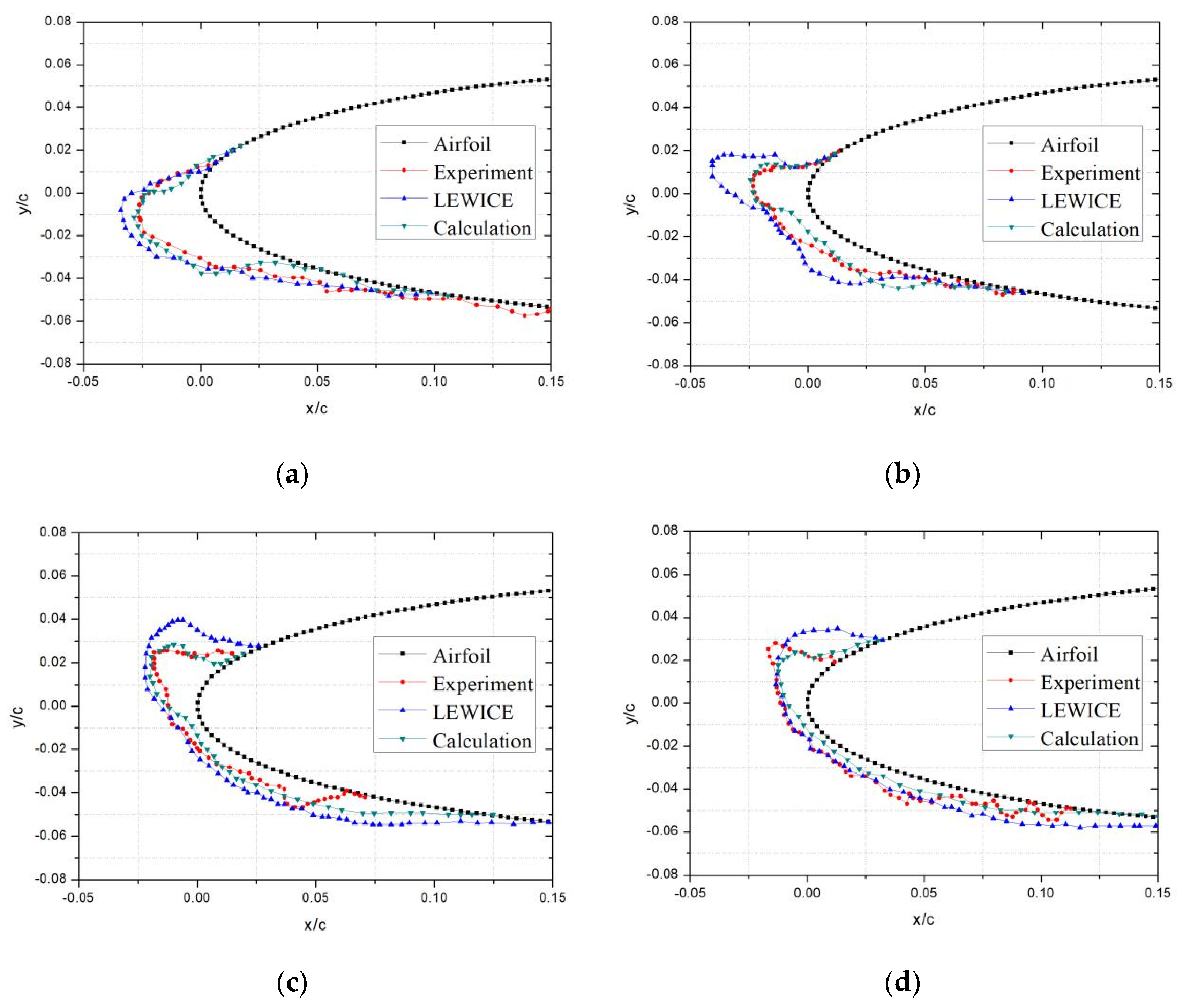
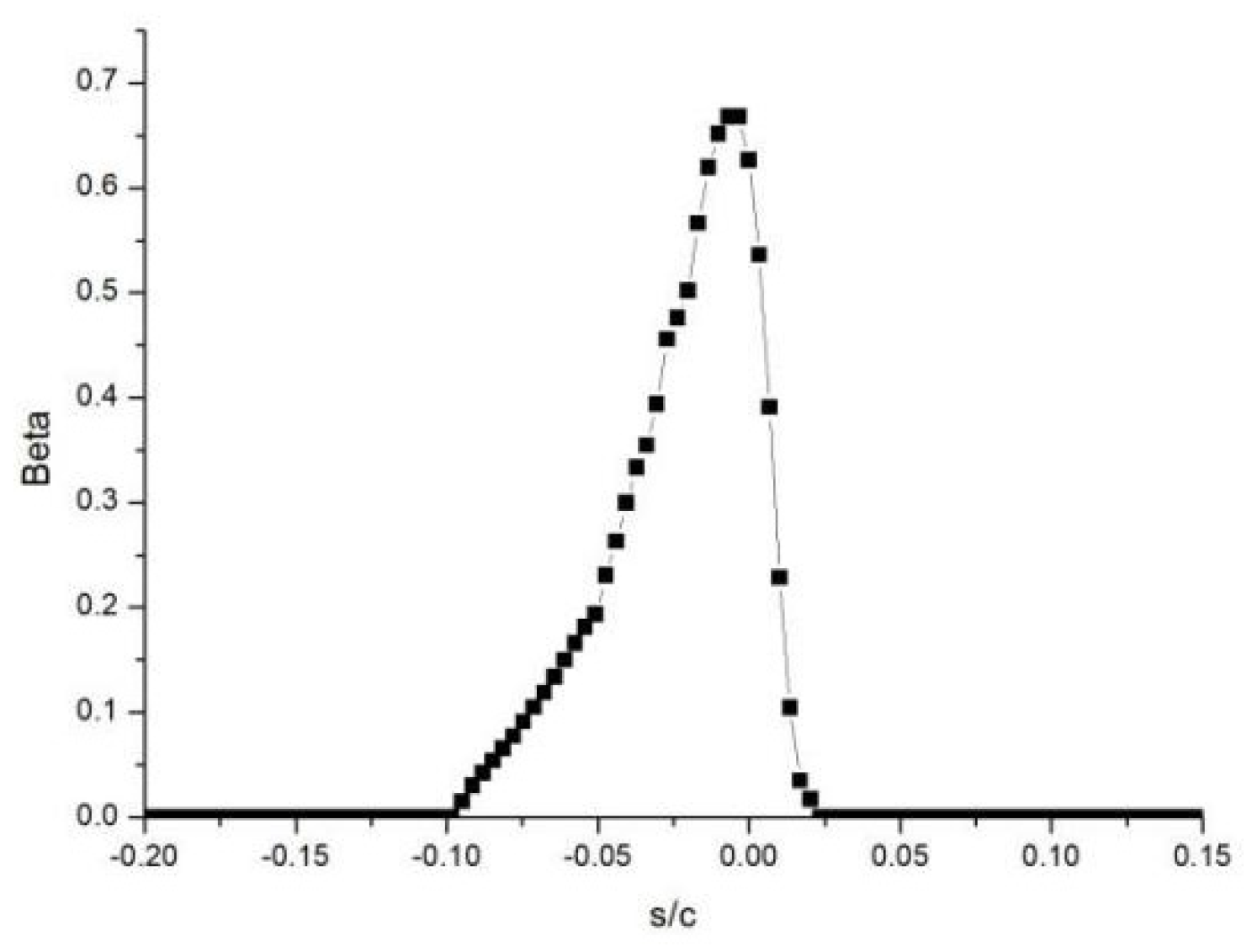
3. Method Validation

In order to verify the effectiveness of the method, the icing experiment conditions are selected for numerical simulation, and the calculation results are compared with the experimental data and the LEWICE calculation [25,30,32]. The icing calculation based on the Messinger model was adopted in the LEWICE [33,34]. The NACA0012 airfoil was selected as the geometry model, and the chord length was 0.5334 m. The calculation conditions are shown in Table 1. The calculation process included grid generation, flow field calculation, droplet trajectory calculation, and icing shape calculation. The same grid, airflow, and droplet impact characteristics results were used in the calculation, and the icing model adopted the method described above.
The calculation results are shown in Figure 2. Case 1 is a typical rime ice condition. From Figure 2a, it can be seen that the numerical simulation results are not different from the experimental results and LEWICE results and have good simulation accuracy. This is because, under the rime ice condition, supercooled droplets form ice immediately after hitting the surface, and there is no liquid water flowing on the surface. At this time, the icing equations of mass and energy can be simplified.
Case 4 is a typical glaze ice condition. It can be seen from Figure 2d that the results of the icing model based on water film flow are closer to the experimental data than the LEWICE results, especially at the upper corner of the ice shapes. This indicates that the model presented in this paper can have better simulation accuracy under glaze ice condition. This is because the icing temperature of rime ice is relatively high, and supercooled droplets cannot be frozen immediately after hitting the surface. Instead, a large part of supercooled droplets flow on the surface in the form of liquid water and freeze gradually. The icing model based on water film flow better describes the physical process of liquid water flowing on the surface. In contrast, the LEWICE simulation accuracy is relatively low, resulting in the deviation of ice shape.
The icing conditions of cases 2 and 3 are similar to case 4. The icing conditions should be mixed, and the ice shapes are like horns. Under these conditions, the icing model based on water film flow can be closer to the experimental results.
As can be seen from the comparison results under different cases in Figure 1, the icing model presented in this paper can simulate icing under different conditions, and the calculation results are closer to the experimental values.

4. Numerical Simulation of Icing under Local Thermal Protection State

In the unprotected state, it can be considered that the heat flux input by the anti-icing system through the surface is 0, while under the local thermal protection state, the surface heat flux is given according to the set value of the anti-icing system. Case 3 in Table 1 is used as a calculation model and icing condition. The distribution of the droplet collection coefficient is shown in Figure 3. The distribution range of the droplet collection coefficient is within s/c = ±0.1. Based on this, different protection ranges were designed, and the influence of different protection power on ice shapes was analyzed.

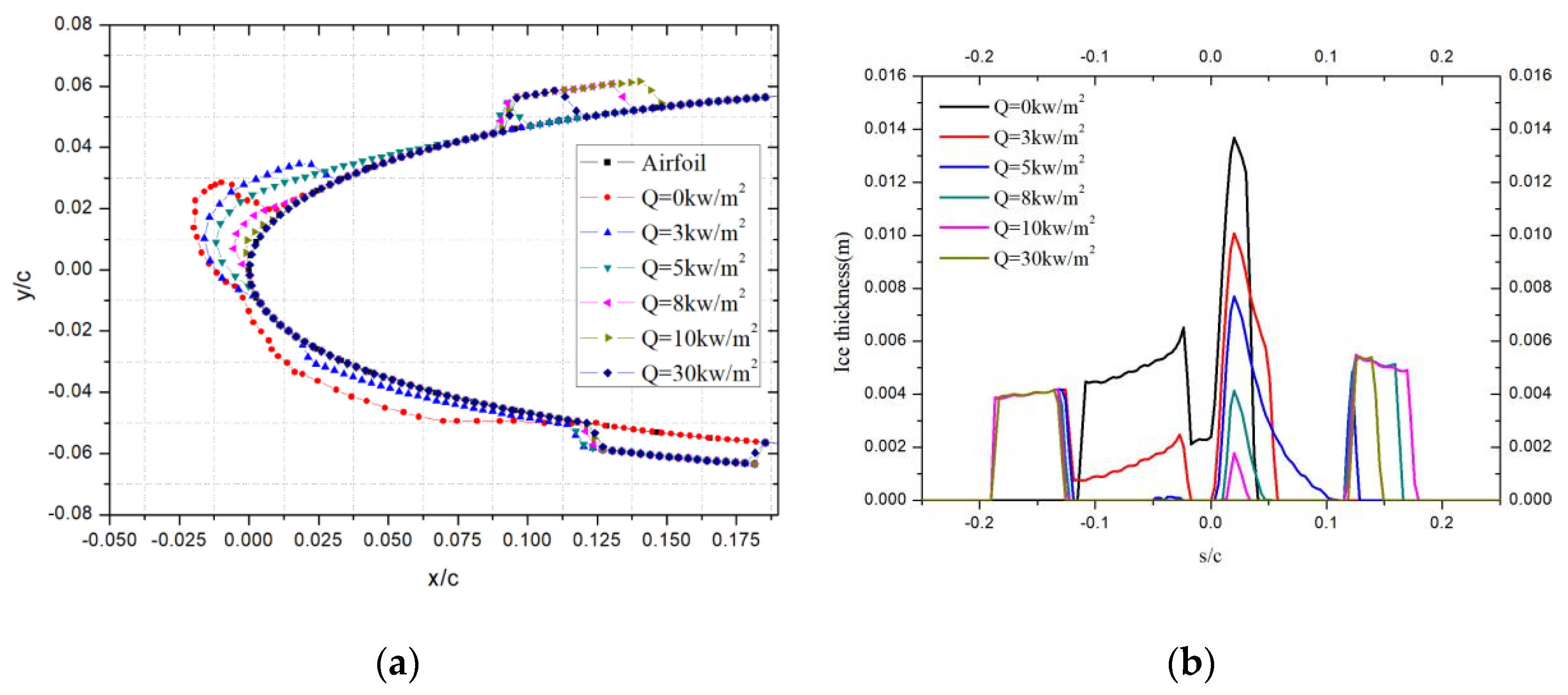
4.1. Protection Range Is s/c = ±0.2

The thermal protection area was set as s/c = ±0.2. Various heating powers such as 0kw/m2 (that is not anti-icing), 3 kw/m2, 5 kw/m2, 8 kw/m2, 10 kw/m2, and 30 kw/m2 were selected in the calculation, and the calculation results are shown in Figure 4.
When the heating power was 3 kw/m2, there was no ice near the stagnation point at the leading edge, but there was still icing on the upper and lower sides. This is because the heating at the leading edge prevents the impacted supercooled droplets from freezing but does not completely evaporate the droplets. Droplets flow to the upper and lower sides in the form of liquid water under the action of airflow. The anti-icing heat load required on the upper and lower sides is relatively large, but the heating power is insufficient to ensure that the liquid water does not freeze; therefore, icing is formed on both sides. When the heating power reached 5 kw/m2, the ice amount on the upper side was significantly reduced, and the icing range was expanded in Figure 4b. Compared with 3 kw/m2, the increase of heating power led to an increase in the temperature of liquid water, and the liquid water needed to flow over a longer distance to freeze; therefore, although the icing amount decreased, the icing range increased. Due to the higher heating power, there is no ice accretion on the lower side. As the power gradually increases further, it can be seen that the icing on the surface gradually decreases. When the heating power reaches 10 kw/m2, there is almost no icing on the surface.

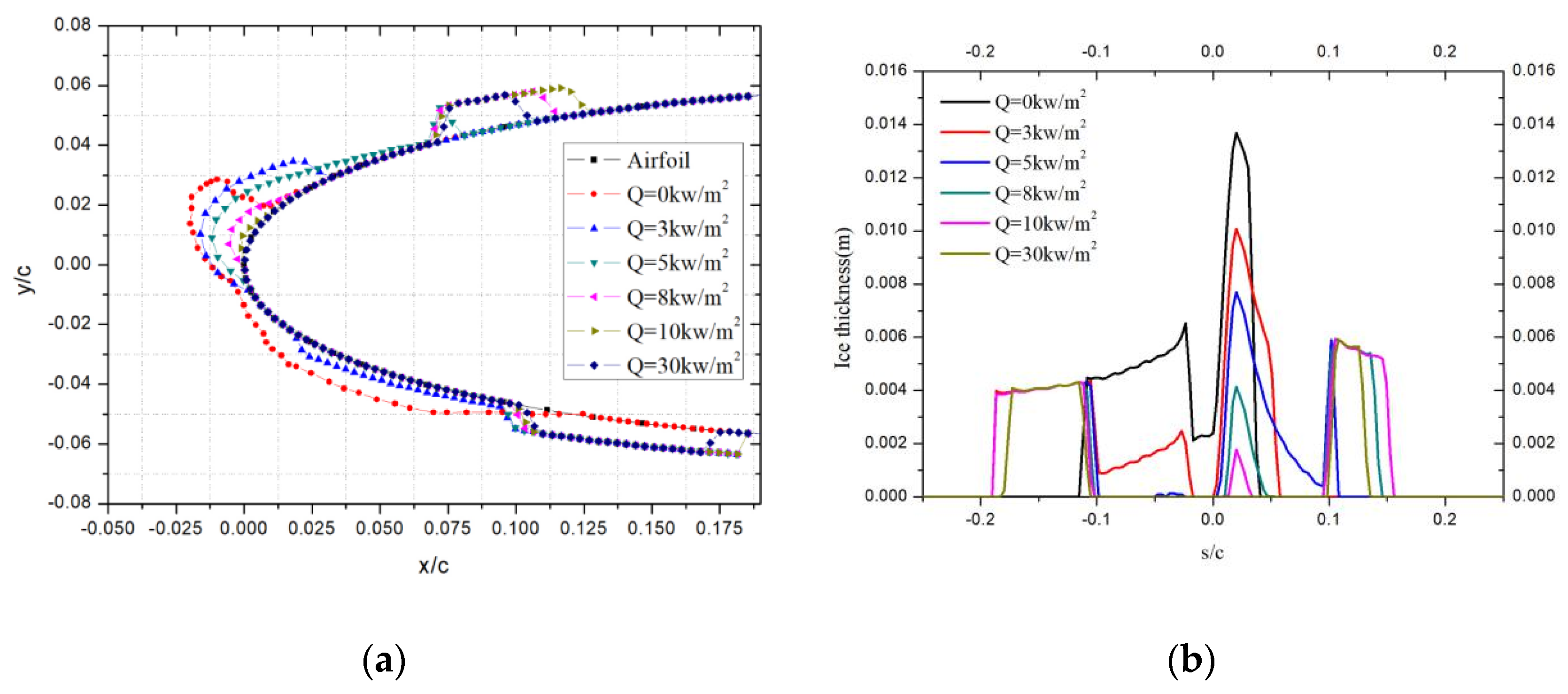
4.2. Protection Range Is s/c = ±0.12

The thermal protection area was set as s/c = ±0.12, and various heating powers were used in the calculation. The calculation results are shown in Figure 5. When the thermal protection area becomes smaller, ice ridges are formed outside the upper and lower protection ranges. Taking the heating power of 30kw/m2 as an example, when the protection range is s/c = ±0.2, there is no ice formation on the surface, but when the protection range is s/c = ±0.12, ice ridges occur outside the protection area on the upper and lower surfaces in Figure 5b. This is because the protection range is reduced so that the liquid water cannot evaporate completely but flows out of the protection area under the action of airflow and freezes into ice ridges. The same phenomenon occurs when the heating power is 10 kw/m2, and the range of ice ridge increases gradually. As the heating power further decreases, it can be found that the ice amount on the leading edge gradually increases, but the amount of ice ridge at the rear gradually decreases. When the power was 3kw/m2, icing occurred at the leading edge, and there was almost no ice ridge formation. This phenomenon occurs because when the heating power is large, there is more evaporation of liquid water, so there is less water flowing out of the protected area, and the amount of ice ridge decreases. When the heating power is low, liquid water freezes at the leading edge, so there is less liquid water flowing out of the surface and fewer ice ridges. Therefore, there is a critical heating power. Under this power state, ice will not be formed in large amounts at the leading edge due to heating, and the impacted droplets will flow in the form of liquid water. On the other hand, because the heating power is not high, it is difficult for the liquid water to evaporate completely, resulting in more liquid water flowing out of the protection area and forming ice ridges, which affects the aerodynamic characteristics. This example shows that when the anti-icing system works, if the heating power of anti-icing is not high enough and only local thermal protection is provided, ice ridges may be formed outside the protection range. This kind of incomplete thermal protection not only cannot play the role of icing protection but also may cause more serious hazards to flight safety.

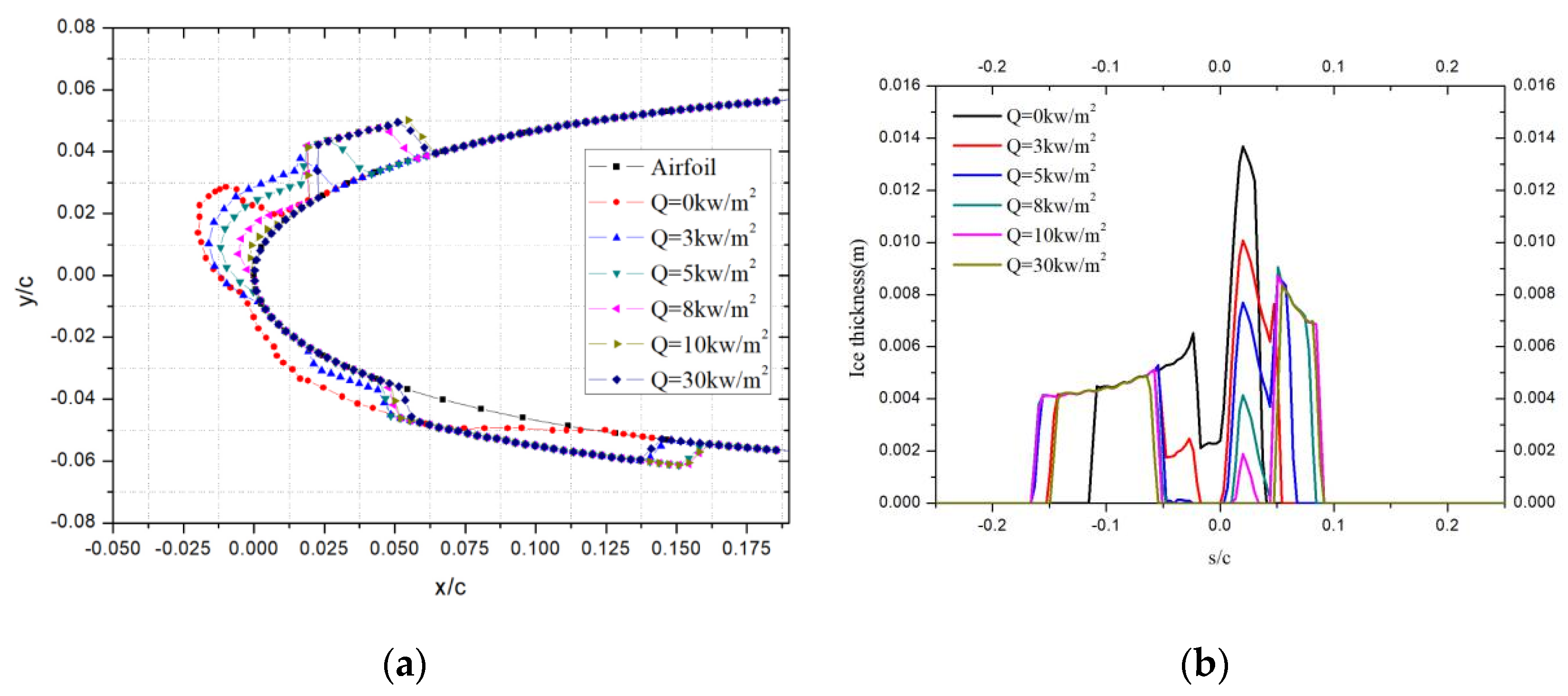
4.3. Protection Range Is s/c = ±0.1

As shown in Figure 6, when the protection range was set to s/c = ±0.1, the calculated ice shapes were similar to that of s/c = ±0.12, but the position of the ice ridge formation was more forward. When the heating power is 5 kw/m2, icing is formed on the upper side. When the liquid water flows out of the protection area, it freezes and forms a sharp ice ridge in Figure 6a.

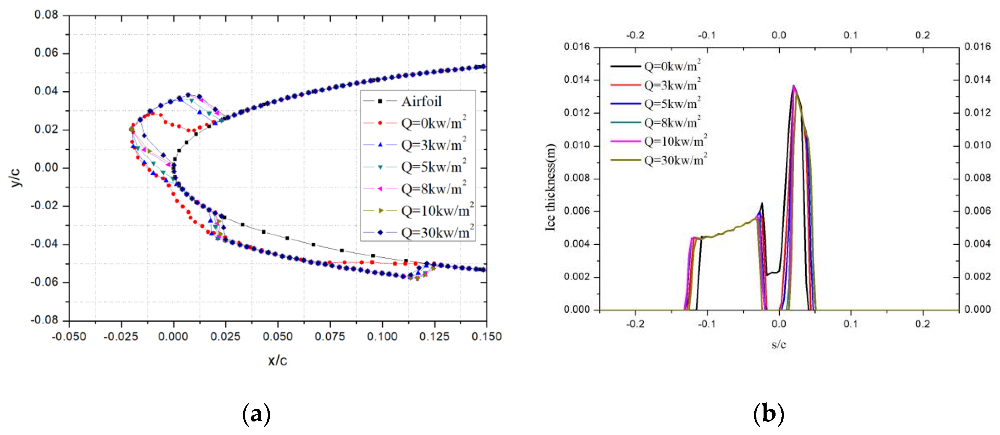
4.4. Protection Range Is s/c = ±0.05

When the protected range was further reduced to s/c = ±0.05, as shown in Figure 7, it can be found that the icing area affected by local heating at the leading edge gradually decreased. The ice ridge gradually fused with the ice at the leading edge area, resulting in more ice accumulation occurring at the position separated from the protection area.

4.5. Protection Range Is s/c =±0.02

When the protection range was s/c = ±0.02, the calculation results are shown in Figure 8. There was no icing in the protection area, but there was larger ice accumulation outside the protection area, forming a shape like a sheep’s horn. At the same time, with the increase of heating power, the ice formation position on the upper and lower sides gradually retreats, as seen in Figure 8b. This is because the higher the heating power, the higher the temperature of liquid water, so the icing position is relatively backward.

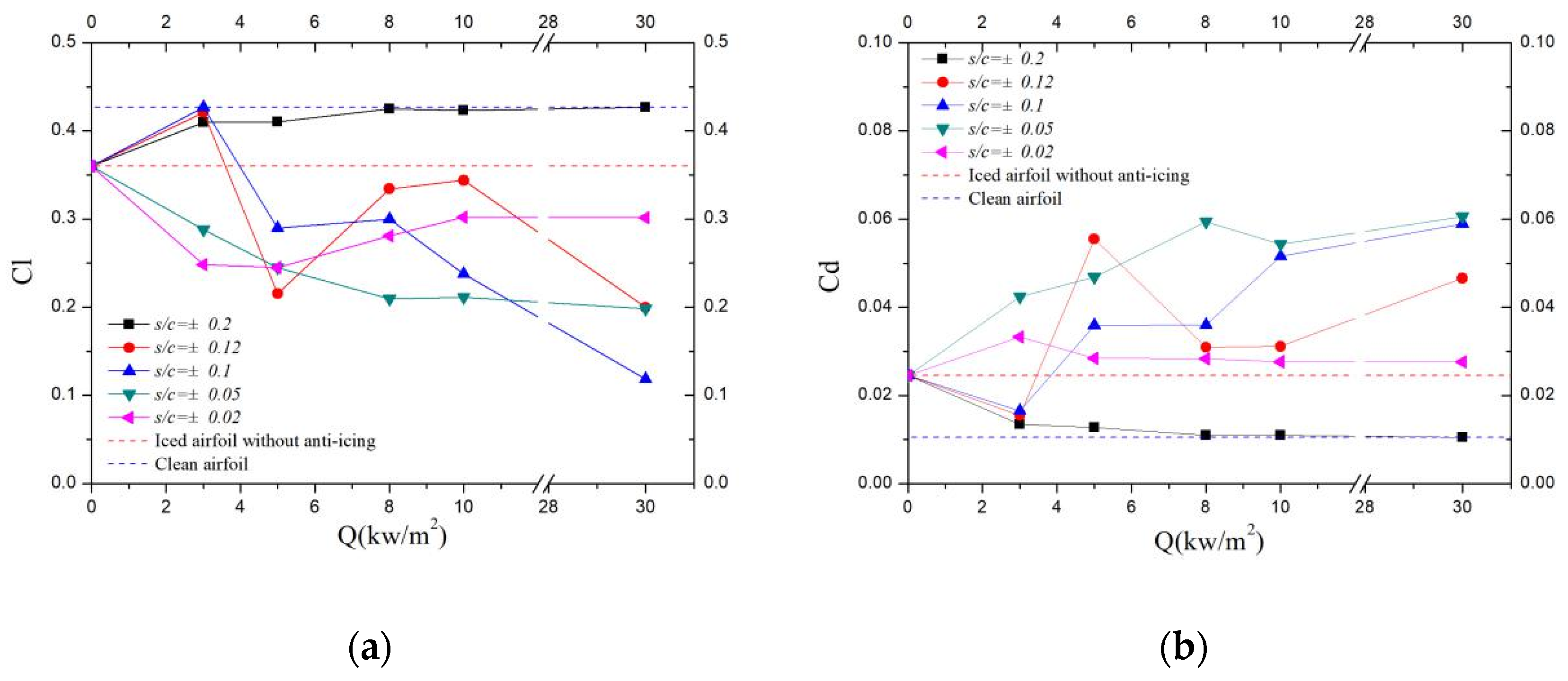
4.6. Aerodynamic Characteristic Analysis

According to the ice shapes in Figure 4, Figure 5, Figure 6, Figure 7 and Figure 8, the aerodynamic coefficient of the airfoil after icing under local thermal protection states are calculated, as shown in Figure 9. When the protection range is s/c = ±0.2, regardless of the protection power, local thermal protection can increase the lift coefficient and decrease the drag coefficient of the airfoil compared with the unprotected state. When the protection range is less than s/c = ±0.12, local thermal protection may lead to a decrease in lift coefficient and an increase in drag coefficient. Taking the protection range s/c = ±0.1 as an example, the lift coefficient decreases gradually with the increase of heating power. This is because the liquid water forms ice ridges outside the protection area, which leads to the deterioration of the aerodynamic characteristics. Taking the protection power of 10kw/m2 as an example, the lift coefficient does not increase with the increase of the protection range. Therefore, with the expansion of the thermal protection range, the icing on the airfoil surface gradually moves backward, leading to the formation of ice ridges outside the protected area.
The flow field of the airfoil before and after icing are shown in Figure 10. It can be seen that the streamlines of the clean airfoil are smooth, and the aerodynamic characteristics are the best. Figure 10b shows the flow field of an iced airfoil in the unprotected state. The icing destroys the original streamline and forms a vortex behind the ice shape. In the state shown in Figure 10c, ice ridges are formed on the airfoil. The obstruction of ice ridges results in a negative pressure area, but since the ice ridges are small, the damage to the aerodynamic properties is limited. However, in Figure 10d, the larger ice ridge leads to a large range of vortices behind the ice ridge, and the aerodynamic characteristics are worse than those in the unprotected state. Therefore, ice ridges are more dangerous than icing.
These results indicate that the increase of total protection energy consumption may make the aerodynamic characteristics of the airfoil after icing worse. Therefore, reasonable protection range and protection power need to be considered in the design of anti-icing systems to prevent the hazards of ice ridges.

5. Conclusions

Numerical simulation of icing under local thermal protection state was studied in this paper. An icing model based on water film flow was presented, the modeling ideas, governing equations, and solution methods were displayed, and the calculation method of convective heat transfer coefficient was given. Finally, the icing model based on water film flow used to calculate icing under different protection ranges and protection powers, and the results were analyzed. The following conclusions were drawn:
(1)
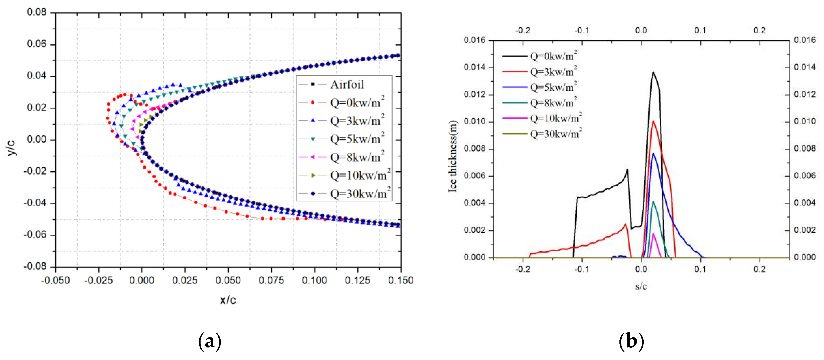
When the local thermal protection power is high, there is no ice formation in the protection area, but ice ridges may be formed outside the icing protection area. When the local thermal protection power is low, the ice amount in the protection area will decrease, but the icing will still occur. With the expansion of the protection range, the position of the ice ridge will gradually move backward;
(2)
When the combination of protection range and protection power is inappropriate, there is less ice at the leading edge of the airfoil, but many ice ridges will be accumulated outside the protection area;
(3)
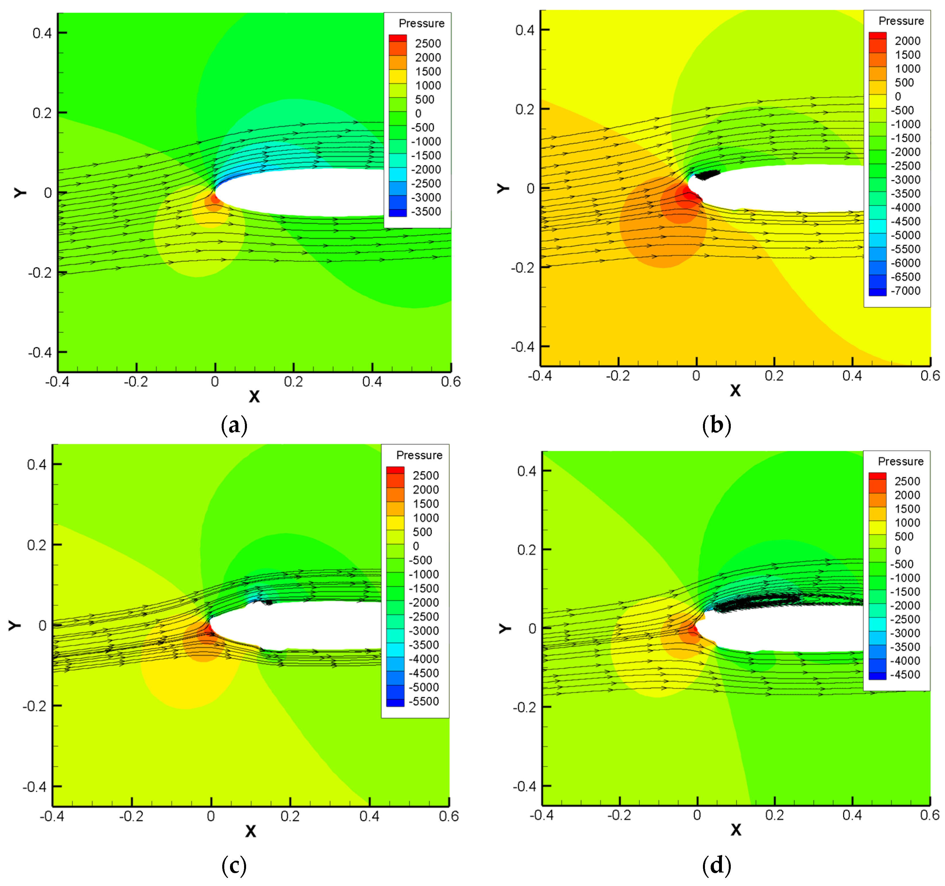
The formation of ice ridges can lead to negative pressure areas and vortices on the airfoil surface, resulting in the deterioration of aerodynamic characteristics, which is more dangerous than icing;
(4)
In the design of thermal anti-icing systems, it is necessary to select reasonable heating power and protection range; otherwise, more dangerous ice ridges may be formed, which will fail to achieve protection effect and increase the risk of aircraft.

Author Contributions

Conceptualization, Z.W. and S.L.; methodology, H.Z.; software, Z.W.; validation, Z.W., H.Z. and S.L.; writing—original draft preparation, Z.W.; writing—review and editing, Z.W. and S.L.; funding acquisition, Z.W., H.Z. and S.L. All authors have read and agreed to the published version of the manuscript.

Funding

This research was funded by the National Natural Science Foundation of China (Grant No.51806105), the Open Fund of the Key Laboratory of Icing and Anti/De-icing (Grant No. IADL20190309) and the Scientific Research Foundation of Nanjing Institute of Technology (Grants No. YKJ202009).

Institutional Review Board Statement

Not applicable.

Informed Consent Statement

Not applicable.

Data Availability Statement

The data presented in this study are available on request from the corresponding author.

Conflicts of Interest

The authors declare no conflict of interest.

References

  1. Pourbagian, M.; Habashi, W.G. Aero-thermal optimization of in-flight electro-thermal ice protection systems in transient de-icing mode. Int. J. Heat Fluid Flow 2015, 54, 167–182. [Google Scholar] [CrossRef]
  2. Dong, W.; Zhu, J.; Zheng, M.; Chen, Y. Thermal analysis and testing of nonrotating cone with hot-air anti-icing system. J. Propuls. Power 2015, 31, 896–903. [Google Scholar] [CrossRef]
  3. Pourbagian, M.; Talgorn, B.; Habashi, W.G.; Kokkolaras, M.; Le Digabel, S. Constrained problem formulations for power optimization of aircraft electro-thermal anti-icing systems. Optim. Eng. 2015, 16, 663–693. [Google Scholar] [CrossRef]
  4. Lynch, F.T.; Khodadoust, A. Effects of ice accretions on aircraft aerodynamics. Prog. Aerosp. Sci. 2001, 37, 669–767. [Google Scholar] [CrossRef]
  5. Farzad, M.; Fortin, G.; Dolatabadi, A. Quantitative analysis of rivulet/ice formation on a heated airfoil by Color-Coded Point Projection method. Cold Reg. Sci. Technol. 2021, 188, 103298. [Google Scholar] [CrossRef]
  6. Al-Khalil, K.M.; Keith, T.G., Jr.; De Witt, K.J. Development of an improved model for runback water on aircraft surfaces. J. Aircr. 1994, 31, 271–278. [Google Scholar] [CrossRef]
  7. Morency, F.; Tezok, F.; Paraschivoiu, I. Anti-icing system simulation using CANICE. J. Aircr. 1999, 36, 999–1006. [Google Scholar] [CrossRef]
  8. Morency, F.; Tezok, F.; Paraschivoiu, I. Heat and mass transfer in the case of anti-icing system simulation. J. Aircr. 2000, 37, 245–252. [Google Scholar] [CrossRef]
  9. Silva, G.; Silvares, O.; Zerbini, E. Airfoil anti-ice system modeling and simulation. In Proceedings of the 41st Aerospace Sciences Meeting and Exhibit, Reno, NV, USA, 6–9 January 2003. [Google Scholar]
  10. Silva, G.; Silvares, O.; Zerbini, E. Numerical simulation of airfoil thermal anti-ice operation, part 1: Mathematical modelling. J. Aircr. 2007, 44, 627–633. [Google Scholar] [CrossRef]
  11. Miller, D.; Addy, H.; Ide, R. A study of large droplet ice accretions in the NASA-Lewis IRT at near-freezing conditions. In Proceedings of the 34th Aerospace Sciences Meeting and Exhibit, Reno, NV, USA, 15–18 January 1996. [Google Scholar]
  12. Lee, S.; Dunn, T.; Gurbacki, H.; Bragg, M.; Loth, E. An experimental and computational investigation of spanwise-step-ice shapes on airfoil aerodynamics. In Proceedings of the 36th AIAA Aerospace Sciences Meeting and Exhibit, Reno, NV, USA, 12–15 January 1998. [Google Scholar]
  13. Lee, S.; Bragg, M. Effects of simulated-spanwise-ice shapes on airfoils-Experimental investigation. In Proceedings of the 37th AIAA Aerospace Sciences Meeting and Exhibit, Reno, NV, USA, 11–14 January 1999. [Google Scholar]
  14. Lee, S.; Bragg, M. Experimental investigation of simulated large-droplet ice shapes on airfoil aerodynamics. J. Aircr. 1999, 36, 844–850. [Google Scholar] [CrossRef]
  15. Lee, S.; Bragg, M. The effect of ridge-ice location and the role of airfoil geometry. In Proceedings of the 19th AIAA Applied Aerodynamics Conference, Anaheim, CA, USA, 11–14 June 2001. [Google Scholar]
  16. Broeren, A.; Whalen, E.; Busch, G.; Bragg, M. Aerodynamic simulation of runback ice accretion. J. Aircr. 2010, 47, 924–939. [Google Scholar] [CrossRef] [Green Version]
  17. Bragg, M.; Broeren, A.; Addy, H.; Potapczuk, M.; Guffond, D.; Montreuil, E. Airfoil ice-accretion aerodynamic simulation. In Proceedings of the 45th AIAA Aerospace Sciences Meeting and Exhibit, Reno, NV, USA, 8–11 January 2007. [Google Scholar]
  18. Broeren, A.; Bragg, M.; Addy, H. Effect of High-Fidelity Ice Accretion Simulations on the Performance of a Full-Scale Airfoil Model. In Proceedings of the 46th AIAA Aerospace Sciences Meeting and Exhibit, Reno, NV, USA, 7–10 January 2008. [Google Scholar]
  19. Uranai, S.; Fukudome, K.; Mamori, H.; Fukushima, N.; Yamamoto, M. Numerical Simulation of the Anti-Icing Performance of Electric Heaters for Icing on the NACA 0012 Airfoil. Aerospace 2020, 7, 123. [Google Scholar] [CrossRef]
  20. Fukudome, K.; Tomita, Y.; Uranai, S.; Mamori, H.; Yamamoto, M. Evaluation of Anti-Icing Performance for an NACA0012 Airfoil with an Asymmetric Heating Surface. Aerospace 2021, 8, 294. [Google Scholar] [CrossRef]
  21. Wang, Z.; Zhu, C. Numerical simulation of three-dimensional rotor icing in hovering flight. Proc. Inst. Mech. Eng. Part G J. Aerosp. Eng. 2018, 232, 545–555. [Google Scholar] [CrossRef]
  22. Zhu, C.; Zhu, C.; Guo, T. Multi-Zone ice accretion and roughness models for aircraft icing numerical simulation. Adv. Appl. Math. Mech. 2016, 8, 737–756. [Google Scholar] [CrossRef]
  23. Bourgault, Y.; Beaugendre, H.; Habashi, W. Development of a shallow-water icing model in FENSAP-ICE. J. Aircr. 2000, 37, 640–646. [Google Scholar] [CrossRef]
  24. Karev, A.; Farzaneh, M.; Lozowski, E. Character and stability of a wind-driven supercooled water film on an icing surface—II. Transition and turbulent heat transfer. Int. J. Therm. Sci. 2003, 42, 499–511. [Google Scholar] [CrossRef]
  25. Dai, H.; Zhu, C.; Zhao, H.; Liu, S. A New Ice Accretion Model for Aircraft Icing Based on Phase-Field Method. Appl. Sci. 2021, 11, 5693. [Google Scholar] [CrossRef]
  26. Huang, J.R.; Keith, T.G., Jr.; De Witt, K.J. Efficient Finite Element Method for Aircraft De-Icing Problems. J. Aircr. 1993, 30, 695–704. [Google Scholar] [CrossRef]
  27. Myers, T.G. Extension to the Messinger model for aircraft icing. AIAA J. 2001, 39, 211–218. [Google Scholar] [CrossRef] [Green Version]
  28. Zhang, X.; Min, J.; Wu, X. Model for aircraft icing with consideration of property-variable rime ice. Int. J. Heat Mass Transf. 2016, 97, 185–190. [Google Scholar] [CrossRef]
  29. Shin, J.; Bond, T.H. Experimental and Computational Ice Shapes and Resulting Drag Increase for a NACA 0012 Airfoil; NASA Technical Manual 105743; NASA Office of the Chief Information Officer: Hampton, VA, USA, 1992.
  30. Fortin, G.; Laforte, J.L.; Ilinca, A. Heat and mass transfer during ice accretion on aircraft wings with an improved roughness model. Int. J. Therm. Sci. 2006, 45, 595–606. [Google Scholar] [CrossRef]
  31. Fortin, G.; Ilinca, A.; Laforte, J.L.; Brandi, V. New roughness computation method and geometric accretion model for airfoil icing. J. Aircr. 2004, 41, 119–127. [Google Scholar] [CrossRef] [Green Version]
  32. Han, Y.; Palacios, J. Airfoil-performance-degradation prediction based on nondimensional icing parameters. AIAA J. 2013, 51, 2570–2581. [Google Scholar] [CrossRef]
  33. Wright, W.B. User’s Manual for LEWICE Version 3.2; NASA Technical Manual 214255; NASA Office of the Chief Information Officer: Hampton, VA, USA, 2008.
  34. Ruff, G.A.; Berkowitz, B.M. Users Manual for The NASA Lewis Ice Accretion Prediction Code(LEWICE); NASA Technical Manual 185129; NASA Office of the Chief Information Officer: Hampton, VA, USA, 1990.
Figure 1. Diagram of mass and heat transfer of control volume.
Aerospace 09 00084 g001
Figure 2. Comparison of ice shapes under different conditions: (a) Case 1; (b) Case 2; (c) Case 3; (d) Case 4.
Aerospace 09 00084 g002
Figure 3. Distribution of droplet collection coefficient.
Aerospace 09 00084 g003
Figure 4. Icing characteristics with protection range of s/c = ±0.2: (a) Ice shapes; (b) Ice thickness.
Aerospace 09 00084 g004
Figure 5. Icing characteristics with protection range of s/c = ±0.12: (a) Ice shapes; (b) Ice thickness.
Aerospace 09 00084 g005
Figure 6. Icing characteristics with protection range of s/c = ±0.1: (a) Ice shapes; (b) Ice thickness.
Aerospace 09 00084 g006
Figure 7. Icing characteristics with protection range of s/c = ±0.05: (a) Ice shapes; (b) Ice thickness.
Aerospace 09 00084 g007
Figure 8. Icing characteristics with protection range of s/c = ±0.02: (a) Ice shapes; (b) Ice thickness.
Aerospace 09 00084 g008
Figure 9. Aerodynamic characteristics of airfoil after icing: (a) Cl; (b) Cd.
Aerospace 09 00084 g009
Figure 10. Streamline and pressure distribution of airfoil: (a) Clean airfoil; (b)Iced airfoil without ant-icing; (c) Iced airfoil with protection range of s/c = ±0.12 and protection power of 8 kw/m2; (d) Iced airfoil with protection range of s/c = ±0.05 and protection power of 8 kw/m2.
Aerospace 09 00084 g010
Table 1. Icing calculation conditions.
CaseMaAngle of attack
°
Pressure
Pa
Temperature KMVD
μm
LWC
g·m3
Icing Time
s
10.1974.0101,300244.8020.01.0360
20.1974.0101,300263.1420.01.0360
30.1974.0101,300267.0220.01.0360
40.1974.0101,300268.6920.01.0360
Publisher’s Note: MDPI stays neutral with regard to jurisdictional claims in published maps and institutional affiliations.

