1. Introduction
In recent years, unmanned aerial vehicles (UAVs) have been widely used in mapping, photography, search and rescue, strike, reconnaissance, and mountain, urban, highway, and oil/gas inspections. As part of path planning, coverage path planning (CPP) [
1,
2,
3] of UAV is also very important in mapping, searching, and patrol inspection [
4,
5,
6,
7]. Among commonly used UAVs, rotor UAVs are flexible, can hover and vertically lift, and have low requirements on the take-off site, but at the same time, suffer from small load, low cruise speed, and short endurance time. On the other hand, fixed-wing UAVs are less flexible than rotorcraft, but they have heavy load, fast cruise speed, and long endurance. Therefore, the use of rotorcraft has advantages in missions featuring small areas, large terrain fluctuations, fixed-point lighting, fixed-point shouting, and short-range high-precision tracking shooting, whereas for large-area and long-distance area coverage, patrol inspection, mapping, and search, fixed-wing UAVs are obviously more suitable.
Fixed-wing UAVs in area CPP applications usually plan a scan-type path (a group of parallel lines covering a certain area that are executed in turns, and no crossing of lines is allowed) based on the actual need. While such demand can be met most of the time, in some special applications such as digital orthophoto map (DOM) generation and tilt photography model generation, the lateral distance between two adjacent planned paths is usually less than the UAV’s turning radius. This increases the distance traveled by the fixed-wing UAV, leading to additional energy consumption and thereby affecting the UAV’s flight time. In path planning, when the area is a convex polygon, conventional algorithms can quickly and accurately calculate the width of the search area and find the corresponding supporting parallel line. When the UAV flies along the parallel line, fewer turns lead to a shorter path and lower energy consumption [
8]. By taking the turning path length between two paths as the distance between them, and setting the take-off point as the landing point, the area coverage problem can be transformed into a traveling salesman problem (TSP) [
9]. In this paper, we will use the genetic algorithm to solve the covering path problem with its genetic evolution operation.
Genetic algorithm (GA) is a population search algorithm [
10] with strong global search ability, especially in complex optimization problems, which makes GA a popular choice in path planning, task allocation, etc. At present, several studies focus on GA path planning including track coding [
11], design and improvement of GA operator, and generation of population, where researchers hope to solve the problems associated with precocity and convergence speed in GA. Liu et al. [
12] propose a mobile robot path planning method based on the adaptive genetic algorithm. This method uses special genetic operators and adaptively adjusts parameters to plan the path. Feasibility and effectiveness of the algorithm are also experimentally verified in this study. Qu et al. [
13] report a coevolutionary improved genetic algorithm (CIGA) for global path planning of multiple mobile robots, which effectively solves the local optimization problem and accelerates convergence. Lee et al. [
14] put forward an effective initialization method for robot path planning based on genetic algorithm. Tuncer et al. [
15] propose a new mutation operator and verify its performance by applying it in the dynamic environment. Filho et al. [
16] propose a new heuristic algorithm for combinatorial optimization. This algorithm is based on genetic algorithm and betting theory, which applies probabilistic recombination to a solution given as input and returns a new solution that is much more optimized. Holst [
17] demonstrates that the genetic algorithm is a reliable and flexible approach in optimization. Li et al. [
18] propose a station coding based genetic algorithm to solve the satellite range scheduling problem with priority constraints. This algorithm adopts a new chromosome encoding method that arranges tasks according to the ground station ID, which reduces the complexity in conflict checking and resolving and helps find the optimal resolution. Liu et al. [
19] extend the application of the Linkage Learning Genetic Algorithm (LLGA) to other flight conditions and then simulates a complete flight mission with different gains and weather condition configurations. The simulation results show that the engine performance has been greatly improved after optimization by LLGA in the transient state and the high-altitude conditions.
The good point set algorithm (GPSA) can construct uniformly distributed solution sets in high-dimensional space [
20,
21,
22]. In this paper, the area coverage problem is converted into a TSP problem, and the polygons are divided into parallel paths with certain intervals. These parallel paths are numbered (gene coding) based on a genetic algorithm. The good point set algorithm is then used to construct the primary population with the principle of no repeated access to the same node. The crossover and mutation operations of the genetic algorithm are also improved. Since the initial population distribution obtained by GPSA is more uniform than that obtained by the random algorithm, a better solution can often be acquired in the evolutionary operation.
The main contributions of this paper are as follows: (1) use of the good point set algorithm to generate high-quality primary population for GA, (2) achievement of a better solution compared to conventional GA, with the adoption of heuristic crossover operator and random interval reverse mutation to improve the crossover and mutation operators for GA, and (3) improvement in the covered path length in the same area compared to the traditional scan-type algorithm.
The remainder of this paper is organized as follows.
Section 2 introduces existing work related to coverage path planning.
Section 3 presents the kinematic model of UAV. Conversion from CPP problem to TSP problem is described in
Section 4, followed by the design of the improved genetic algorithm in
Section 5.
Section 6 shows the results from the theoretical experiment and actual flight experiment. Conclusions and future work are given in
Section 7.
2. Related Work
The objective of CPP is to enable the intelligent agent to traverse all positions in the coverage area according to some required overlap rate within the detection range of airborne sensors. At present, CPP studies mainly focus on ground robots, whereas the research on UAV path coverage is insufficient. The UAV coverage path planning studied in this paper is based on convex polygons; non-convex polygons can also be transformed into convex polygons through segmentation operation or connecting the intersections of both sides of concave edges.
An energy-aware spiral CPP algorithm for UAV photogrammetry is proposed in [
23], which considers the camera sensor and flight altitude when executing the overlap required to ensure mission success. The algorithm uses the energy model to set optimal speeds for the different straight-line segments of the path, so as to reduce energy consumption. The energy model is also improved to predict the total energy of the path. Real flights performed by a quadrotor demonstrate the effectiveness of the E-Spiral over E-BF in two areas, with an improvement of 9% in time and 7.7% in energy, respectively. The estimation precision of time and energy is also improved by13.24% and 13.41%, respectively. However, this quadrotor-based study does not consider the situation of fixed-wing UAV and its kinematic performance, Moreover, for a polygon with a small angle but a long edge of the angle, the coverage of the included angle cannot be achieved efficiently by this method.
Reference [
24] proposes a hierarchical heuristic search algorithm for UAV coverage planning based on Gaussian mixture model. The algorithm prioritizes the searching sub-regions by using the pattern superiority ratio heuristic algorithm and Gaussian mixture model. It can search for effective paths through the parameter space at different levels of resolution. Experiments show that the performance of the new algorithm is significantly better than the existing algorithms (Bourgault’s algorithm and LHC-GW-CONV algorithm). This algorithm can be applied to decentralized and local areas in search/rescue scenes. Its core purpose is to search targets quickly and effectively, which is different from the area coverage scene studied in this paper. Moreover, when such a trajectory is executed by a fixed-wing UAV, there will be many redundant paths due to the influence of the minimum turning radius.
Reference [
25] systematically studies the TSP-CPP problem. The authors provide a mixed integer programming formula for this new problem, and then introduce a CPP method covering a single convex polygon region. Through comprehensive theoretical analysis and simulation research, they show the optimality and effectiveness of the proposed method. In the study, coverage of multiple decentralized areas is conducted by a single UAV. The decentralized regions are abstracted as TSP problems and solved by integer programming to obtain the order of access. The benchmark CPP methods are then used to plan the coverage path of the single convex polygon area. Similar to [
23], the kinematic constraints of fixed-wing UAV in a single convex polygon are not considered here.
A method for generating the path of agricultural fixed-wing UAV covering arbitrary polygon area is proposed in [
26]. By considering the influence of wind on the ground track of UAV, this method minimizes time consumption. Assuming that the path must be a set of parallel lines and cover the field with strips, this algorithm determines the best angle of these strips, as well as the best order and direction of access. Numerical simulations show the dependence of the obtained flight path on the wind field geometry. This problem is similar to the problem studied in our present paper. However, only a rotor UAV is used in [
26]. In addition, when solving the parallel coverage path of the TSP problem, the distance between the two points is calculated only according to the actual coordinates of the two ends of the parallel line segment. This works well for rotor UAVs due to their superior kinematic characteristics, but for fixed-wing UAVs, especially when turning from one path to adjacent paths, due to the influence of their turning radius, the actual distance between adjacent paths will be greater than the coordinate straight-line distance of their endpoint. In the present study, the turning distance of the fixed-wing UAV will be thoroughly considered, so that the real-world situation can be better represented.
In order to provide long-term communication coverage for ground mobile users, a fully distributed control solution is provided in [
27], which can be used to navigate a group of UAVs flying around the target area as a mobile base station (BSS). Specifically, each UAV is controlled in a distributed manner through a framework based on decentralized deep reinforcement learning (DRL). The algorithm applies the DRL theory to design the state, observation, action space, and reward. After a large number of simulation experiments, an appropriate set of super parameters is found, including the size of the empirical playback buffer, the number of neural units of two fully connected hidden layers of actors, critics, and their target network, and the discount factor to remember the future reward. The algorithm can maximize the time average coverage fraction of all UAVs in the mission, maximize the geographical fairness of all considered points of interest (POI), and minimize the total energy consumption, while keeping them connected and not flying out of the regional boundary. This is apparently a multi-UAV coverage problem, different from the present study which is based on a single UAV. However, the ideas of regional coverage optimization from [
27] are enlightening.
3. Kinematic Model of UAV
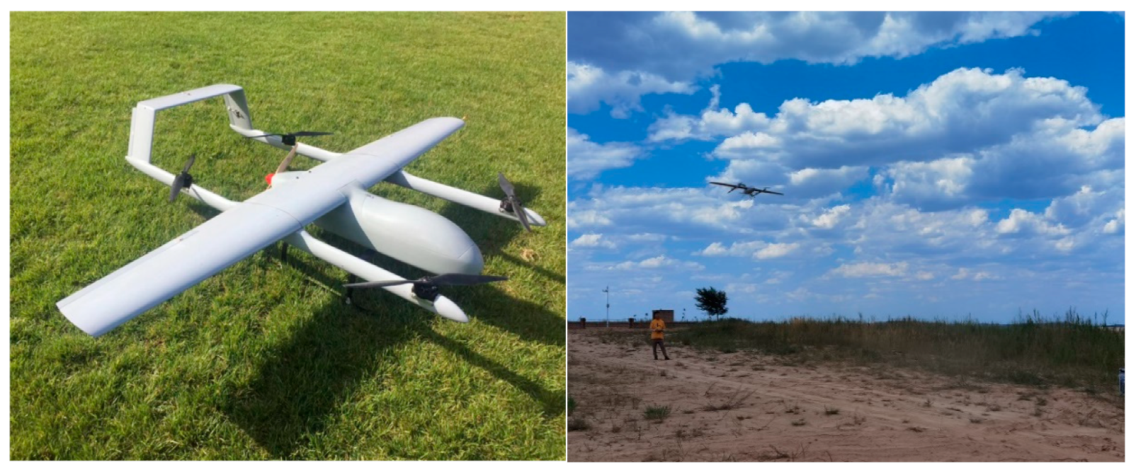
In area coverage path planning, for given dynamics constraints of the UAV, fewer turns generally mean a shorter path. In this paper, a fixed-wing UAV with vertical take-off and landing (VTOL) is used as the carrier to study the problem of regional coverage path planning. Considering the influence of terrain change, in order to simplify the problem, the following reasonable assumptions are made.
(1) The area coverage is set to meet the zoom range requirements of the aerial photography equipment for all encountered to terrain fluctuations, to ensure that the UAV can perform tasks at the same altitude.
(2) The UAV is within the error range during turning and straight-line following, and situations such as gust and sideslip are not considered.
(3) Each area covering the path planning task is a convex polygon (When the shape of the region is a concave polygon, the concave parts are connected to form a convex polygon for processing).
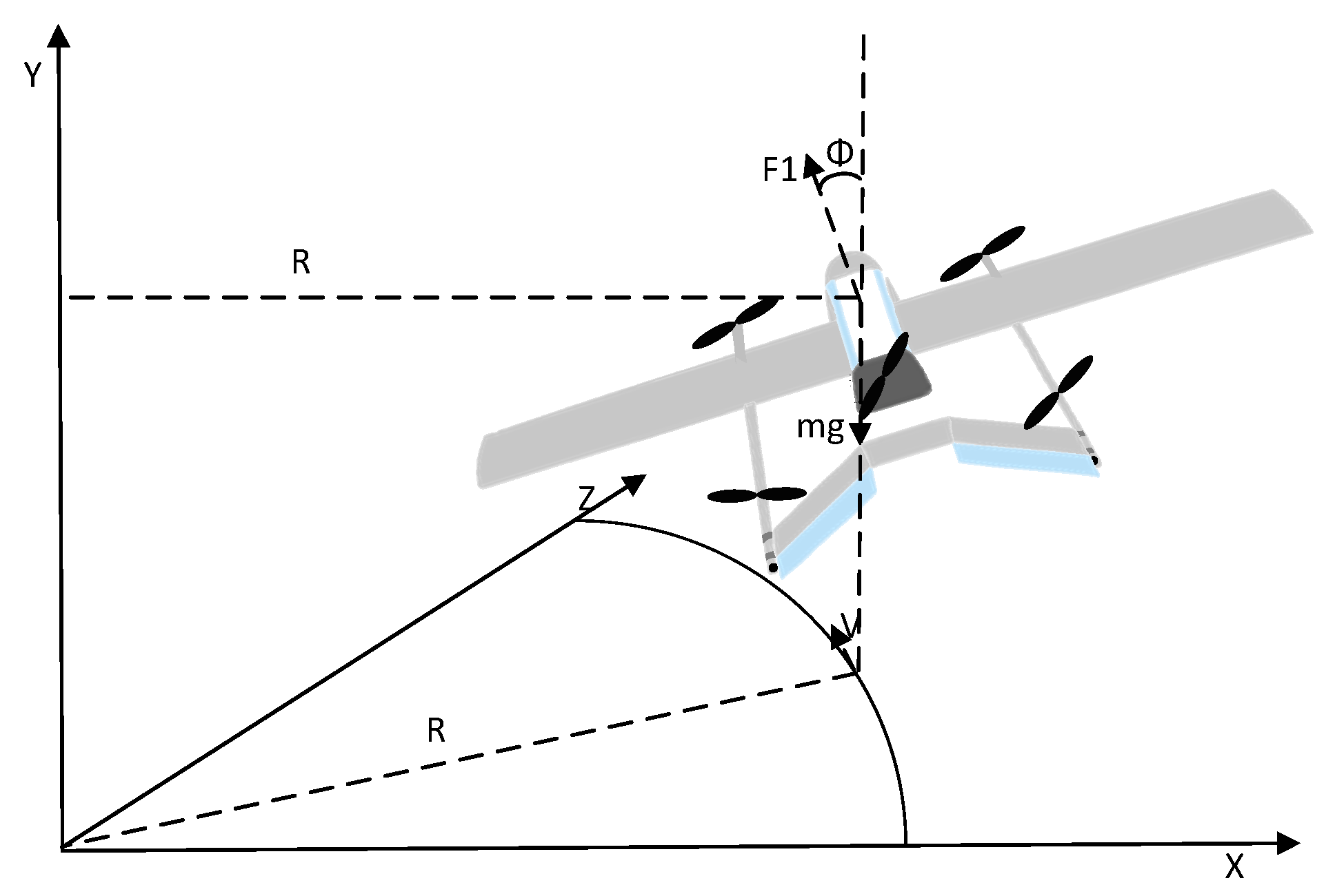
The VTOL UAV is constrained by battery power and cannot switch endlessly between rotor and fixed-wing modes. Usually, the rotor mode is used for take-off and landing, whereas the fixed-wing mode is employed in cruise to save energy. Therefore, path planning of a VTOL UAV should meet its kinematic constraints as much as possible. According to the assumptions above, the UAV coverage path planning can be studied on a two-dimensional plane. When flight speed and load of the UAV are known, only the minimum turning radius constraint needs to be considered. The Kinematic parameters and variable description of the UAV are shown in
Figure 1.
According to
Figure 1, the following relationship can be obtained.
where
is the lift of UAV,
is the mass of the aircraft,
is the gravitational force exerted on the UAV (including airborne equipment),
the rolling angle of UAV,
the minimum turning radius of UAV,
the instantaneous speed of UAV,
, and
the gravitational acceleration. We can also write
To obtain an optimal path, the minimum turning radius should be met during turning.
4. Problem Formulation
A. TSP problem conversion
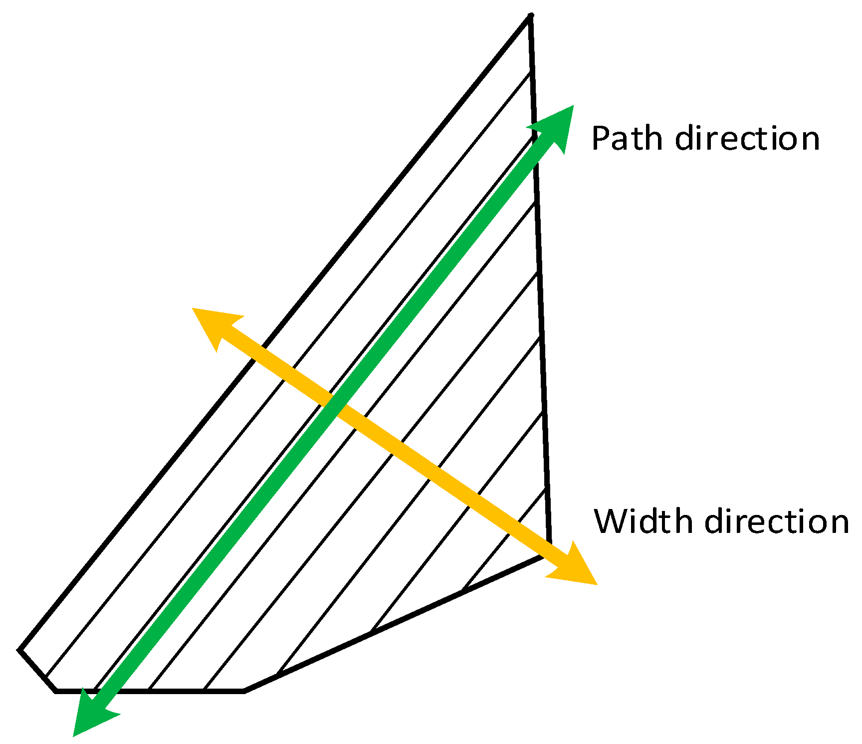
The area that a single fixed-wing UAV can fly under energy constraints is limited. Path planning normal to the width direction of the convex polygon is the optimal strategy [
1], as shown in
Figure 2.
In
Figure 2, the green thick line indicates the direction of the path, and the thick yellow line indicates the width direction. However, if the path is executed in sequence, e.g., one by one from left to right, the UAV needs to fly longer when turning between paths, resulting in excess energy consumption, because the distance between two adjacent paths is less than the minimum turning radius. Therefore, three situations can be considered when turning between adjacent tracks, as shown in
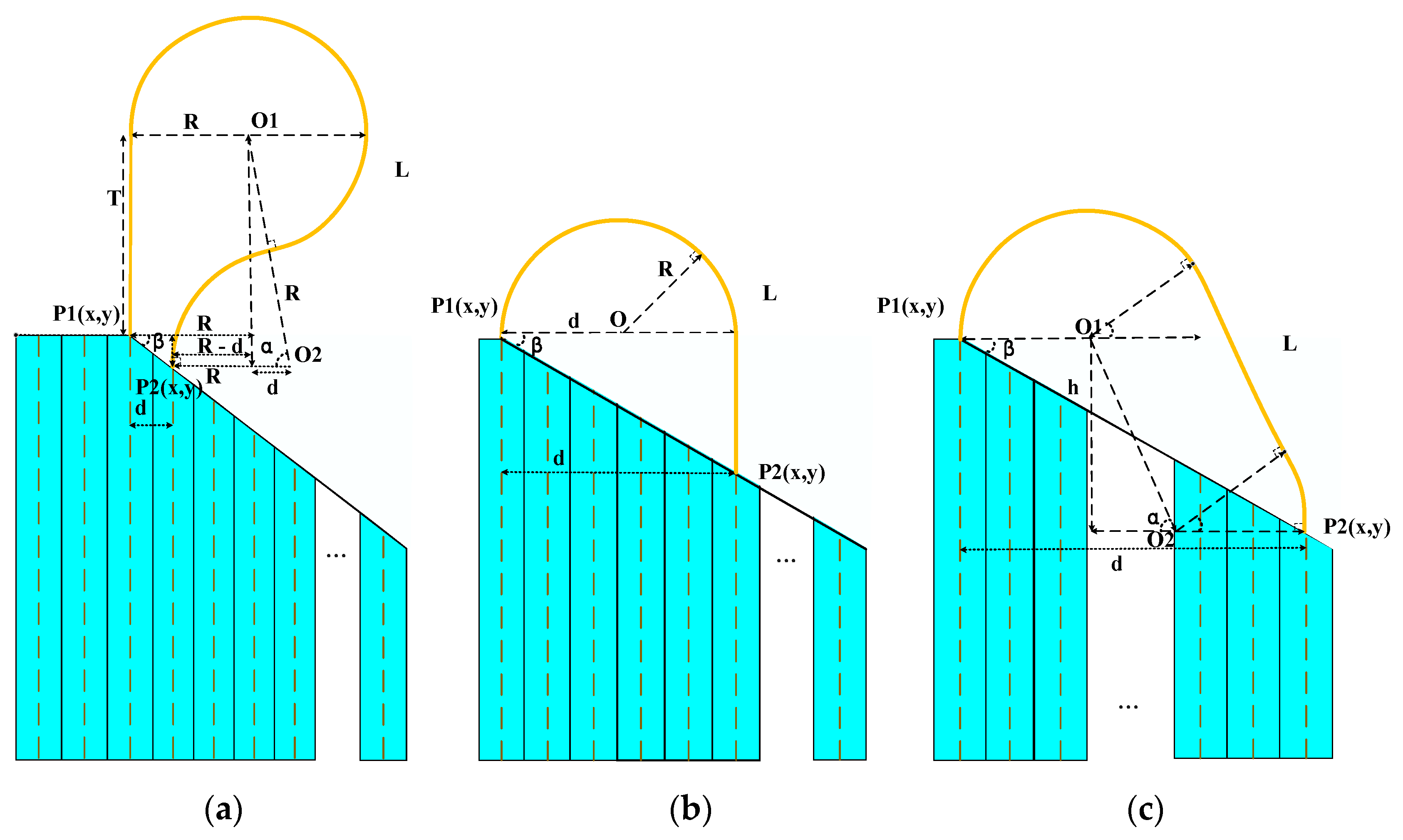
Figure 3.
Three area coverage strategies are shown in
Figure 3, where the dotted line represents the path to be flown by the UAV in the mission area, and the trapezoidal region represents the area covered by each track. The yellow line is the path that the UAV needs to fly outside the mission area. It is obvious that (b) is the best turning strategy. Strategy (c) could be the second best in a certain range. Strategy (a) seems the worst. However, beyond a certain distance range, (a) could be better than (c).
It can be seen from
Figure 1 and
Figure 2 that the regional coverage path planning task can be fulfilled as long as the aircraft can complete these paths, and that different path sequences lead to different path lengths. Another important constraint is that the aircraft would have to take off and land at the same point in practical operation. Therefore, this problem can be transformed into a tsp [
28,
29,
30]. The specific treatment is as follows.
- (1)
number each path in sequence .
- (2)
both ends of each path can be used as either entry point or departure point of that path; whether entry or departure will be determined by the starting point.
- (3)
Calculate the actual distance from one path to another. The distance L is calculated with reference to the annotations in
Figure 2, from the formula below.
where
is the minimum turning radius,
d is the span,
,
,
,
.
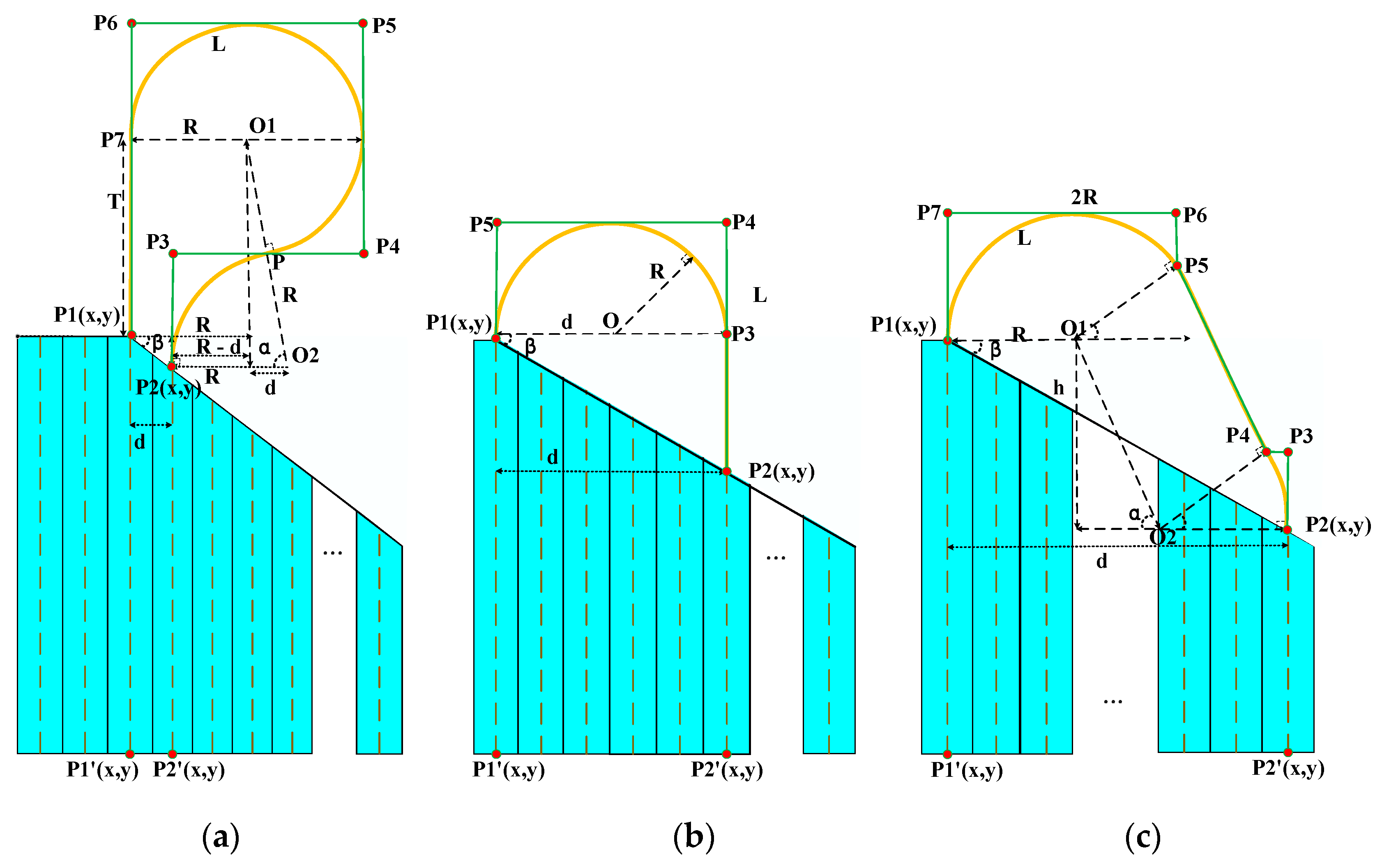
B. Waypoint generation
Since the turning path tracking of the considered VTOL UAV adopts L1 [
31,
32,
33] algorithm we need, therefore, to calculate a reasonable waypoint to ensure that the UAV can fly in the optimal path when turning. Each waypoint reached by the UAV has an acceptance radius; when considering the optimal path, the acceptance radius is equal to the turning radius.
The three cases a, b and c in
Figure 4 correspond to a, b and c in
Figure 3. The pseudo code of waypoint generation is as follows (Algorithms 1 and 2):
| Algorithm 1. . |
| 1:
|
| 2:
|
| 3:
|
| 4:
|
| 5:
|
| 6:
|
| 7:
|
| 8:
|
| 9:
|
| 10:
|
| 11:
|
| 12:
|
| 13:
|
| 13:
|
| 14: |
Ned2Geo converts the Ned (North East Down) coordinate system to the geographic coordinate System, Geo. Geo2Ned does just the opposite.
| Algorithm 2.. |
| 1:
|
| 2:
|
| 3:
|
| 4:
|
| 5:
|
| 6:
|
| 7:
|
| 8: { |
| 9: case 0: |
| 10:
|
| 11:
|
| 12:
|
| 13:
|
| 14:
|
| 15:
|
| 16:
|
| 17:
|
| 18:
|
| 19: break; |
| 20: case 1: |
| 21:
|
| 22:
|
| 23:
|
| 24:
|
| 25:
|
| 26:
|
| 27: break; |
| 28: case 2: |
| 29:
|
| 30:
|
| 31:
|
| 32:
|
| 33:
|
| 34:
|
| 35:
|
| 36:
|
| 37:
|
| 38:
|
| 39: break; |
| 40: default: |
| 41: break; |
| 42: } |
| 43: return
|
5. Improved Genetic Algorithm
Genetic algorithm (GA) belongs to the family of bionic algorithms. It is a random search algorithm based on biological natural selection and genetic mechanisms, with the advantages of parallel search and global optimization [
14].
5.1. Encoding of Individual Genes
After numbering the area coverage paths, it is necessary to access all path numbers without repetition (except for the take-off and landing path numbers). Here, the path numbers are regarded as genes, and the chromosome length of each individual of the population is fixed. Since in an actual operation, the take-off and landing points are always chosen in advance, the starting number of each chromosome is the same.
5.2. Initial Population Generation
Generation of initial population in the conventional genetic algorithm usually adopts the principle of random generation, which is susceptible to falling into local optimization in the iterative process. According to the definition and properties of the good point set [
34,
35,
36], when the integral of the function on the unit cube
in the s-dimensional Euclidean space is approximated by any weighted sum of the function values of any given
points, the resultant error of taking
good points reaches minimum, with a point distribution that is more uniform than those obtained by other means. Similarly, mapping the good points in
space to the solution space results in a solution set that is more evenly distributed and closer to the solution space. In other words, there is a higher chance to obtain the optimal solution. Generally, construction of the good point set is independent of the spatial dimension, overcoming the shortcomings of the orthogonal table design method. It also provides a very good means for high-dimensional approximation. Therefore, in order to improve the solution accuracy, this paper uses the good point set algorithm to construct the initial population, through which a more evenly distributed solution set can be realized in the solution space. In these populations, the evolutionary operation can evolve to the optimal solution with a greater probability than the random population. The steps of constructing the initial population from the good point set are listed below.
- (1)
Let be the unit cube of an -dimensional Euclidean space. Let , ,;
- (2)
Let , where denotes the size of the point set;
- (3)
Let , shaped as , with its deviation satisfying , where is a constant only related to . Then, is considered as a good set of points and is called a good point;
- (4)
Taking , , where is the smallest prime number satisfying , is a good point. If , then is also a good point.
A group of initial populations with uniform distribution can be constructed using the algorithm above. In the solving process, depending on the different population sizes, the calculation results are all floating-point values. In the gene coding, the numbering of paths requires integers. Therefore, the good point set should be rounded, after which duplicate numbered paths will be generated within each individual in the population. Then these duplicates need to be replaced with paths whose sequence numbers are close to those integers that are not in the current numbering list.
5.3. Fitness Function
Genetic algorithm uses the fitness value of individuals in the population to search. Selection of the fitness function directly affects convergence speed of the algorithm and whether the optimal solution can be found. The focus of this study is essentially a distance minimization problem, with a fitness function of
where
denotes each individual, and
denotes the number of genes in individual chromosomes,
denotes the ith gene. The fitness function can be used to measure the advantages and disadvantages of individuals, so that the algorithm can carry out subsequent genetic operation. The distance between different individuals is calculated from Equation (3).
5.4. Genetic Operation
Genetic operation includes three parts: selection, crossover, and mutation. After the initial population is generated, the optimal solution can be sought through iterative genetic operation. In genetic algorithm, the crossover operator is the main operator because of its global search ability, whereas the mutation operator is regarded as the auxiliary operator due to its local search ability. Thus, genetic algorithm has fairly balanced capabilities of both global and local search, as a result of cooperation and competition between crossover and mutation. The so-called cooperation means that when the population is trapped in a hyperplane in the search space and fails to escape by only the crossover operation, the mutation operation can help it jump out of the current limit and make the iteration converge to a better solution. Competition means that when the desired chromosomes have been obtained through cross operation, the mutation operation may damage these chromosomes and degrade individual fitness. The settings of genetic operation in this study are as follows.
5.4.1. Heuristic Crossover Operator
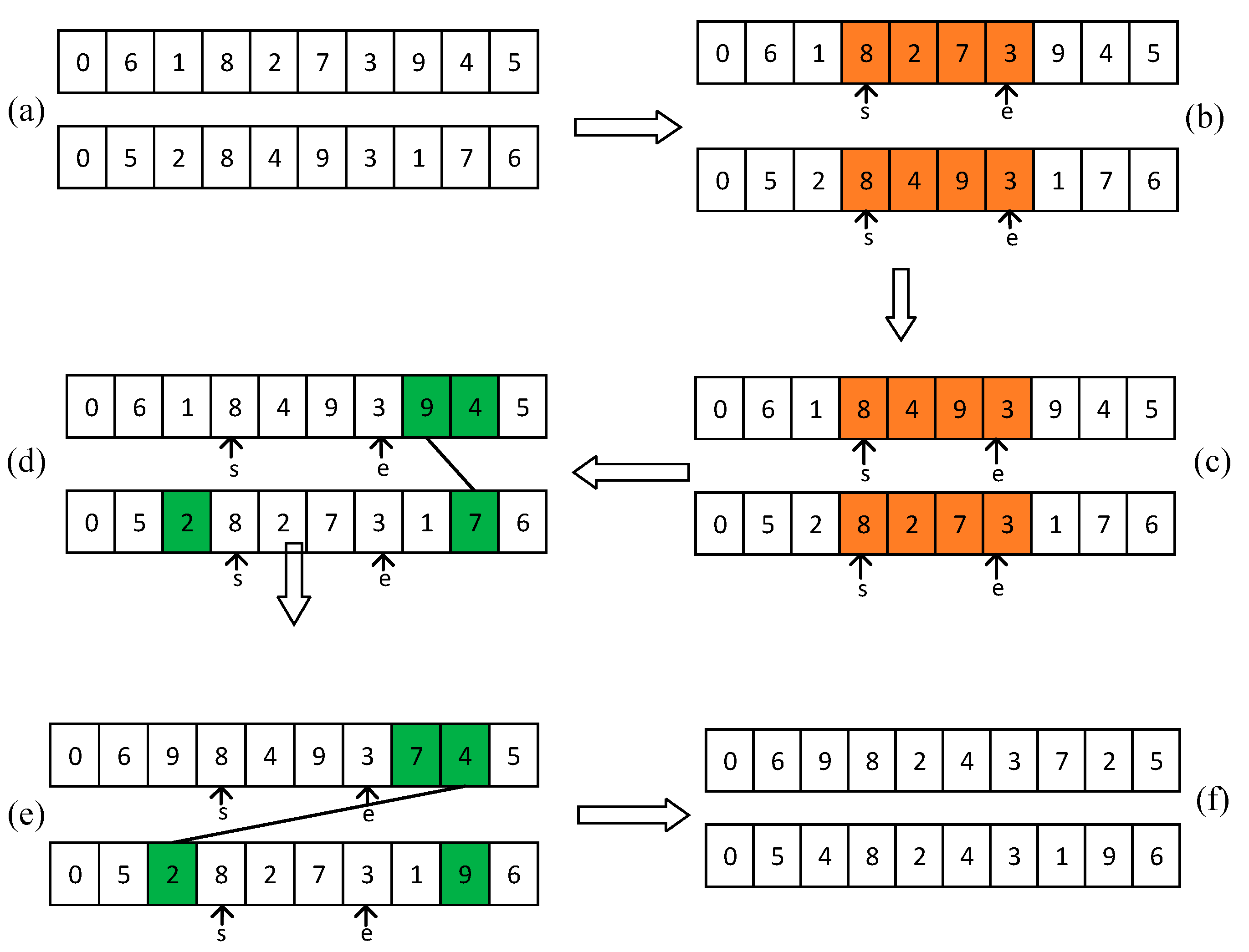
Treat the two gene positions with the largest distance in the chromosome with a large fitness as the initial crossover position, and execute cross operation on them, with the goal of obtaining individuals with better fitness than their parents. As shown in
Figure 5, the specific steps are listed below.
- (1)
Disrupt the existing population order and select two adjacent individuals with the set crossover probability, as shown in
Figure 5a;
- (2)
Select the individual with large fitness value from step (1), and calculate the distance between its two adjacent genes. Select the latter of the two genes with the largest distance as the intersection starting point. As shown in
Figure 5b,
is the intersection starting position, and the corresponding intersection starting position of another chromosome is also
. The intersection ending point can be randomly obtained on the other side of the starting point. As shown in
Figure 5b,
is the intersection end position;
- (3)
Exchange the genes from
to
between the two chromosomes, as shown in
Figure 5c;
- (4)
The duplicate genes in each chromosome are collected from both sides of
and
. Calculate chromosome fitness values. Individuals with a large fitness value are preferentially replaced with duplicate genes, as shown in
Figure 5d;
- (5)
Repeat step (4) until the repeated gene replacement is completed. Now, one of the two genes has a larger fitness value whereas the other has a smaller one. Diversity of the population can be maintained, as shown in
Figure 5f.
5.4.2. Random Interval Reverse Mutation
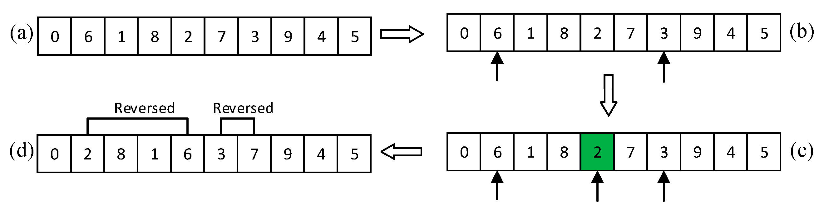
The purpose of introducing mutation in genetic algorithm is twofold. First, to endow the genetic algorithm with the ability of local random search. When the algorithm has approached the neighborhood of the optimal solution through the crossover operator, local random search performed by the mutation operator can accelerate convergence to the optimal solution. Of course, the mutation probability in this case should be set to a small value, otherwise the trend of approaching the optimal solution could be hindered by mutation. Another important function of mutation is to help genetic algorithm maintain population diversity, thereby preventing premature convergence. As shown in
Figure 6, the mutation operation follows the steps described below.
- (1)
Randomly extract an individual from the population with a preset mutation probability, as shown in
Figure 6a;
- (2)
Randomly obtain the start and end position indices for the mutation operation, as illustrated by genes 6 and gene 3 in
Figure 6b;
- (3)
Calculate the middle position index between the start and end position indices (green square in
Figure 6c;
- (4)
Reverse the order of the numbers in two intervals: (a) from the start position index to the middle position index, and (b) from middle to end, in order to obtain the variant individuals, as shown in
Figure 6d.
5.4.3. Tournament Selection
Subsequent to crossover and mutation operations, the current population is a new population, in which the individuals possess a richer diversity than that before the genetic operation. However, since only those population individuals with a large fitness will be selected, the differences between chromosomes tend to be gradually homogenized after several generations. Therefore, the tournament method is adopted here. That is, several individuals are sampled with replacement from the population with a set probability; repeating this operation for many times will result in the scale of the initial population. The specific steps are as follows.
- (1)
Determine the number of individuals for each selection and the number of selections ;
- (2)
Randomly select individuals with replacement from the population, within which individuals with the highest fitness are further selected to enter the offspring population;
- (3)
Repeat step (2) multiple times until the is reached. In other words, the population size should reach the size of the primary population to form a new generation of population.
5.5. Algorithm Description
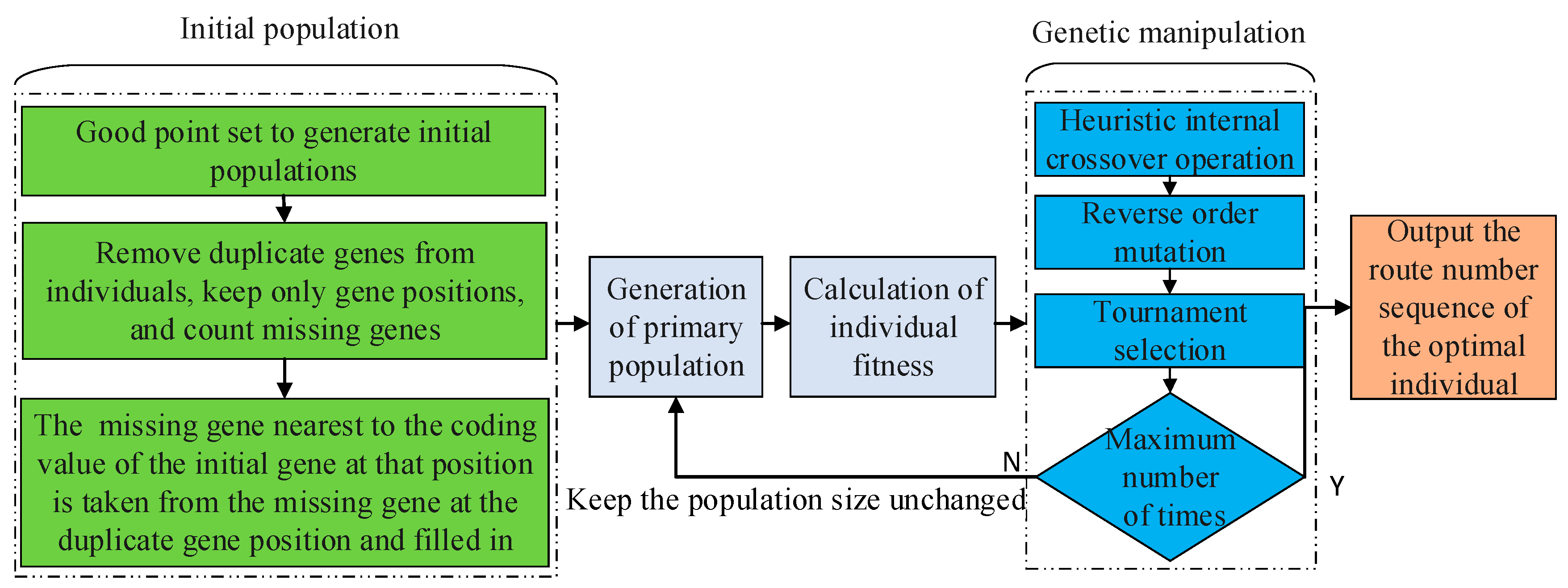
The overall flow of the algorithm proposed in this study is shown in
Figure 7.
Firstly, a uniformly distributed population with
individuals is obtained by the good point set algorithm. Then, a new population is created through crossover, mutation, and selection from the genetic algorithm. After
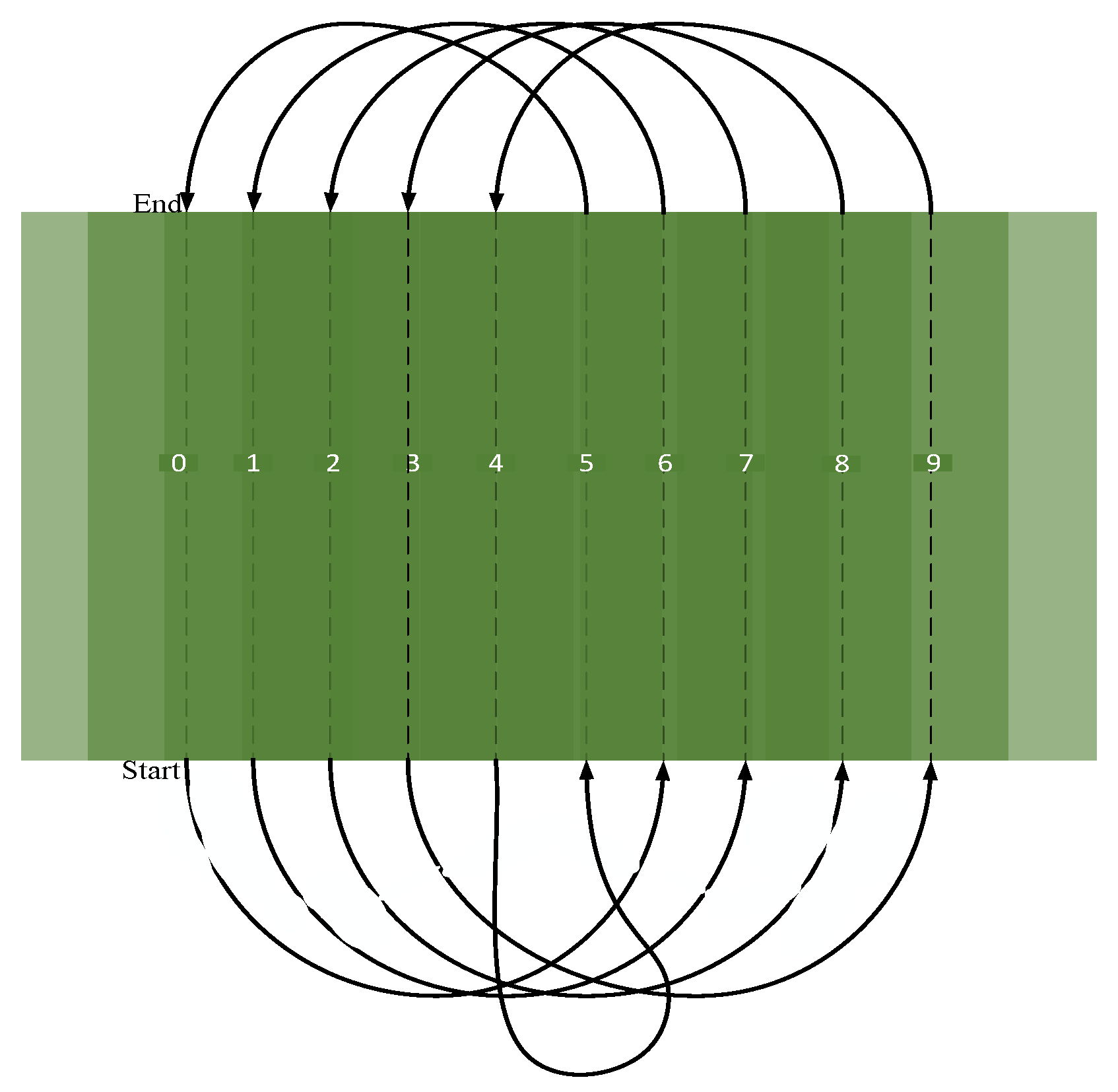
iterations, a population with a high average fitness value can be reached. Individuals with the highest fitness are subsequently selected, which, in other words, give the optimal track sequence number. Finally, by selecting an endpoint from the starting number as the take-off point, the complete track planning can be carried out based the sequence of track numbers. As shown in
Figure 8, the optimal track numbering sequence is 0, 6, 1, 7, 2, 8, 3, 9, 4, 5, 0. Taking path 0 as the starting point, complete planning can be performed accordingly. It is noted that paths 4 and 5 are adjacent paths, and their separation is shorter than the minimum turning radius of the UAV. Therefore, when the UAV enters 5 from 4, planning is conducted according to
Figure 3a; the other two scenarios should follow
Figure 3b,c.
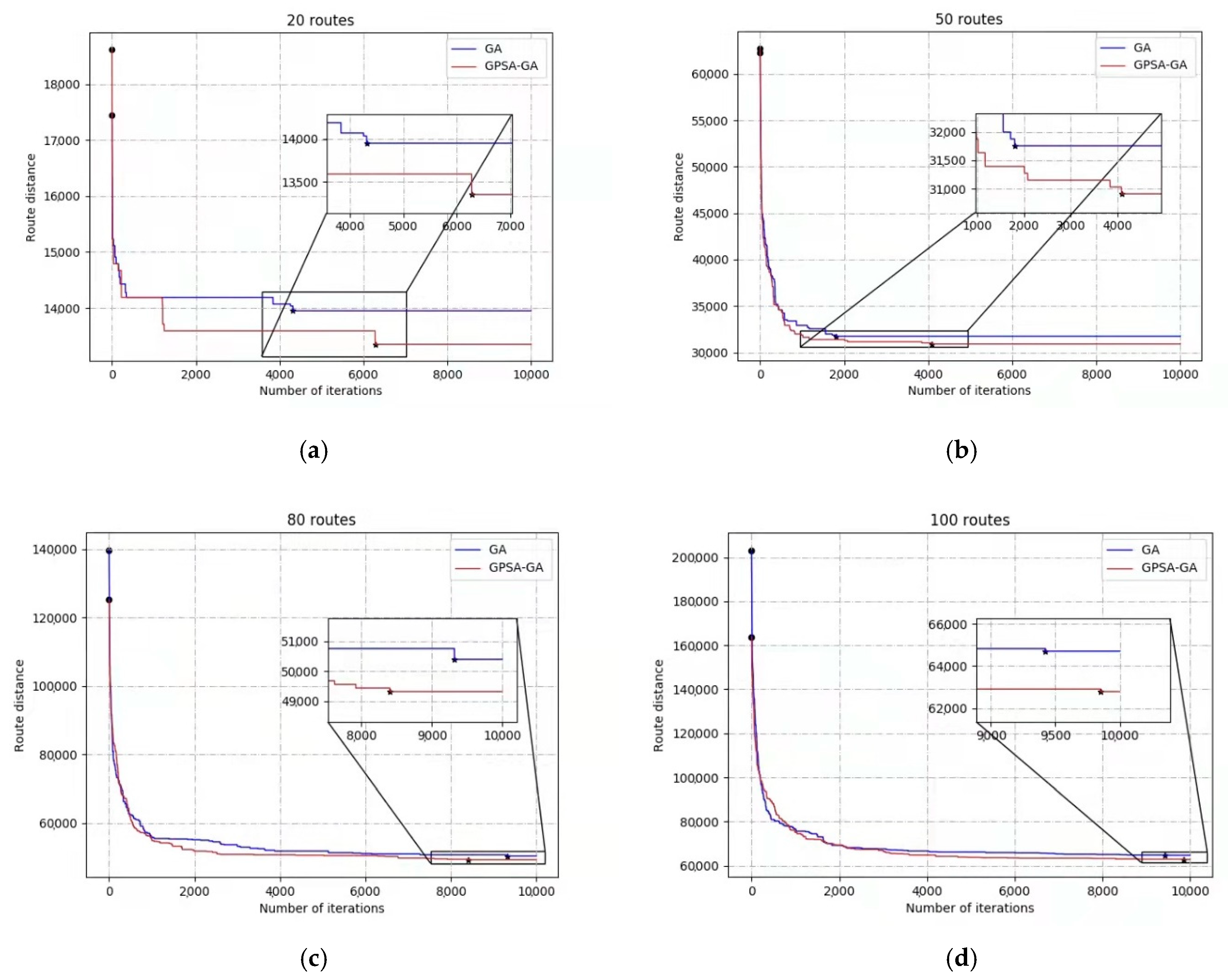
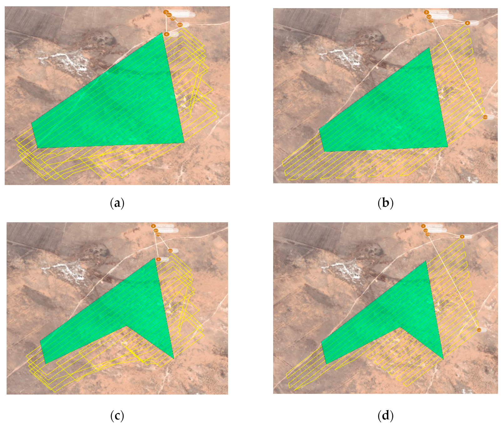
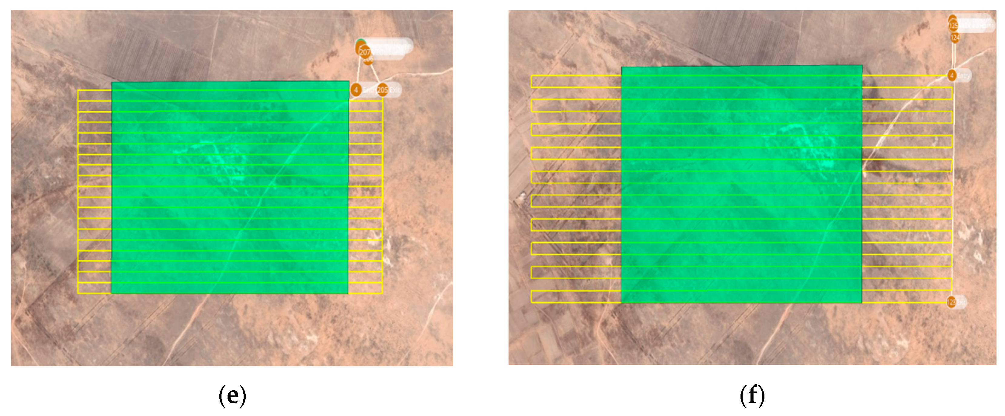
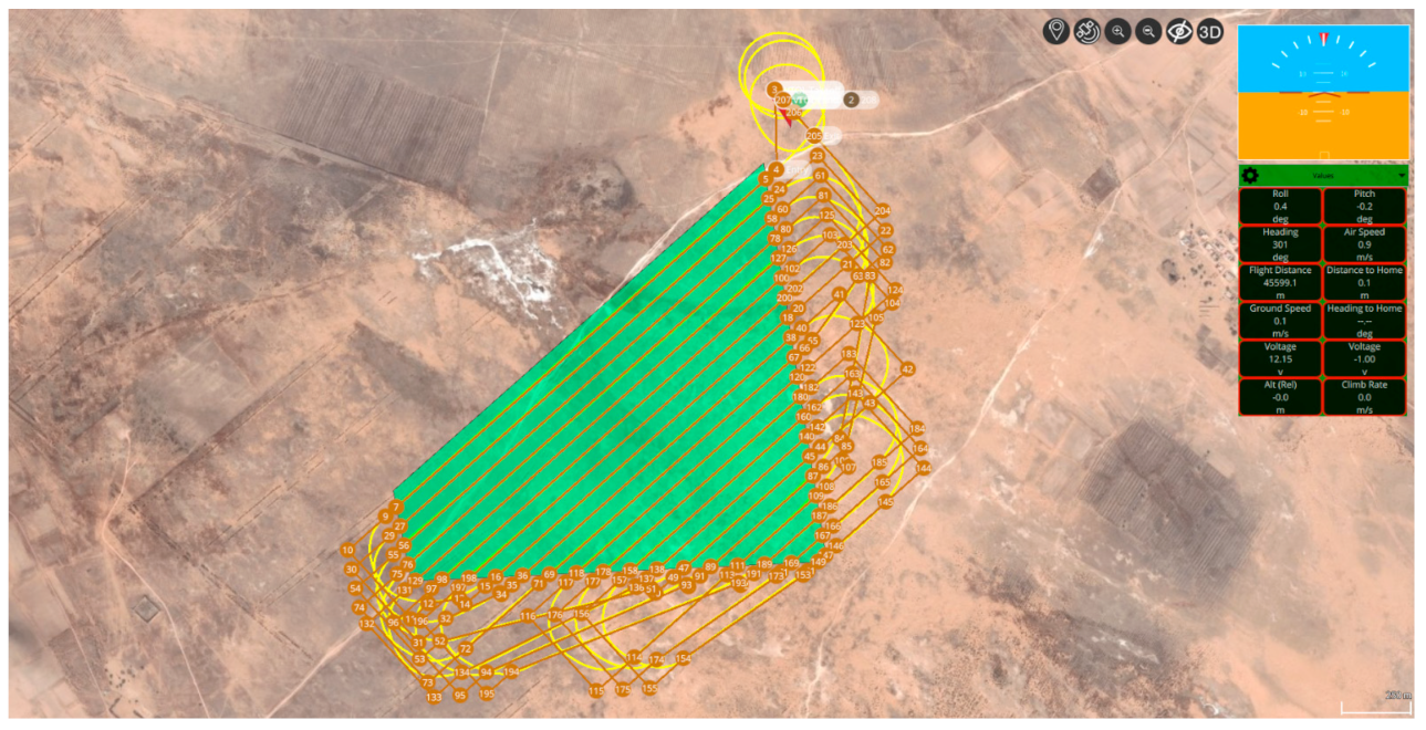
7. Conclusions
Coverage path planning is studied in this work. The regional CPP problem is first transformed into a TSP problem. The combination of good point set and genetic algorithm framework is employed to solve the problem. Simulations are carried out in scenarios of 20, 50, 80, and 100 covered paths. Compared to conventional GA, the proposed algorithm achieves better solutions and, at the same time, the improvement is more remarkable with the increase of the number of paths. This is also verified by the actual flight of 20 and 50 paths. However, increase in the number of paths also leads to the problem that the data size will be squared if the CPP problem is converted to a TSP problem, greatly reducing the convergence speed and increasing the corresponding planning time. In the future, region segmentation algorithms can be used to segment a large area, and algorithms with shorter planning time can be further studied.
In addition, this paper is only based on the coverage path planning of two-dimensional plane, which can be studied in three-dimensional space in the future to achieve better flight effect.


 ,
, 


