1. Introduction
Scientific exploration of small-bodies has attracted much attention and interest during recent decades and plays an important role in the exploration of the Solar System. The successful exploration mission of asteroids 433 Eros and 25143 Itokawa, especially the operation of the Hayabusa 2 spacecraft at asteroid 162173 Ryugu, showed the strong feasibility of operating a spacecraft in close proximity to small-bodies. The causes of these explorations are based on several reasons, such as the exploration of early formation stages of the solar system and planetary defense.
The gravity of an asteroid is very weak, and the irregular gravitational field around an asteroid also perturbs the state of a spacecraft [
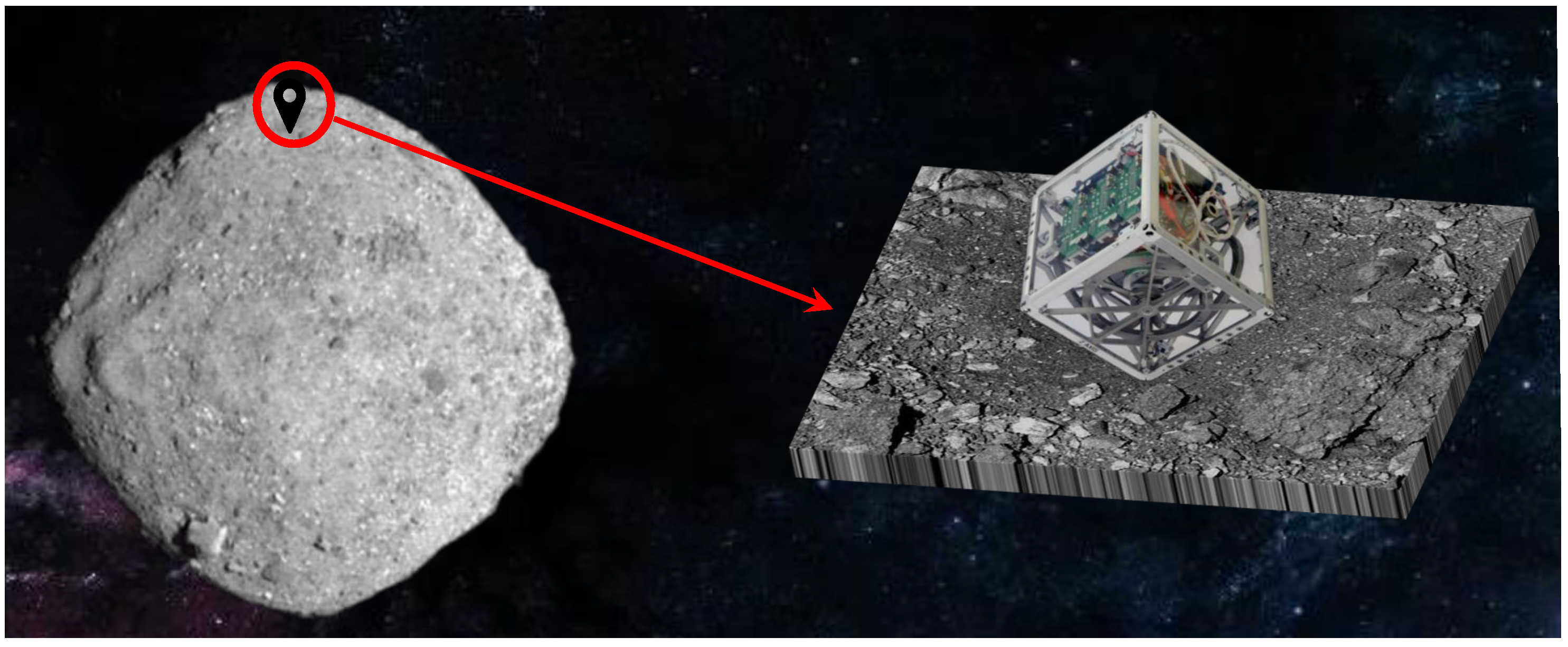
1]. Thus, the traditional roller rover cannot move on the surface of small objects for inspection and detection. Reaction wheel-based pendulum-type Cubli Rovers are suitable as asteroid surface rovers, which can generate jumping behavior by their flywheels or perform a tumbling motion. The use of ballistic jump landing and the tumbling of the detector attitude to achieve the movement of the surface of the asteroid has gathered increased interest. The main advantage lies in the long-range and large-area detection on the surface of small-bodies can be achieved by jumping. Meanwhile, the attitude and position of the rover can be moved by internal angular momentum exchange, which is mechanically simple and easy to implement without chemical propulsion and is not affected by a dusty environment. There are two kinds of ideas for the tumbling and jumping patrol in literature. One is to drive an external mechanical structure to contact the surface of the star to generate a rebound force [
2]. On the other hand, the collision between the spacecraft and the surface of the small celestial body produces a rebound force [
3]. In [
4,
5,
6], the satellite on-orbit attitude control process around small celestial bodies and the gravity field of small celestial bodies are investigated. The Philae lander of the ESA Rosetta mission and the MINERVA-II and MASCOT small ballistic jump landers of the Japanese Hayabusa 2 mission have successfully conducted small-body jump landing tests [
7,
8]. However, the Cubli Rovers are suitable as jump probes on the surface of asteroids and no relevant studies have been found in the open literature.
In the current literature, there have been investigations on Cubli [
9]. The Cubli is similar to the 3-D inverted pendulum system, and a 3-D inverted pendulum system [
10] was gradually evolved. Different from the linear trolley control in the traditional inverted pendulum, the 3-D inverted pendulum often used a three-axis flywheel and housing to form a momentum exchange system. It was originally developed by ETH Zurich as a 15 cm × 15 cm × 15 cm robot that can stably stand upside down with one vertex of a cube and can jump and roll. In terms of control, in [
9], the vertical position control of the Cubli one-dimensional prototype was first performed using the LQR method. In [
11], the dynamics of 3-D systems were modeled based on Kane’s equations, and a system identification method was provided, using LQR for stable control of the linearized model. Ref. [
12] proposed an optimal-size cube robot based on parameter optimization, and through feedforward control, it achieved self-balancing stability. A feedback controller was proposed based on the backstepping method for balance control [
13], and the feedback linearization was used to design the controller to track the take-off trajectory segment. Ref. [
14] used the Lagrangian method and Kane method to establish an attitude control model and verified the validity of the model through simulation. To maintain the balance on the Cubli frame, an LQR controller based on a Lagrangian derivation of the dynamics was designed, which utilized the state variables of the frame angle and its angular acceleration, as well as the wheel angle and its angular acceleration [
15]. A method for feedback control using quaternions to describe attitude is proposed in the literature [
16]. An adaptive robust control is presented to balance the uncertain Cubli system on its corner in the literature [
17]. However, in the existing kinds of literature, the special environment of the asteroid surface and the angular velocity limitation have not been considered, and the dynamic performance requirement has been not considered yet.
A so-called prescribed performance control (PPC) method to ensure the prescribed performance output has been proposed in [
18]. Two robust adaptive control schemes for single-input single-output (SISO) strict feedback nonlinear systems possessing unknown nonlinearities, capable of guaranteeing prescribed performance bounds are presented in this paper [
19]. In [
20], a universal, approximation-free state feedback control scheme is designed for unknown pure feedback systems, capable of guaranteeing, for any initial system condition, output tracking with prescribed performance and bounded closed-loop signals. This paper [
21] investigates the issue of control design for a class of nonlinear systems with guaranteed prescribed performance. In [
22], the authors present a performance-guaranteed adaptive asymptotic tracking control scheme for a class of nonlinear systems with an unknown sign-switching control direction. The study [
23] develops a novel robust distributed estimation algorithm, capable of achieving practically zero average tracking error even for fast time-varying reference signals. The PPC method is beginning to attract the attention of researchers in various fields and it is also widely used especially in the aerospace field. The PPC has been applied in satellite attitude control [
24] and flight vehicles [
25]. In [
26], based on the novel performance function and error transformation constraints, the attitude tracking error is converted into a new error system that guarantees the desired transient and steady-state responses for the tracking error. In this paper [
27], a nonlinear disturbance-observer-based fault-tolerant attitude control scheme is developed for the combined spacecraft with prescribed performance. Performance in the light of convergence time, stability and accuracy with inertia uncertainty, actuator saturation and external disturbance can be prescribed.
The PPC approach, as a control methodology to conduct the dynamic or transient performance of the system, provides a new idea for the control system design of Cubli Rovers. Thus, inspired by the PPC method, the paper presents an adaptive PPC for reaction wheel-based Cubli Rovers to ensure the success of the balance control, and meanwhile, the avoiding jumping condition is also considered. The main features of this paper are twofold:
(1) An adaptive prescribed performance control scheme is proposed for the attitude system of reaction wheel-based inverted pendulum-type Cubli Rovers in the environment of the asteroid to achieve fine transient performance in the balancing motion. Asymptotic stability of the tracking errors is guaranteed even under uncertainties.
(2) Based on the knowledge of attitude dynamics, the avoiding jumping condition in the specific gravitational field in the asteroid is analyzed and the proposed control is guaranteed not to leave the ground via the small angular velocity.
The rest of this paper is organized as follows.
Section 2 formulates the attitude model for the balancing control for Cubli Rovers and the gravitational field and avoiding jumping condition are analyzed in detail in
Section 3. The main theoretical results about the adaptive prescribed performance control are given in
Section 4.
Section 5 provides simulation results and
Section 6 concludes the paper.
2. Problem Formulation
2.1. Attitude Model of Reaction Wheel-Based Inverted Pendulum-Type Cubli Rovers
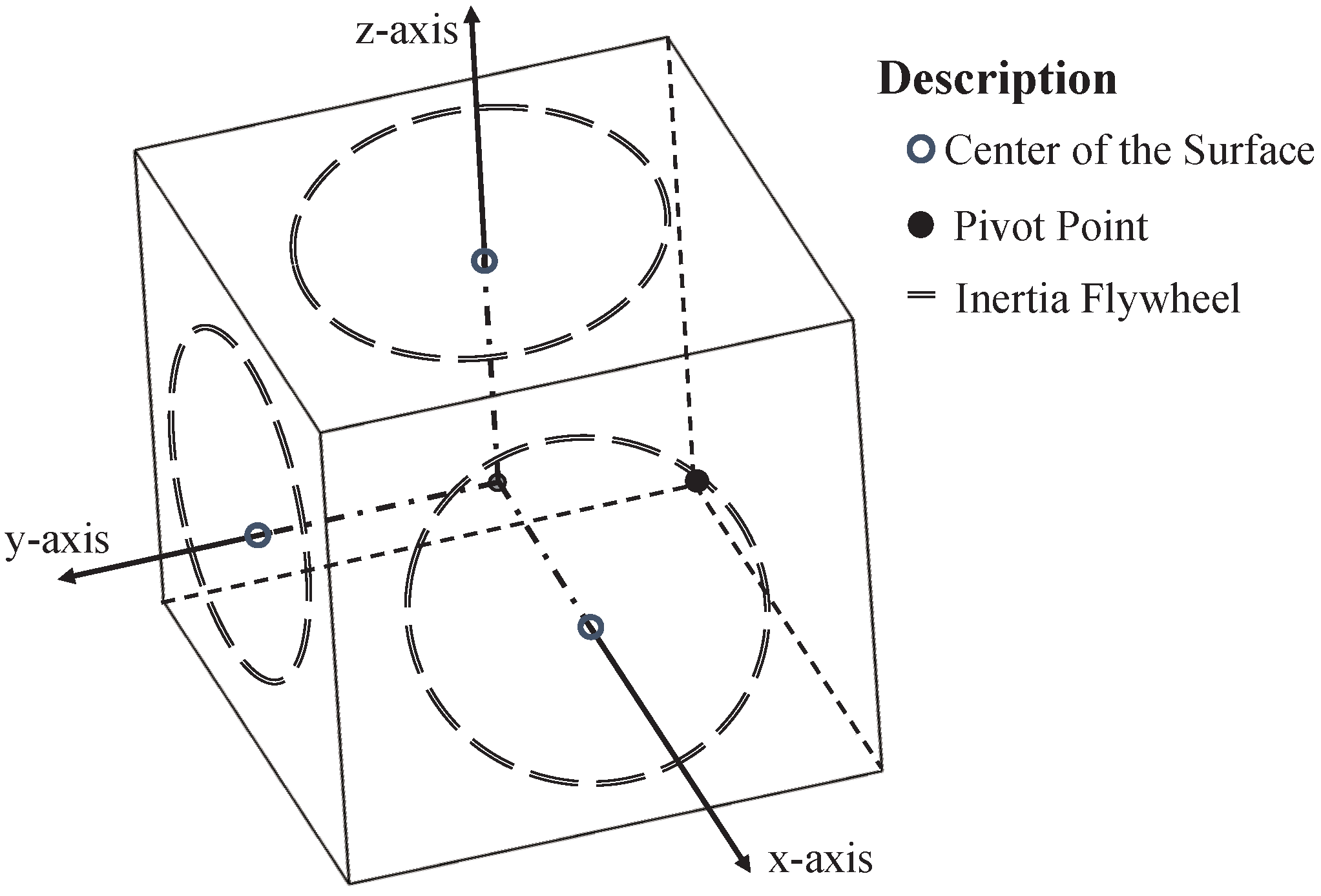
The stable stationing of Cubli Rovers on the surface of an asteroid can be formulated as a single-point self-balancing problem. In this part, the attitude model of reaction wheel-based pendulum-type Cubli Rovers is presented for the balancing control. The three momentum wheels of Cubli Rovers are equipped orthogonally on adjacent edges, and the center of mass of the momentum wheels is located at the geometric center of the cube face, as shown in
Figure 1.
Without loss of generality, the model can be appropriately simplified, and it is considered to increase the load on the surface without the momentum wheel to ensure that the cube center of mass coincides with the geometric center, and it can be considered as a symmetrical geometry. Considering the three-degree-of-freedom problem of fixed-point rotation of a rigid body, it is possible to establish the body fixed frame o-xyz with the origin located at the center of mass and the three coordinate axes passing through the center of the geometric surface, respectively.
The coordinate system is established as shown in
Figure 2 and the body-fixed frame is used as the inertial frame O-XYZ by selecting the equilibrium position. The Cardan transformation sequence 1-2-3 is used for the transformation between the body-fixed frame to the inertial frame, and the pitch, yaw and roll angles
are obtained as the attitude angles to describe the attitude of Cubli Rovers. The transformation matrix from the inertial frame to the fixed body frame can be expressed as follows
Furthermore, the dynamics of the attitude angles can be represented by the angular velocity which is shown as follows
According to the Lagrangian mechanics method [
13] and the moment of momentum theorem, one has that
where
is the total momentum of the system without the flywheel momentum,
represents the moment generated by gravity on the rotation point of the system, and
represents the moment generated by the flywheel. The term
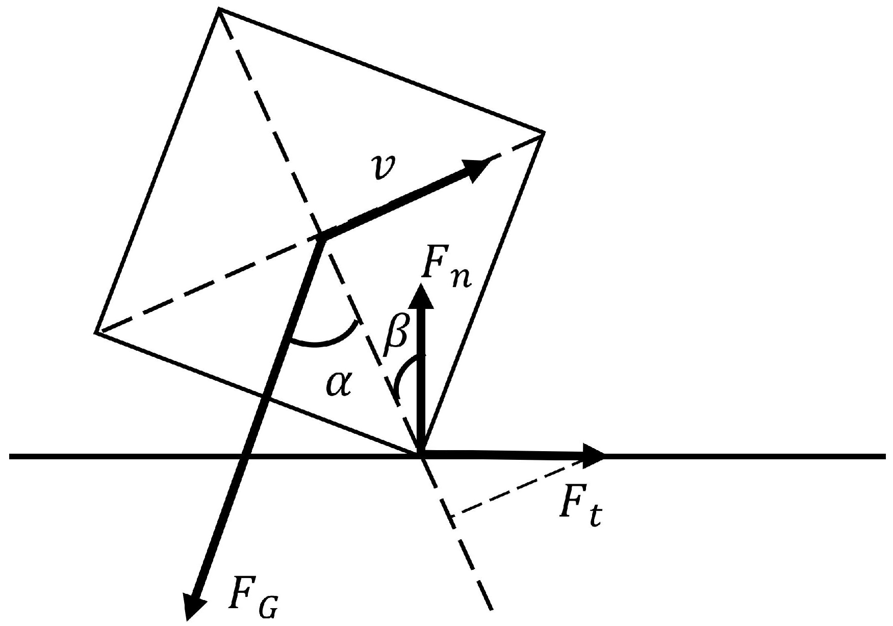
represents the resultant torque generated by external disturbances. Note that the possible relative sliding of the ground pivot point is ignored in this paper. According to the moment of momentum theorem, the rate of change of the momentum of the system is equal to the torque produced by the external force acting on the system
where
r represents the vector radius from the position of the center of mass to the pivot point,
m represents the total mass of the Cubli Rovers,
l represents the side length, and
represents the gravity vector at the current position.
Define
as the rate of change of the triaxial angular velocity of the shell, and then one has that
, where
denotes the moment of inertia of the shell. Since the axial direction is defined as the geometric center passing through the side, the inertia products of the inertia tensor matrix
,
,
are ideally set as zero. Therefore, the system model of the attitude rate can be expressed as:
where
represents the disturbances. The flywheel torque
is used as the input of the system, which has the dynamic characteristics of the flywheel, that is, the limit and the saturation of the flywheel speed. Finally, the attitude model of reaction wheel-based inverted pendulum-type Cubli Rovers is obtained by (
2) and (
5).
2.2. Balance Control Issue in Asteroid
Based on the above modeling procedure, the model of traction wheel-based inverted pendulum-type Cubli Rovers is expressed as a multi-variable nonlinear second-order system with disturbances. The task of the balance control is to ensure the stability of the Cubli Rovers when they are set up. It is important for the mission of the rover on the asteroid. However, the balancing control investigated in this paper is different from that on Earth due to the following reasons:
(1) For the Cubli Rovers, the main concern is whether the attitude angle and angular velocity achieve satisfactory dynamic performance. The introduction of a flywheel as the actuator will cause some problems with speed saturation and instantaneous impulse limitation. In addition, due to the three-axes coupling, it is necessary to ensure that the overshoot of the angular velocity of each axis cannot be large to avoid affecting the effective control of other axes, which puts forward performance requirements for the control method.
(2) Due to the existence of a special gravitational field on asteroids, the effect of gravity plays an important role in the balancing control for Cubli Rovers. Unlike the common gravitational field on Earth, the non-uniform gravitational field affects the system balance if the attitude inclination cannot meet the small steady-state error, so the performance requirement of steady-state error is proposed. On the other hand, in the asteroid environment, the centripetal force provided by gravity is limited, so the angular velocity magnitude should be limited at all times during the rotation to avoid the Cubli Rovers from leaving the ground.
Consequently, the dynamic or transient performance of the balancing control for Cubli Rovers, including the overshoot, steady-state error and setting time, is the main focus that determines the mission on the asteroid. Dynamic performance requirements depend on a pre-designed time-varying function with the ability to assign performance limits throughout the procedure. Therefore, time-varying constrained performance functions are applicable for the control design and thus can ensure that multiple performance requirements are met. To sum up, the control goal of the paper is to steer the attitude angles tracking the desired references with the tracking errors always into the preassigned performance functions.
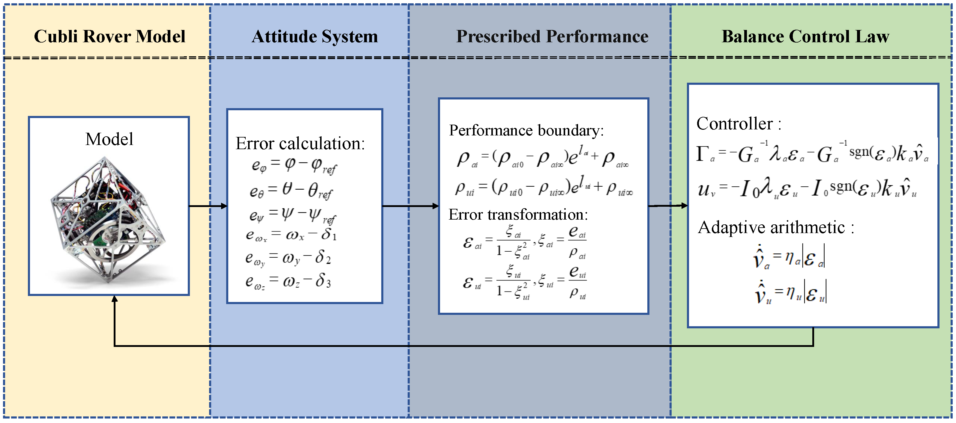
4. Balance Control Based on Adaptive Prescribed Performance Control
4.1. APPC Design
At the expected target position, the inertial frame and the body fixed frame should coincide, that is, the attitude angles
,
,
are zero. Then, the values of tracking target signals are set as
,
,
. Then, the tracking errors of the attitude angles are represented as
For the attitude angle system, the angular velocity can be viewed as the input and a virtual input
for the attitude angle is obtained by
Define the angular rate tracking virtual input state errors as follows
Taking the derivatives of the tracking errors yields that
Design the following virtual control law for the subsystems (
13)
where
,
,
,
,
,
,
,
,
,
, where
.
represents the ratio of the state error to the performance function. When
, we can deduce that
. They need to be converted to unconstrained variables by using non-linear transformation relations
. The performance functions are chosen as
, where the constants
.
For the angular rate subsystem (
14), the actual control law can be designed as
where
,
,
,
,
,
,
,
, where
.
represents the ratio of the state error to the performance function. When
, we can deduce that
. They need to be converted to unconstrained variables by using non-linear transformation relations
. Similarly, the performance boundary functions are set as
where the constants
.
Schematic diagram of the proposed control method is shown in
Figure 4.
Remark 1. The singular point of the matrix is located at . Considering the actual situation of Cubli Rovers, even when the body is stationary on the ground, will not reach the singular point. Therefore, the matrix is always invertible.
4.2. Stability Analysis
This part provides the stability analysis of the proposed APPC law. The necessary theorem is given and explained as follows:
Theorem 1 ([
36]).
Let be an open set with positive constants . Consider the switched system:where is piecewise continuous and uniformly bounded in t and locally Lipschitz on x; q is the switching signal, which takes its values in a finite set and is the number of subsystems. Suppose that the state of the system Equations (13) and (14) does not jump at the switching instants. Then there exists a unique and maximal solution on the time interval where . Theorem 1 shows that the state must remain in a domain if the initial value lies within a finite time interval. the assumption in Lemma 1 about no jumps at the moment of switching is to ensure the continuity of the state, which is necessary and quite important to guarantee that the constrained performance function is not violated. Note that the switching action takes place in the controller, as shown in the formulation of the control law. In other words, the switching occurs on the right-hand side of the dynamic equation, and therefore, does not cause a jumping action of the state. Therefore, the assumption is reasonable in this paper. This theorem is important for performance-guaranteed control design. Of course, we hope that T can be set as , but it may be not satisfied for any case. In this paper, the proposed control law can ensure , which is proven by Theorem 1. Therefore, the basic thought of the proof is described as follows. Firstly the existence and uniqueness of a maximal solution for a time interval is ensured. Then, in the following theorem, we prove that the proposed control scheme guarantees, for : (i) the boundedness of all signals in the closed-loop system; (ii) seek a contradiction to lead to . Finally, we prove that the proposed adaptive control law is analyzed in the following theorem.
Theorem 2. Consider the system model Equations (13) and (14) and the proposed adaptive prescribed performance control Equations (15) and (16). Assuming that Assumptions 1 and 2 hold, the following statements are satisfied: - (1)
All signals of the closed-loop system are globally bounded;
- (2)
The relations are satisfied;
- (3)
The error converges to zero asymptotically, that is as .
Proof of Theorem 2. Invoking the novel adaptive prescribed performance control (
15) and (
16), into the system (
13) and (
14) yields the closed-loop system as follows:
where
and the function
is represented as
Note that the trajectory of the system (
19) is continuous at the switching instants, and thus, the existence and uniqueness of a maximal solution
is guaranteed on the time interval
according to Theorem 1.
Select the Lyapunov function as:
where
,
is an unknown constant. Taking the derivative of
yields that
for the
component in the vector, define an extraction vector:
, used to extract the quantity of
active channels in the system model. According to the expression of (
13) and (
15) one has that
where
, because
and
are bounded variables and the former is always greater than zero and the latter is always less than zero, then it follows that
Therefore, the expression of
is rewritten as
where
. Integrating
over the time range
one has that
that is,
it means:
According to (
25) and (
26), we know that:
and
are established for all
.
Next, for the
component in the vector, the Lyapunov function is selected as
where
,
is an unknown constant, and the derivation process is similar to (
21).
For the
,
component in the vector, define an extraction vector:
,
i means that the element at position
i in the vector b is equal to 1 and the elements at the remaining positions are 0, used to extract the quantity of
,
active channels in the system model. According to (
13) and (
15) we have that
where
. Since
and
are bounded variables and the former is always greater than zero and the latter is always less than zero, which leads to:
Therefore, the expression of
is:
where
, integrating
over the time range
one has:
that is,
it means:
According to Equations (
32) and (
33), we know that:
and
are established for all
.
Finally, let us select the Lyapunov function as
where
,
is an unknown constant, and the derivation process is similar to (
21). Then it follows that:
Define an extraction vector:
,
i means that the element at position
i in the vector b is equal to 1 and the elements at the remaining positions are 0, used to extract the quantity of
active channels in the system model. According to the expression of (
14) and (
16) one has that
where
, because
and
,
,
,
are bounded variables, which leads to:
Therefore, the expression of
is:
where
, Integrating
over the time range
one has:
that is, for
it means:
According to Equations (
40) and (
41), we know that:
and
are established for all
. It is deduced by contradiction that
, that is
for all
. Moreover, it is deduced from (
15) and Equation (
16),
is bounded.
According to (
31), (
34) and (
39) that
is bounded. By applying Barbalat’s lemma, it is deduced that
that is
and
. In summary, the tracking errors converge to zero asymptotically and meets the preset dynamic performance requirements, and the proof is completed. □
4.3. Parameters Tuning
The control law represented by (
15), (
16) consists of the conversion error
,
, the estimate of the adaptive parameter
, and the control parameters
,
,
. In this section, the role and effects of the various parameters involved in the control law are explained. The positive constant
is the gain coefficient of
, which responds to the response of the input signal to the previous state error or the tracking error. If the value of
is increased, the feedback of the control input to the error becomes larger accordingly.
is worth a reasonable increase to accelerate the convergence of the error, but if the value of
is too large, it will lead to an increase in the amount of overshoot and even lead to error overshoot causing system instability. If the
value is too small, it may cause insufficient control input leading to system instability. Then the positive constant
and
are the gain coefficient of the adaptive parameter
and its derivative
. The value of
reflects the effect of the adaptive parameter on the control input, and
determines the rate of change of the adaptive parameter. The main role of the adaptive parameter is to regulate the steady-state error of the system and to make the system asymptotically stable. The values of
and
reflect the effect of the adaptive parameter on the error for compensation. Therefore, improving the steady-state performance of the system, i.e., accelerating the convergence of the steady-state error within a certain time, is the main function of the adaptive parameters.
As mentioned above, the three parameters , , play the role of regulating the speed of error convergence, the steady-state error, and the variation of the adaptive parameters. In the boundary function, the three values , , are the initial value of the boundary function, the convergence rate of the function, and the final convergence boundary that is the final value. The design of the three parameters constrains the trend and the range of the state error, and the existence of the boundary function is the main reason for the selection of APPC in this paper, and the angular velocity constraint in the special environment of the asteroid is achieved by designing the boundary function.
5. Simulation Results
The simulations are divided into four parts. The first subsection shows the simulation results for the Cubli Rovers on Earth and the second part demonstrates the effectiveness of the proposed control method for the environment on the asteroid. The third section shows the effect of changes in each parameter of the APPC controller on the control performance. In the last part, the method in this paper compares the Backstepping method [
37] and the PD control method and provides the comparison results and discussion to show that the APPC method can make the system reach the steady state well, and shows good control performance in the control process, which can be well adapted to the requirements of the asteroid microgravity environment. Thus, it is demonstrated that the proposed method in this paper is superior to the Backstepping method and PD control method.
5.1. Simulation Results and Discussion on Earth
The target attitude angle is all
, The initial angular velocity of Cubli Rovers is
. The initial attitude angle is set to
,
,
. Gravitational acceleration
, total mass is 2 kg, cube side length is
. The values of performance boundary functions and control parameters in the simulation are shown in the following
Table 1.
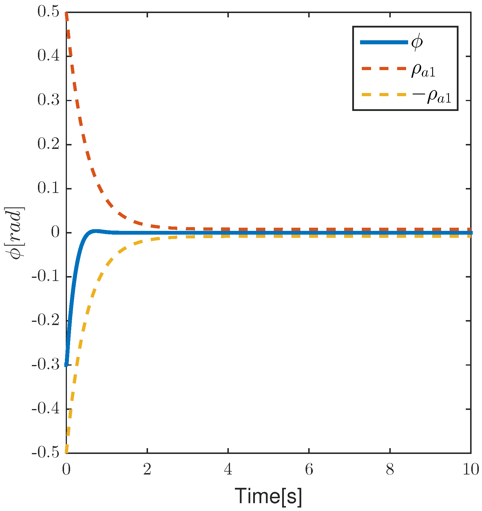
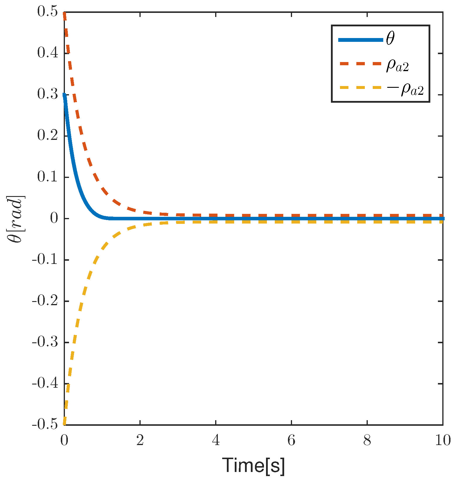
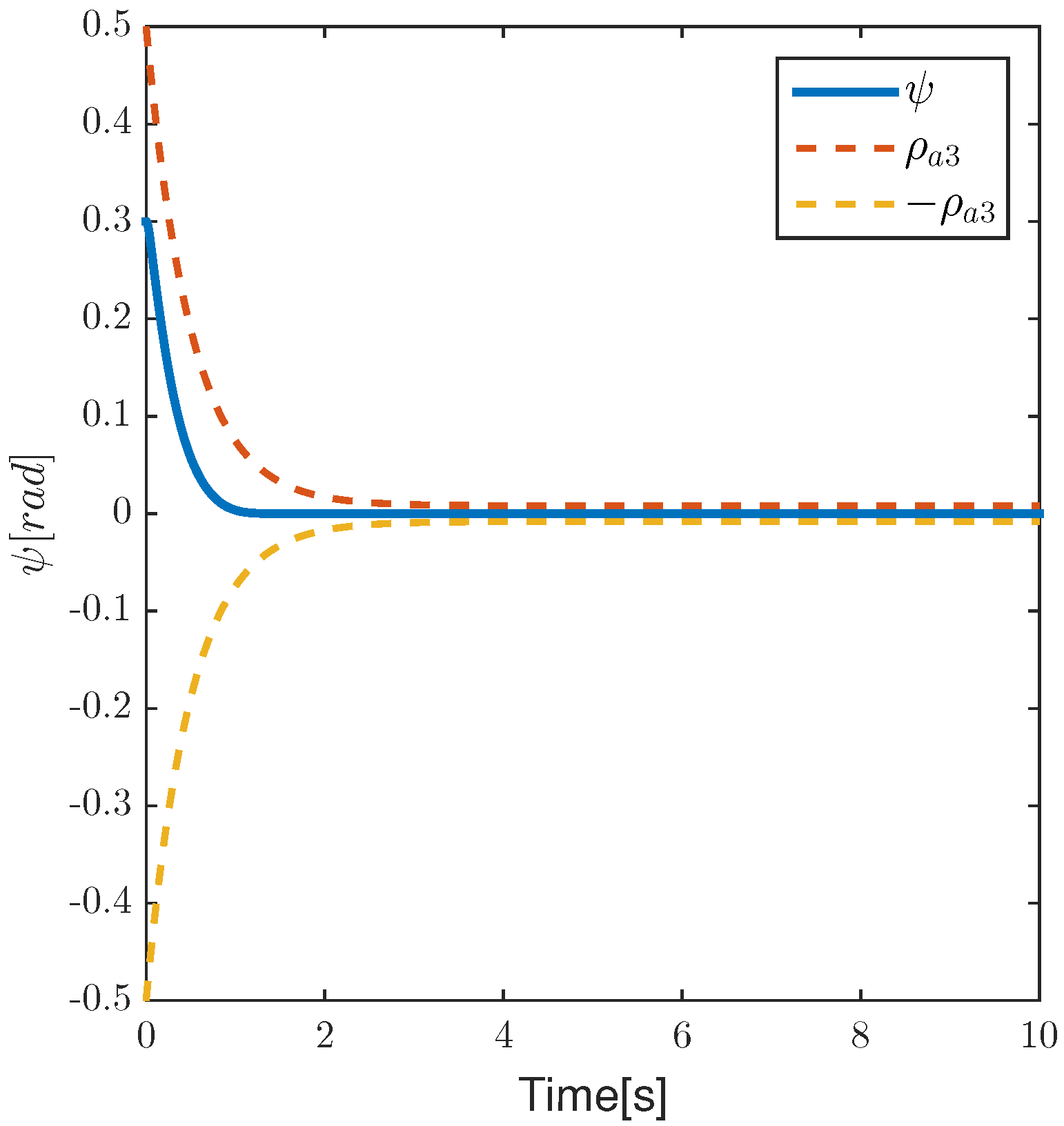
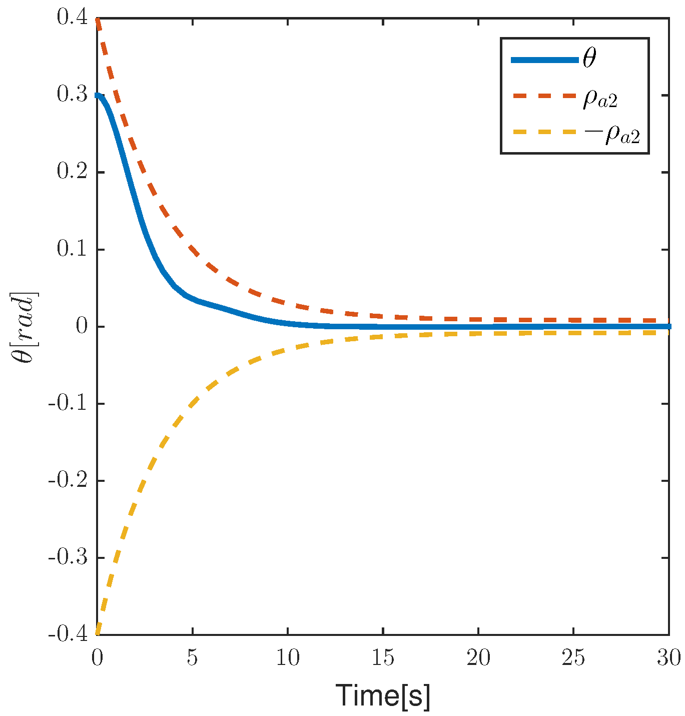
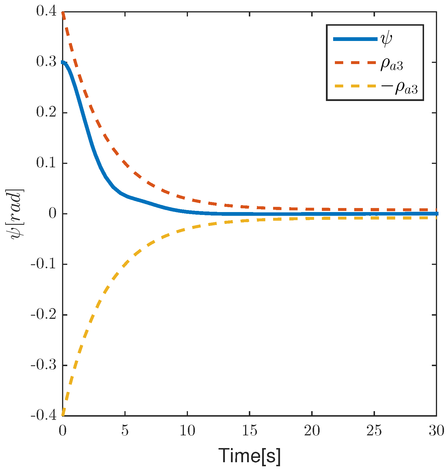
Figure 5,
Figure 6 and
Figure 7 show that the dynamic change curve of the attitude angle in the process, which is also the dynamic performance of the attitude angle error. It can be seen that the attitude angle tracking error has always been within the prescribed performance range of the boundary function. When
,
, successfully converged to zero, ensuring that the key indicators of steady-state error and convergence rate in the prescribed performance function. As seen in
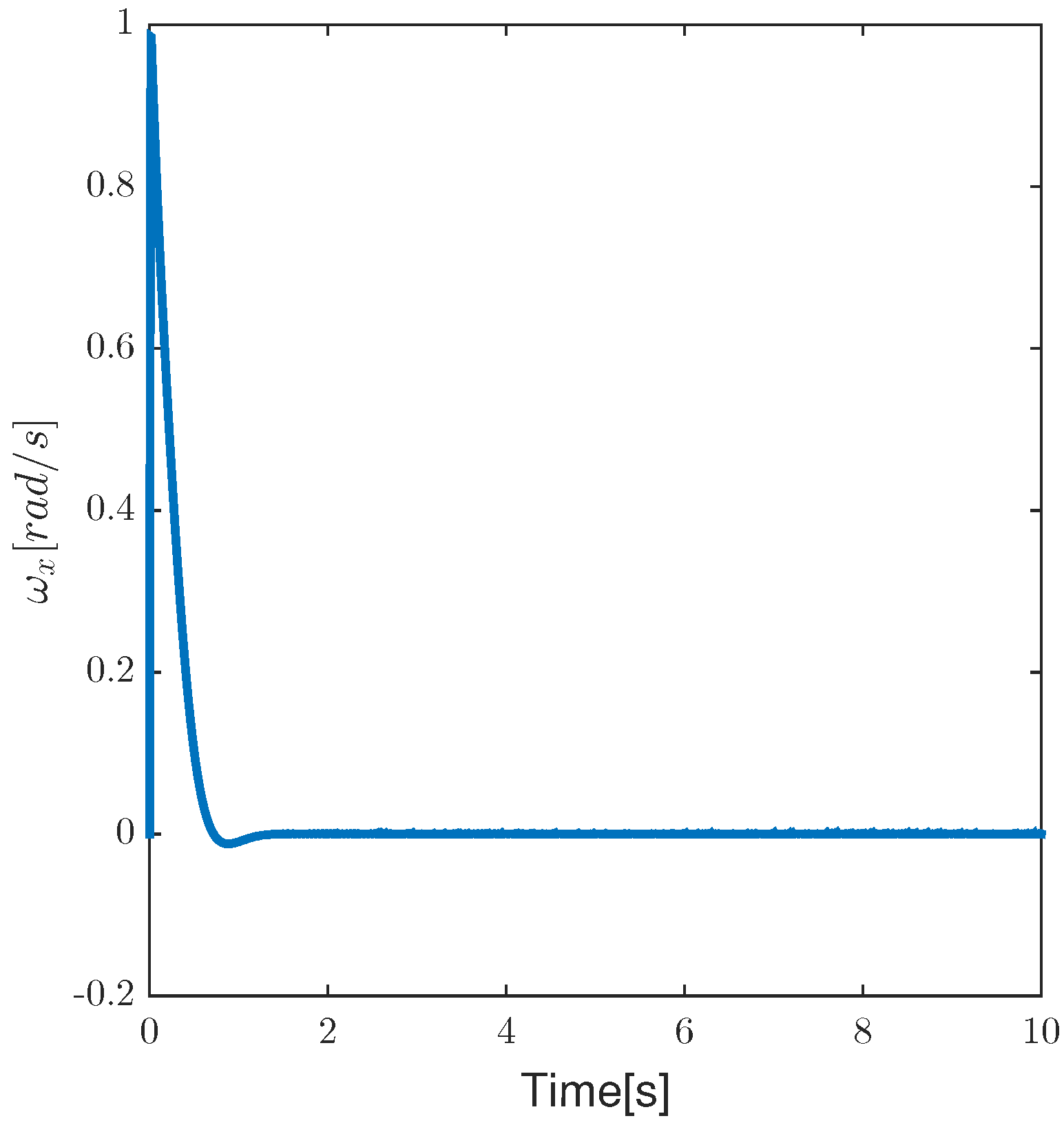
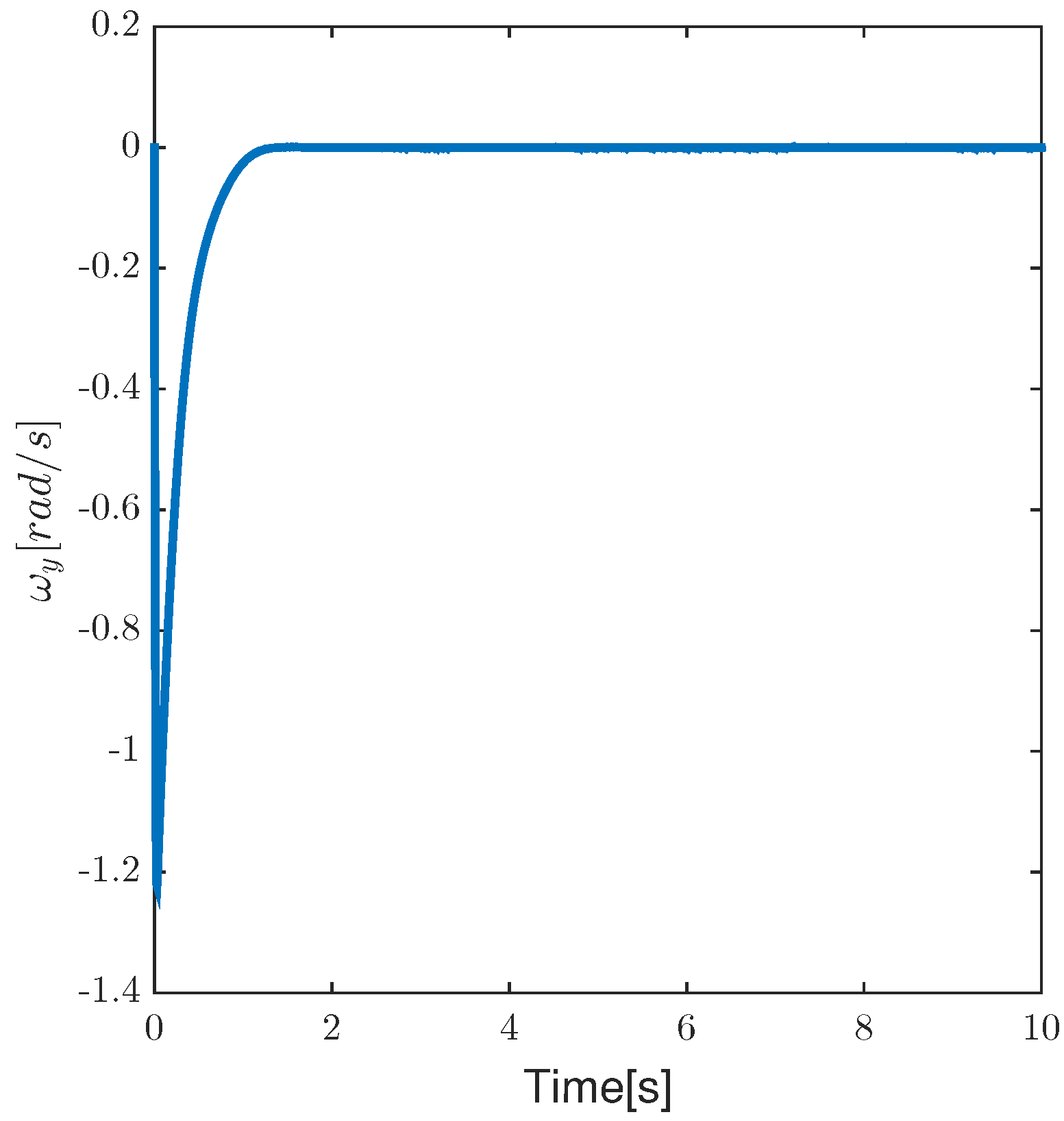
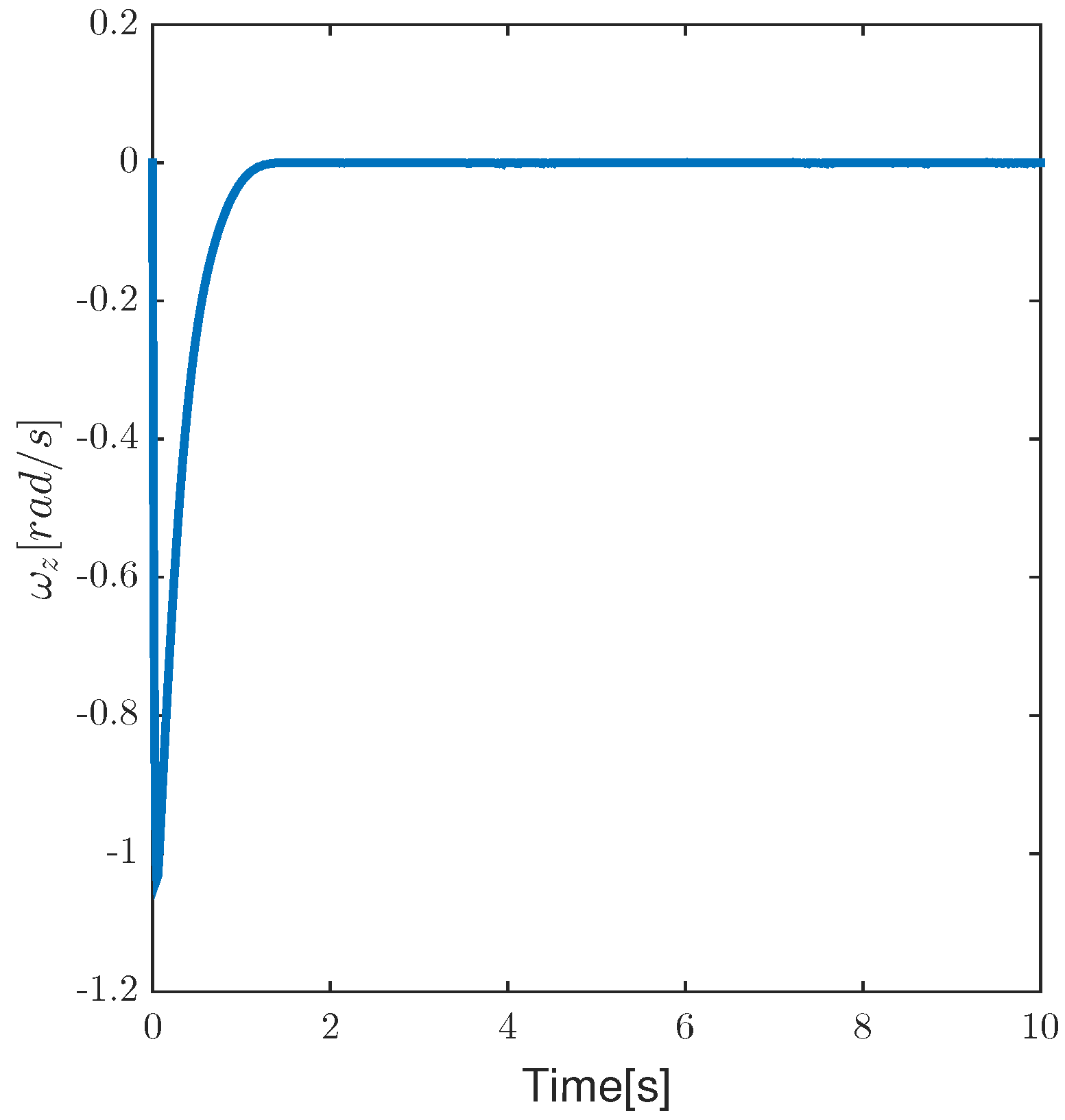
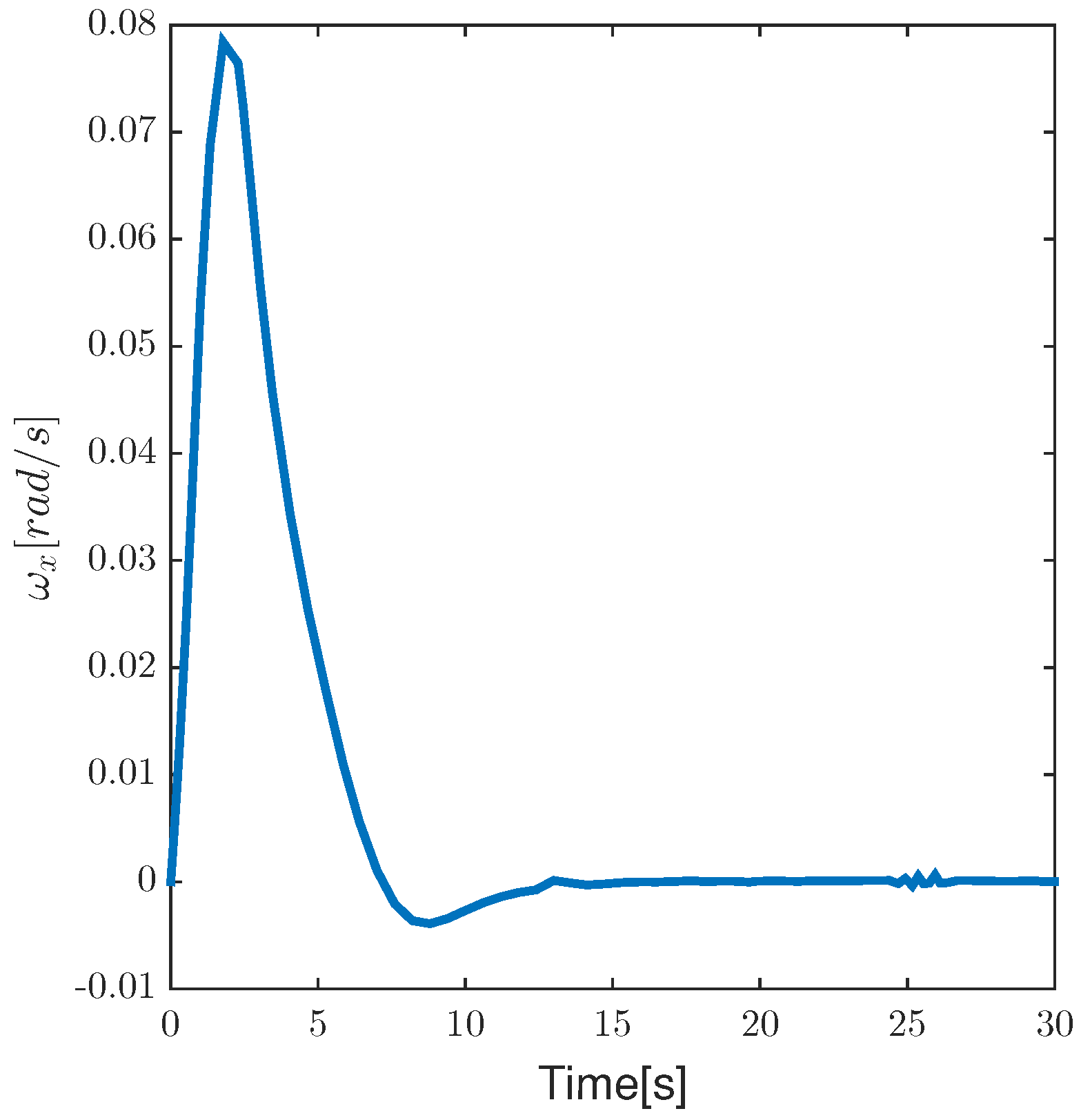
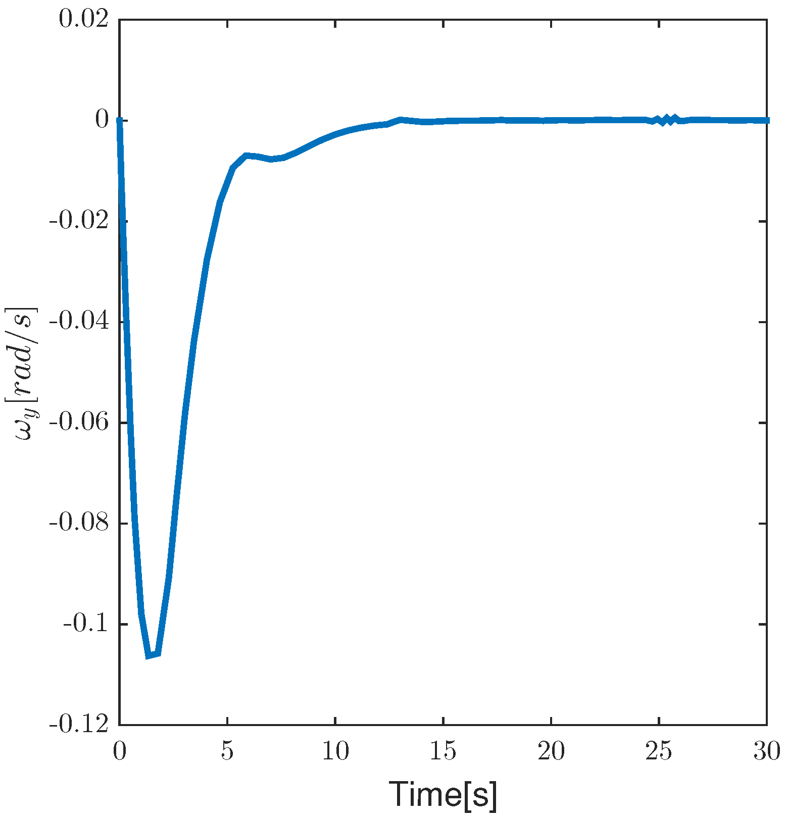
Figure 8,
Figure 9 and
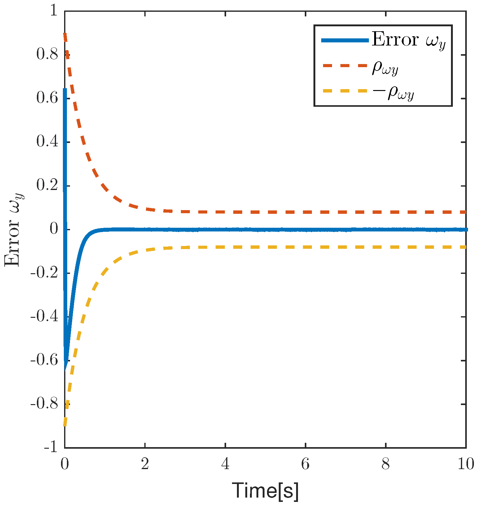
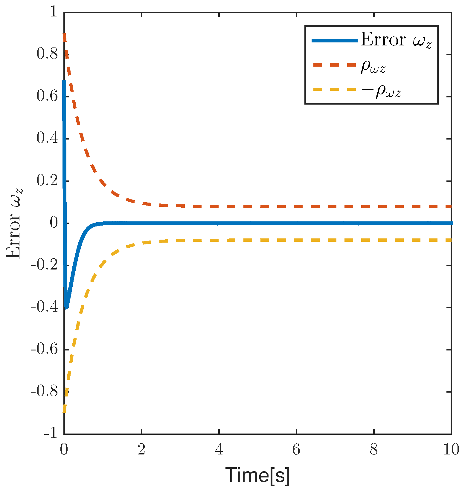
Figure 10, it can also be seen that the three-axis angular velocity variation curves during the control process. As seen in
Figure 11,
Figure 12 and
Figure 13, it can be seen that the tracking error is always within the prescribed performance range of the boundary function, which meets the requirements of the control rate. As seen in
Figure 14,
Figure 15 and
Figure 16, it reflects the input value of the entire system, that is, the input torque generated by the flywheel. It can be seen from its peak value and time that it meets the actual flywheel operating conditions.
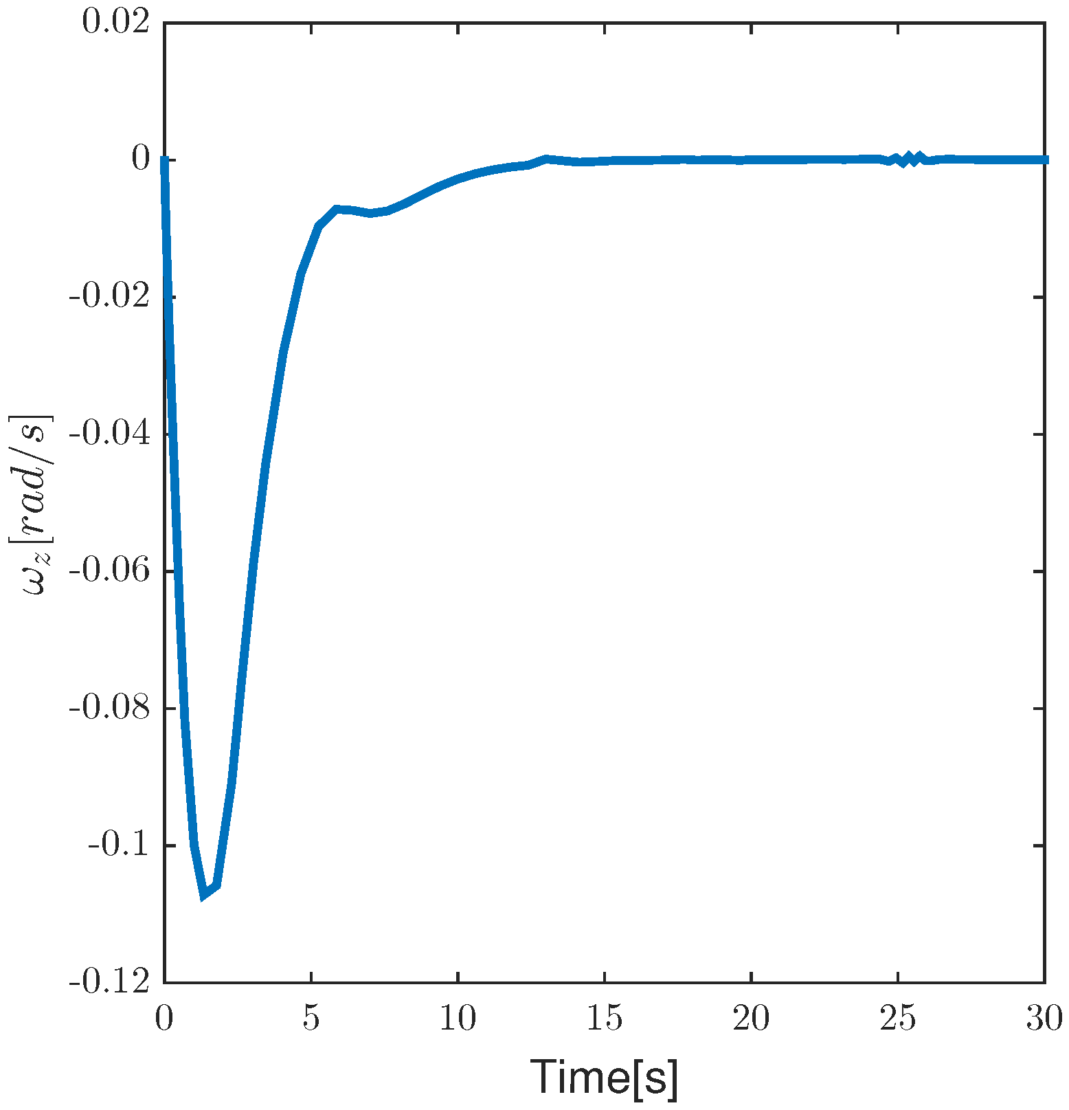
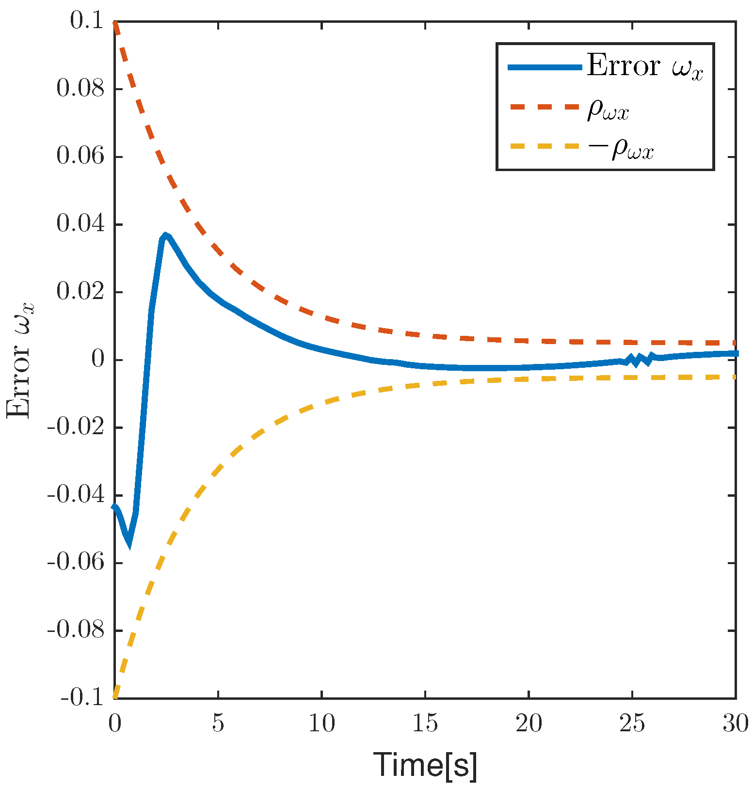
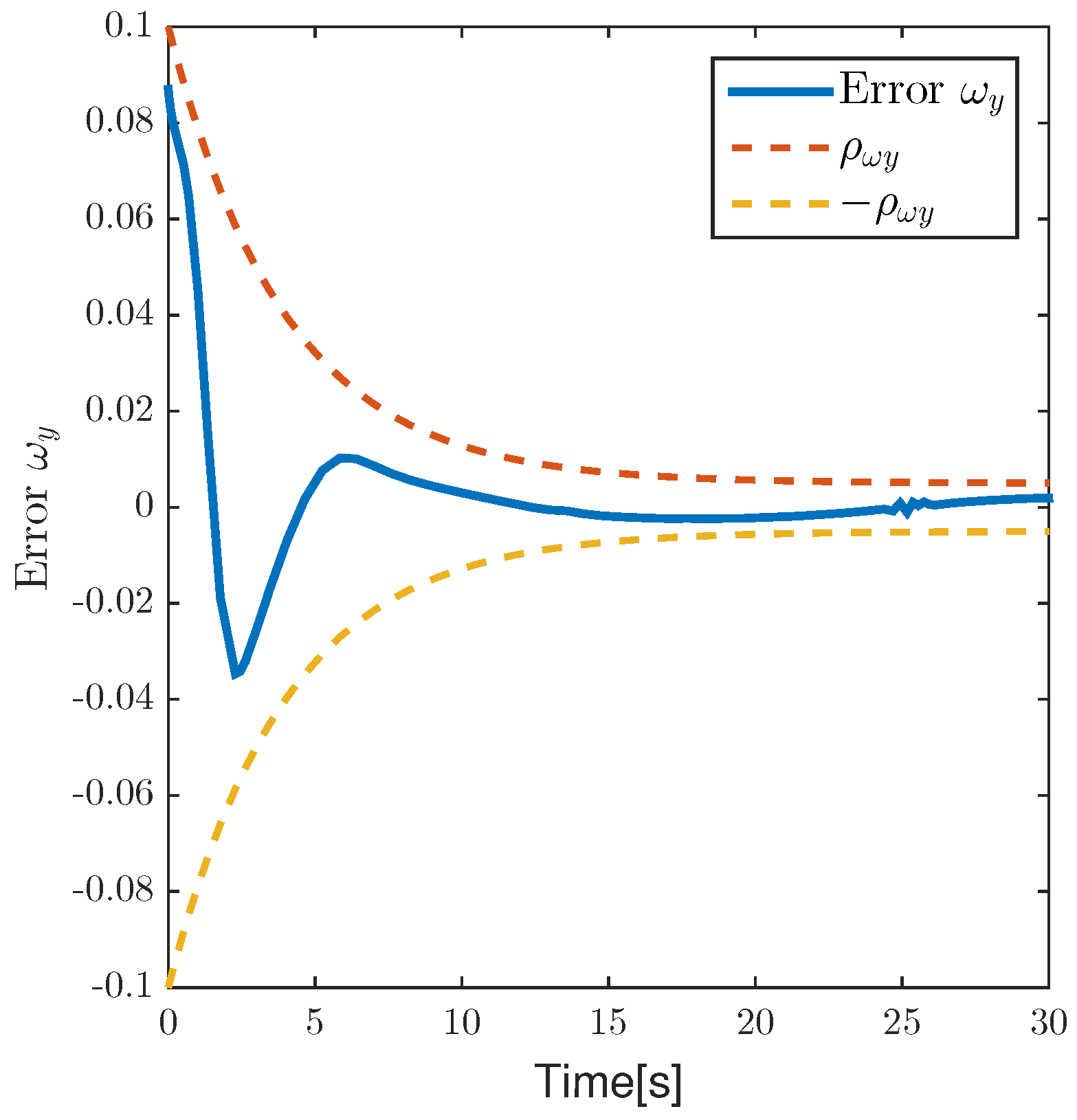
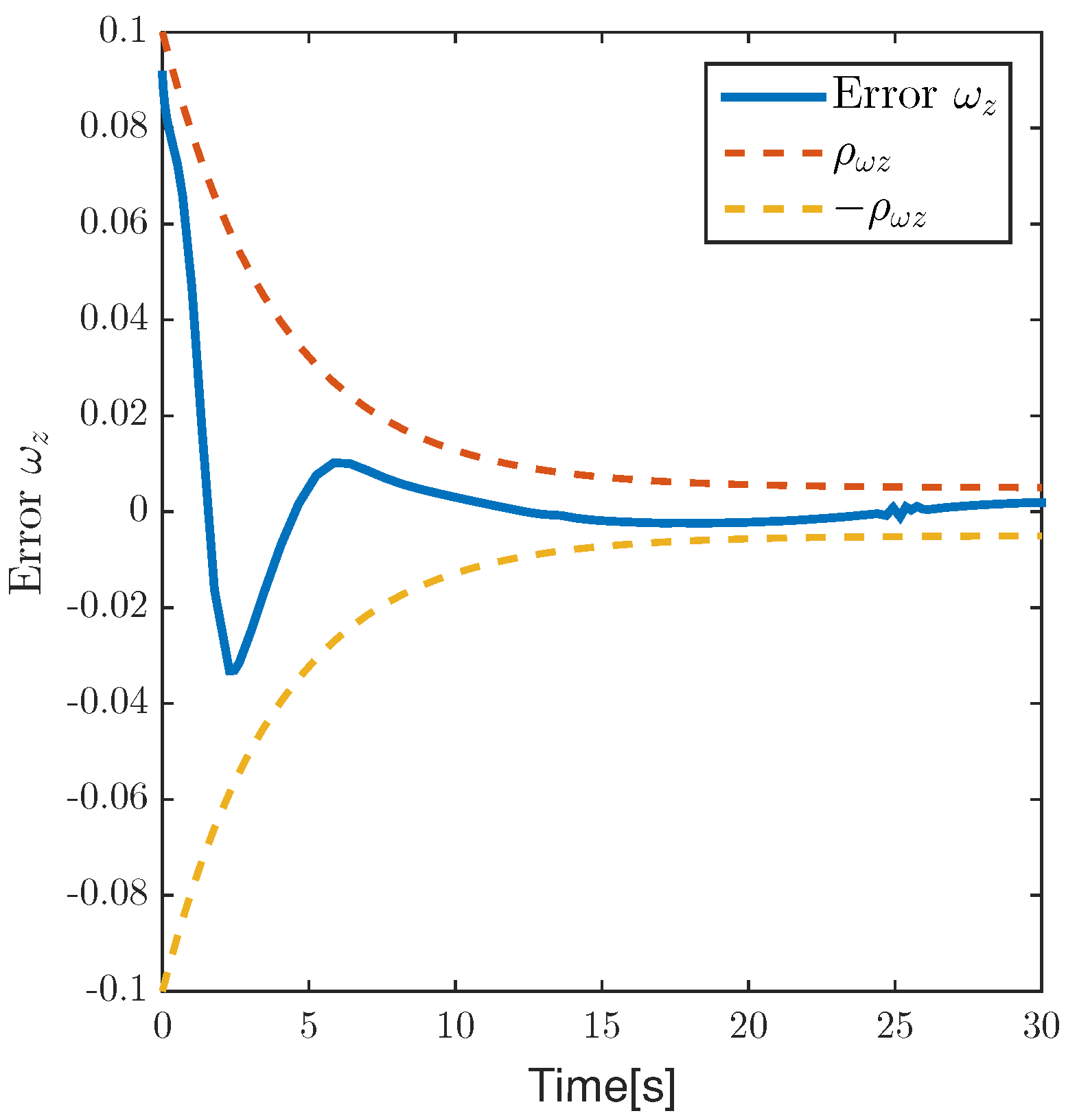
5.2. Simulation Results and Discussion in Asteroid Environment
The target attitude angle is all
, The initial angular velocity of Cubli Rovers is
. The initial attitude angle is set to
,
,
. Gravitational acceleration
, total mass is 2 kg, cube side length is
, The values of performance boundary functions and control parameters in the simulation are shown in the following
Table 2.
The external disturbance values are as follows:
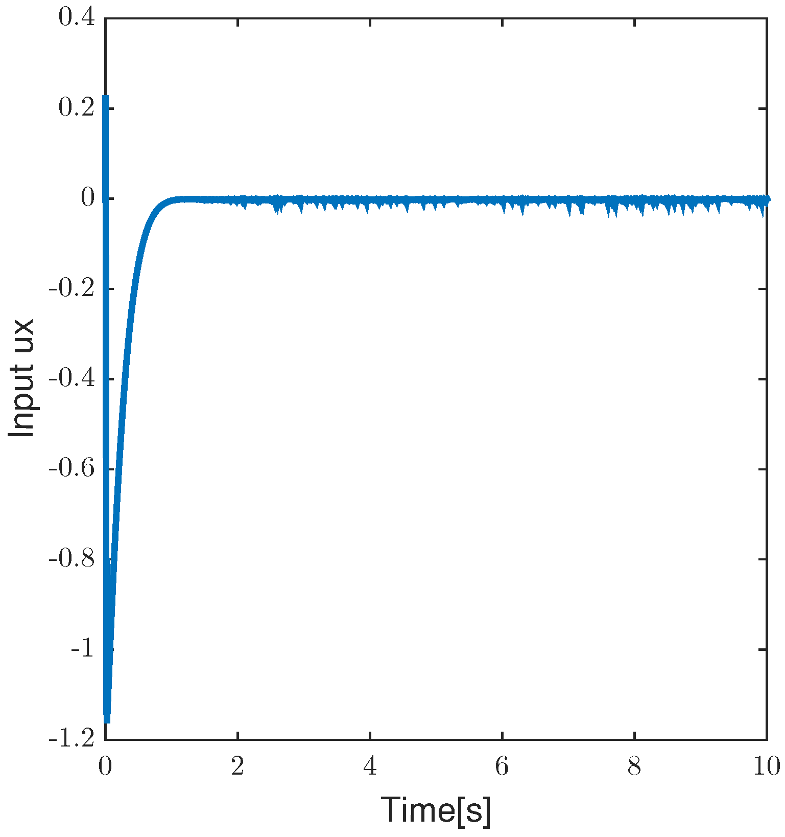
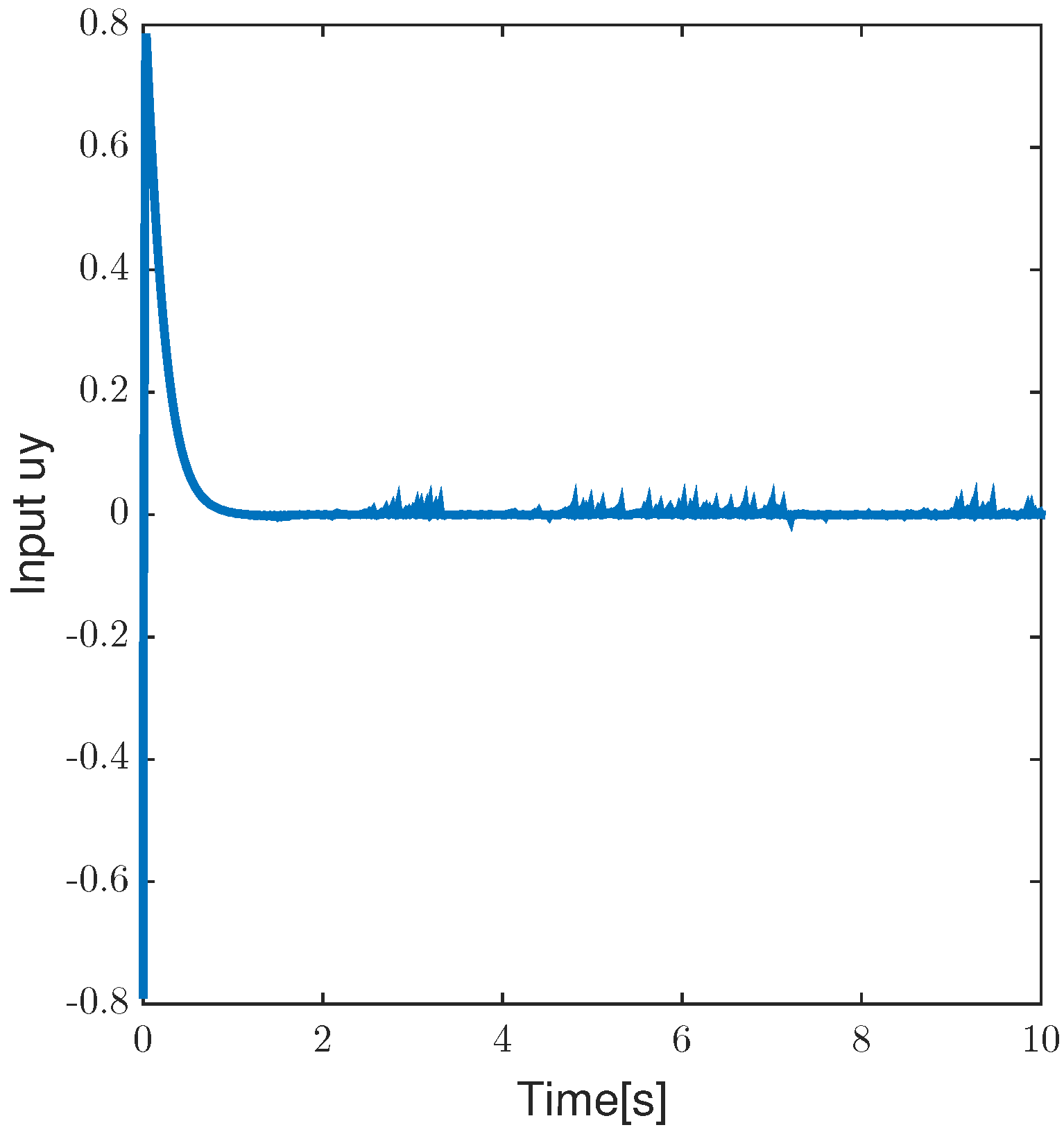
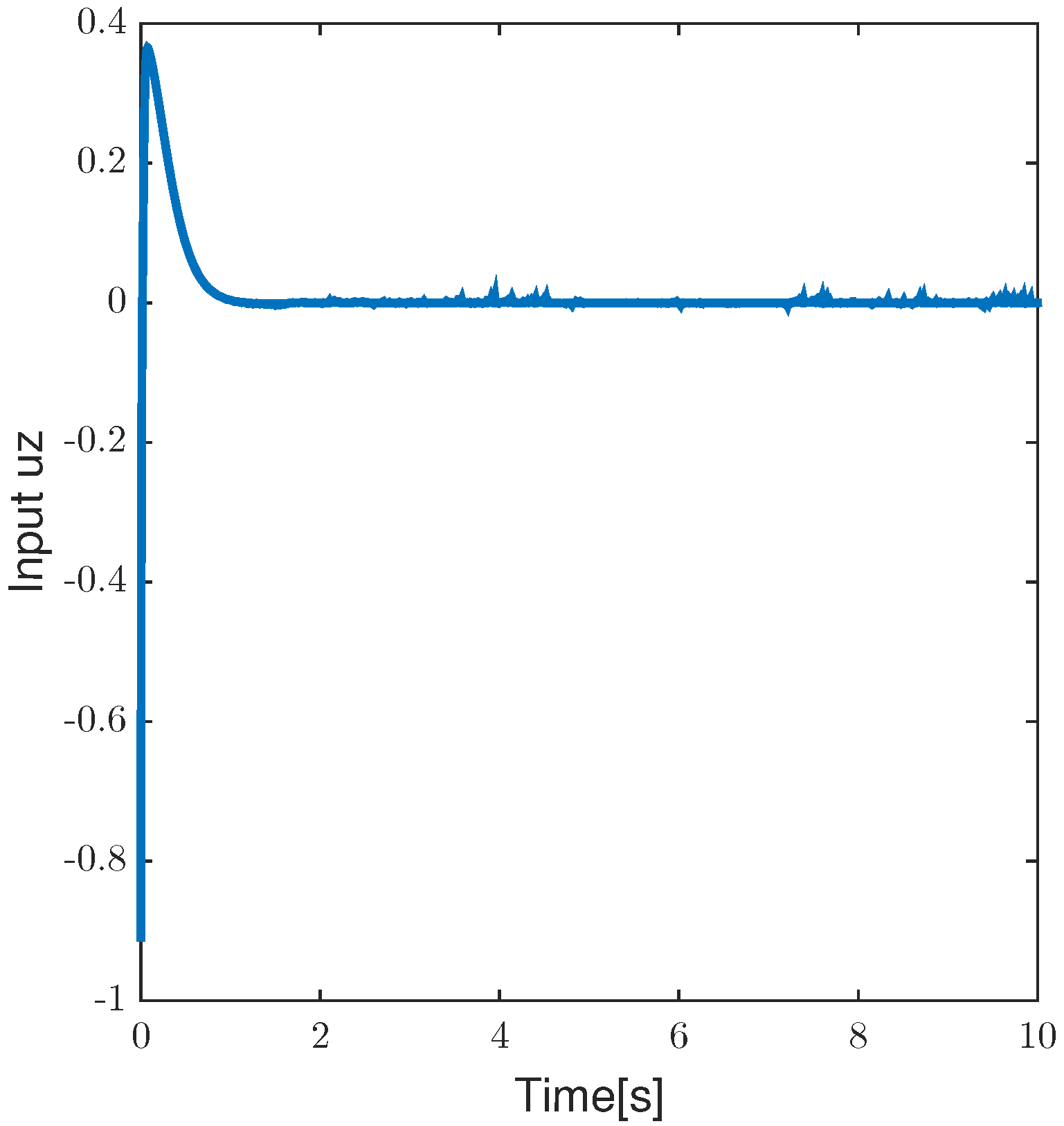
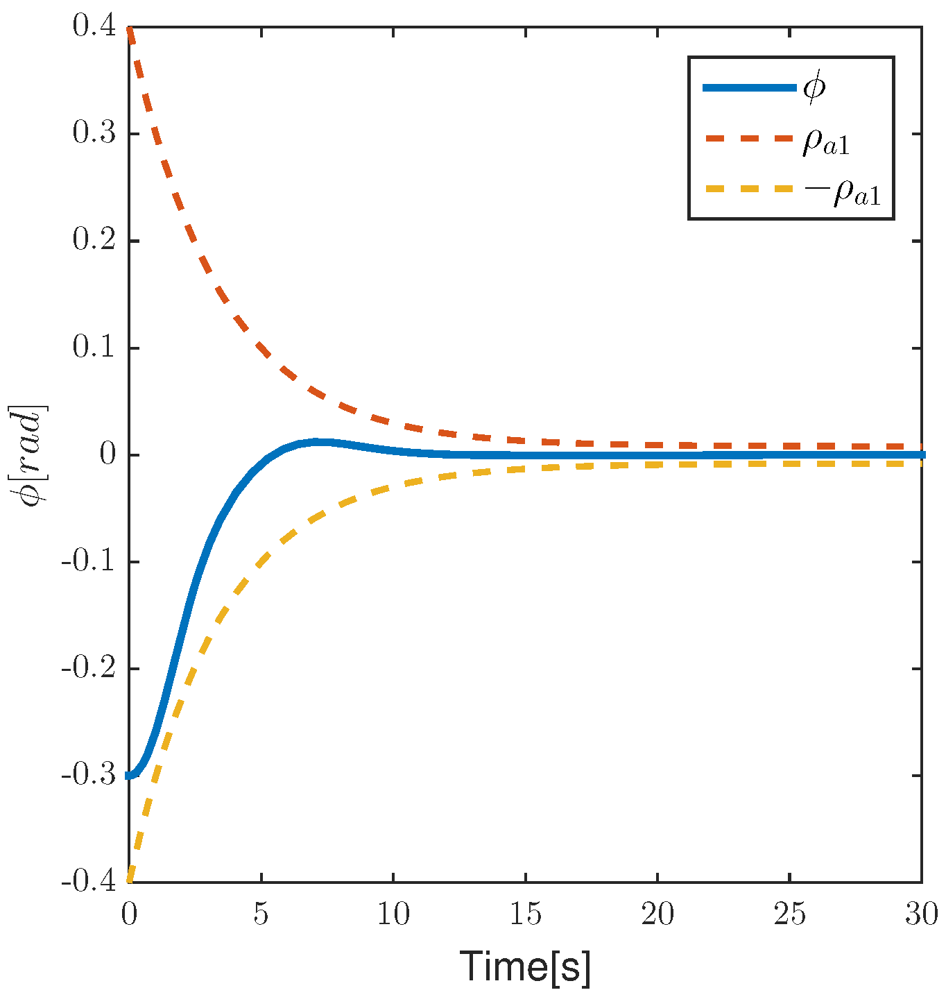
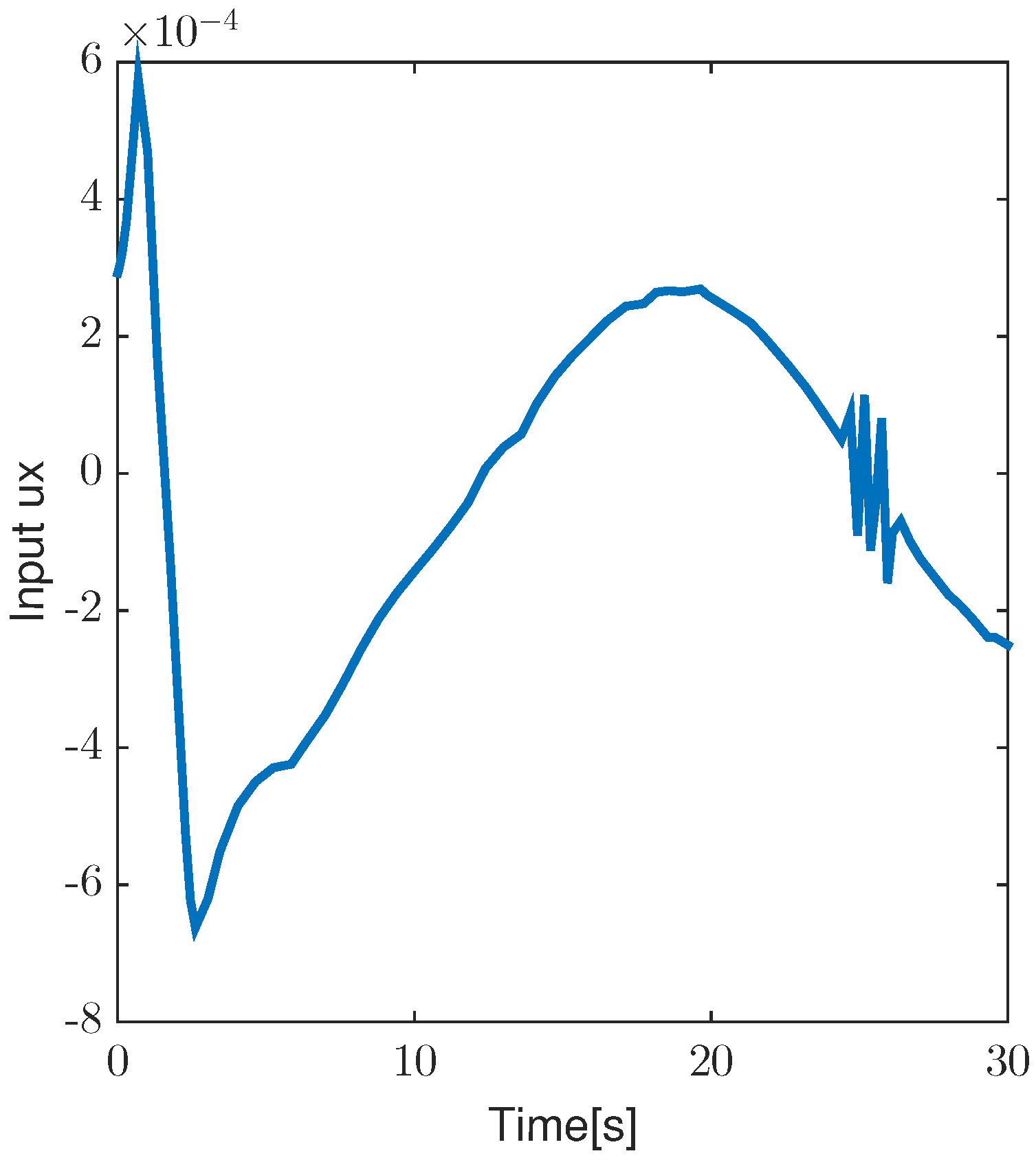
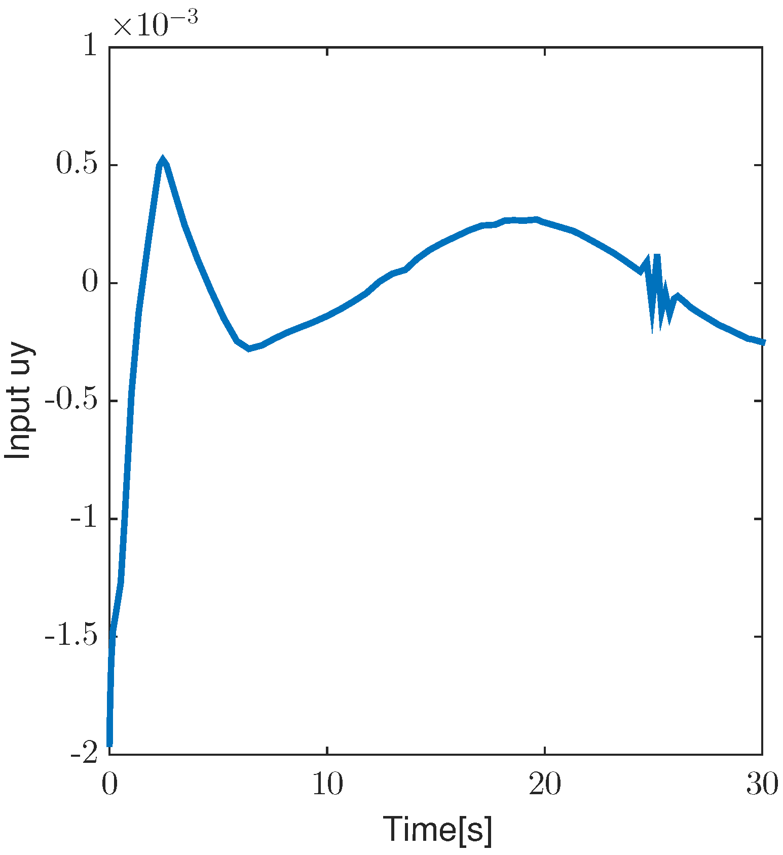
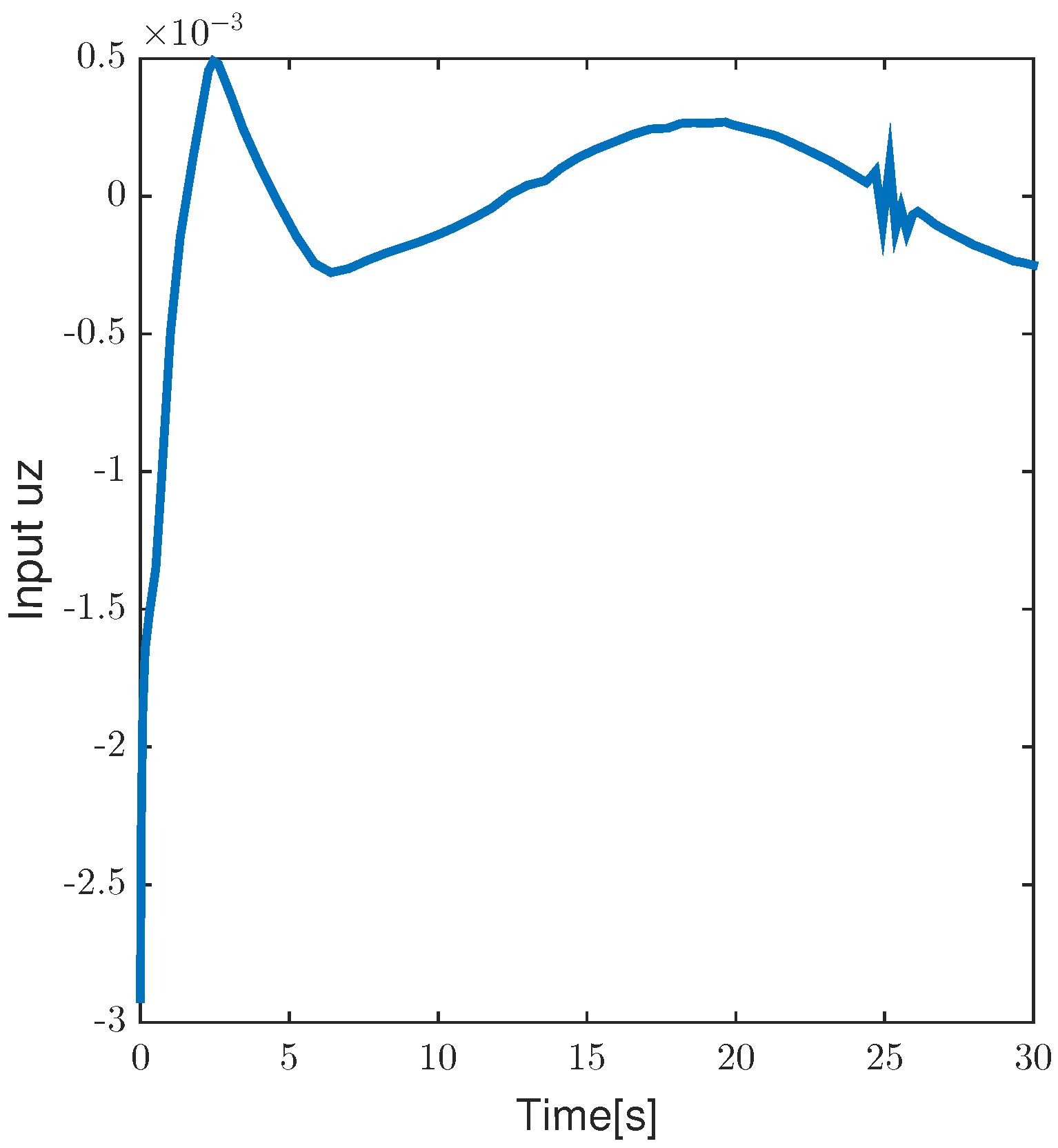
As seen in
Figure 17,
Figure 18,
Figure 19,
Figure 20,
Figure 21,
Figure 22,
Figure 23,
Figure 24,
Figure 25,
Figure 26,
Figure 27 and
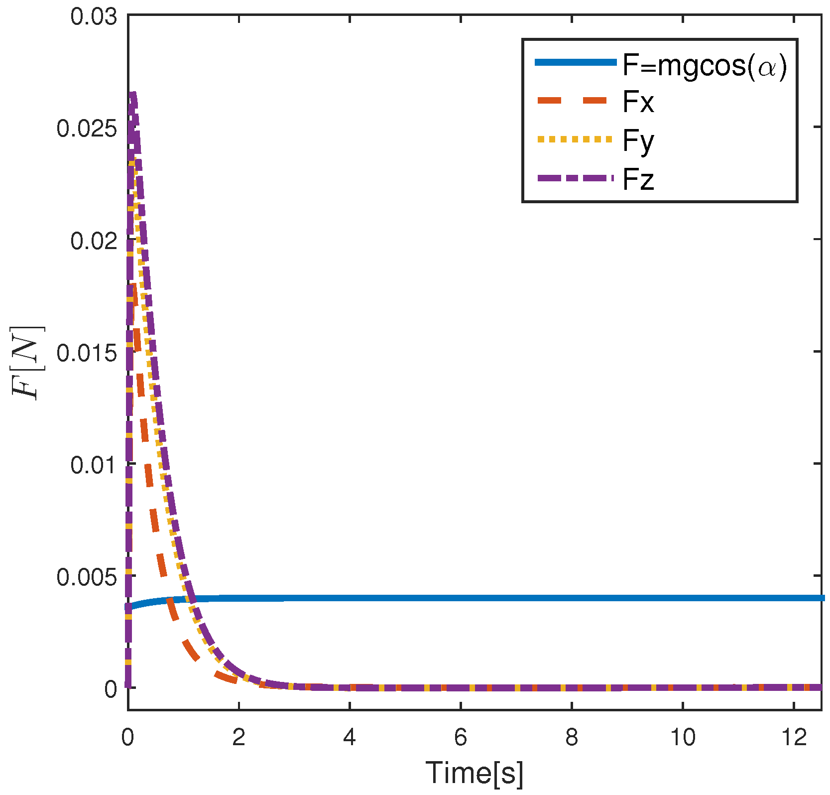
Figure 28, it has been verified by simulation results that it is possible to ensure self-equilibrium stability without leaving the surface of the asteroid through the prescribed performance design. Meanwhile, it can be seen from the figures that in the presence of external disturbances, the control method designed in this paper can well resist external disturbances and ensure that the attitude angle is stable near the steady state. Periodic chattering exists in the input to ensure anti-interference and make the system robust.
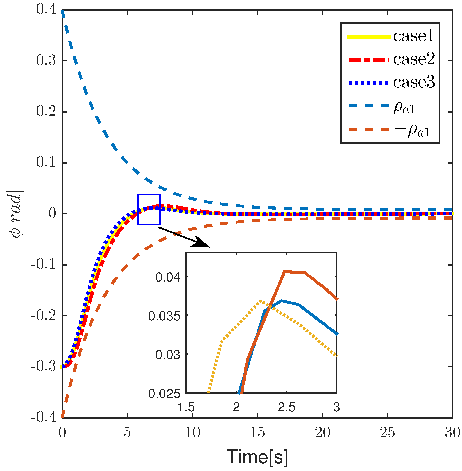
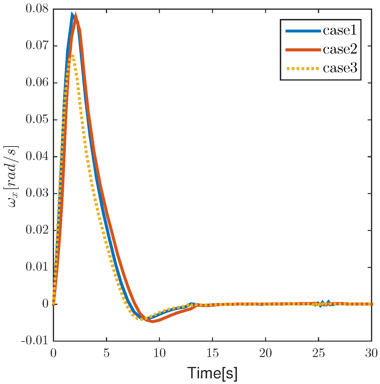
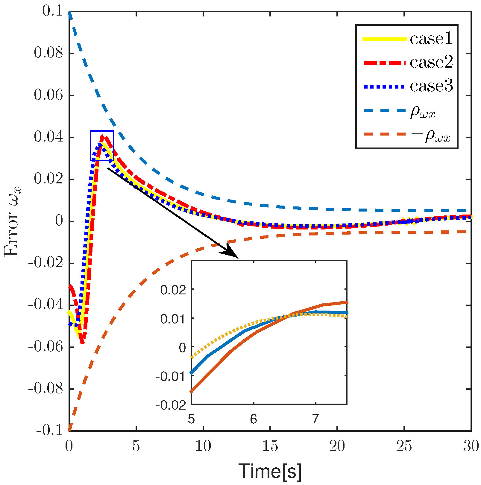
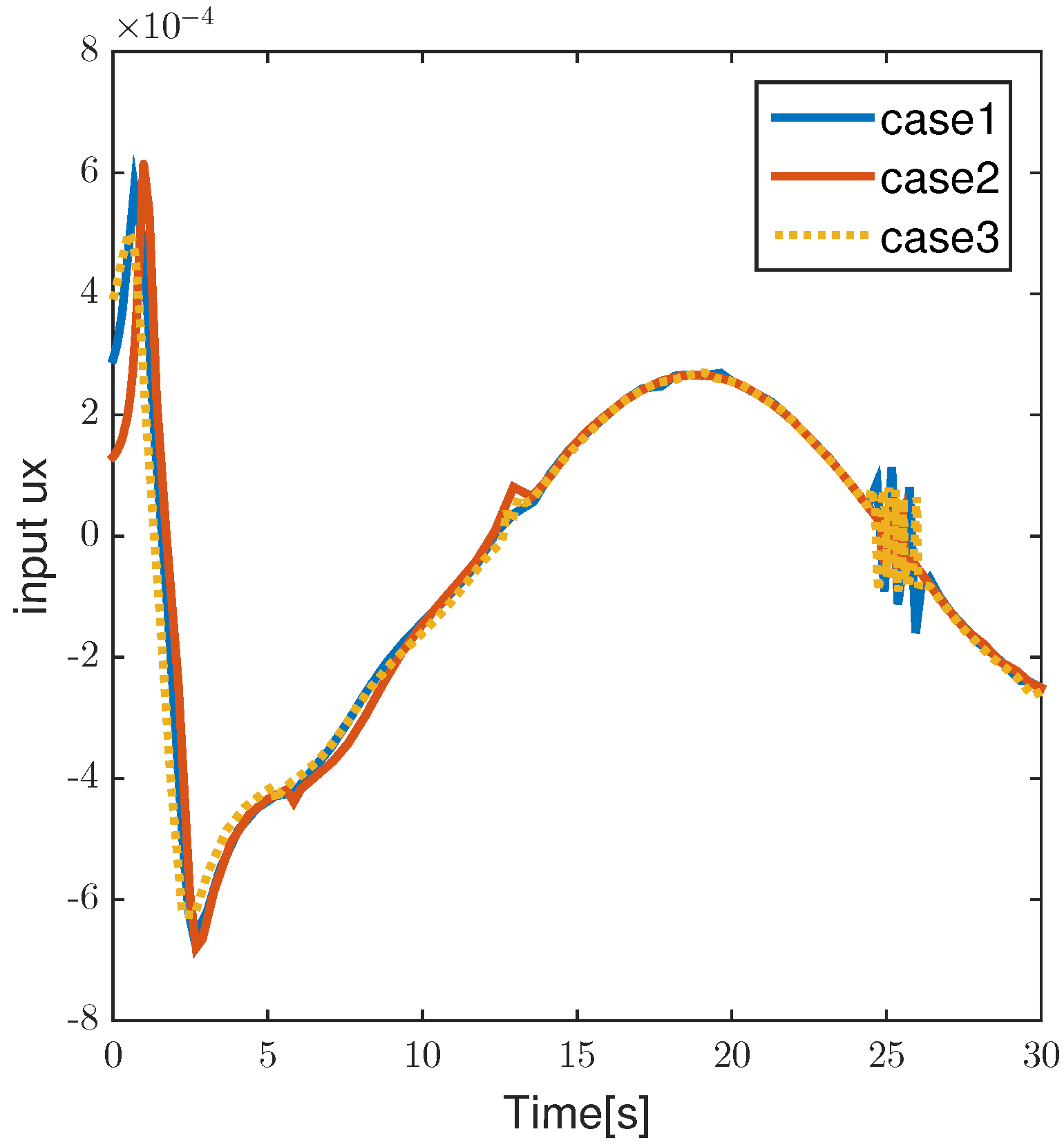
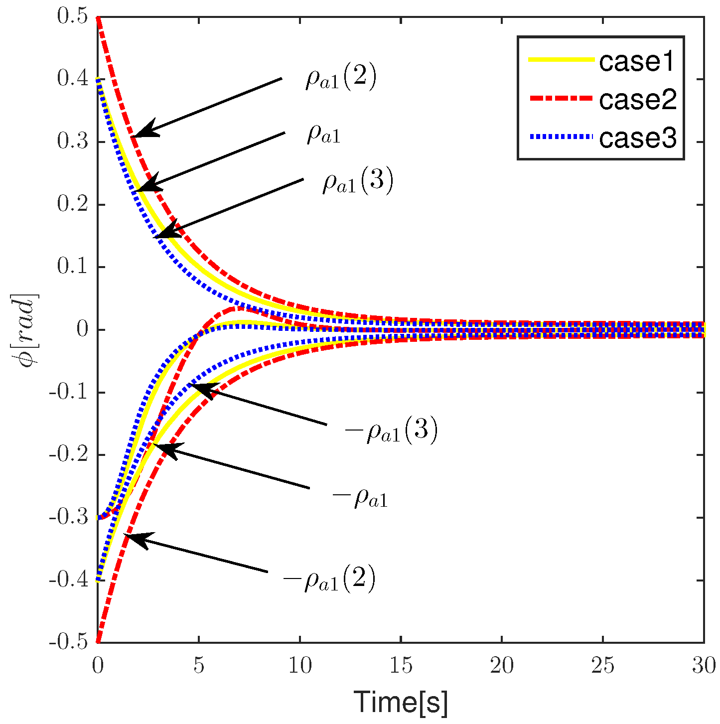
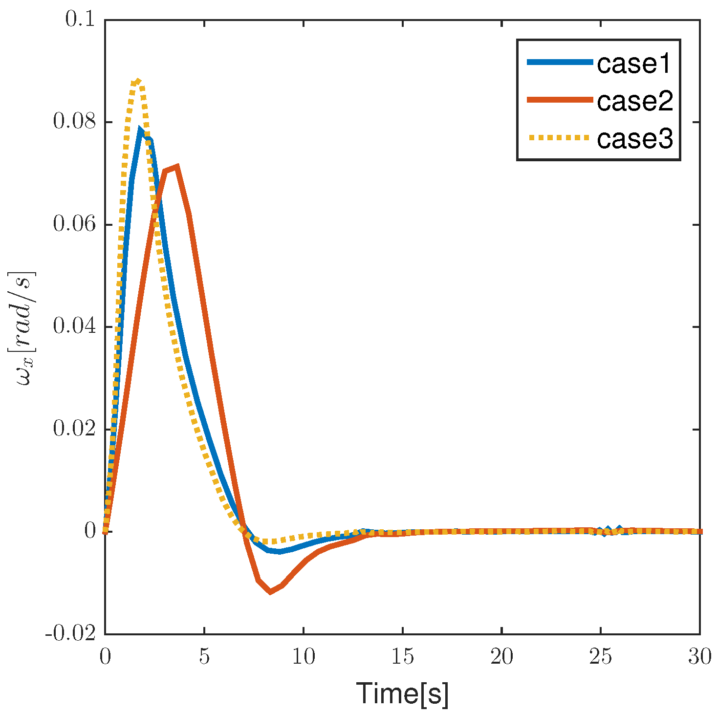
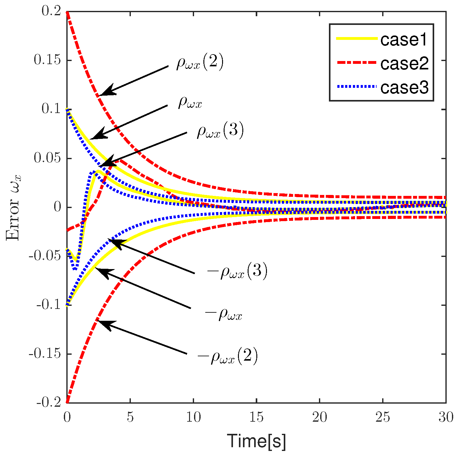
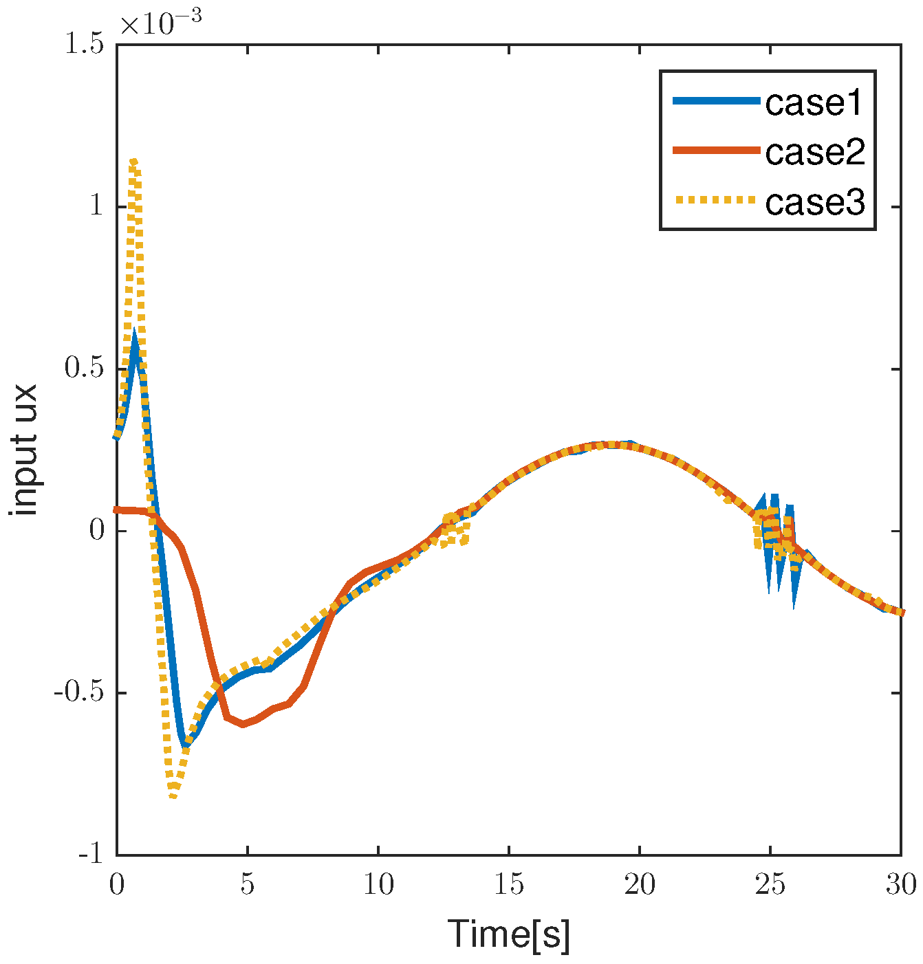
5.3. Performance Comparison Results for Different Control Parameters
(1)
Figure 29,
Figure 30,
Figure 31 and
Figure 32 show that the influence of controller parameters
,
,
. No change in performance boundary function. Three groups of parameters are selected:
Case1: , , , .
Case2: , , .
Case3: , , .
Case1: , , , , ,
Case2: , , , , ,
Case3: , , , , ,
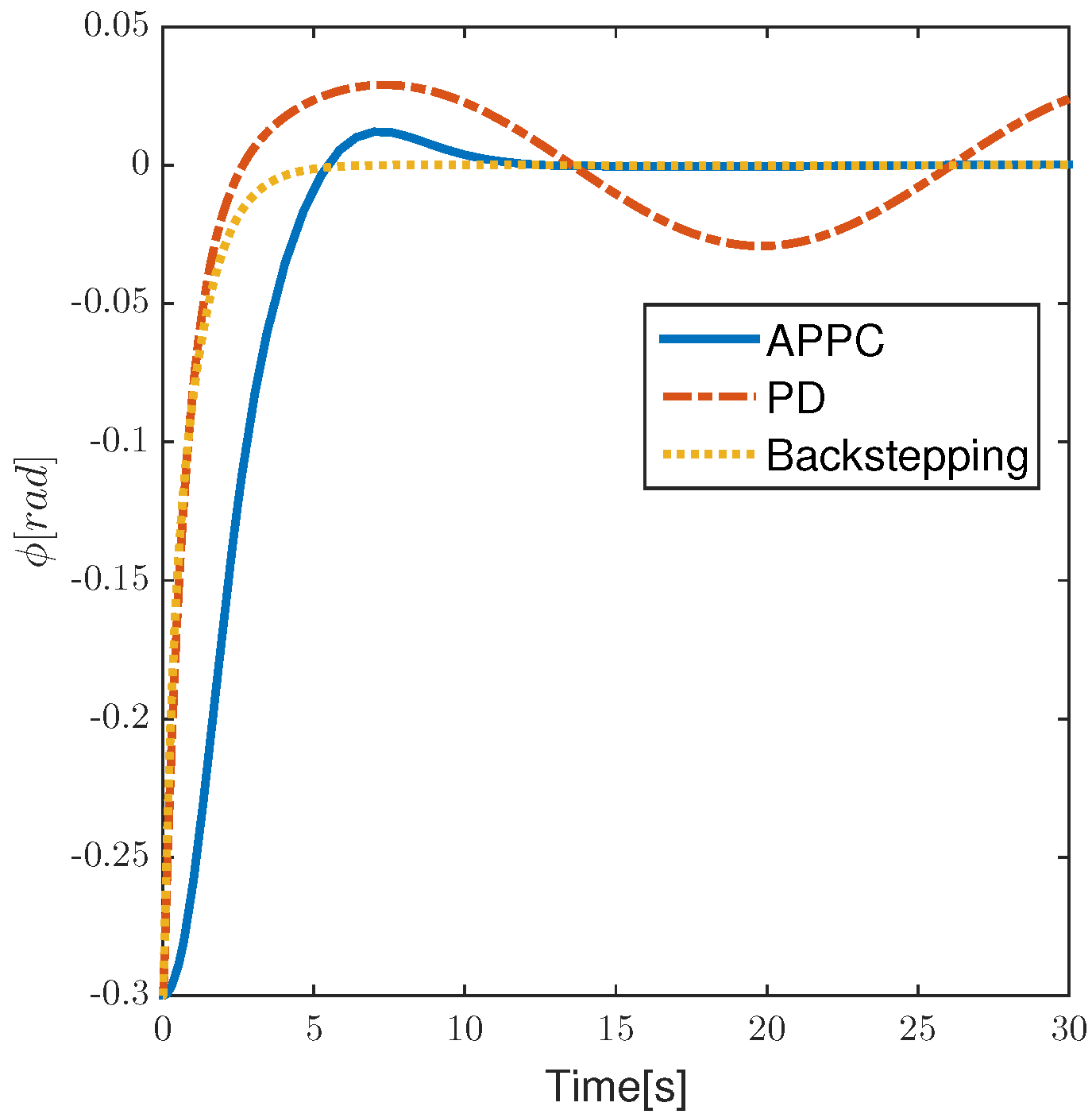
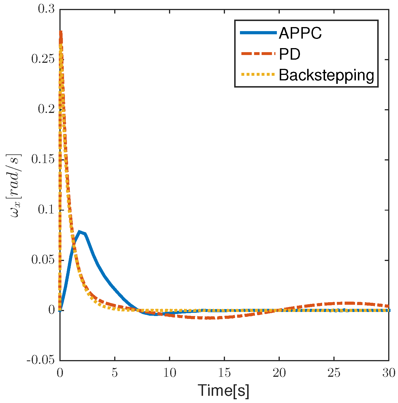
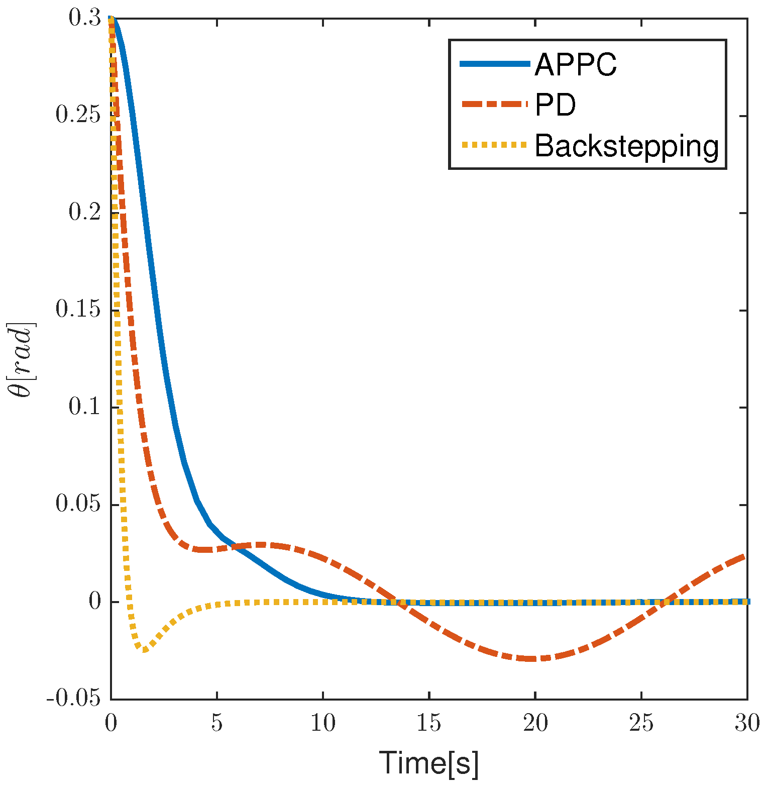
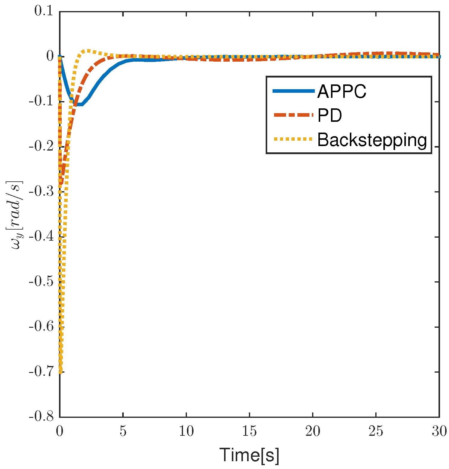
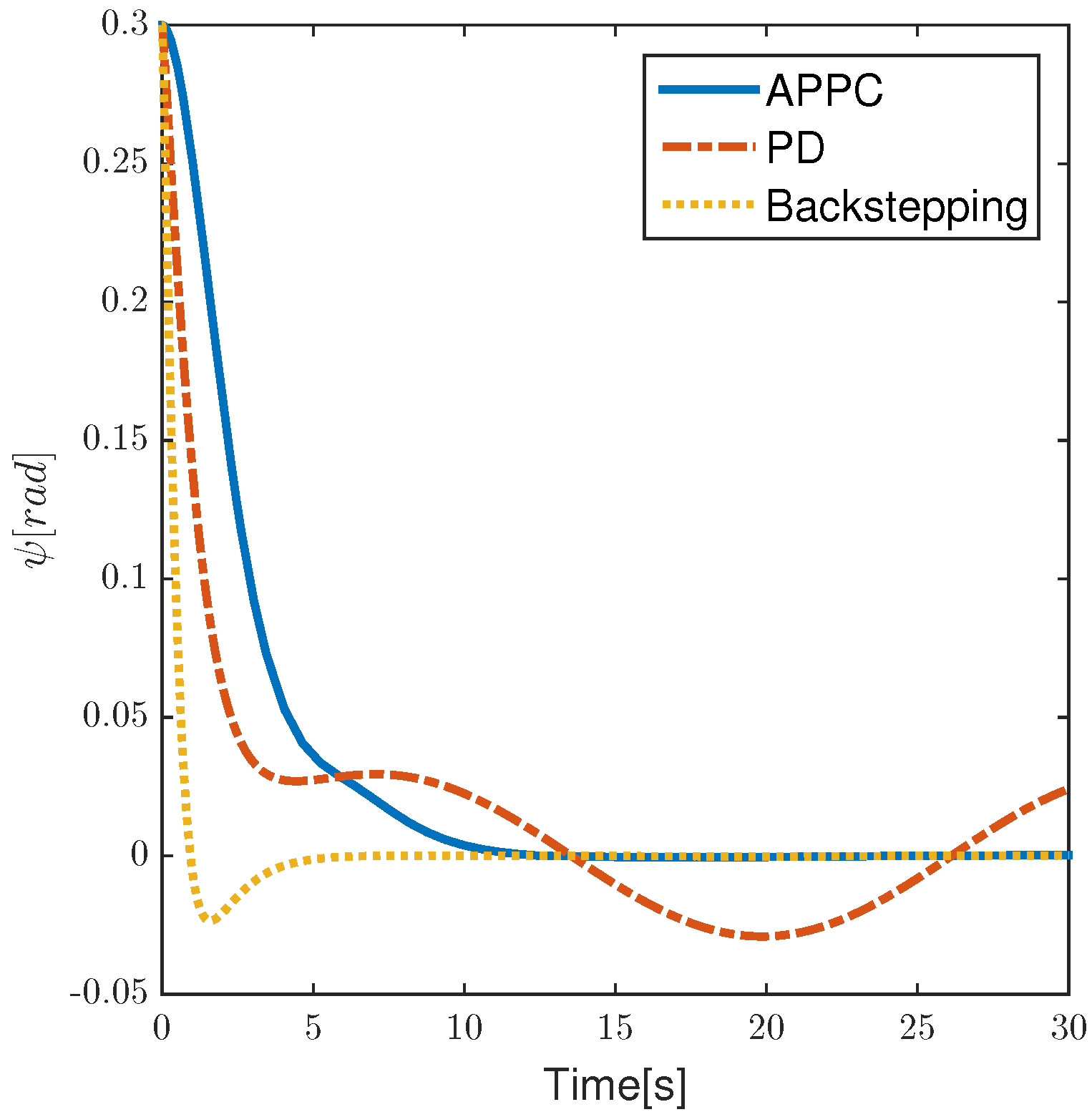
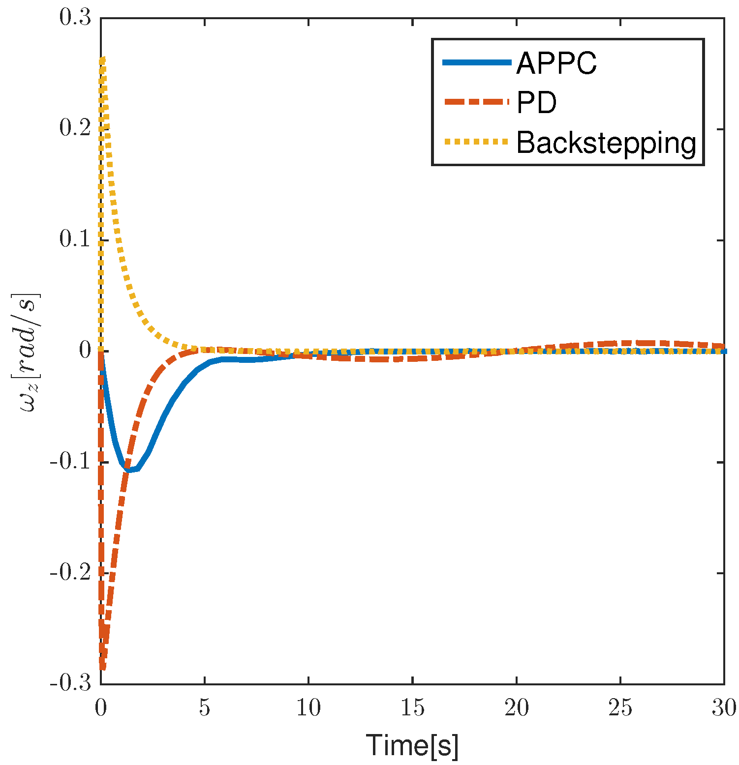
5.4. Comparison Results and Discussion
The method APPC proposed in this paper is compared with the classical PD control and the Backstepping method, and the results are shown in the following
Figure 37,
Figure 38,
Figure 39,
Figure 40,
Figure 41,
Figure 42 and
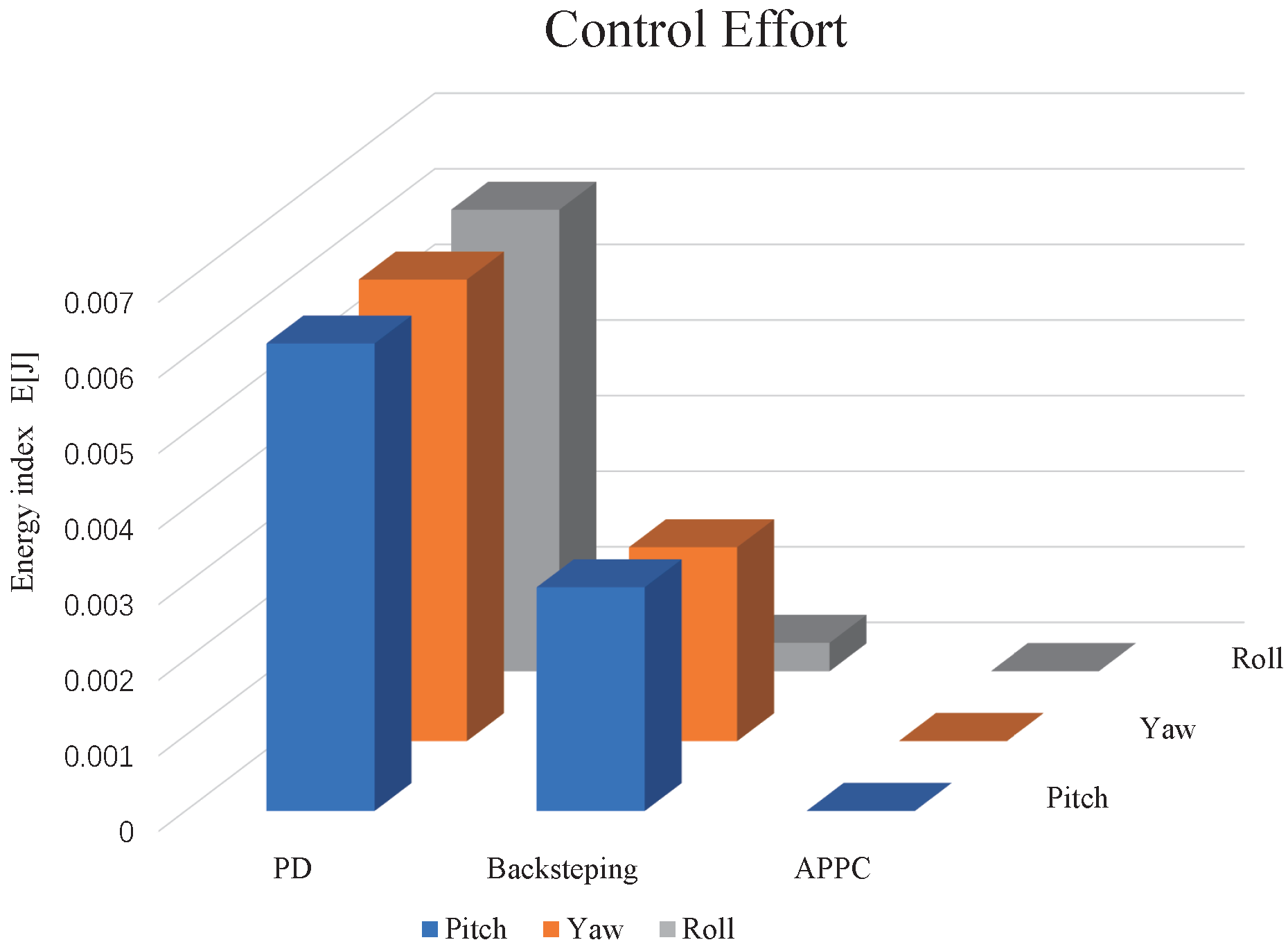
Figure 43. Furthermore, to assess the Control Effort required by different control methods throughout the process, the following indicator is introduced
The following
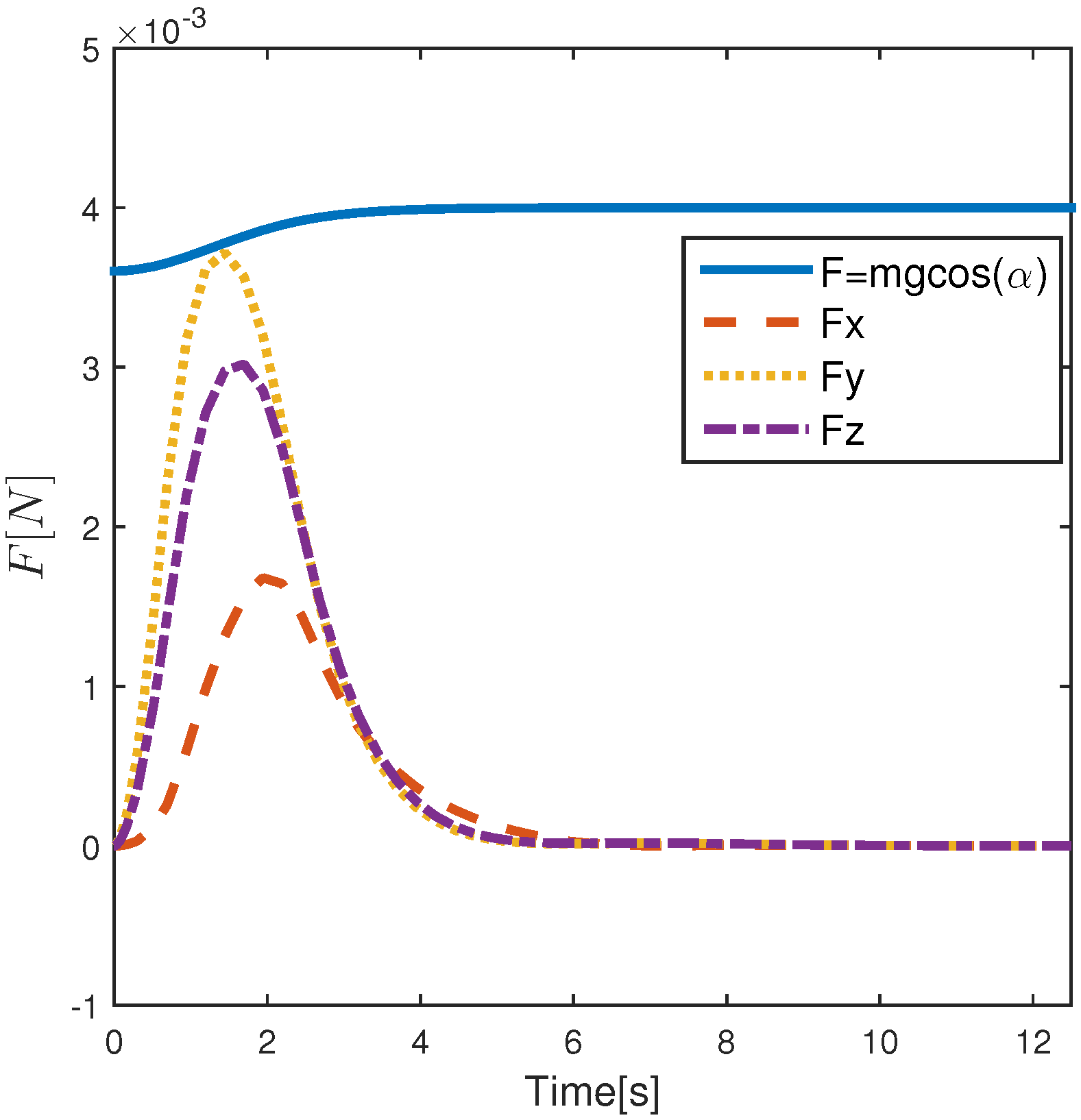
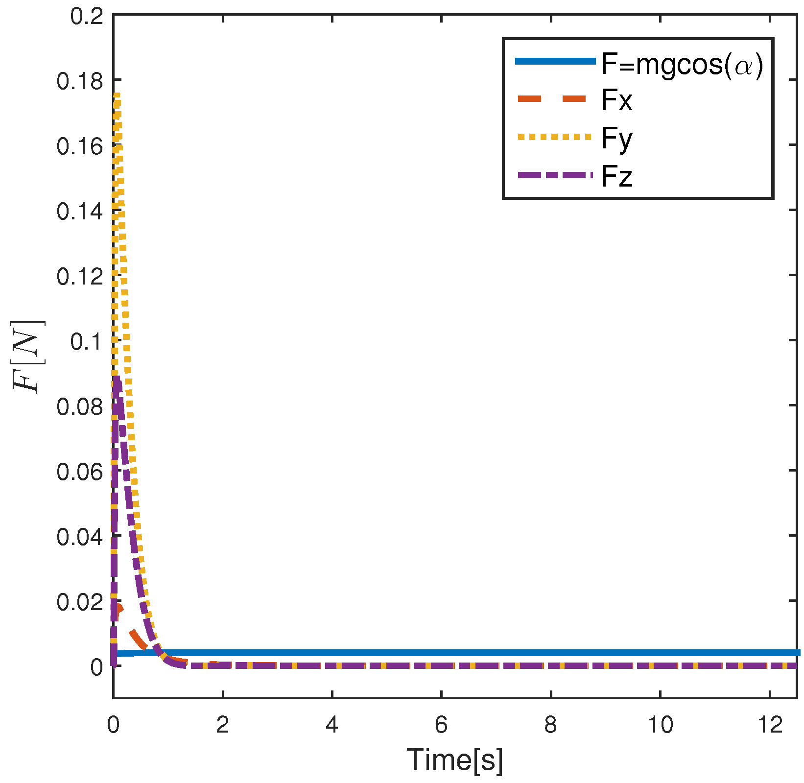
Figure 44,
Figure 45 and
Figure 46 shows the feasibility validation of the three control methods in the case of an asteroid surface:
It can be seen in
Figure 37,
Figure 38,
Figure 39,
Figure 40,
Figure 41 and
Figure 42 that the APPC control method and the Backstepping method [
37] can drive the system to a steady state and have a certain anti-disturbance ability. The system under PD control is greatly affected by disturbance so the state quantity changes periodically around the steady state. As seen in
Figure 43, APPC can well limit the overshoot, and the energy consumed is the smallest in the whole process.
However, it can be seen from
Figure 44,
Figure 45 and
Figure 46 that the speed generated by the Backstepping method and the PD method in the control process has exceeded the tolerance, which makes the Cubli Rovers leave the ground and cannot produce self-balancing stabilization behavior. The APPC method proposed in this paper can ensure the normal movement of the system during the control process by designing the boundary function and limiting convergence rate and overshoot. This is also the advantage of the APPC control method for asteroid surfaces proposed in this paper. The value of angular velocity in the control process of the Backstepping method is too large to satisfy the constraint by verification. Because the control effect of the Backstepping method is better in the need for greater angular velocity input which in turn makes the adjustment time shorter and convergence faster. Of course, control effort is also an important part of the reason. In the asteroidal environment, the Cubli Rovers have no energy source, so energy is limited. Control effort is a concern in order to achieve a larger detection area and a longer operating time.


