Article

An Observer-Based Stiffness Estimation for Space Target Capture by Space Robot with Controllable Damping Mechanism

1
School of Automation, Beijing University of Posts and Telecommunications, Beijing 100876, China
2
Beijing Key Laboratory of Intelligent Space Robotic Systems Technology and Application, Beijing Institute of Spacecraft System Engineering, Beijing 100876, China
*
Author to whom correspondence should be addressed.
Aerospace 2022, 9(11), 726; https://doi.org/10.3390/aerospace9110726
Submission received: 12 October 2022 / Revised: 5 November 2022 / Accepted: 10 November 2022 / Published: 18 November 2022

Abstract

:
The space target capturing task using the spacecraft-manipulator system (SMS) has special significance in on-orbit servicing due to its theoretical challenges and practical value. The contact force between the end effector (gripper) and the target exerted by the tumbling motion of the space target destabilizes the spacecraft base. A full-dimensional controllable damping mechanism (FDCDM) with a cross-axis structure was designed to buffer the transient impact force on the end joint. The introduction of a damping mechanism gives the space robot a variable stiffness and damping system, and a stiffness estimation algorithm is proposed to calibrate the system stiffness, as stiffness cannot be measured directly. The full-dimensional controllable damping mechanism (FDCDM) with a cross-axis structure is equivalent to a four-DOF tandem joint, and the whole-body dynamic model of the SMS endowed with a full-dimensional controllable damping mechanism (FDCDM) was established using the Kane equation. Then, an unknown input observer (UIO)-based identification theory is proposed to precisely estimate the internal flexibility torque and the corresponding joint stiffness. A model-based neural learning algorithm is proposed to update the variable parameter matrix of the observer. The simulation experiment results demonstrate that the flexibility torque and joint stiffness could be accurately estimated within the expected error, illustrating the feasibility and effectiveness of the proposed method.

1. Introduction

On-orbit capture tasks performed by space robots mainly include removing space debris, disposing of failed satellites, and so on [1,2,3,4]. These robots can not only clean up the space environment, but also repair and recover failed satellites, reducing the potential hidden dangers to orbiting spacecraft [5]. Therefore, grasping and manipulating uncooperative space targets are emerging challenges for space robots. Hand-like opposed grippers are widely used as end effectors to interact with the target, which essentially employ rigid contact so that a large impact force can be exerted. Therefore, developing new soft-docking mechanisms for grippers to buffer impact energy is an urgent demand for capture tasks.
To solve this problem, various end effectors for grippers have been studied. Space net capture is an effective method for the removal of tumbling debris that provides a prospective viewpoint for the capture of large, noncooperative space objects [6,7,8,9,10]. A reduced multiobjective optimization framework has been presented using a lumped parameter modeling method to solve the space net design problem. A net capture dynamic was established in [11] to simulate the movements of a flexible net that can be opened or closed repeatedly. Other mechanical-based end effectors have also been widely researched. In [12], a novel capture mechanism endowed with a series of hollow-shaped end effectors for a dual-arm space robot was designed to cage the non-graspable targets. In order to capture a wide range of target objects with various sizes and shapes, an articulated arm consisting of a series of jointed segments with different lengths was designed in [13], which is driven by two motors pulling on a Kevlar cord. Recently, variable-stiffness actuators (VSAs) and variable damping mechanisms have received extensive attention due to their advantages in terms of compliant operation and softer contact [14,15,16]. A self-learning, soft-grasp control algorithm for a variable stiffness joint was proposed to minimize the base angular momentum in [17]. Using damping force to buffer the collision is also an effective active control method. The magnetorheological (MR) damper is widely used because of its characteristics of controllability and fast response through vibration control [18]. In [19], a controllable damper mechanism using an MR damper was proposed to dampen the angular momentum of the spinning target and stabilize the base without knowledge of manipulator or target dynamics. In [20], a control strategy for a rehabilitation robot using an MR damper to protect the machine mechanism from vibration in one of the horizontal directions was presented. The employment of variable stiffness and variable damping provides a prospective method for the capture of noncooperative space targets. However, the relevant research is limited to one-direction damping forces and the accurate modeling of the whole-body dynamics.
The introduction of a variable damping mechanism increases the difficulty of modeling due to the flexible forces involved. In the early years, many studies focused on multilink flexible robots consisting entirely of revolute joints [21,22,23]. However, these studies mainly focused on the use of the assumed modes method (AMM) for dynamic modeling. The authors of [24] considered the unmodeled dynamics and dead zone of the flexible-joint manipulator and proposed an equivalent-input-disturbance (EID) method for the tracking control. The nonlinear vibration of a two-link flexible manipulator was discussed and an effective vibration absorber was implemented based on the internal resonance relationship in [25]. In [26], a bisection method-based algorithm was proposed to analyze the inverse dynamic responses of a flexible robot sliding through a prismatic joint. The extended-state observer (ESO) was used to achieve improved model compensation without velocity measurement in [27,28]. A whole-body dynamic model of a nonholonomic mobile manipulator with series elastic actuators (SEAs) was proposed under the uncertainties of the flexible-joint robot model in [29]. Though there have been many studies focused on the dynamic modeling of different kinds of specific flexible robots, little attention has been paid to the active controllable flexible force in the dynamic equations outputted by SEAs and the controllable damping mechanism.
The introduction of joint flexibility not only makes the dynamics model more complicated, but also increases the parameter uncertainty of the system as a result of the VSAs, SEAs, and variable damping mechanism. However, since it is impractical to measure the joint stiffness directly, the development of a parameter identification and stiffness estimation approach to compensate for the model errors is an urgent challenge to be solved. The theoretical idea is to obtain the stiffness from the first derivative of the flexibility torque with respect to the deflection angle. In [30], time-varying stiffness was estimated through a force function reconstructed using a polynomial expansion. An intelligent variable-stiffness actuator and a new stiffness estimation method without torque feedback were developed in [31]. The authors of [32] considered the problem of estimating the nonlinear stiffness of VSAs with an algorithm based on modulating functions to avoid the need for a numerical derivative. In [33], the stiffness estimation problem for flexible robot joints with VSAs is dealt with by considering the flexibility torque as an unknown signal, and an unknown input observer theory is proposed. In [34], a nonlinear observer and a reduced parametric model are presented for online stiffness estimation. Summarizing from the above studies, stiffness estimation usually takes two steps: first, an estimate of the flexibility torque applied to each motor is obtained by utilizing the nonlinear model of the flexibility torque; then, the recursive least square (RLS) algorithm is applied to estimate the unknown parameters, and the stiffness is derived from the identified approximation model. In summary, the main contributions of this paper are as follows:
(1)
A controllable damping mechanism with a cross-axis structure is introduced into the end joint of the space robot, and the whole-body dynamic model is established by using the Kane method.
(2)
A stiffness estimation approach based on an unknown input observer (UIO) is proposed to estimate the flexible force of the flexible robot with a controllable damping mechanism. Additionally, the global asymptotic stability of the estimation approach is guaranteed by using the Lyapunov theory.
(3)
A neural learning algorithm is developed to update the variable parameter matrix of the estimation approach, and a recursive least square (RLS) algorithm is applied to estimate the stiffness of the system.
(4)
The results of the numerical simulation experiments in MATLAB demonstrate superior performance in terms of stiffness estimation accuracy without a force sensor.

2. Modeling of Spacecraft-Manipulator System with FDCDM

The full-dimensional controllable damping mechanism (FDCDM) with four DOFs is shown in Figure 1. In this paper, the spacecraft-manipulator system is composed of a spatial base with six DOFs and a manipulator with two DOFs. The FDCDM consists of a cross-axis structure with three rotary dampers and a sliding structure with one linear damper. The exploded drawing is shown in Figure 2.
As shown in Figure 1 and Figure 2, the controllable damping mechanism with a cross-axis structure has four DOFs: a rotary x axis; a rotary y axis; a rotary z axis to output the spatial three-dimensional damping torque around the x axis, y axis, and z axis, respectively; and a sliding z axis to output a linear damping force along the z axis. As shown in Figure 3, the linear contact force F X along the x axis can be converted into a torque M Y 2 around the rotary y axis. Similarly, the linear contact force F Y along the y axis can be converted into a torque M X 2 around the rotary x axis. In other words, the flexible rotating damping torque of the rotary x axis and rotary-y axis can indirectly buffer the contact force along the y axis and x axis to realize the buffering and unloading of the spatial six-dimensional contact force.

2.1. Equivalent Kinematics Equation

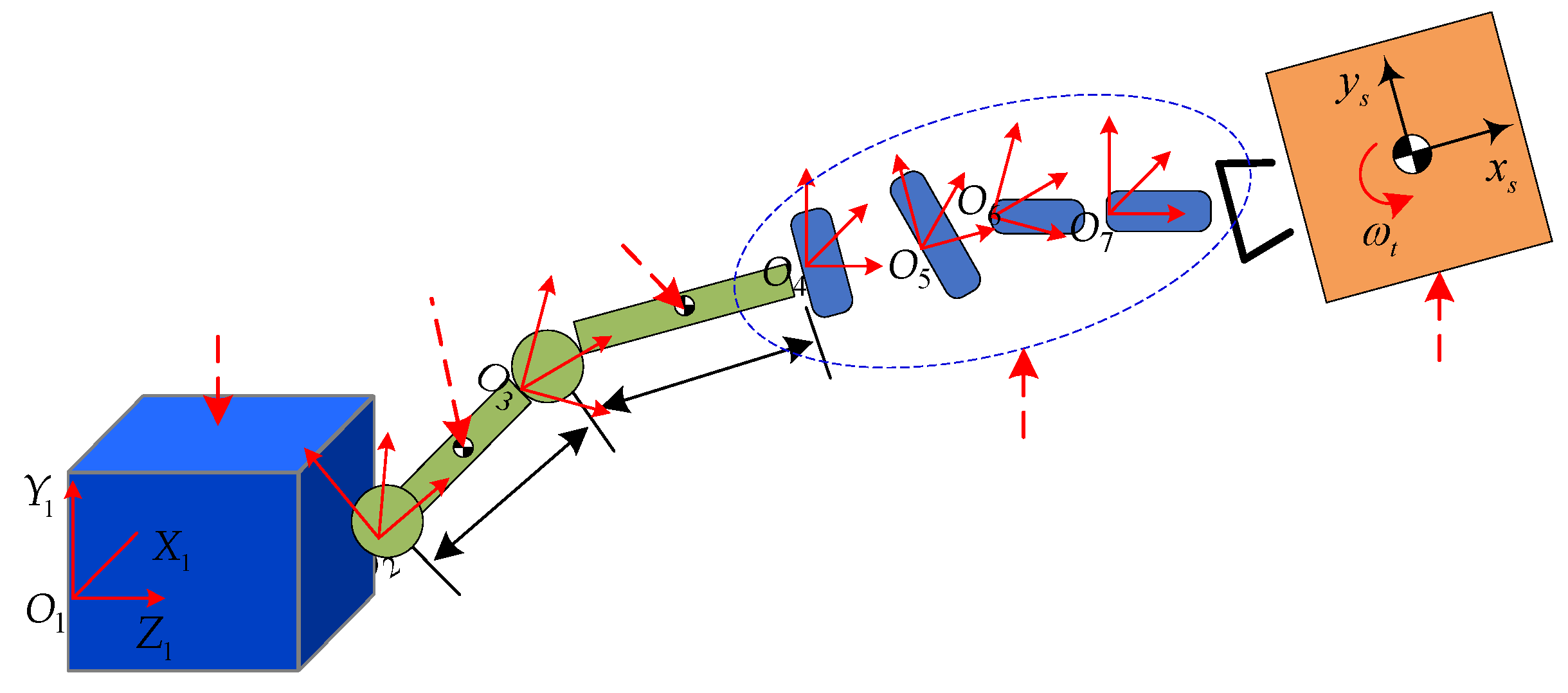
The full-dimensional damping force of the FDCDM can be equivalent to the actuator outputs in the end joint, as shown in Figure 4 and Figure 5.
The relative linear velocities and angular velocities between the adjacent rigid bodies k and k−1 are set as v k k 1 and ω k k 1 (k = 1, 2, 3, …, 7), respectively. Additionally, the relative line displacement and angular displacement are set as s k k 1 and q k k 1 , respectively. We have
q 1 0 = [ β 1   β 2   β 3 ] T       ω 1 0 = [ α 1   α 2   α 3 ] T q 2 1 = [ 0   0   β 4 ] T               ω 2 1 = [ 0   0   α 4 ] T q 3 2 = [ β 5   0   0 ] T               ω 3 2 = [ α 5   0   0 ] T q 4 3 = [ β 6   0   0 ] T               ω 4 3 = [ α 6   0   0 ] T q 5 4 = [ 0   β 7   0 ] T               ω 5 4 = [ 0   α 7   0 ] T q 6 5 = [ 0   0   β 8 ] T               ω 6 5 = [ 0   0   α 8 ] T s 1 0 = [ β 9   β 10   β 11 ] T       v 1 0 = [ α 9   α 10   α 11 ] T s 7 6 = [ 0   0   β 12 ] T                   v 7 6 = [ 0   0   α 12 ] T s 2 1 = s 3 2 = s 4 3 = s 5 4 = s 6 5 = [ 0   0   0 ] T v 2 1 = v 3 2 = v 4 3 = v 5 4 = v 6 5 = [ 0   0   0 ] T
where α 12 × 1 denotes the generalized velocity and β 12 × 1 denotes the generalized position.
Then, we can obtain the relative rotation matrix of the proprio-coordinate system in rigid bodies k and (k−1), set as A k k 1 3 × 3 :
A 0 1 = Rot ( X , β 1 ) Rot ( Y , β 2 ) Rot ( Z , β 3 ) A 2 1 = Rot ( Z , β 4 ) , A 3 2 = Rot ( X , β 5 ) A 4 3 = Rot ( X , β 6 ) , A 5 4 = Rot ( Y , β 7 ) A 6 5 = Rot ( Z , β 8 ) , A 7 6 = I
Σ k is the ontology coordinate system in rigid bodies k, and Σ 0 denotes the inertial coordinate system; then, the absolute rotation matrix of Σ k and Σ 0 is
A k 0 = A 1 0 A 2 1 A k k 1
In this paper, the base proprio-coordinate system Σ 1 is XYZ Euler angles γ relative to the inertial coordinate system Σ 0 , denoted as γ = [ β 1 β 2 β 3 ] T . Then, the angular velocity of the base in the inertial frame ω 1 0 is
ω 1 0 = [ β ˙ 1 0 0 ] + Rot ( X , β 1 ) [ 0 β ˙ 2 0 ] + Rot ( X , β 1 ) Rot ( Y , β 2 ) [ 0 0 β ˙ 3 ]
Further, the kinematic equation of the model is
β ˙ = D α
where
D = [ H 3 × 3 O 3 × 9 O 9 × 3 I 9 × 9 ] 12 × 12 ,   H 3 × 3 = 1 c β 2 [ c β 2 s β 1 s β 2 c β 1 s β 2 0 c β 1 c β 2 s β 1 c β 2 0 s β 1 c β 1 ] .
where c β denotes cos β and s β denotes sin β .
Let x 12 × 12 replace β , and y 12 × 12 replace α ; thus, the kinematic equation of the system is
x ˙ = D y

2.2. Partial Velocity Equation

The angular velocity of bodies k in the inertial coordinate system Σ 0 is written as:
ω k 0 = ω 1 0 + i = 1 k 1 A i 0 ω i + 1 i
The partial angular velocity is defined as
ω k l = ω k 0 y l l = 1 , 2 , 3 , , 12
Substituting Equation (7) into (8), we can obtain the partial angular velocity W 21 × 12 as
W = [ I 3 × 3 O 3 × 1 O 3 × 1 O 3 × 1 O 3 × 1 O 3 × 1 O 3 × 4 I 3 × 3 A 13 0 O 3 × 1 O 3 × 1 O 3 × 1 O 3 × 1 O 3 × 4 I 3 × 3 A 13 0 A 21 0 O 3 × 1 O 3 × 1 O 3 × 1 O 3 × 4 I 3 × 3 A 13 0 A 21 0 A 31 0 O 3 × 1 O 3 × 1 O 3 × 4 I 3 × 3 A 13 0 A 21 0 A 31 0 A 42 0 O 3 × 1 O 3 × 4 I 3 × 3 A 13 0 A 21 0 A 31 0 A 42 0 A 53 0 O 3 × 4 I 3 × 3 A 13 0 A 21 0 A 31 0 A 42 0 A 53 0 O 3 × 4 ]
where A i j 0 3 × 1 is the jth column of A i o , I 3 × 3 represents the identity matrix of 3 × 3 , and O 3 × 1 denotes the zero vector of 3 × 1 .
The position vector of the mass center of the rigid body k in the inertial frame Σ 0 is
p k 0 = s 1 0 + i = 1 k 1 A i 0 ( d i + s i + 1 i ) + A k 0 r k
where d i denotes the position vector of the rigid bodies k in the coordinate system Σ i , and r k represents the centroid position vector of the rigid bodies k in the coordinate system Σ k .
Differentiating p k 0 in Equation (10) with respect to time, we can obtain the velocity of the mass center of the rigid bodies k in the inertial system as
v k 0 = s ˙ 1 0 + i = 1 k 1 [ A ˙ i 0 ( d i + s i + 1 i ) + A i 0 s ˙ i + 1 i ] + A ˙ k 0 r k
The partial linear velocity is defined as
v k l = v k 0 y l l = 1 , 2 , 3 , , 12
Substituting Equation (11) into (12), we can obtain the partial angular velocity V 21 × 12 as
V k l = { i = 1 k 1 [ ω i l × A i 0 ( d i + s i + 1 i ) ] + ω k l × A k 0 r k     ( l k + 2 ) 0       ( k + 2 < l 8 ) ω k ( l 8 )       ( 8 < l 11 ) 0       ( 11 < l 12 ,   k < 7 ) A 63 0       ( 11 < l 12 , k = 7 )
where V k l is the k-th row and the l-th column of matrix V .

2.3. Dynamic Equations

Ignoring microgravity in space, the six-dimensional damping force outputted by the FDCDM on both sides of the k-th rigid body can be obtained as
{ M k = A k 0 ( K k q k + 1 k + B k ω k + 1 k ) , k = 1 , 2 , , 5 F 6 = A 6 0 ( K 6 s 7 6 + B 6 v 7 6 )
where M k is the flexible torque acting on the right of rigid body k; K k is the stiffness parameter of the torsion spring on the right of rigid body k; B k is the damping parameter of the torsion spring on the right of rigid body k; F 6 is the flexible force acting on the right of rigid body 6; K 6 is the stiffness parameter of the torsion spring on the right of rigid body 6; and B 6 is the damping parameter of the torsion spring on the right of rigid body 6.
The equivalent active force F k c and the active torque of the mass center of each rigid body M k c are:
{ F 1 c = O 3 × 1 M 1 c = M b + M 1 ,       { F k c = O 3 × 1 M k c = M k M k 1 , k = 2 , 3 , 4 , 5 ; { F 6 c = F 6 M 6 c = M 5 + A 6 0 ( d 6 c 6 ) × F 6 , { F 7 c = F e F 6 M 7 c = M e + A 7 0 ( ( d 7 c 7 ) × F e c 7 × F 6 )
where M b represents the torque of the base flywheel. c i is the centroid position vector of the rigid body i in the coordinate system Σ i . F e and M e are the impact force and torque acting on the end joint, respectively.
The equivalent inertia force F k c * and the equivalent inertia torque M k c * of rigid body k can be expressed as
{ F k c * = m k a k c 0 M k c * = I k ω ˙ k 0 ω k 0 × ( I k ω k 0 )
where m k denotes the mass of rigid body k, and I k is the inertia tensor of rigid body k. ω ˙ k 0 denotes the angular acceleration of rigid body k, and a k c 0 is the centroid acceleration of rigid body k.
In this paper, the spacecraft-manipulator system with an FDCDM (SMS-FDCDM) can be equivalent to a tandem mechanism with seven rigid body segments. Therefore, the generalized active force and generalized inertial force are set as F 12 × 1 and F * 12 × 1 , respectively. Then, the Kane dynamic equations can be described by
F l + F l * = k = 1 7 ( F k c V k l + M k c W k l ) + k = 1 7 ( F k c * V k l + M k c * W k l ) = 0
where k = 1 , 2 , , 7 ; l = 1 , 2 , , 12 .
Substituting Equations (9), (13), (15), and (16) into (17), we can obtain the nonlinear differential equations of the SMS-FDCDM system:
{ x ˙ = D y y ˙ = J 1 f
where the matrix D is the same as in Equation (5),
J = k = 1 7 V k T m k V k + k = 1 7 W k T I k W k ; f = F F h ; F h = k = 1 7 V k m k y k = 1 7 W k [ ω k 0 × ( I k ω k 0 ) ] k = 1 7 W k I k W ˙ k y .

3. Observer-Based Stiffness Estimation Approach

The introduction of the FDCDM increases the nonlinearity of the system, that is, the variation of damping and stiffness in the end joint. Therefore, to precisely control the damping force output through the controllable damping mechanism, a stiffness estimation approach is proposed to estimate the flexible force and joint stiffness in the FDCDM.

3.1. Dynamic Nonlinear System of SMS-FDCDM

To transform the nonlinear differential equations of the SMS-FDCDM, presented in Equation (18), into a general form, we can define
ω = x ˙ = D y
Differentiating ω in Equation (19) with respect to time, we can obtain
ω ˙ = D ˙ y + D y ˙
Therefore, we have the general differential form of Equation (18)
{ x ˙ = ω ω ˙ = D ˙ D 1 x ˙ + D J 1 f
We can express Equation (21) in matrix form as
[ x ˙ ω ˙ ] = [ O 12 × 12 I 12 × 12 O 12 × 12 D ˙ D 1 ] [ x ω ] + [ O 12 × 12 D J 1 ] f
Defining the generalized state variables x ˜ = [ x ω ] T and x ˜ ˙ = [ x ˙ ω ˙ ] T , we then have the present dynamic nonlinear system from Equation (22)
{ x ˜ ˙ = A x ˜ + f ( x ˜ , u ) y ˜ = C x ˜ + D u
with
A = [ O 12 × 12 I 12 × 12 O 12 × 12 D ˙ D 1 ] ,   f ( x ˜ , u ) = [ O 12 × 12 D J 1 ] f , C = [ I 12 × 12 O 12 × 12 ] ,   D = I 12 × 12 .
where u is the input vector; in this article, the input u 12 × 1 is the generalized active force F in Equation (18). y ˜ is the generalized output, f ( x ˜ , u ) is the nonlinear system function with x ˜ , and u is the input obtain from Equation (22).

3.2. Unknown Input Observer for the Flexibility Torque Estimation

The unknown input observer (UIO) is a useful algorithm to obtain accurate state estimation and unknown input reconstruction simultaneously. In this paper, we focus on estimating the flexibility torque output of the FDCDM, which is a nonlinear time-varying input of the system.
The UIO is designed as
X ^ = w + E y w ˙ = H X ^ + G e + f ( X ^ , u ) D X ( f ( X ^ , u ) ) X ^ e ˙ = ( c i D X ( f ( X ^ , u ) ) G ) e U ^ = K ( X ^ ˙ A X ^ y C X ^ )
with
H = c i D X ( f ( X ^ , u ) ) E = H 2 ( H 1 ) +
where w denotes the state variables of the UIO, X ^ is the approximate of x ˜ , and U ^ is the approximate of u . c i = X ^ + μ i e with μ i [ 0 , 1 ] . E , H , and D X denote the matrices to drive the estimation error e to asymptotically converge to 0. f ( X ^ , u ) is the nonlinear system function from f ( x ˜ , u ) in Equation (23). K = ( P T D T ) T , where P = [ O 12 × 12 T ( D J 1 ) T ] T , and G is a diagonal matrix with element g k , which can be written as
g k = 1 2 ( i = 1 12 | d i k | + i = 1 12 | d k j | )
where d i j is the element of D X .
It is important to examine the sufficient conditions for the asymptotic convergence of the UIO through the following:
Theorem 1.
The estimation error e will asymptotically converge to 0 if the matrices H 1 , H 2 , and a positive matrix G exist such that:
r a n k [ H 1 H 2 ] = r a n k [ H 1 ] c i D X ( φ ( X ^ , u ) ) G < 0
Proof of Theorem 1.
From Equation (25), we can obtain
H 2 E H 1 = 0 E H 1 = H 2
Therefore, the solution of the equation exists if r a n k [ H 1 H 2 ] = r a n k [ H 1 ] .
Then, the Lyapunov function is selected as
V ( e ) = 1 2 e T e
To differentiate V ( e ) in Equation (29) with respect to time:
V ˙ ( e ) = e T ( c i D X ( f ( X ^ , u ) ) G ) e
To ensure the negative of V ˙ ( e ) , the term e T G e , such that G = c i D X ( f ( X ^ , u ) ) , needs to be increased as follows:
e T G e < | e T G e | = i , i = 1 n | G | | e i e j |
Due to | e i e j | 1 2 ( e i 2 + e j 2 ) , the inequality Equation (31) becomes
e T G e i , i = 1 n | g i j | | e i e j |
where g i j is the element of G.
Then, we have
e T G e < 1 2 k = 1 n ( j = 1 n | g k j | + j = 1 n | g i k | ) e k 2
Therefore, we can conclude that for all ( e , X ^ ) n , we find
e T G e < e T G ¯ e
with G ¯ as a diagonal matrix, which can be written as
G ¯ = η [ g ¯ 1 0 0 0 g ¯ 2 0 0 0 g ¯ n ]
where
g ¯ k = 1 2 ( j = 1 n | g k j | + j = 1 n | g i k | )
Then, we can obtain
V ˙ ( e ) = e T ( G + G ¯ ) e
We can see that V ˙ ( e ) 0 once η > 1 . The choosing of η is related to the rate of convergence. The proof of sufficient conditions for the asymptotic convergence of the UIO is completed. □
Now, we are able to provide the following conclusion:
Theorem 2.
Given the nonlinear dynamic model in Equation (23), the designed UIO can estimate the state variable and the unknown inputs, including flexibility torque, when
f ( X , u ) = f ( e + X ^ , u ) = f ( X ^ , u ) + c i D X ( f ( X ^ , u ) ) e c i D X ( f ( X ^ , u ) ) = f ( X , u ) c i X | X = c i
Proof of Theorem 2.
The estimation error is
e = X X ^ = w E y + X
Differentiating e in Equation (38) with respect to time, we have
e ˙ = E f ( X , u ) H X ^ G ¯ e f ( X ^ , u ) + c i D X ( f ( X ^ , u ) ) X ^
By substituting Equation (38) into (39), we can obtain
e ˙ = c i D X ( f ( X ^ , u ) ) X H X ^ G ¯ e
In the UIO, the H is defined in Equation (25) as H = c i D X ( f ( X ^ , u ) ) ; thus, we have
e ˙ = ( c i D X ( f ( X ^ , u ) ) G ¯ ) e
From Equations (27) and (34), we can see c i D X ( f ( X ^ , u ) ) G ¯ < 0 . The proof is completed. □
The next algorithm enables us to choose the matrix D to guarantee good convergence of the suggested observer. Then, the G matrix is determined by using the dynamic Lyapunov function in Equation (30). A neural learning algorithm is employed to update the variable parameters of matrix D, and the neural learning update law is designed as
z = e ˙ + Λ e D ^ ˙ X = φ c ( f ( X ^ , u ) ( B z ) + φ e e ) T δ D ^ X
where Λ is a positive-definite diagonal matrix. B = v diag ( | X ^ ˙ | v 1 ) , v, φ c , φ e , and δ are the positive constants. Then, we can obtain the estimation of the flexibility torque used by the proposed UIO-based approach. Additionally, the stiffness can be approximated via the recursive least square (RLS) algorithm.

3.3. Recursive Least Square Algorithm

Once the flexibility torque has been estimated with the UIO, an RLS algorithm is employed to estimate the stiffness. The flexibility torque is usually approximated by binary polynomials, expressed as
τ ^ = i = 1 N i = 1 N ( Φ i , j Π i , j )
where
Φ i , j = ( ϕ i , j , ϕ i , j 3 , , ϕ i , j 2 N + 1 )   is   a   parameter   vector ;                                                                                                         Π i , j = ( π i , j , 1 , π i , j , 2 , , π i , j , N ) T   is   a   regressor   vector .
The order N is chosen considering the main features are captured, and simultaneously, the estimation is denoised. The unknown parameters of Equation (9) can be estimated using the RLS algorithm, presented as in [16]:
ε i , j [ k ] = τ ^ i , j [ k ] Φ i , j [ k ] Π ^ i , j [ k ] , Π ^ i , j [ k ] = Π ^ i , j [ k 1 ] + K i , j [ k ] ε i , j [ k ] , K i , j [ k ] = ( 1 + ρ i , j [ k ] ) 1 ( P i , j [ k 1 ] Φ i , j [ k ] ) , ρ i , j [ k ] = Φ i , j T [ k ] P i , j [ k 1 ] Φ i , j [ k ] , P i , j [ k ] = P i , j [ k 1 ] K i , j [ k ] Φ i , j T [ k ] P i , j [ k 1 ] .
where P i , j is a parameter matrix. The algorithm is begun from Π ^ 0 = 0 and P i , j = 0 , ε 0 . Then, the stiffness can be estimated using the first derivative of the flexibility torque as
σ ¯ i , j = τ ^ i , j ϕ i , j = Φ i , j ϕ i , j Π ^ i , j

4. Numerical Simulation

The proposed observer-based stiffness estimation algorithm has been validated on the SMS-FDCDM in the MATLAB/Simulink environment. The SMS-FDCDM consists of a 6-DOF base, 2-DOF joint, and 4-DOF FDCDM. Firstly, the first experiment is used to verify the estimation of flexible force by the proposed algorithm. Table 1 shows the inertia properties of the dynamic modeling from Section 2.
The parameters of the UIO are selected as v = 1.4 , Λ = diag ( Λ i , j ) , Λ i , j = 3 , φ c = φ e = 0.2 , u i = 0.5 , and δ = 0.7 
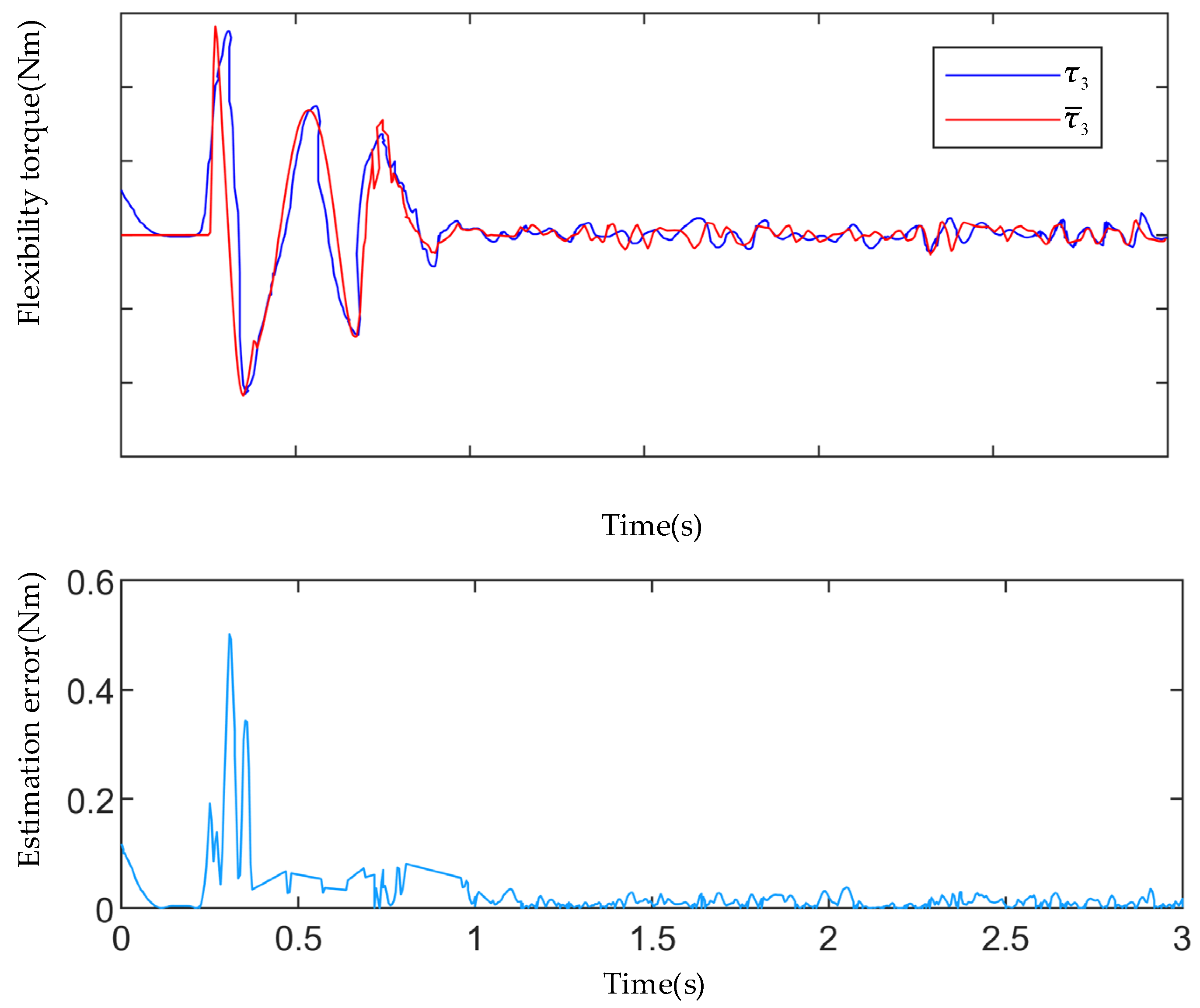
. Then, we can estimate the flexible force and the corresponding estimation error, as shown in Figure 6, Figure 7, Figure 8 and Figure 9.
Figure 6, Figure 7, Figure 8 and Figure 9 demonstrate the performance of the proposed observer-based approach; when the continuous contact force acts on the FDCDM, four dampers and springs will output flexible force and torque. From the results, we can see that the proposed estimation algorithm will produce a large error at the beginning; this is because the algorithm needs a short time to collect enough dynamic information. After a short delay, the estimation error converges to a small range. Table 2 shows the mean square error (MSE) of each joint. Due to the initial errors showing randomness, we just used the error close to the steady state (after 0.5 s) to calculate the MSE. This verified the effectiveness and low latency of the proposed unknown input observer in terms of flexible force estimation.
Remark 1:
The formula for the MSE in this paper is MSE = 1 N n = 1 N ( χ ( n ) χ ¯ ( n ) ) 2 , where χ ( n ) is the actual flexible force and χ ¯ ( n ) is the estimated flexible force.
Remark 2:
From Table 2 we can see that the MSE of damper 1 is large compared with the other dampers, which is because the estimated errors of damper 1 between 0.5 and 1 s are noticeably larger than the other dampers. The reason for this may be that damper 1 represents the x axis of the cross-axis structure, and in the collision test, the contact force on the x-axis is larger, causing the angle of damper 1 to change significantly, and indirectly leading to a larger error in the estimated value between 0.5 and 1 s.
The RLS algorithm runs with a null Π ^ i , j [ 0 ] and an initial covariance matrix P i , j [ k ] = 10 6 I 4 , and the sampling period is set as T = 10 2 ( s ) 
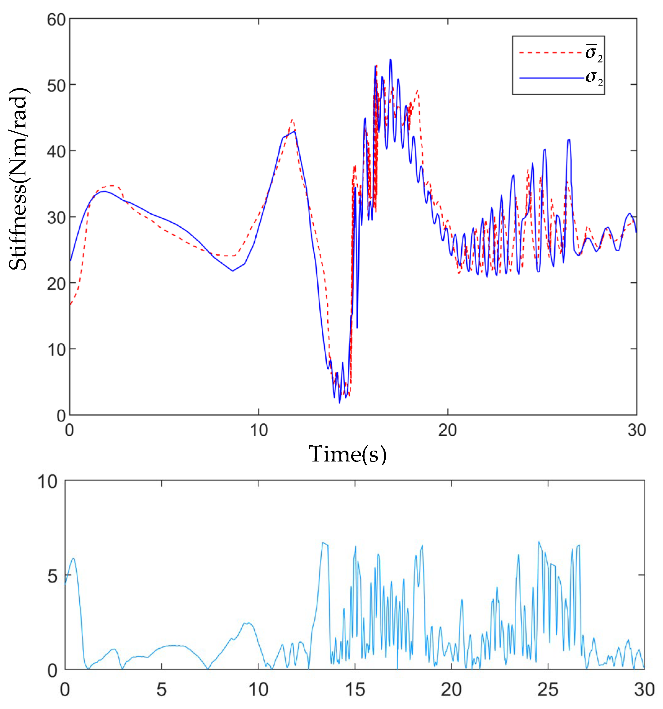
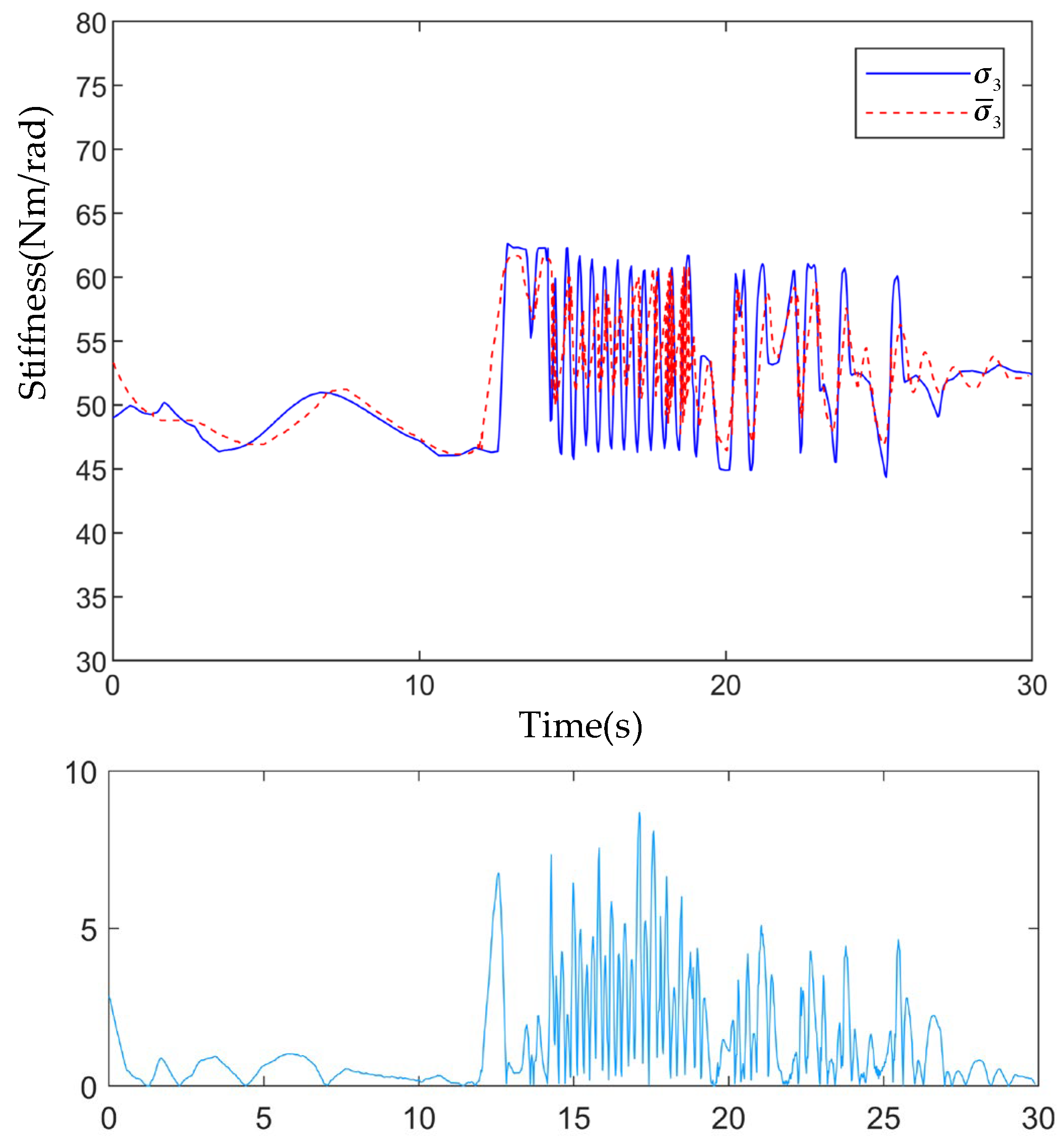
. The estimated results are shown in Figure 10, Figure 11, Figure 12 and Figure 13.
Figure 10, Figure 11, Figure 12 and Figure 13 illustrate that the proposed method could accurately track the stiffness due to the imprecise initialization of its parameters, and the algorithm itself shows good performance with the error controlled at about 5%. This verified the effectiveness and low latency of the proposed unknown input observer and recursive least square (RLS) algorithm.

5. Conclusions

In this article, a full-dimensional controllable damping mechanism (FDCDM) with a cross-axis structure is introduced into the end joint of the spacecraft-manipulator system (SMS), and the whole-body dynamic model of the spacecraft-manipulator system (SMS) with a full-dimensional damping mechanism (SMS-FDCDM) is established by using the Kane method. Then, the problem of estimating the stiffness in flexible robot joints driven by the full-dimensional controllable damping mechanism (FDCDM) was addressed by using the proposed unknown input observer and recursive least square (RLS) algorithm in this work. The proposed solution included a delayed unknown input observer (UIO), reconstructing flexibility torques at each damper, and an RLS algorithm, which subsequently obtained stiffness from a parameterization of the torque expression with respect to the flexible transmission. The simulation results show that both flexibility torque and stiffness are well estimated. Moreover, the solution has shown several advantages. First, the estimation process does not require speed and force sensors, since the unknown input observer (UIO) simultaneously estimates the speed and reconstructs the flexibility torque. Secondly, the variable parameter matrix of the observer is updated by a model-based neural learning algorithm, which significantly increases the estimation accuracy. Therefore, the numerical simulation of the collision experiment demonstrates the superior performance of the proposed approach. Then, the spacecraft-manipulator system used for grasping tasks can be required to keep the base and link positions stable, while accurately varying the joint stiffness and damping. Therefore, this work is significant for space noncooperative target capturing tasks.

Author Contributions

Conceptualization, R.C. and M.C.; methodology, R.C.; software, R.C.; validation, R.C., M.C., Q.J. and X.Z.; formal analysis, R.C.; investigation, M.C.; resources, R.C.; data curation, R.C.; writing—original draft preparation, R.C.; writing—review and editing, M.C.; visualization, Q.J. and X.Z.; supervision, Q.J. and X.Z.; project administration, M.C.; funding acquisition, M.C. and X.Z. All authors have read and agreed to the published version of the manuscript.

Funding

This work is partially supported by the Major Project of the New Generation of Artificial Intelligence, China (No. 2018AAA0102905), the National Natural Science Foundation of China (Grant No. 51875046), and the Natural Science Foundation of Beijing Municipality (Grant No. 3202021). The authors would like to thank the anonymous reviewers for their valuable comments to improve the quality of this paper.

Institutional Review Board Statement

Not applicable.

Informed Consent Statement

Not applicable.

Conflicts of Interest

The authors declare no conflict of interest.

References

  1. Jiang, H.; Hawkes, E.W.; Fuller, C. A robotic device using gecko-inspired adhesives can grasp and manipulate large objects in microgravity. Sci. Robot. 2017, 2, 4545. [Google Scholar] [CrossRef] [PubMed] [Green Version]
  2. Long, A.; Richards, M.; Hastings, D.E. On-orbit servicing: A new value proposition for satellite design and operation. J. Spacecr. Rockets 2007, 44, 964–976. [Google Scholar] [CrossRef] [Green Version]
  3. Flores-Abad, A.; Ma, O.; Pham, K.; Ulrich, S. A review of space robotics technologies for on-orbit servicing. Prog. Aerosp. Sci. 2014, 68, 1–26. [Google Scholar] [CrossRef] [Green Version]
  4. Ruggiero, F.; Lippiello, V.; Ollero, A. Aerial manipulation: A literature review. IEEE Robot. Autom. Lett. 2018, 3, 1957–1964. [Google Scholar] [CrossRef] [Green Version]
  5. Colonel, L.; Imburgia, J.S. Space debris and its threat to national security: A proposal for a binding international agreement to clean up the junk. Vanderbilt. J. Transnatl. Law 2011, 44, 6054–6064. [Google Scholar]
  6. Hobbs, S. Disposal orbits for geo spacecraft: A method for evaluating the orbit height distributions resulting from implementing iadc guidelines. Adv. Space Res. 2010, 45, 1042–1049. [Google Scholar] [CrossRef] [Green Version]
  7. Benvenuto, R.; Salvi, S. Dynamics analysis and gnc design of flexible systems for space debris active removal. Acta Astronaut. 2015, 110, 247–265. [Google Scholar] [CrossRef]
  8. Shan, M.; Jian, G.; Gill, E. Deployment dynamics of tethered-net for space debris removal. Acta Astronaut. 2017, 132, 293–302. [Google Scholar] [CrossRef]
  9. Chen, Q.; Zhang, Q.; Gao, Q.; Feng, Z.; Tang, Q. Design and optimization of a space net capture system based on a multi-objective evolutionary algorithm. Acta Astronaut. 2020, 167, 286–295. [Google Scholar] [CrossRef]
  10. Shan, M.; Shi, L. Comparison of Tethered Post-Capture System Models for Space Debris Removal. Aerospace 2022, 9, 33. [Google Scholar] [CrossRef]
  11. Ru, M.; Zhan, Y.; Cheng, B.; Zhang, Y. Capture Dynamics and Control of a Flexible Net for Space Debris Removal. Aerospace 2022, 9, 299. [Google Scholar] [CrossRef]
  12. Zhang, X.; Liu, J.; Feng, J. Effective capture of nongraspable objects for space robots using geometric cage pairs. IEEE/ASME Trans. Mechatron. 2019, 25, 95–107. [Google Scholar] [CrossRef] [Green Version]
  13. Choi, J.; Jung, J.; Lee, D. Articulated linkage arms based reliable capture device for janitor satellites. Acta Astronaut. 2019, 163, 91–99. [Google Scholar] [CrossRef]
  14. Grebenstein, M. The DLR hand arm system. In Proceedings of the 2011 IEEE International Conference on Robotics and Automation, Shanghai, China, 9–13 May 2011; pp. 3175–3182. [Google Scholar]
  15. Petit, F.; Daasch, A.; Albu-Schäffer, A. Backstepping control of variable stiffness robots. IEEE Trans. Control Syst. Technol. 2015, 23, 2195–2202. [Google Scholar] [CrossRef]
  16. Kim, J.; Croft, A.E. Full-state tracking control for flexible joint robots with singular perturbation techniques. IEEE Trans. Control Syst. Technol. 2019, 27, 63–73. [Google Scholar] [CrossRef]
  17. Ming, C.; Wu, X.Y. Modeling and self-learning soft-grasp control for free-floating space manipulator during target capturing using variable stiffness method. IEEE Access 2018, 6, 7044–7054. [Google Scholar]
  18. Balamurugan, L.; Jancirani, J.; Eltantawie, M.A. Generalized magnetorheological (MR) damper model and its application in semi-active control of vehicle suspension system. Int. J. Automot. Technol. 2014, 15, 419–427. [Google Scholar] [CrossRef]
  19. Huynh, T.C.N.; Sharf, I. Capture of Spinning Target with Space Manipulator using Magneto Rheological Damper. In Proceedings of the AIAA Guidance, Navigation, and Control Conference, Toronto, ON, Canada, 2–5 August 2010. [Google Scholar]
  20. Maciejewski, I.; Pecolt, S.; Krzyżyński, T. Controlling the vibration of a seat suspension system with the use of a magneto-rheological damper. Arch. Automot. Eng. Arch. Motoryz. 2017, 77, 85–95. [Google Scholar]
  21. Dwivedy, S.K.; Eberhard, P. Dynamic analysis of flexible manipulators, a literature review. Mech. Mach. Theory 2006, 41, 749–777. [Google Scholar] [CrossRef]
  22. Korayem, M.H.; Shafei, A.M.; Dehkordi, S.F. Systematic modeling of a chain of N-flexible link manipulators connected by revolute–prismatic joints using recursive gibbsappell formulation. Arch. Appl. Mech. 2014, 84, 187–206. [Google Scholar] [CrossRef]
  23. Zhang, D.G. Recursive Lagrangian dynamic modeling and simulation of multi-link spatial flexible manipulator arms. Appl. Math. Mech. 2009, 30, 1283–1294. [Google Scholar] [CrossRef]
  24. Yan, Z.; Lai, X.; Meng, Q. Tracking control of single-link flexible-joint manipulator with unmodeled dynamics and dead zone. Int. J. Robust Nonlinear Control 2020, 31, 1270–1287. [Google Scholar] [CrossRef]
  25. Bian, Y.; Gao, Z.; Lv, X. Theoretical and experimental study on vibration control of flexible manipulator based on internal resonance. J. Vib. Control 2018, 24, 3321–3337. [Google Scholar] [CrossRef]
  26. Chu, A.M.; Bien, D.X. New development of the dynamic modeling and the inverse dynamic analysis for flexible robot. Int. J. Adv. Robot. Syst. 2020, 17. [Google Scholar] [CrossRef]
  27. Deng, W.; Yao, J. Extended-state-observer-based adaptive control of electrohydraulic servomechanisms without velocity measurement. IEEE-ASME Trans. Mechatron. 2019, 25, 1151–1161. [Google Scholar] [CrossRef]
  28. Deng, W.; Yao, J.; Ma, D. Time-varying input delay compensation for nonlinear systems with additive disturbance: An output feedback approach. Int. J. Robust Nonlinear Control 2018, 28, 31–52. [Google Scholar] [CrossRef]
  29. Liu, Y.; Li, Z.; Su, H. Whole body control of an autonomous mobile manipulator using series elastic actuators. IEEE-ASME Trans. Mechatron. 2021, 26, 657–667. [Google Scholar] [CrossRef]
  30. Grioli, G.; Bicchi, A. A real-time parametric stiffness observer for VSA devices. In Proceedings of the 2011 IEEE International Conference on Robotics and Automation, Shanghai, China, 9–13 May 2011; pp. 5535–5540. [Google Scholar]
  31. Grosu, V.; Rodriguez-Guerrero, C.; Grosu, S.; Vanderborght, B. Design of smart modular variable stiffness actuators for robotic-assistive devices. IEEE/ASME Trans. Mechatron. 2017, 22, 1777–1785. [Google Scholar] [CrossRef]
  32. Ménard, T.; Grioli, G.; Bicchi, A. A stiffness estimator for agonistic–antagonistic variable-stiffness-actuator devices. IEEE Trans. Robot. 2014, 30, 1269–1278. [Google Scholar] [CrossRef] [Green Version]
  33. Fagiolini, A.; Trumić, M.; Jovanović, K. An input observer-based stiffness estimation approach for flexible robot joints. IEEE Robot. Autom. Lett. 2020, 5, 1843–1850. [Google Scholar] [CrossRef]
  34. Liu, Z.; Jin, H.; Liu, Y. An Online Stiffness Estimation Approach for Variable Stiffness Actuators Using Lever Mechanism. IEEE Robot. Autom. Lett. 2022, 7, 6709–6717. [Google Scholar] [CrossRef]
Figure 1. The 3D model of the full-dimensional controllable damping mechanism (FDCDM).
Aerospace 09 00726 g001
Figure 2. The exploded drawing of the controllable damping mechanism with cross-axis structure; (a) rotary x-axis and rotary y-axis joint of cross-axis structure; (b) rotary z axis of cross-axis structure; (c) sliding z structure; 1. rotating MR damper; 2. electromagnetic clutch; 3. torsion spring; 4. torsion spring fixings; 5. encoder; 6. bracket; 7. coupling; 8. deep-groove ball bearing; 9. sleeve; 10. damping z axis; 11. electromagnetic brake slider; 12. linear MR damper; 13. linear spring; 14. linear displacement sensor; 15. slide rail.
Aerospace 09 00726 g002
Figure 3. The conversion diagram of the six-dimensional damping force.
Aerospace 09 00726 g003
Figure 4. The 3D model of spacecraft-manipulator system with FDCDM (SMS-FDCDM).
Aerospace 09 00726 g004
Figure 5. The equivalent diagram of the spacecraft-manipulator system with FDCDM (SMS-FDCDM).
Aerospace 09 00726 g005
Figure 6. The actual flexible torque τ 1 and the estimated flexible torque τ ¯ 1 of the first damper and the corresponding estimation error using the proposed observer-based estimation algorithm.
Aerospace 09 00726 g006
Figure 7. The actual flexible torque τ 2 and the estimated flexible torque τ ¯ 2 of the second damper and the corresponding estimation error using the proposed observer-based estimation algorithm.
Aerospace 09 00726 g007
Figure 8. The actual flexible torque τ 3 and the estimated flexible torque τ ¯ 3 of the third damper and the corresponding estimation error using the proposed observer-based estimation algorithm.
Aerospace 09 00726 g008
Figure 9. The actual flexible force F 4 and the estimated flexible force F ¯ 4 of the end damper and the corresponding estimation error using the proposed observer-based estimation algorithm.
Aerospace 09 00726 g009
Figure 10. The actual stiffness σ 1 and the estimated stiffness σ ¯ 1 of the first joint of FDCDM and the corresponding estimation error using the proposed observer-based estimation algorithm.
Aerospace 09 00726 g010
Figure 11. The actual stiffness σ 2 and the estimated stiffness σ ¯ 2 of the second joint of FDCDM and the corresponding estimation error using the proposed observer-based estimation algorithm.
Aerospace 09 00726 g011
Figure 12. The actual stiffness σ 3 and the estimated stiffness σ ¯ 3 of the third joint of FDCDM and the corresponding estimation error using the proposed observer-based estimation algorithm.
Aerospace 09 00726 g012
Figure 13. The actual stiffness σ 4 and the estimated stiffness σ ¯ 4 of the end joint of FDCDM and the corresponding estimation error using the proposed observer-based estimation algorithm.
Aerospace 09 00726 g013
Table 1. Dynamic parameters of the SMS-FDCDM model.
Rigid Bodies k m k / kg I k / kg m 2 d k / m r k / m
xyz
1-base10042504261.8
2-joint 11011100
3-joint 21011100
4-damper 11.60.030.050.0400
5-damper 21.60.030.050.0600
6-damper 31.60.020.060.060.420.32
7-damper 440.50.50.40.40.2
Table 2. MSE for estimation error of each joint.
Damper 1
( Nm 2 )
Damper 2
( Nm 2 )
Damper 3
( Nm 2 )
Damper 4
( N 2 )
MSE0.0540.0230.0260.042
Publisher’s Note: MDPI stays neutral with regard to jurisdictional claims in published maps and institutional affiliations.

