Numerical Comparison of Contact Force Models in the Discrete Element Method

Abstract

The discrete element method (DEM) is usually applied in analyzing the scientifical origin/evolution of the asteroids and the landing/sampling of the regolith. In order to manage the contact between the non-spherical granules, the Polygonal Contact Model (PCM) has been introduced into the DEM method. This paper applies four different contact force models in the newly-proposed DEM algorithm to analyze their difference and implication. The four contact force models include one linear model and three nonlinear models derived from the complete Mindlin–Deresiewicz equations. By considering the macroscopical results and calculation efficiency, the single-collision and multiple-collision cases are analyzed by comparing the four contact models. Specifically, the restitution coefficient, the angular velocity, the rebound angle, and the kinetic energy are applied as indicators for the single collision. The multiple-collision case is studied under the Brazil nut effect with ellipsoidal granules. Additionally, the softening feasibility is also discussed by decreasing the Young’s modulus of the material, mainly analyzing the outgoing results and the calculation efficiency.

1. Introduction

With the development of computing technologies, the discrete element method (DEM) has become one of the most popular approaches to studying the granular system [1]. In asteroid explorations, the DEM method is widely exploited in simulating the origin and evolution of the asteroids [2] and the interaction of the probe with the asteroid regoliths [3]. In this research, the soft-sphere model [4] describing the overlap and force change during the contact is usually applied, which is suitable for analyzing the regoliths composed of fine-grained particles. However, the regolith areas usually make up less than half of the asteroid surfaces, and the rubble-pile asteroids have pebbles/rocks/boulders with diverse sizes, geologic composition, and morphology [5,6,7]. In terms of these various structures, the soft-sphere model has disadvantages in reflecting their irregular characteristics. In order to efficiently manage the non-spherical granules, the Polygonal Contact Model (PCM) has been embedded into the DEM algorithm, which is applicable for the arbitrarily-shaped granules by applying the polyhedral models with triangular meshes [8].

In terms of the spherical/non-spherical DEM model, the essential mechanism is solving the contact force between these granules and applying Newton’s second law to update the states [9]. For calculating the contact force between two objects, Cundall and Strack proposed the linear spring–dashpot model in 1979, where the contact force depends on the normal/tangential displacement and the relative velocity [1]. Many works have tried to modify the model of Cundall and Strack by changing the equations of the spring/damping coefficients and the normal/tangential spring length, such as the works of Brendel and Dippel [10], Garc’ıa-Rojo et al. [11], and Brilliantov et al. [12]. These models usually introduce extra variables and are not very common in the practice of DEM. Based on the research of Cundall and Strack, Tsuji [13,14] introduced the nonlinear Hertzian contact model to calculate the normal force. The tangential spring stiffness is derived from the simplified non-slip Mindlin–Deresiewicz model [15]. The complete Mindlin–Deresiewicz model (referred to as the MD model, hereafter) was presented in 1952, which calculates the tangential force based on the loading/unloading/reloading histories with different expressions of the incremental stiffness [16]. In addition to applying a non-slip case like Tsuji, some subsequent studies have tried to refine or simplify this complete MD model. Maw et al. [17,18] presented the more complicated MBF model based on the complete MD model in 1976, which discretizes the time and space domain when handling the oblique impact between a sphere and a plane. The MBF model is time-consuming for the large-scale DEM simulations. Walton and Braun presented a revised tangential model based on the complete MD model with the constant normal force in 1981 [19]. They also presented the normal hysteresis model for the plastic deformation, which divided the processes into loading and unloading parts with different spring stiffness. For brevity, more details about the summarization of force models are neglected, which can be found in Kruggel-Emden et al. [20] and Zhang et al. [21].

Among the plenty of contact force models, the linear spring–dashpot model and Tsuji’s nonlinear model are commonly applied in the DEM software, such as the pkdgrav [22], the DEMbody [23], and the MatDEM [24]. Although many wonderful works have applied these DEM software programs [25,26,27], they usually focused on analyzing and explaining the simulation results instead of comparing the effects of the contact force models. However, the contact force determines the accelerations of the granules, playing an essential role in the DEM model. This paper aims to analyze the feasibility of the newly-proposed DEM+PCM method and investigate the influence of the different contact force models on this new DEM algorithm. The critical innovation is verifying the collision results of the DEM+PCM model by comparing them with the classical experiment values. Different contact force models are compared by the various collision indicators and the CPU calculation efficiency. Additionally, an approach to accelerate the computation is tested, i.e., the softening operation of the material. After the simulations and comparisons, this paper intends to select the contact force model with higher calculation efficiency and the reasonable softening interval for the DEM+PCM model when the simulation results remain similar.

Assuming that the contact surfaces are continuous and the penetration is far smaller than the dimensions of the contact particles, four force models are analyzed, including the linear spring–dashpot model, the nonlinear Hertzian contact with the tangential non-slip MD model, the revised MD model by Di Renzo and Di Maio, and the complete MD model. These models are selected because of their acceptable computation efficiency [28]. Section 2 discusses the four contact force models’ principles, equations, and parameters in detail. Section 3.1 reproduces the classical single-collision experiment of Kharaz et al. [29] to study the performance of the new DEM algorithm. Four contact force models are compared by applying the single-collision case. The softening operations of the Young’s modulus with the original and decreased integral step size are discussed, respectively. Section 3.2 studies the differences between the non-slip MD model and the complete MD model in the multiple collisions by applying the Brazil nut effect. The conclusions are summarized in Section 4.

2. Materials and Methods

The Polygonal Contact Model is a contact calculation model for complexly-shaped bodies applying the polyhedral model with triangular facets [8]. Zhang et al. [30] first introduced the PCM method in the simulations of the surface locomotion of the small body probe Dynamics of the lander MASCOT have been studied by applying the PCM model. Based on the PCM model, a series of studies have been implemented on the landing dynamics of asteroid landers [31,32,33]. These papers reflect the feasibility and efficiency of the PCM model. A detailed introduction to the PCM method is in [34]. The specific integration of the PCM algorithm into the DEM frame has been summarized by Zeng et al. [35,36], which is not the focus of this paper. This study compares four classical models for calculating the contact force by applying the DEM+PCM algorithm. The principles and equations of these models are analyzed respectively, hereafter.

2.1. Linear Spring–Dashpot Model

The linear spring–dashpot model proposed by Cundall and Strack et al. is similar to the Kelvin–Voigt model in rheology [37]. When two bodies i and j collide, the contact force F_c acting on the body i is solved in Equation (1):

$$\{\begin{array}{l}{\mathit{v}}_{\mathit{r}\mathit{i}\mathit{j}}={\mathit{v}}_{\mathit{i}}-{\mathit{v}}_{\mathit{j}},{\mathit{v}}_{\mathit{n}\mathit{i}\mathit{j}}=\left({\mathit{v}}_{\mathit{r}\mathit{i}\mathit{j}}\cdot \widehat{\mathit{n}}\right)\widehat{\mathit{n}}\\ {\mathit{v}}_{\mathit{t}\mathit{i}\mathit{j}}={\mathit{v}}_{\mathit{r}\mathit{i}\mathit{j}}-{\mathit{v}}_{\mathit{n}\mathit{i}\mathit{j}}+{\mathit{l}}_i\left({\mathit{\omega }}_{\mathit{i}}\times \widehat{\mathit{n}}\right)+{\mathit{l}}_j\left({\mathit{\omega }}_{\mathit{j}}\times \widehat{\mathit{n}}\right)\\ {\mathit{f}}_{\mathit{n}}=-K_n{\delta }_{nij}\widehat{\mathit{n}}-{\eta }_n{\mathit{v}}_{\mathit{n}\mathit{i}\mathit{j}}\\ {\mathit{f}}_{\mathit{t}}=\{\begin{array}{l}-K_t{\mathit{\delta }}_{tij}-{\eta }_t{\mathit{v}}_{\mathit{t}\mathit{i}\mathit{j}},K_t{\delta }_{tij}<\mu f_n\\ -\mu f_n\frac{{\mathit{\delta }}_{\mathit{t}\mathit{i}\mathit{j}}}{\left|{\mathit{\delta }}_{\mathit{t}\mathit{i}\mathit{j}}\right|},K_t{\delta }_{tij}\ge \mu f_n\end{array}\\ {\mathit{F}}_{\mathit{c}}={\mathit{f}}_{\mathit{n}}+{\mathit{f}}_{\mathit{t}}\end{array},$$

(1)

where v_rij is the relative velocity of the centroid before contact, and v_tij and v_nij are the tangential and normal components of v_rij, respectively. The parameters ω and l represent the angular velocity and the arm of force, respectively. The contact force F_c is constituted by the normal force f_n and the tangential friction f_t. As for f_t, the spring-damping tangential force is calculated until the dynamic friction condition is satisfied, i.e., the gross slip/slide occurs. The normal and tangential relative displacements are represented by δ_nij and δ_tij, respectively. The normal vector $\widehat{\mathit{n}}$ points from the centroid of i to j. The parameters K_n/K_t are the spring stiffnesses, η_n/η_t are the damping coefficients, and μ is the friction coefficient. The parameters K_n/K_t are constant in the linear model, depending on the applied materials. The damping coefficients η_n/η_t are usually set as the critical damping coefficients based on K_n/K_t [1].

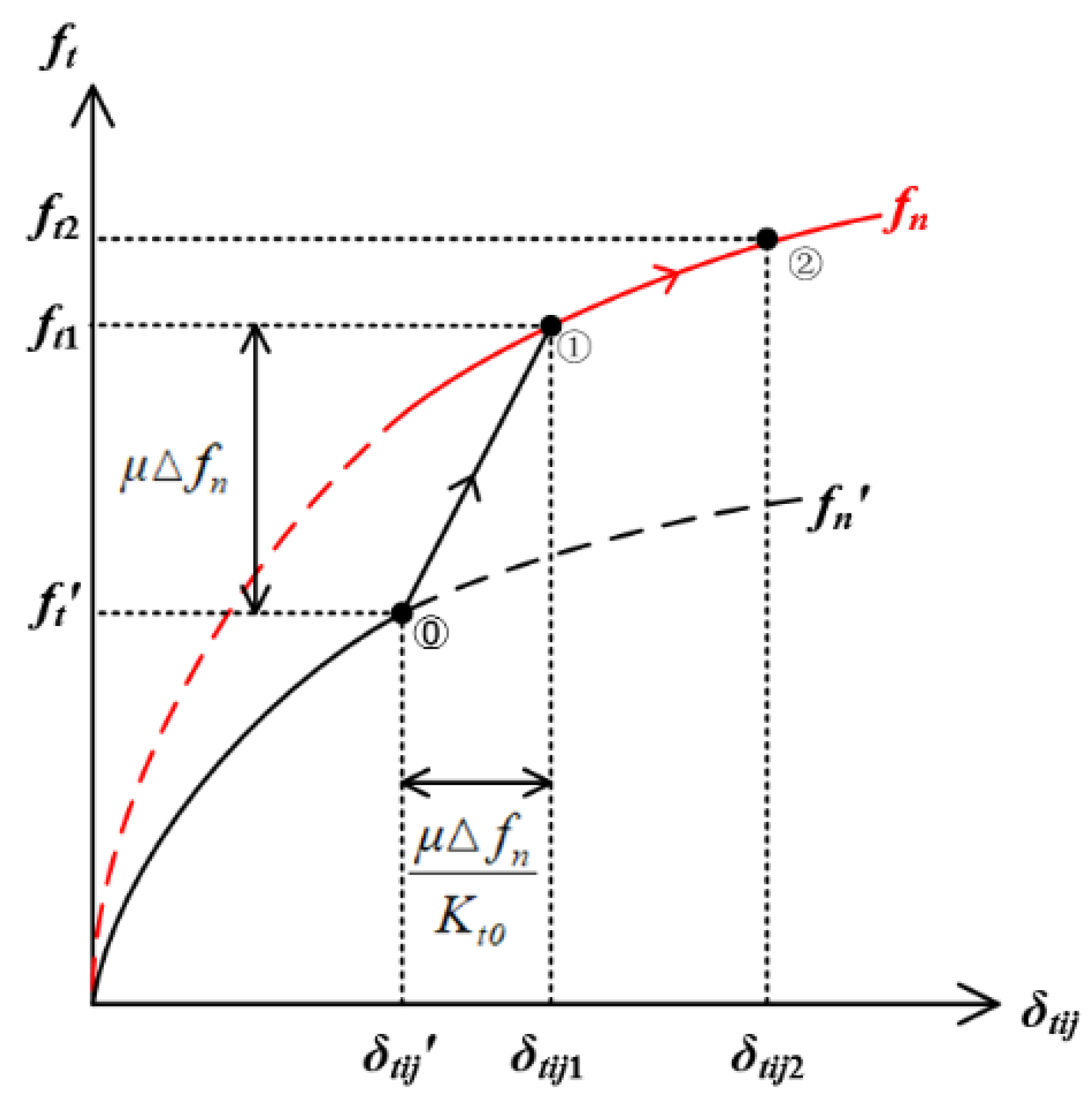
2.2. Mindlin–Deresiewicz Model (MD Model)

The complete tangential Mindlin–Deresiewicz model is complex, including the loading, unloading, and reloading phases when calculating the static friction. During the static friction phase, the contact area may be simultaneously constituted by the slip and non-slip regions, i.e., the micro-slip state exists. The MD model emphasizes that the system’s response to the current tangential change depends upon the previous loading history. The tangential force is calculated in an incremental approach, as shown in Equation (2). The damping part in Equation (1) is not considered in the original MD model:

$${\mathit{f}}_{\mathit{t},\mathit{M}\mathit{D}}={\mathit{f}}_{\mathit{t},\mathit{M}\mathit{D}}{}^{\prime }-K_{t,MD}△{\mathit{\delta }}_{\mathit{t}\mathit{i}\mathit{j}},$$

(2)

where ${\mathit{f}}_{\mathit{t},\mathit{M}\mathit{D}}{}^{\prime }$ and ${\mathit{f}}_{\mathit{t},\mathit{M}\mathit{D}}$ are the tangential force of body i in the last step and the current step, respectively. The symbol ${\mathit{f}}_{\mathit{t},\mathit{M}\mathit{D}}$ is applied to distinguish from the tangential force f_t with the damping part in Equation (1). The parameter $△{\mathit{\delta }}_{\mathit{t}\mathit{i}\mathit{j}}$ is the tangential displacement increment. The determination of the critical incremental stiffness K_t,MD depends on the contact scenario, classified by the change tendencies of the normal/tangential displacements. Taking the case when the normal and tangential displacements both increase as an example, the MD model is discussed in Equation (3):

$$\{\begin{array}{l}△{\mathit{\delta }}_{\mathit{t}\mathit{i}\mathit{j}}={\mathit{\delta }}_{\mathit{t}\mathit{i}\mathit{j}}-{\mathit{\delta }}_{\mathit{t}\mathit{i}\mathit{j}}{}^{\prime },△{\widehat{\mathit{\delta }}}_{\mathit{t}\mathit{i}\mathit{j}}=\frac{△{\mathit{\delta }}_{\mathit{t}\mathit{i}\mathit{j}}}{\left|△{\mathit{\delta }}_{\mathit{t}\mathit{i}\mathit{j}}\right|},△{\mathit{f}}_{\mathit{n}}={\mathit{f}}_{\mathit{n}}-{\mathit{f}}_{\mathit{n}}{}^{\prime } \\ G=\frac{E}{2(1+\upsilon )},\kappa =\frac{\left(1-{\upsilon }_i\right)/G_i+\left(1-{\upsilon }_j\right)/G_j}{\left(1-0.5{\upsilon }_i\right)/G_i+\left(1-0.5{\upsilon }_j\right)/G_j}\\ K_t{}_{,MD}=K_{t0}{\left(1-\frac{\kappa }{\mu }\frac{{\delta }_{tij}}{{\delta }_{nij}}\right)}^{1/2}=K_{t0}{\left(1-\frac{\left|f_{t,MD}{}^{\prime }-\mu △f_n△{\widehat{\delta }}_{tij}\right|}{\mu f_n}\right)}^{1/3}\\ {\mathit{f}}_{\mathit{t},\mathit{M}\mathit{D}}=\{\begin{array}{l}{\mathit{f}}_{\mathit{t},\mathit{M}\mathit{D}}{}^{\prime }-K_{t0}△{\mathit{\delta }}_{\mathit{t}\mathit{i}\mathit{j}},△{\delta }_{tij}<\frac{\mu △f_n}{K_{t0}}\\ {\mathit{f}}_{\mathit{t},\mathit{M}\mathit{D}}{}^{\prime }-\left[\mu △f_n+K_t{}_{,MD}\left(△{\delta }_{tij}-\frac{\mu △f_n}{K_{t0}}\right)\right]△{\widehat{\mathit{\delta }}}_{\mathit{t}\mathit{i}\mathit{j}},△{\delta }_{tij}\ge \frac{\mu △f_n}{K_{t0}}\end{array}\end{array},$$

(3)

Here, ${\mathit{\delta }}_{\mathit{t}\mathit{i}\mathit{j}}{}^{\prime }$ and ${\mathit{f}}_{\mathit{n}}{}^{\prime }$ donate the tangential displacement and the normal force of the last step. The parameters E, υ, and G represent the Young’s modulus, the Poisson’s ratio, and the shear modulus, respectively. The symbol ‘∆’ represents the increment of the corresponding parameter, and the superscript ‘^’ represents the normalized vector. The initial stiffness K_t0 defined in Equation (4) represents the non-slip contact case

$$\{\begin{array}{l}G=\frac{E}{2(1+\upsilon )},R_{eff}=\frac{R_i{R}_j}{R_i+R_j}\\ K_{t0}=8\frac{G_i{G}_j\sqrt{R_{eff}{\delta }_{nij}}}{G_j(2-{\upsilon }_i)+G_i(2-{\upsilon }_j)}\end{array},$$

(4)

Here, the parameter R_eff is the effective radius of the two interacted bodies.

Figure 1 intuitively illustrates the above process in Equation (3) when the normal and tangential displacements both increase. The black and red curves (color online) are the tangential loading curves f_t−δ_tij before and after the normal force increase (from ${\mathit{f}}_{\mathit{n}}{}^{\prime }$ to ${\mathit{f}}_{\mathit{n}}$). The tangential loading process with the same normal force is defined as the simple loading curve. The segments of curves marked with arrows represent the change of the static friction from the initial step (marked as ⓪) to the next step. The tangential displacement of the initial step is represented as ${\delta }_{tij}{}^{\prime }$. When the tangential displacement increment is less than $\frac{\mu △f_n}{K_{t0}}$ (between ${\mathit{\delta }}_{\mathit{t}\mathit{i}\mathit{j}}{}^{\prime }$ and ${\mathit{\delta }}_{\mathit{t}\mathit{i}\mathit{j}}{}_1$), the non-slip state is applied. The tangential force increases with the slope K_t0. If δ_tij is larger than δ_tij1, i.e., δ_tij2, the tangential force is constituted by two parts: f_t1 and the tangential force increment calculated by the residual tangential displacement (δ_tij2-δ_tij1) along the simple loading curve of ${\mathit{f}}_{\mathit{n}}$. In this case, the micro-slip appears, and the stiffness K_t,MD is applied during the simple loading phase. The detailed explanation of other displacement change scenarios is neglected for brevity, which can be found in [38]. The central principle is the incremental mechanism, distinguishing the non-slip and micro-slip states according to the tangential displacement in each step.

2.3. Hertzian Contact with the Non-Slip MD Model

In this model, the nonlinear Hertzian contact model is applied to calculate the normal contact force. The simplified non-slip MD model [13] with the damping influence is utilized for calculating the tangential force. This Hertzian and non-slip MD model is listed in Equation (5), which is similar to the Hunt and Crossley model [39] in the rheology with the nonlinear spring and damping elements:

$$\{\begin{array}{l}{\mathit{f}}_{\mathit{n}}=-K_n{\delta }_{nij}{}^{3/2}\widehat{\mathit{n}}-{\eta }_n{\mathit{v}}_{nij}\\ {\mathit{f}}_{\mathit{t}}=\{\begin{array}{l}-K_{t0}{\mathit{\delta }}_{\mathit{t}\mathit{i}\mathit{j}}-{\eta }_t{\mathit{v}}_{\mathit{t}\mathit{i}\mathit{j}},K_{t0}{\delta }_{tij}<\mu f_n\\ -\mu f_n\frac{{\mathit{\delta }}_{\mathit{t}\mathit{i}\mathit{j}}}{\left|{\mathit{\delta }}_{\mathit{t}\mathit{i}\mathit{j}}\right|},K_{t0}{\delta }_{tij}\ge \mu f_n\end{array}\end{array},$$

(5)

The applied parameters are defined as follows:

$$\{\begin{array}{l}{m}_{eff}=\frac{m_i{m}_j}{m_i+m_j}\\ K_n=\frac{4}{3}\frac{E_i{E}_j\sqrt{R_{eff}}}{E_i(1-{\upsilon }_i{}^2)+E_j(1-{\upsilon }_j{}^2)}\\ {\eta }_n=-\frac{\mathrm{l}\mathrm{n}{e}_n}{\sqrt{\mathrm{l}{\mathrm{n}}^2{e}_n+{\pi }^2}}\sqrt{5K_n{m}_{eff}}{\delta }_{nij}{}^{1/4}\\ {\eta }_t=-2\sqrt{\frac{5}{6}}\frac{\mathrm{l}\mathrm{n}{e}_t}{\sqrt{\mathrm{l}{\mathrm{n}}^2{e}_t+{\pi }^2}}\sqrt{K_{t0}{m}_{eff}}\end{array},$$

(6)

Here, when a granule contacts the plane, R_eff and m_eff equal the granule’s radius and mass, respectively. The restitution coefficients e_n and e_t are selected based on the experimental value of the applied material. The nonlinear damping coefficients η_n/η_t are related to the restitution coefficients [40,41]. The calculation of η_n/η_t is analyzed from Equation (7) to Equation (12). According to Tsuji et al., the nonlinear damping coefficient η_n is assumed to be $\alpha \left(e_n\right)\sqrt{m{K}_n}{\delta }_{nij}{}^{1/4}$ for the normal 1-D damped Hertzian oscillator with mass m. The dynamic equation is

$${\ddot{\delta }}_{nij}+\sqrt{\frac{K_n}{m}}\alpha (e_n){\delta }_{nij}{}^{1/4}{\dot{\delta }}_{nij}+\frac{K_n}{m}{\delta }_{nij}{}^{3/2}=0,$$

(7)

where α(e_n) is a parameter determined by e_n. Considering the relationship between the position and velocity, Equation (7) is rewritten as

$$\{\begin{array}{l}{v}_n=\frac{d{\delta }_{nij}}{dt}\\ v_n\frac{d{v}_n}{d{\delta }_{nij}}+\sqrt{\frac{K_n}{m}}\alpha (e_n){\delta }_{nij}{}^{1/4}{v}_n+\frac{K_n}{m}{\delta }_{nij}{}^{3/2}=0\end{array},$$

(8)

Supposing that ${\delta }_{nij}(t)={\left(\frac{5}{4}\right)}^{2/5}y{(t)}^{4/5}$, Equation (8) is converted into Equation (9) [42]:

$$v_n\frac{d{v}_n}{dy}+\frac{2}{\sqrt{5}}\sqrt{\frac{K_n}{m}}\alpha (e_n)v_n+\frac{K_n}{m}y=0,$$

(9)

Analogous with the linear spring–dashpot model (the damping coefficient in the linear model is introduced in Appendix A), the relationship between α and e_n is derived, and the nonlinear η_n is obtained in Equation (10)

$$\{\begin{array}{l}\alpha (e_n)=\frac{-\sqrt{5}\mathrm{l}\mathrm{n}{e}_n}{\sqrt{\mathrm{l}{\mathrm{n}}^2{e}_n+{\pi }^2}}\\ {\eta }_n=\alpha \left(e_n\right)\sqrt{m{K}_n}{\delta }_{nij}{}^{1/4}=-\frac{\mathrm{l}\mathrm{n}{e}_n}{\sqrt{\mathrm{l}{\mathrm{n}}^2{e}_n+{\pi }^2}}\sqrt{5K_{n}m}{\delta }_{nij}{}^{1/4}\end{array},$$

(10)

In terms of the tangential force, Tsuji et al. set η_t identical to η_n. In this study, η_t is solved from the equivalent stiffness K_e, which is defined below

$$\{\begin{array}{l}{F}_{Hertz}=K_n{\delta }_{nij}{}^{3/2}\\ K_e=\frac{d{F}_{Hertz}}{d{\delta }_{nij}}=2\frac{E_i{E}_j\sqrt{R_{ij}}}{E_i(1-{\upsilon }_i{}^2)+E_j(1-{\upsilon }_j{}^2)}{\delta }_{nij}{}^{1/2}\end{array},$$

(11)

Substituting K_e into Equation (10), η_n could be rewritten as

$${\eta }_n=-2\sqrt{\frac{5}{6}}\frac{\mathrm{l}\mathrm{n}{e}_n}{\sqrt{\mathrm{l}{\mathrm{n}}^2{e}_n+{\pi }^2}}\sqrt{K_{e}m},$$

(12)

When calculating η_t, the relationship between the damping coefficient η, the restitution coefficient e, and the equivalent stiffness K_e in Equation (12) remains the same. Based on Equation (5), K_e is supposed to be K_t0, and η_t is solved by applying e_t, as shown in Equation (6) [43].

2.4. Hertzian Contact with the Revised MD Model

Prior works have intended to revise the non-slip MD model. In this study, the model revised by Di Renzo and Di Maio is applied [44,45], which alters the stiffness K_t0. For distinction with K_t0, this new tangential stiffness is represented by K_tA in Equation (13)

$$K_{tA}=\frac{16}{3}\frac{G_i{G}_j\sqrt{R_{eff}{\delta }_{nij}}}{G_j(2-{\upsilon }_i)+G_i(2-{\upsilon }_j)}=\frac{2}{3}{K}_{t0},$$

(13)

To derive the modification of Equation (13), Di Renzo and Di Maio firstly focused on the simple loading case with the fixed normal force. The tangential elastic force f_t0 and f_t,MD calculated by the non-slip MD model and the complete MD model are compared in Equation (14)

$$\{\begin{array}{l}{f}_{t0}=K_{t0}{\delta }_{tij}\\ f_{t,MD}={\displaystyle {\int }_0^{{\delta }_{tij}}{K}_{t,MD}d\delta =}\mu f_n\left[1-{\left(1-\frac{\kappa }{\mu }\frac{{\delta }_{tij}}{{\delta }_{nij}}\right)}^{3/2}\right]\end{array},$$

(14)

where f_t,MD is derived by integrating K_t,MD and the tangential displacement. When f_t0 and f_t,MD both reach the Coulomb limit μf_n, the two tangential displacements satisfy the following condition:

$${\delta }_{t0}=\frac{2}{3}{\delta }_{t,MD},$$

(15)

Here, δ_t0 and δ_t,MD represent the tangential displacements of the non-slip and complete simple loading MD model, respectively. From Equation (15), Di Renzo and Di Maio deduced that the applied K_t0 in the non-slip MD model should be multiplied by $\frac{2}{3}$.

According to Figure 1, when the normal force changes, the hypothesis of the simple loading history does not apply if $△{\delta }_{tij}<\frac{\mu △f_n}{K_{t0}}$. In this case, the f_t–δ_tij curve experiences the constant slope K_t0. Di Renzo and Di Maio have also revised this process. Assuming that the normal and tangential velocities have no changes in these steps with K_t0, the new tangential force f_t,MD equals $\frac{2}{3}{f}_{t0}$ as calculated in Equation (16):

$$\begin{array}{ll}{f}_{t,MD}& ={\displaystyle {\int }_0^{\tau }{K}_{t0}{v}_{tij}dt}\\ & =\frac{8G_i{G}_j\sqrt{R_{ij}}}{G_j(2-{\upsilon }_i)+G_i(2-{\upsilon }_j)}{v}_{tij}{\displaystyle {\int }_0^{\tau }\sqrt{{\delta }_{nij}}dt}\\ & =\frac{8G_i{G}_j{v}_{tij}\sqrt{R_{ij}}}{G_j(2-{\upsilon }_i)+G_i(2-{\upsilon }_j)}\sqrt{v_{nij}}{\displaystyle {\int }_0^{\tau }\sqrt{t}dt},\\ & =\frac{2}{3}{K}_{t0}{\delta }_{tij}\\ & =\frac{2}{3}{f}_{t0}\end{array}$$

(16)

Combining Equation (15) and Equation (16), the tangential spring stiffness applied in the revised MD model is altered to be K_tA. The algebraic expression of K_tA is as simple as K_t0, where only the current displacement is needed. Although the revised MD model has tried to consider the incremental steps in the complete MD model by integration, the accuracy of this revision remains to be confirmed when the PCM model is applied. Because the ideal simple loading phase barely exists, it is not precise to modify f_t,MD only from the tangential displacement relationship in Equation (15). Additionally, the normal and tangential velocity in Equation (16) virtually cannot remain identical even at the beginning steps with K_t0.

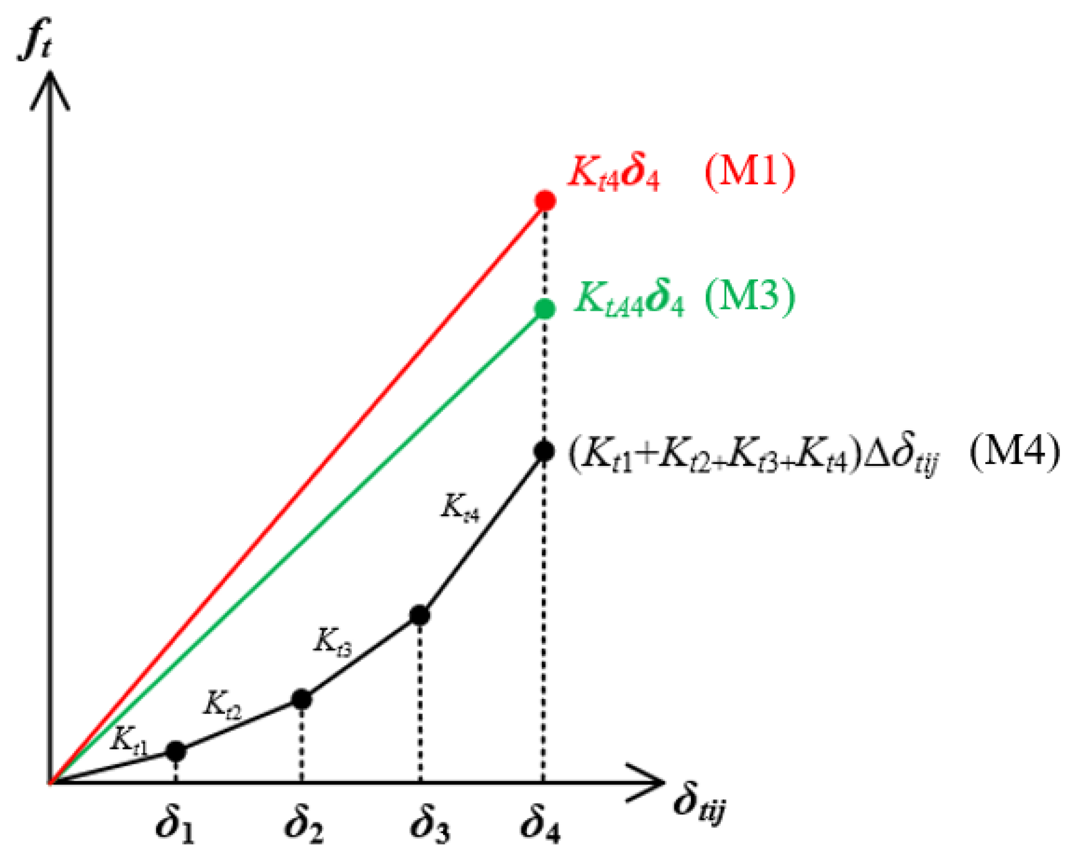
2.5. Difference of the Contact Force Models

The Hertzian contact with the non-slip MD model, the linear model, the Hertzian contact with the revised MD model, and the Hertzian contact with the complete MD model are named M1, M2, M3, and M4 in the following parts, respectively. The linear model M2 differs from the other three nonlinear models in terms of the normal force and the tangential spring/damping coefficients. The essential difference between the three nonlinear models M1/M3/M4 is mainly discussed below.

When calculating the elastic spring part of the tangential force, the non-slip model and the revised MD model depend on the current tangential displacement. In contrast, the complete MD model applies the tangential displacement increment. This is illustrated in Figure 2 by applying a loading case where the tangential and normal displacements both increase. Each time the normal force changes, the tangential displacement increment is assumed to be the same and not exceed $\frac{\mu △f_n}{K_{t0}}$. With the normal force increase, the tangential spring stiffness becomes larger. Therefore, in the complete MD model M4, four different tangential spring stiffnesses are applied based on the previous tangential force. However, in the model M1/M3, the total normal displacements after the fourth increase are applied to calculate the tangential spring stiffness, leading to the larger tangential force. Theoretically, the tangential force of M1/M3 will turn into dynamic friction earlier than M4.

Additionally, this study considers the damping influence in the four contact force models. The above expressions of M1 and M2 have already included the damping part. The applied tangential forces in M3 and M4 are rewritten in Equation (17) and Equation (18), respectively:

$${\mathit{f}}_{\mathit{t}}=\{\begin{array}{l}-K_{tA}{\mathit{\delta }}_{\mathit{t}\mathit{i}\mathit{j}}-{\eta }_t{\mathit{v}}_{\mathit{t}\mathit{i}\mathit{j}},K_{tA}{\delta }_{tij}<\mu f_n\\ -\mu f_n\frac{{\mathit{\delta }}_{\mathit{t}\mathit{i}\mathit{j}}}{\left|{\mathit{\delta }}_{\mathit{t}\mathit{i}\mathit{j}}\right|},K_{tA}{\delta }_{tij}\ge \mu f_n\end{array},$$

(17)

$${\mathit{f}}_{\mathit{t}}=\{\begin{array}{l}{\mathit{f}}_{\mathit{t},\mathit{M}\mathit{D}}-{\eta }_t{\mathit{v}}_{\mathit{t}\mathit{i}\mathit{j}},f_{t,MD}<\mu f_n\\ -\mu f_n\frac{{\mathit{\delta }}_{\mathit{t}\mathit{i}\mathit{j}}}{\left|{\mathit{\delta }}_{\mathit{t}\mathit{i}\mathit{j}}\right|},f_{t,MD}\ge \mu f_n\end{array},$$

(18)

3. Numerical Simulations

By applying the PCM+DEM method, the contact result will be influenced by the contact force, the integral step size, the body shape, the polyhedral model accuracy, etc. In the previous model comparison works, the single-collision case has been focused on widely, while the comparison of the multiple-collision is insufficient [20,46,47]. In order to verify the accuracy of the DEM+PCM algorithm and compare these contact force models, the classic experiment of Kharaz et al. [29,48] is reproduced to implement the single collision. Afterward, the multiple collisions are simulated by the Brazil nut effect, intending to find whether the contact force difference will accumulate in this case.

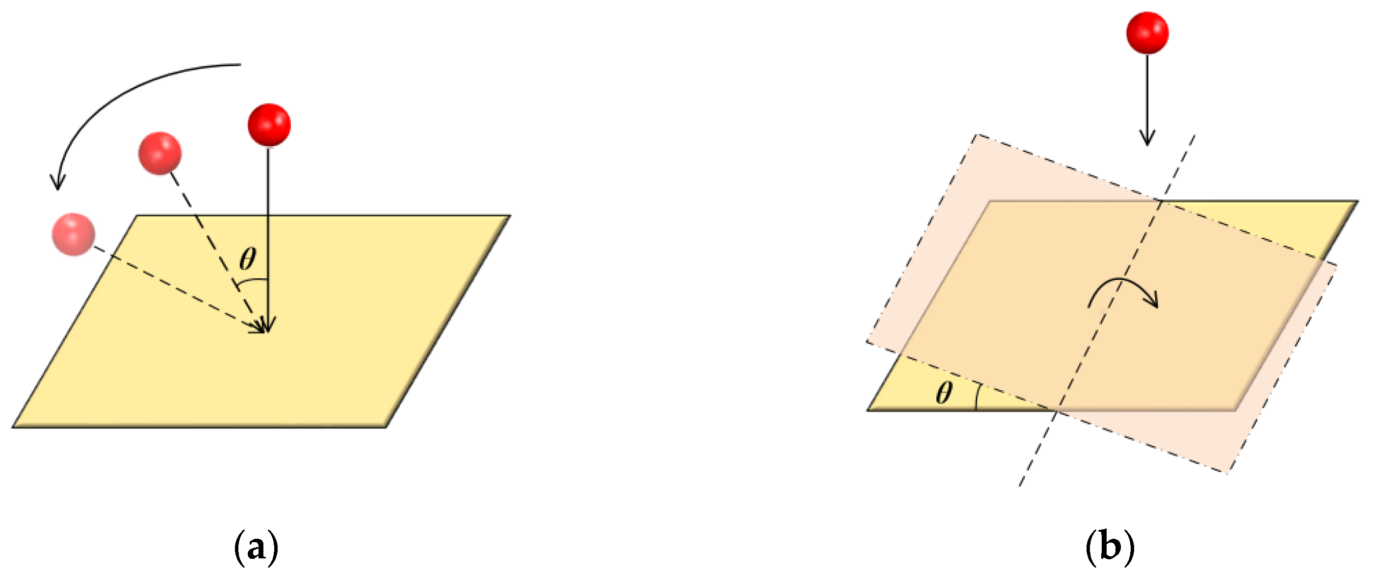
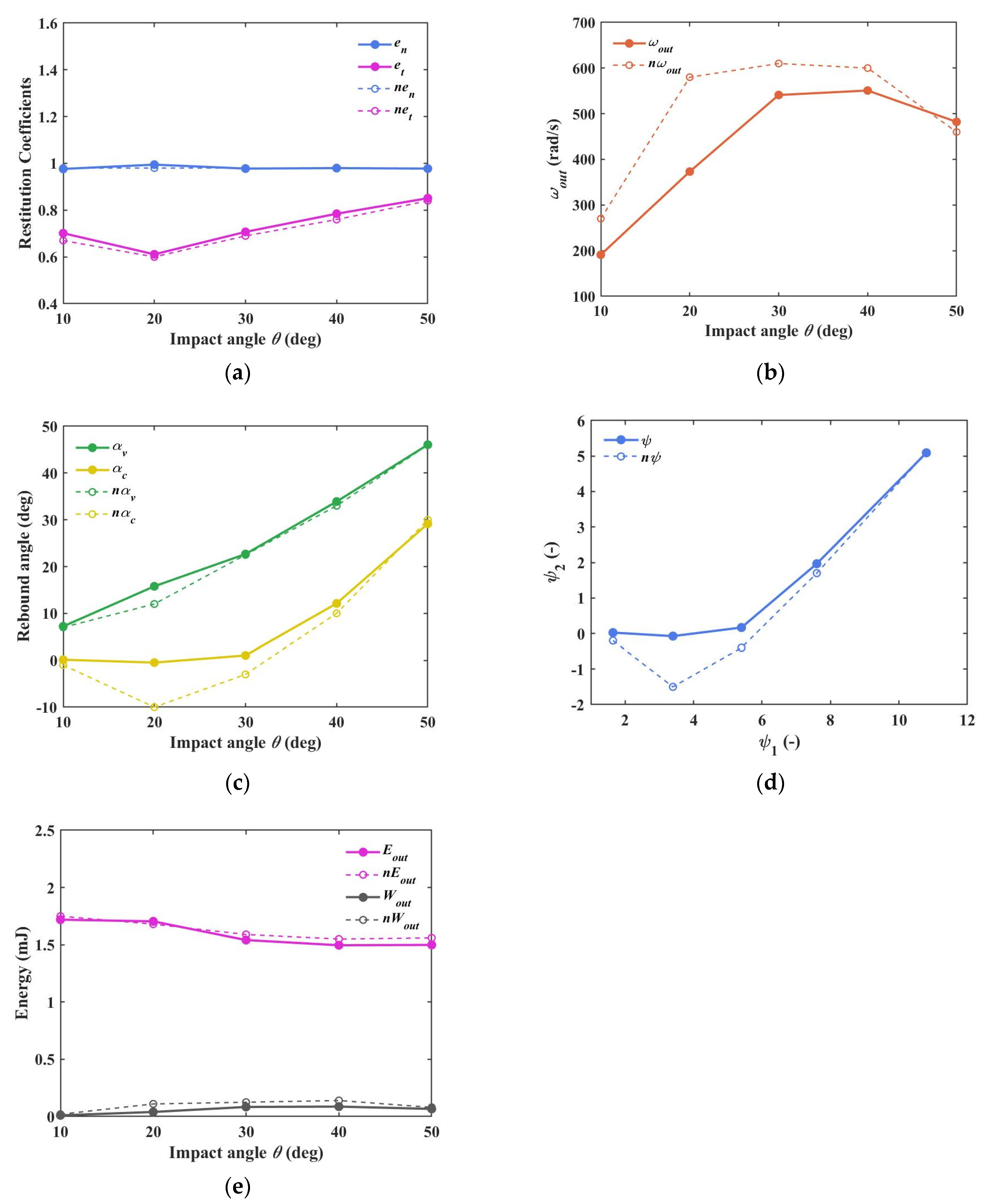
3.1. Single Collision Analyses

The representative experiment of Kharaz et al. describes an aluminum oxide sphere impacting a thick oblique soda-lime glass anvil. It has been widely used as the nominal experiment in many force comparison works [20]. In order to repeat the experiment, a regular sphere is analyzed, constituted by the polyhedral model. The contact detection is handled by the PCM model, with the calculation process consistent with that of the non-spherical body. The properties of the applied polyhedral models are listed in

Table 1. Characteristics of the material.

Material	Young’s Modulus (Gpa)	Poisson Ratio	Shear Modulus (Gpa)	Vertices	Facets
Aluminum oxide sphere	380	0.23	154	2562	5160
Soda-lime glass anvil	70	0.25	28	1906	3638

. The sphere’s diameter is 5 mm, and the density is 4000 kg∙m⁻³. The mass and the moment of inertia of the sphere are 2.29 × 10⁻⁴ kg and 5.73 × 10⁻¹⁰ kg∙m², respectively. The experiment intends to alter the oblique angle of the ingoing velocity of the sphere, like the operation in Figure 3a. However, it is not convenient for the equipment to change the velocity angle precisely. A substitute device was proposed in Figure 3b, applying a rotary table to alter the angle θ of the anvil plane. Initially, the sphere is held above the anvil by a small-diameter vacuum nozzle. The sphere is released vertically without spin and impacts the anvil at 4 m/s under 1 g.

In the experiment, the angle θ of the oblique plane increases from 10° to 50° with an interval of 10°. The dynamic equations of the sphere are given in Equation (19), according to Newton’s second law. The second-order leapfrog integrator [4] is applied to update the state of the sphere with the integral step size equal to 10⁻⁸ s:

$$\{\begin{array}{l}m\frac{{\mathrm{d}}^2\mathit{x}}{\mathrm{d}{t}^2}={\mathit{F}}_{\mathit{c}}+{\mathit{F}}_{\mathit{e}\mathit{x}\mathit{t}}\\ \mathit{I}\frac{\mathrm{d}\mathit{\omega }}{\mathrm{d}t}+\mathit{\omega }\times \left(\mathit{I}\mathit{\omega }\right)={\mathit{L}}_{\mathit{c}}+{\mathit{L}}_{\mathit{e}\mathit{x}\mathit{t}}\\ \frac{\mathrm{d}\mathit{q}}{\mathrm{d}t}=\frac{1}{2}\left[\begin{array}{llll}{q}_0\hfill & -q_1& -q_2& -q_3\\ q_1& q_0& -q_3& q_2\\ q_2& q_3& q_0& -q_1\\ q_3& -q_2& q_1& q_0\end{array}\right]\left[\begin{array}{l}0\\ \omega \end{array}\right]\end{array},$$

(19)

Here, m is the sphere’s mass, x and ω represent the position and angular velocity of the sphere, respectively, and q is the quaternion describing the attitude. The parameter I is the moment of inertia of the sphere. The external force (such as gravity) and corresponding torque are denoted by F_ext and L_ext, respectively. The contact force and torque are F_c and L_c, respectively.

The outgoing velocity, the angular velocity, the restitution coefficients, the rebound angle, the non-dimensional angle ψ proposed in the MBF model, and the energies are measured as the macroscopical indicators of the experiment.

(1)

Restitution coefficients;

The normal and tangential restitution coefficients e_n and e_t are defined in Equation (20) as

$$\{\begin{array}{l}\widehat{\mathit{t}}=\frac{{\mathit{V}}_{\mathit{i}\mathit{n}}-({\mathit{V}}_{\mathit{i}\mathit{n}}\cdot \widehat{\mathit{n}})\widehat{\mathit{n}}}{\left|{\mathit{V}}_{\mathit{i}\mathit{n}}-({\mathit{V}}_{\mathit{i}\mathit{n}}\cdot \widehat{\mathit{n}})\widehat{\mathit{n}}\right|}\\ e_n=\left|\frac{{\mathit{V}}_{\mathit{o}\mathit{u}\mathit{t}}\cdot \widehat{\mathit{n}}}{{\mathit{V}}_{\mathit{i}\mathit{n}}\cdot \widehat{\mathit{n}}}\right|\\ e_t=\left|\frac{{\mathit{V}}_{\mathit{o}\mathit{u}\mathit{t}}\cdot \widehat{\mathit{t}}}{{\mathit{V}}_{\mathit{i}\mathit{n}}\cdot \widehat{\mathit{t}}}\right|\end{array},$$

(20)

where V_in and V_out are the ingoing and outgoing velocities of the sphere’s centroid, respectively. The parameter $\widehat{\mathit{n}}$ is the normal vector of the oblique plane, $\widehat{\mathit{t}}$ represents the tangential direction of the ingoing velocity.

(2)

Rebound angle;

$$\{\begin{array}{l}\mathit{V}{\mathit{C}}_{\mathit{o}\mathit{u}\mathit{t}}={\mathit{V}}_{\mathit{o}\mathit{u}\mathit{t}}+{\mathit{\omega }}_{\mathit{o}\mathit{u}\mathit{t}}\times {\mathit{r}}_{\mathit{s}}\\ {\alpha }_v=\arctan \left(\frac{{\mathit{V}}_{\mathit{o}\mathit{u}\mathit{t}}\cdot \widehat{\mathit{t}}}{{\mathit{V}}_{\mathit{o}\mathit{u}\mathit{t}}\cdot \widehat{\mathit{n}}}\right)\\ {\alpha }_c=\arctan \left(\frac{\mathit{V}{\mathit{C}}_{\mathit{o}\mathit{u}\mathit{t}}\cdot \widehat{\mathit{t}}}{\mathit{V}{\mathit{C}}_{\mathit{o}\mathit{u}\mathit{t}}\cdot \widehat{\mathit{n}}}\right)\end{array},$$

(21)

Here, VC_out is the outgoing velocity of the contact patch considering the outgoing angular velocity ω_out, r_s is the vector pointing from the sphere centroid to the contact patch. The angles α_v and α_c are defined as the outgoing velocity angle and the outgoing angle, respectively.

(3)

Angle ψ in the MBF model;

$$\{\begin{array}{l}\kappa =\frac{(1-{\upsilon }_i)G_i+(1-{\upsilon }_j)G_j}{(1-0.5{\upsilon }_i)G_i+(1-0.5{\upsilon }_j)G_j}\\ {\psi }_1=\frac{\kappa }{\mu }\frac{{\mathit{V}}_{\mathit{i}\mathit{n}}\cdot \widehat{\mathit{t}}}{\left|{\mathit{V}}_{\mathit{i}\mathit{n}}\cdot \widehat{\mathit{n}}\right|}\\ {\psi }_2=\frac{\kappa }{\mu }\frac{\mathit{V}{\mathit{C}}_{\mathit{o}\mathit{u}\mathit{t}}\cdot \widehat{\mathit{t}}}{\left|{\mathit{V}}_{\mathit{i}\mathit{n}}\cdot \widehat{\mathit{n}}\right|}\end{array},$$

(22)

Here, ψ₁ and ψ₂ are the non-dimensional angles of incidence and reflection of the contact patch [22]. The subscript i and j refer to the sphere and the anvil plane, respectively.

(4)

Energies;

The outgoing translational kinetic energy E_out and the rotational kinetic energy W_out are defined in Equation (23)

$$\{\begin{array}{l}{E}_{out}=\frac{1}{2}m{\left|\mathit{V}{\mathit{C}}_{\mathit{o}\mathit{u}\mathit{t}}\right|}^2\\ W_{out}=\frac{1}{2}{\mathit{\omega }}_{\mathit{o}\mathit{u}\mathit{t}}{}^{\mathrm{T}}\mathit{I}{\mathit{\omega }}_{\mathit{o}\mathit{u}\mathit{t}}\end{array},$$

(23)

Here, m and I are the mass and the moment of inertia of the sphere, respectively.

3.1.1. Performance of the Hertzian Contact with the Non-Slip MD Model (M1)

The most commonly used Hertzian contact with the non-slip MD model (M1) is applied to verify the feasibility of the new DEM+PCM algorithm. Figure 4 illustrates the change tendencies of the indicators by applying M1. In the legend, the prefix n- (such as ne_n, ne_t, nω_out, etc) represents the results of the experiment.

In Figure 4, the results of reproducing the single-collision experiment validate the feasibility of this newly-presented DEM+PCM algorithm. The change tendencies of these indicators are similar to those of the experiment. Significantly, the restitution coefficients e_n in Figure 4a and the energies in Figure 4e have almost identical curves to those of the experiment values. The outgoing kinetic energies (the sum of E_out and W_out) are smaller than the ingoing kinetic energies (around 1.8 mJ), indicating that the energy decays when the potential energy almost remains identical. In terms of the outgoing angular velocity ω_out, when the impact angle θ is smaller than 50°, ω_out is smaller than the experiment results. When θ exceeds 30°, the deviations of ω_out are less than 70 rad/s. When θ is 10° and 20°, the deviations of ω_out are relatively larger, especially with 20° angle θ. The errors of ω_out lead to the differences in α_c, ψ₂, and W_out, i.e., the indicators calculated by the angular velocity. The influence of the facet number of the applied polyhedral model is not discussed temporarily. The specific values of these indicators in Figure 4 may fluctuate slightly when the facet number of the model in Table 1 is different. Discussions of the model’s facet number will be focused on in the future, which is not the main issue of this paper.

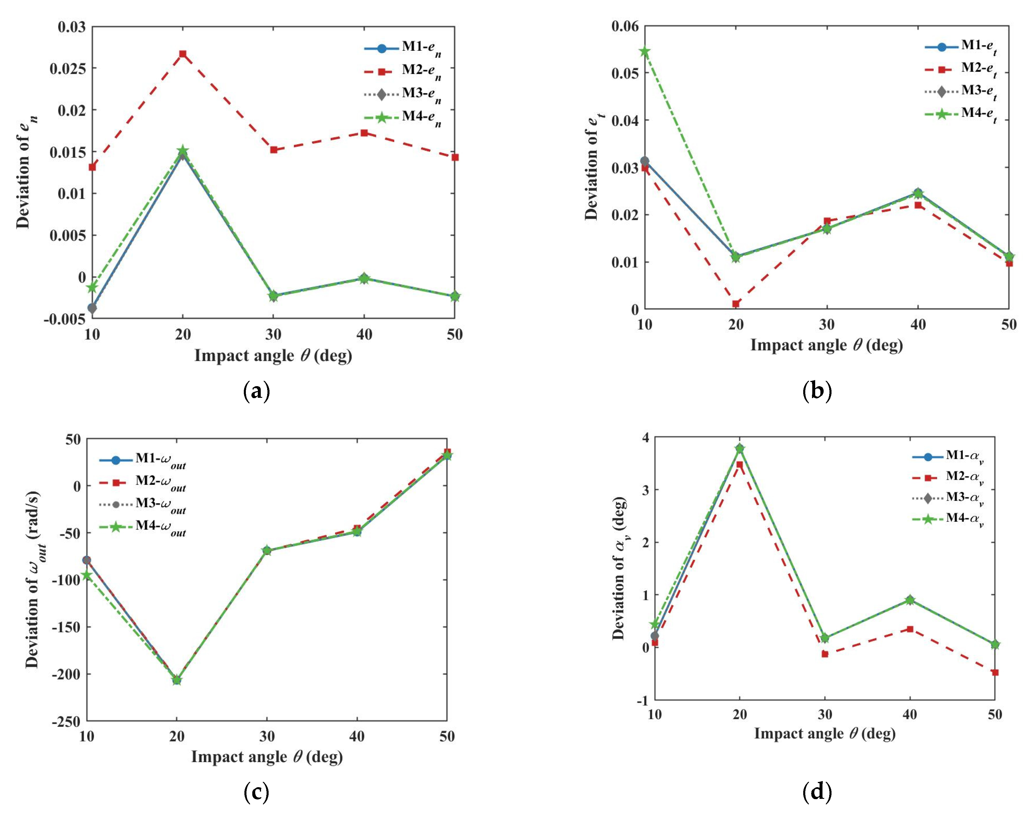
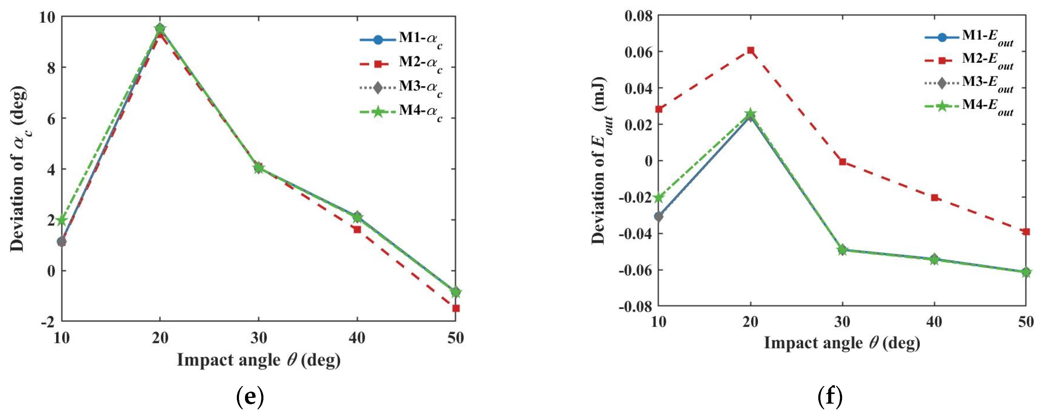
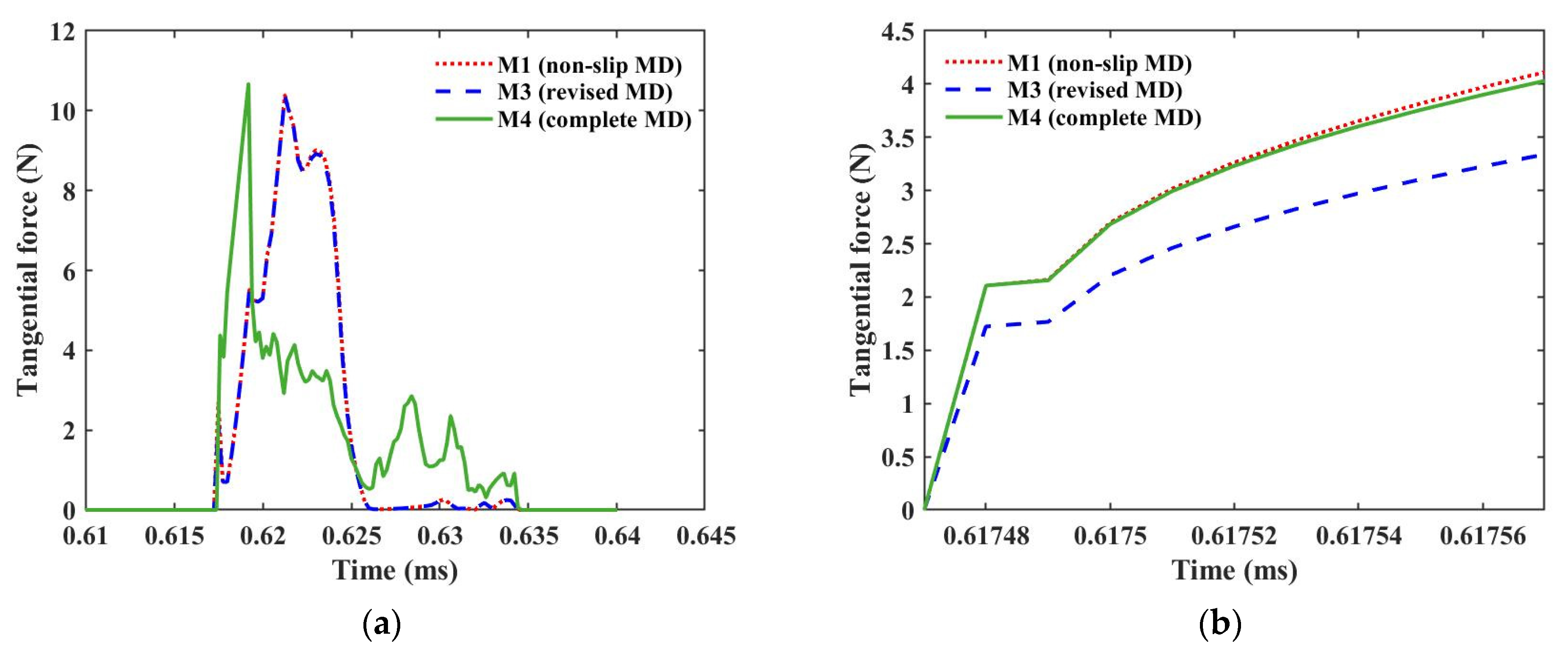
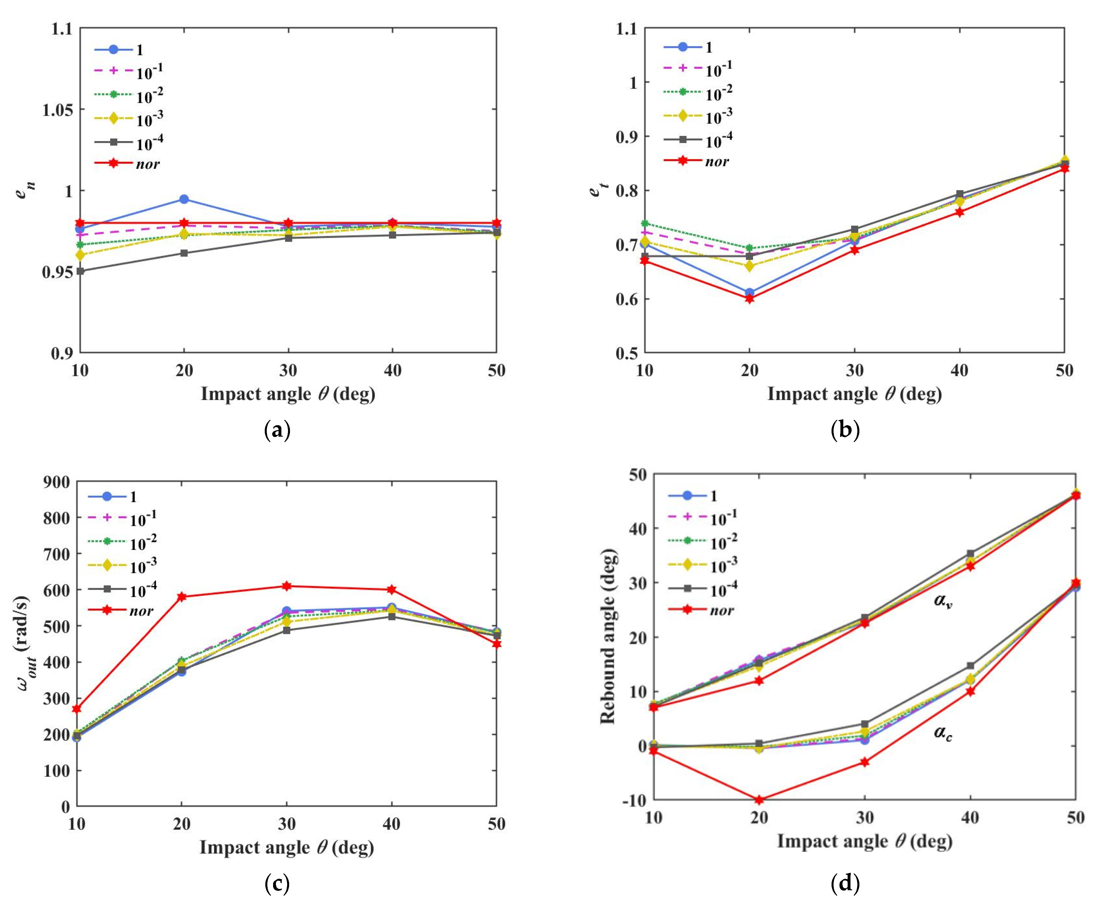
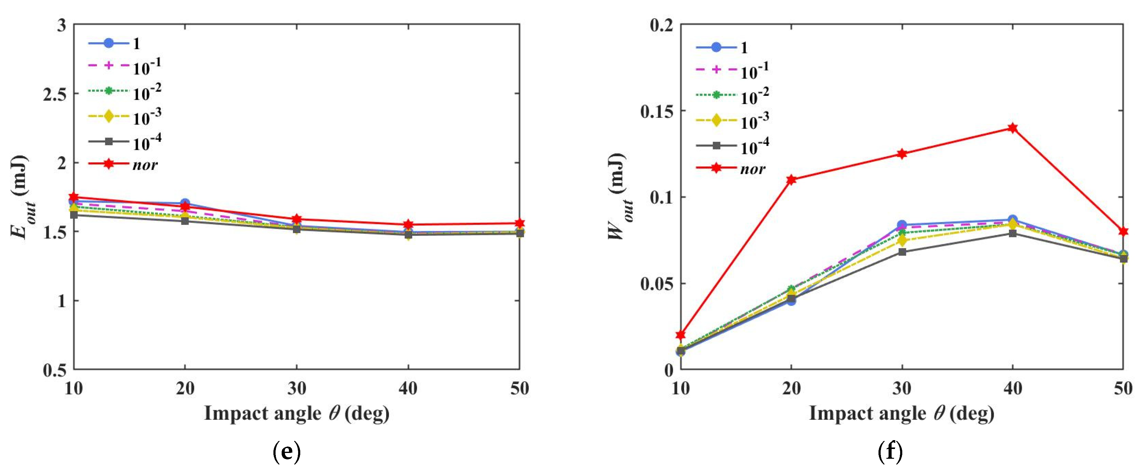
3.1.2. Comparison of the Four Contact Force Models

Deviations of the four contact force models in this single collision are analyzed and compared in Figure 5. The simulation value minus the experimental value derives the deviation. According to Di Renzo and Di Maio, the spring stiffness K_n and K_t in the linear model M2 are selected as 1.72 × 10⁷ N/m and 1.48 × 10⁷ N/m, respectively. They are obtained from the derivative of the force with respect to the corresponding displacement [45]. Based on K_n and K_t, the constant critical damping coefficients η_n/η_t in the linear model are solved as $2\sqrt{m{K}_n}$/$2\sqrt{m{K}_t}$, respectively.

The linear model M2 shows a significant difference from the nonlinear models: the deviations of e_n in Figure 5a and E_out with θ smaller than 30° in Figure 5f become larger. Among the three nonlinear models, the models M1 and M3 have nearly coincident result curves, indicating that the revision of the tangential spring stiffness in M3 has little influence. When θ is 10°, compared with the model M1/M3, the incremental model M4 reduces the deviations of e_n and E_out, while the errors of e_t and ω_out increase. If θ exceeds 20°, the results of the three nonlinear models are nearly the same. This phenomenon reflects that, in a single collision, the influence of the contact force model on the macroscopical indicators is evident when the oblique angle is less than 20°. The macroscopical difference in the contact force model can be neglected with the increase of the oblique angle. Afterward, the tangential forces of the three nonlinear models when the impact angle θ is 10° are illustrated and compared in Figure 6.

The collision phase lasts about 0.02 ms, from 0.617 ms to 0.635 ms. In Figure 6a, the tangential force curve of M4 shows a different change tendency compared with the models M1 and M3. The tangential force curve of M4 reaches the maximum value faster and experiences more waves when returning from the maximum value to zero. Figure 6b illustrates the static friction before the dynamic friction condition is satisfied. Influenced by different K_t, the force curve of M3 is below that of M1 proportionally. The slight difference between M4 and M1 increases gradually with time, similar to the analysis in Figure 2. Although the tangential forces of M1, M3, and M4 change differently, their values are all less than 11 N. The contact force difference during the short contact time does not lead to the variation of the macroscopical results after the collision.

The above discussions show that the three nonlinear contact force models result in different forces in this single collision. However, the short contact lasting time is not enough for the accumulation of the force difference to change the macroscopical indicators. For analyzing whether the contact force model will influence the CPU calculation efficiency, the CPU calculation times of the non-slip MD model (M1) and the complete MD model (M4) are illustrated and compared in Figure 7, respectively. The revised MD model M3 is not further discussed because its macroscopical indicators and force curves are all similar to M1.

In Figure 7, ten simulations under the same conditions are repeatedly implemented in each box. An Intel(R) Xeon(R) Silver 4216 CPU @ 2.10 GHz is utilized to implement the simulations. The CPU calculation times under M1 and M4 increase gradually with the impact angle, from 570 s to 610 s and from 590 s to 625 s, respectively. When the impact angle increases from 10° to 50°, the average CPU calculation times of M4 are 17 s, 3 s, 2 s, 12 s, and 12 s longer than M1. When comparing two calculation times, the increased calculation efficiency is defined as the time difference divided by the larger time. In Figure 7, by applying the average value of the box, the CPU calculation efficiency of the non-slip model M1 is increased by 3%, 0.5%, 0.3%, 2%, and 2%, respectively.

Based on the above discussions about the outgoing results and the calculation efficiency, the newly-presented DEM algorithm can capture the experiment’s characteristics in the single-collision case. By applying this DEM algorithm, the linear model shows the difference from the nonlinear models, mainly in the restitution coefficient e_n and the energy E_out. In this case, the stiffnesses K_n and K_t of the linear model are carefully determined by the nonlinear relationships between the force and the displacement [45]. However, the specific nonlinear relationships are usually unknown when directly applying the linear model instead of comparative analysis. The precise selection of K_n and K_t is difficult in the linear model, usually approximated as the Young’s modulus for the spherical particles with identical material. This simplification produces a difference compared to the actual contact dynamics, although some experimental stiffness ratio has been proposed for modification [49]. Therefore, the linear model is rarely applied in the current DEM simulations. In terms of the three nonlinear models, the Hertzian contact is implemented with different forms of the tangential Mindlin–Deresiewicz model. Based on Figure 5, the macroscopic indicators of the three nonlinear models are almost identical, except for the results when θ is smaller than 20°. This result indicates that the contact force models have macroscopic differences when the collision is approximately vertical in the single-collision case. Compared with the complete MD model M4, the calculation efficiency is increased by 0.3% to 3% in Figure 7 when applying the non-slip MD model M1. This comparison indicates that the non-slip MD model could improve the algorithm’s calculation efficiency as well as maintain the similar macroscopical results to the complete MD model. Therefore, applying the non-slip MD model in the new DEM algorithm is preferable in the single collision.

3.1.3. Softening of the Material

In the previous DEM algorithms, the surface stiffness is usually softened to accelerate the computation [4]. If the actual stiffness is applied, the needed integral step size will become tiny, making the calculation time unacceptable. The spurious energy increase will appear if the unsuitable larger step size is applied. Usually, the Young’s modulus is decreased to implement the cost-effective material softening for increasing the calculation efficiency. In this paper, the sphere and the anvil plane materials are softened for discussion by applying the new DEM algorithm. The material softening results of M1 for reproducing the single-collision experiment are analyzed in Figure 8, in which the legend ‘nor’ donates the experimental value. The Young’s moduli of the sphere and the anvil are multiplied by the coefficient c, respectively. The values of c are 1, 10⁻¹, 10⁻², 10⁻³, and 10⁻⁴, indicating the gradually increased softening degree. These soft coefficients ensure that the normal contact deformation does not exceed 1% of the sphere’s radius, satisfying the soft threshold [50].

In Figure 8, although the softening operation moves the indicators away from the experimental values, the indicators are not altered significantly. When c is 10⁻⁴ in Figure 8b, the value of e_t with 20° angle θ becomes larger than that with 10° θ. This relationship differs from the experiment value’s change tendency, denoting that unlimited softening is unacceptable. Afterward, the integral step size is enlarged in these softening simulations. In the case of the 1D perfectly elastic collision of two spherical particles, the contact duration time is solved based on the Hertzian theory [51]. One contact process should include at least 20 steps in the simulation [52], and the integral step size Δt should satisfy Equation (24):

$$\{\begin{array}{l}\Delta t\le \frac{2.94}{20}{\left(\frac{15m_{eff}}{16E_{eff}\sqrt{r_{eff}{v}_{rij}}}\right)}^{2/5}\\ \frac{1}{E_{eff}}=\frac{1-{\upsilon }_i}{E_i}+\frac{1-{\upsilon }_j}{E_j}\end{array},$$

(24)

The enlarged integral step size is selected based on the relationship between E_eff and Δt in Equation (24). When the softening coefficient c is 10⁻¹, 10⁻², and 10⁻³, respectively, the corresponding step size is set to be 2.5, 6.3, and 15.9 times the original step size (10⁻⁸ s). The case when c is 10⁻⁴ is not considered for the abnormal changing trend of e_t. With the enlarged step size, the softening results of M1 are barely altered compared with Figure 8, which are neglected for brevity. However, the CPU calculation times are significantly saved. Before enlarging the step size, the average CPU calculation times of different impact angles are 391.4 s, 418.7 s, and 468.5 s, when c is 10⁻¹, 10⁻², and 10⁻³, respectively. After increasing the step size, the corresponding average calculation times are reduced to 200.6 s, 65.3 s, and 31.7 s, i.e., the CPU calculation efficiency is increased by 49%, 84%, and 93%, respectively. The similar macroscopical results and the significantly increased CPU computation efficiency together indicate the feasibility of the softening operation.

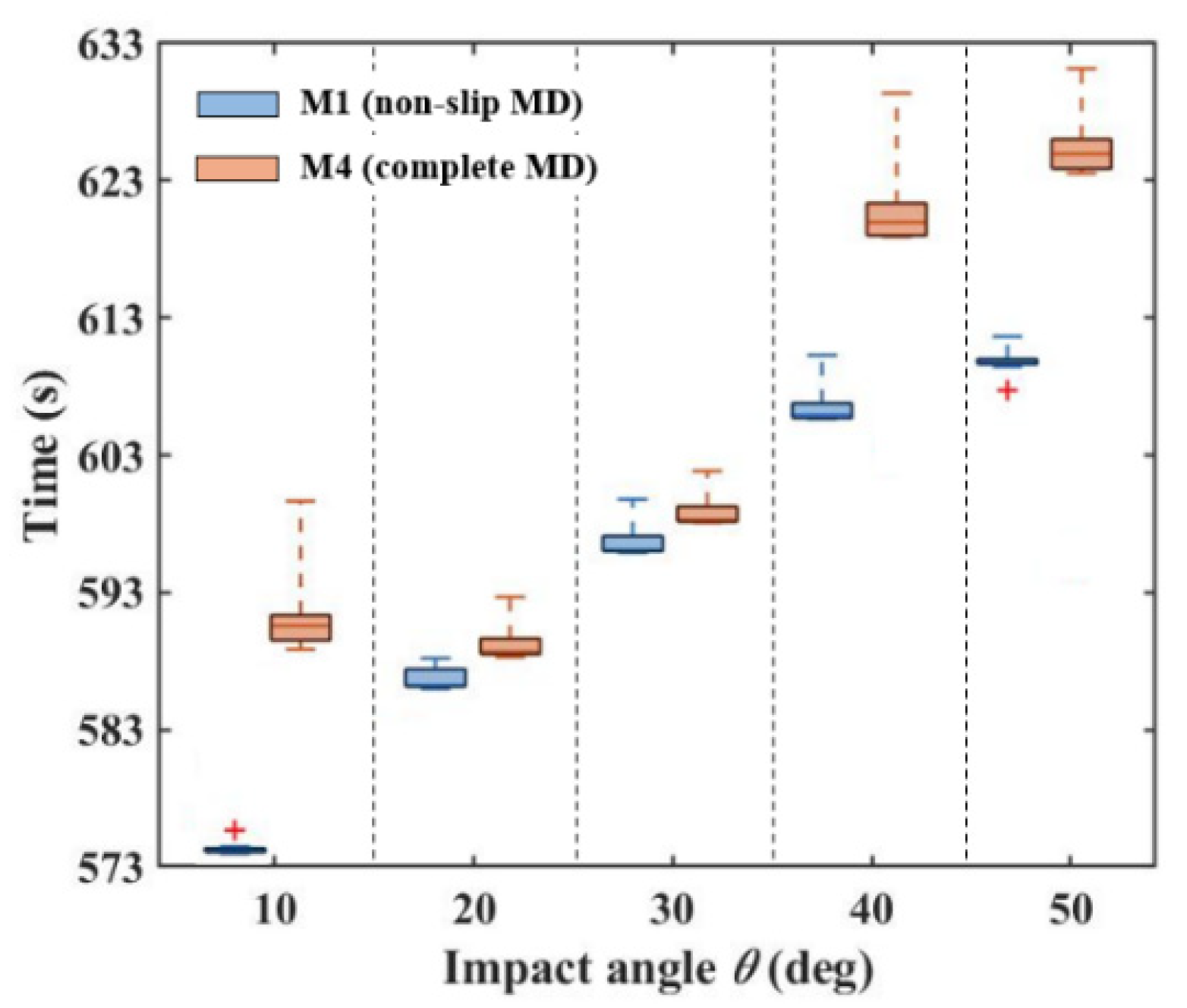
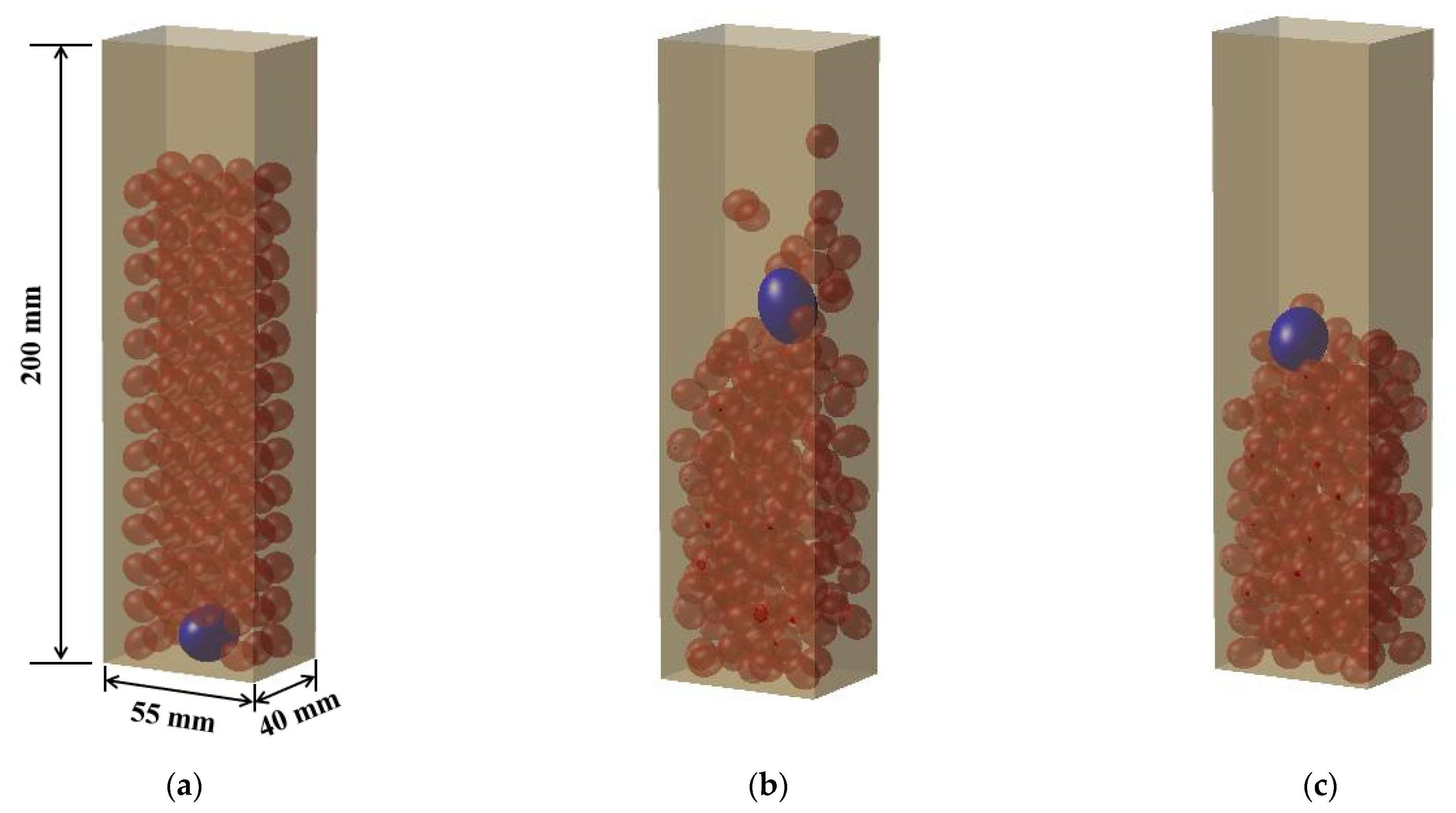
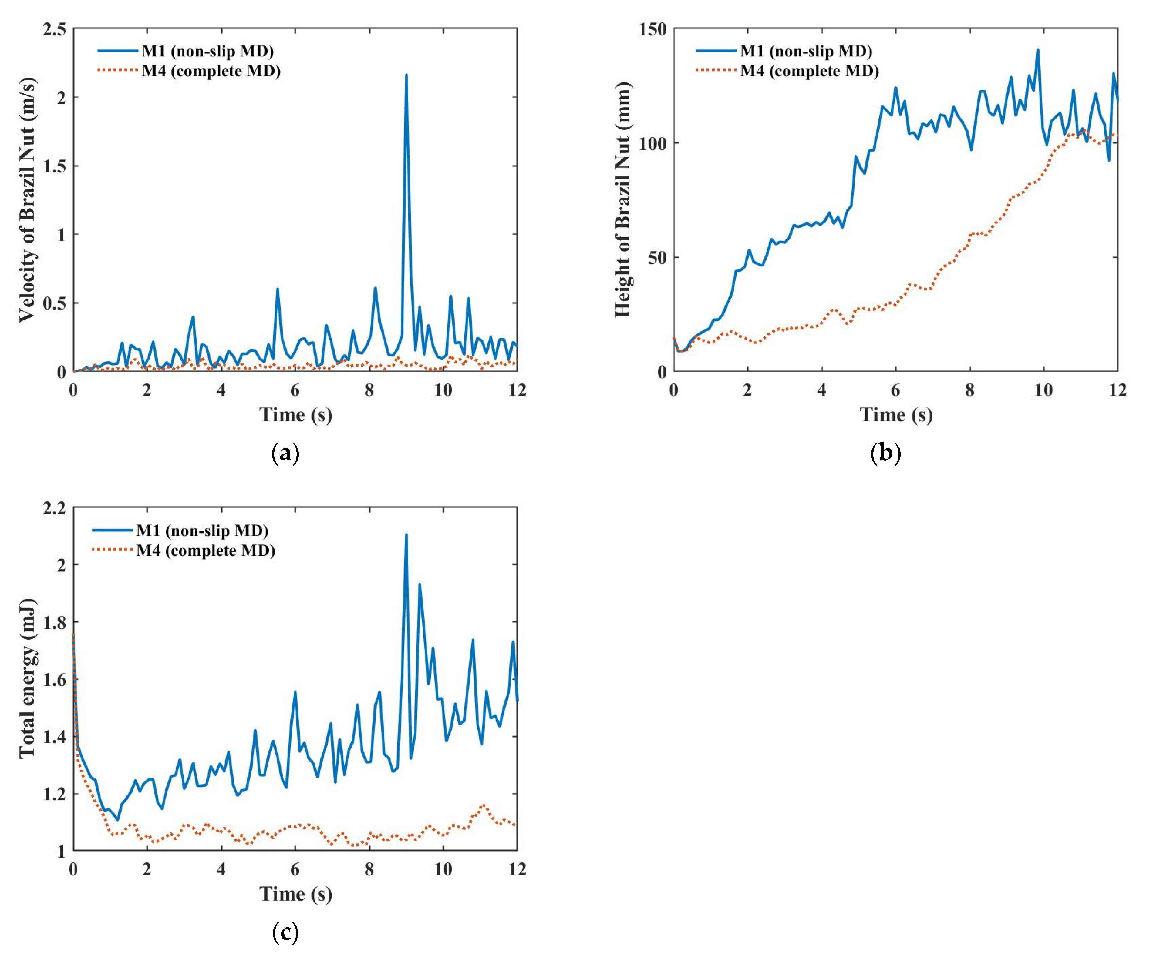
3.2. Extended Analyses Regarding the Multiple Collisions

The Brazil nut effect is applied to compare the influence of the contact force models on the multiple granular system. The Brazil nut effect describes the rise of a granule buried in an oscillating system of particles in a confined environment [53]. This study applies the ellipsoidal particles under 1 g within a cuboid box. The box rotates along the y-axis with the shacking period equaling 3 s, and the maximum rotation angle is 15°. The integral step size of the simulations is 10⁻⁵ s, satisfying Equation (24). The box’s length, width, and height are 55 mm, 40 mm, and 200 mm, respectively. In this box, 150 small ellipsoids and one larger ellipsoid are included. Their masses, sizes, and polyhedral models are listed in

Table 2. Parameters in the Brazil nut effect simulation.

Particle	Mass	Size	Vertices	Facets
Peanut	0.0019 kg	6 × 5 × 5 mm	810	1616
Brazil nut	0.012 kg	12 × 9 × 9 mm	2864	5724

, respectively. For distinction, the smaller ellipsoids are named peanut, and the larger ellipsoid is Brazil nut. The mechanical properties of the peanuts, the Brazil nut, and the box are identical, where the Young’s modulus, the Poisson ratio, and the friction coefficient are 50 Mpa, 0.2, and 0.8, respectively. The normal/tangential restitution coefficients are set identically as 0.5. Based on the above discussion in Section 3.1.2, the non-slip MD model M1 and the complete MD model M4 are applied and compared without changing the properties of the Brazil nut effect.

Figure 9 illustrates the states of these granules within four cycles (the corresponding real-time is 12 s). Figure 9a is the initial release state of the system. The blue and red ellipsoids represent the Brazil nut and peanuts, respectively (color online). Motivated by the oscillating box, the Brazil nut rises from the bottom of the box and migrates to the top gradually. Figure 9b,c are the final states after the four cycles under M1 and M4, respectively. The granules of M1 in Figure 9b are more active, with some peanuts temporarily separating from the whole particle system. The CPU calculation times of M1 and M4 are 53 h and 73 h, respectively, by applying an Intel(R) Xeon(R) Silver 4216 CPU @ 2.10 GHz. Similar to the single collision, the non-slip MD model M1 consumes a shorter CPU calculation time. In this multiple-collision case, 20 h are saved by M1, and the corresponding calculation efficiency is improved by about 27.4%. With the increase of the granule number, the computational efficiency change is more pronounced.

Figure 10 illustrates the height and velocity evolutions of the Brazil nut. The height of the Brazil nut refers to the z-axis of its position. The velocity of the Brazil nut in Figure 10a is smaller when the model M4 is applied, which is less than 0.12 m/s. However, the velocity of M1 has a maximum value exceeding 2 m/s, and the average value is around 0.19 m/s. Influenced by the larger increasing velocity of M1, the Brazil nut has arrived at the top position within 6 s in Figure 10b, which is about 4 s faster than that of M4. The average values of these granules’ total energy are illustrated in Figure 10c. The total energy refers to the sum of the kinetic and potential energy. After the initial free-falling of the granules, the external energy input of the vibrating box makes the total energies of M1 and M4 increase gradually with fluctuations. Similar to the rising velocity, the energies of M1 exceed those of M4. Additionally, when applying the model M1, the velocity, height, and energy change curves tend to have more fluctuations. This difference shows that more energies are dissipated by the damping and friction parts of M4, leading to the less intense convection phenomenon of these peanuts than M1.

Compared with the single collision, the difference between M1 and M4 becomes more significant in terms of the Brazil nut’s rising velocity, the system energy, and the CPU calculation efficiency due to the accumulation of collisions. Although the specific differences vary with the properties of the Brazil nuts, the step size, the facet number of the polyhedral model, etc., the qualitative comparison between M1 and M4 can be made. The non-slip model M1 tends to result in less energy loss in the system and significantly saves on the CPU calculation time. The calculation efficiency will be promoted by M1 more significantly with the increase of the granule number. Based on this study, more discussions about the contact force models’ differences in the non-spherical granular system are possible. For example, different Brazil nut simulations could be implemented by changing the number/size/shape of the applied granules.

4. Conclusions

This study compares the performances of four contact force models by exploiting a newly-presented discrete element method (DEM) with the Polygonal Contact Model (PCM). The four contact force models include one linear spring–dashpot model and three nonlinear models, i.e., the normal Hertzian contact with the non-slip/revised/complete forms of the tangential Mindlin–Deresiewicz model. Differences among these contact force models are presented based on the numerical simulations of the single-collision and multiple-collision scenarios.

In terms of the existing single-collision experiment, the three nonlinear contact force models have similar results in the new DEM+PCM algorithm. Compared with the complete form, the non-slip Mindlin–Deresiewicz model increases the calculation efficiency by 0.5% to 3%. Additionally, the CPU calculation efficiency is significantly increased by 93% when the softening coefficient decreases from 1 to 10⁻³. Unlimited softening turns out to be unrealistic. As for the multiple-collision case in the Brazil nut effect, the differences between the non-slip and complete Mindlin–Deresiewicz model become more striking than in the single-collision case due to numerical accumulations. The non-slip Mindlin–Deresiewicz model results in less energy dissipation and increases the computation efficiency by 27.4% in four oscillating cycles of the Brazil nut effect. Based on the above studies, the Hertzian contact with the non-slip Mindlin–Deresiewicz model is recommended in the new DEM+PCM algorithm. In future studies, the influence of the facet number of the macroscopical polyhedron on the outgoing results can be analyzed. New type(s) of contact forces among the mesoscopic elements in the DEM can be investigated as well.

References

1. Cundall, P.A.; Strack, O.D.L. A discrete numerical model for granular assemblies. Geotechnique 1979, 29, 47–65. [Google Scholar] [CrossRef]
2. Zhang, Y.; Michel, P.; Barnouin, O.S.; Roberts, J.H.; Daly, M.G.; Ballouz, R.-L.; Walsh, K.J.; Richardson, D.C.; Hartzell, C.M.; Lauretta, D.S. Inferring interiors and structural history of top-shaped asteroids from external properties of asteroid (101955) Bennu. Nat. Commun. 2022, 13, 1–12. [Google Scholar] [CrossRef]
3. Sánchez, P.; Renouf, M.; Azéma, E.; Mozul, R.; Dubois, F. A contact dynamics code implementation for the simulation of asteroid evolution and regolith in the asteroid environment. Icarus 2021, 363, 114441. [Google Scholar] [CrossRef]
4. Schwartz, S.R.; Richardson, D.C.; Michel, P. An implementation of the soft-sphere discrete element method in a high-performance parallel gravity tree-code. Gran. Matt. 2012, 14, 363–380. [Google Scholar] [CrossRef]
5. DellaGiustina, D.N.; Emery, J.P.; Golish, D.R. Properties of rubble-pile asteroid (101955) Bennu from OSIRIS-REx imaging and thermal analysis. Nat. Astron. 2019, 3, 341–351. [Google Scholar] [CrossRef] [Green Version]
6. Zhang, X.; Luo, Y.; Xiao, Y.; Liu, D.; Guo, F.; Guo, Q. Developing prototype simulants for surface materials and morphology of near earth asteroid 2016 HO3. Space Sci. Tech. 2021, 2021, 9874929. [Google Scholar] [CrossRef]
7. Huang, X.; Li, M.; Wang, X.; Hu, J.; Zhao, Y.; Guo, M.; Xu, C.; Liu, W.; Wang, Y.; Hao, C.; et al. The Tianwen-1 guidance, navigation, and control for Mars entry, descent, and landing. Space Sci. Tech. 2021, 2021, 9846185. [Google Scholar] [CrossRef]
8. Hippmann, G. An algorithm for compliant contact between complexly shaped bodies. Multibody Syst. Dyn. 2004, 12, 345–362. [Google Scholar] [CrossRef]
9. Richardson, D.C.; Walsh, K.J.; Murdoch, N.; Michel, P. Numerical simulations of granular dynamics: I. Hard-sphere discrete element method and tests. Icarus 2011, 212, 427–437. [Google Scholar] [CrossRef] [Green Version]
10. Brendel, L.; Dippel, S. Lasting contacts in molecular dynamics simulations. In Physics of Dry Granular Media, 1st ed.; Herrmann, H.J., Hovi, J.P., Luding, S., Eds.; Springer: Dordrecht, The Netherlands, 1998; Volume 350, pp. 313–318. [Google Scholar] [CrossRef]
11. García-Rojo, R.; McNamara, S.; Herrmann, H.J. Influence of Contact Modelling on the Macroscopic Plastic Response of Granular Soils Under Cyclic Loading. In Mathematical Models of Granular Matter, 1st ed.; Capriz, G., Mariano, P.M., Giovine, P., Eds.; Springer: Berlin, Heidelberg, 2008; Volume 1937, pp. 109–124. [Google Scholar] [CrossRef]
12. Brilliantov, N.V.; Spahn, F.; Hertzsch, J.M.; Pöschel, T. Model for collisions in granular gases. Phys. Rev. E 1996, 53, 5382. [Google Scholar] [CrossRef] [Green Version]
13. Tsuji, Y.; Tanaka, T.; Ishida, T. Lagrangian numerical simulation of plug flow of cohesionless particles in a horizontal pipe. Powder Technol. 1992, 71, 239–250. [Google Scholar] [CrossRef]
14. Tsuji, Y.; Kawaguchi, T.; Tanaka, T. Discrete particle simulation of two-dimensional fluidized bed. Powder Technol. 1993, 77, 79–87. [Google Scholar] [CrossRef]
15. Mindlin, R.D. Compliance of elastic bodies in contact. J. Appl. Mech. 1949, 16, 259–268. [Google Scholar] [CrossRef]
16. Mindlin, R.D.; Deresiewicz, H. Elastic spheres in contact under varying oblique forces. J. Appl. Mech. 1953, 20, 327–344. [Google Scholar] [CrossRef]
17. Maw, N.; Barber, J.R.; Fawcett, J.N. The oblique impact of elastic spheres. Wear 1976, 38, 101–114. [Google Scholar] [CrossRef]
18. Maw, N.; Barber, J.R.; Fawcett, J.N. The role of elastic tangential compliance in oblique impact. J. Lubr. Technol. 1981, 103, 74–80. [Google Scholar] [CrossRef]
19. Walton, O.R.; Braun, R.L. Viscosity, granular-temperature, and stress calculations for shearing assemblies of inelastic, frictional disks. J. Rheol. 1986, 30, 949–980. [Google Scholar] [CrossRef]
20. Kruggel-Emden, H.; Wirtz, S.; Scherer, V. A study on tangential force laws applicable to the discrete element method (DEM) for materials with viscoelastic or plastic behavior. Chem. Eng. Sci. 2008, 63, 1523–1541. [Google Scholar] [CrossRef]
21. Zhong, W.; Yu, A.; Liu, X.; Tong, Z.; Zhang, H. DEM/CFD-DEM modeling of non-spherical particulate systems: Theoretical developments and applications. Powder Technol. 2016, 302, 108–152. [Google Scholar] [CrossRef]
22. Richardson, D.C.; Quinn, T.; Stadel, J.; Lake, G. Direct large-scale N-body simulations of planetesimal dynamics. Icarus 2000, 143, 45–59. [Google Scholar] [CrossRef] [Green Version]
23. Cheng, B.; Yu, Y.; Baoyin, H. Collision-based understanding of the force law in granular impact dynamics. Phys. Rev. E 2018, 98, 012901. [Google Scholar] [CrossRef]
24. Liu, C.; Pollard, D.D.; Shi, B. Analytical Solutions and Numerical Tests of Elastic and Failure Behaviors of Close-Packed Lattice for Brittle Rocks and Crystals. J. Geophys. Res. Solid Earth 2013, 118, 71–82. [Google Scholar] [CrossRef]
25. Murdoch, N.; Drilleau, M.; Sunday, C.; Thuillet, F.; Wilhelm, A.; Nguyen, G.; Gourinat, Y. Low-velocity impacts into granular material: Application to small-body landing. Mon. Not. R. Astron. Soc. 2021, 503, 3460–3471. [Google Scholar] [CrossRef]
26. Cheng, B.; Yu, Y.; Asphaug, E.; Michel, P.; Richardson, D.C.; Hirabayashi, M.; Yoshikawa, M.; Baoyin, H. Reconstructing the formation history of top-shaped asteroids from the surface boulder distribution. Nat. Astron. 2021, 5, 134–138. [Google Scholar] [CrossRef]
27. Raducan, S.D.; Jutzi, M.; Zhang, Y.; Ormö, J.; Michel, P. Reshaping and ejection processes on rubble-pile asteroids from impacts. Astron. Astrophys. 2022, 665, L10. [Google Scholar] [CrossRef]
28. Kruggel-Emden, H.; Wirtz, S.; Scherer, V. Applicable contact force models for the discrete element method: The single particle perspective. J. Press. Vessel Technol. 2009, 131, 024001. [Google Scholar] [CrossRef]
29. Gorham, D.A.; Kharaz, A.H. The measurement of particle rebound characteristics. Powder Technol. 2000, 112, 193–202. [Google Scholar] [CrossRef]
30. Zhang, Y.; Li, J.; Zeng, Z.; Wen, T.; Li, Z. High-fidelity landing simulation of small body landers: Modeling and mass distribution effects on bouncing motion. Aerosp. Sci. Technol. 2021, 119, 107149. [Google Scholar] [CrossRef]
31. Zeng, X.; Wen, T.; Li, Z.; Alfriend, K.T. Natural Landing Simulations on Generated Local Rocky Terrains for Asteroid Cubic Lander. IEEE Trans. Aerosp. Electron. Syst. 2022, 58, 3492–3508. [Google Scholar] [CrossRef]
32. Wen, T.; Zeng, X.; Circi, C.; Gao, Y. Hop reachable domain on irregularly shaped asteroids. J. Guid. Control Dyn. 2020, 43, 1269–1283. [Google Scholar] [CrossRef]
33. Zeng, X.; Li, Z.; Wen, T.; Zhang, Y. Influence of the lander size and shape on the ballistic landing motion. Earth Space Sci. 2022, 9, e2021EA001952. [Google Scholar] [CrossRef]
34. Ebrahimi, S.; Hippmann, G.; Eberhard, P. Extension of the polygonal contact model for flexible multibody systems. Int. J. Appl. Math. Mech. 2005, 1, 33–50. [Google Scholar]
35. Zeng, X.; Wen, T.; Yu, Y.; Cheng, B.; Qiao, D. New practical discrete non-spherical N-body method: Validation with the Brazil nut effect. Icarus 2022, 387, 115201. [Google Scholar] [CrossRef]
36. Wen, T.; Zeng, X.; Li, Z.; Zhang, Y. Size segregation of non-spherical particles under different gravity levels. Planet. Space Sci. 2022; submitted. [Google Scholar]
37. Serra-Aguila, A.; Puigoriol-Forcada, J.M.; Reyes, G.; Menacho, J. Viscoelastic models revisited: Characteristics and interconversion formulas for generalized Kelvin-Voigt and Maxwell models. Acta Mech. Sin. 2019, 35, 1191–1209. [Google Scholar] [CrossRef]
38. Vu-Quoc, L.; Zhang, X. An accurate and efficient tangential force-displacement model for elastic frictional contact in particle-flow simulations. Mech. Mater. 1999, 31, 235–269. [Google Scholar] [CrossRef]
39. Hunt, K.H.; Crossley, F.R.E. Coefficient of Restitution Interpreted as Damping in Vibroimpact. J. Appl. Mech. 1975, 42, 440. [Google Scholar] [CrossRef]
40. Wada, K.; Senshu, H.; Matsui, T. Numerical simulation of impact cratering on granular material. Icarus 2006, 180, 528–545. [Google Scholar] [CrossRef]
41. Cheng, B.; Asphaug, E.; Yu, Y.; Baoyin, H. Measuring the mechanical properties of small body regolith layers using a granular penetrometer. Astrodynamics 2023, 7, 15–29. [Google Scholar] [CrossRef]
42. Antypov, D.; Elliott, J.A. On an analytical solution for the damped Hertzian spring. Europhys. Lett. 2011, 94, 50004. [Google Scholar] [CrossRef]
43. Hu, G. Analysis and Simulation of Granular System by Discrete Element Method Using EDEM, 1st ed.; Wuhan University of Technology Press: Wuhan, China, 2010; pp. 12–15. [Google Scholar]
44. Di Renzo, A.; Di Maio, F.P. An improved integral non-linear model for the contact of particles in distinct element simulations. Chem. Eng. Sci. 2005, 60, 1303–1312. [Google Scholar] [CrossRef]
45. Di Renzo, A.; Di Maio, F.P. Comparison of contact-force models for the simulation of collisions in DEM-based granular flow codes. Chem. Eng. Sci. 2004, 59, 525–541. [Google Scholar] [CrossRef]
46. Thornton, C.; Cummins, S.J.; Cleary, P.W. An investigation of the comparative behaviour of alternative contact force models during inelastic collisions. Powder Technol. 2013, 233, 30–46. [Google Scholar] [CrossRef]
47. Thornton, C.; Cummins, S.J.; Cleary, P.W. An investigation of the comparative behaviour of alternative contact force models during elastic collisions. Powder Technol. 2011, 210, 189–197. [Google Scholar] [CrossRef]
48. Kharaz, A.H.; Gorham, D.A.; Salman, A.D. An experimental study of the elastic rebound of spheres. Powder Technol. 2001, 120, 281–291. [Google Scholar] [CrossRef]
49. Džiugys, A.; Peters, B. An approach to simulate the motion of spherical and non-spherical fuel particles in combustion chambers. Gran. Matt. 2001, 3, 231–266. [Google Scholar] [CrossRef]
50. Cheng, B. Granular Dynamics for Small Body Touchdown Missions. Ph.D. Thesis, Tsinghua University, Beijing, China, 2021. [Google Scholar]
51. Sun, Q.; Wang, G. Introduction to Mechanics of Granular Matter, 1st ed.; Science Press: Beijing, China, 2009; pp. 162–163. [Google Scholar]
52. Hoomans, B. Granular Dynamics of Gas Solid Two Phase Flows. Ph.D. Thesis, Universiteit Twente, Enschede, The Netherlands, 2000. [Google Scholar]
53. Perera, V.; Jackson, A.P.; Asphaug, E.; Ballouz, R.-L. The spherical Brazil Nut Effect and its significance to asteroids. Icarus 2016, 278, 194–203. [Google Scholar] [CrossRef]
Figure 1. Process of the complete MD model when the displacements increase.
Aerospace 09 00737 g001
Figure 2. Loading comparison between three different MD models.
Aerospace 09 00737 g002
Figure 3. Illustration of the single-collision experiment. (a) oblique ingoing velocity; (b) rotation of the plane.
Aerospace 09 00737 g003
Figure 4. Comparison between the experiment and the simulation results. (a) restitution coefficient; (b) outgoing angular velocity; (c) rebound angle; (d) non-dimensional angle; (e) energy.
Aerospace 09 00737 g004
Figure 5. Deviation comparison between the four contact force models. (a) deviation of en; (b) deviation of et; (c) deviation of ωout; (d) deviation of αv; (e) deviation of αc; (f) deviation of Eout.
Aerospace 09 00737 g005aAerospace 09 00737 g005b
Figure 6. Comparison of the tangential forces by applying the nonlinear models. (a) tangential force; (b) static tangential force.
Aerospace 09 00737 g006
Figure 7. Comparison of the CPU calculation times of M1 and M4.
Aerospace 09 00737 g007
Figure 8. Comparison of the softening simulations. (a) normal restitution coefficient; (b) tangential restitution coefficient; (c) outgoing angular velocity; (d) rebound angle; (e) translational energy; (f) rotational energy.
Aerospace 09 00737 g008aAerospace 09 00737 g008b
Figure 9. States of the Brazil nut effect. (a) initial state; (b) final state under M1; (c) final state under M4.
Aerospace 09 00737 g009
Figure 10. Comparison between M1 and M4 by applying the Brazil nut effect. (a) velocity of the Brazil nut; (b) height of the Brazil nut; (c) total energy.
Aerospace 09 00737 g010