
Stability of a Flexible Asteroid Lander with Landing Control


Abstract
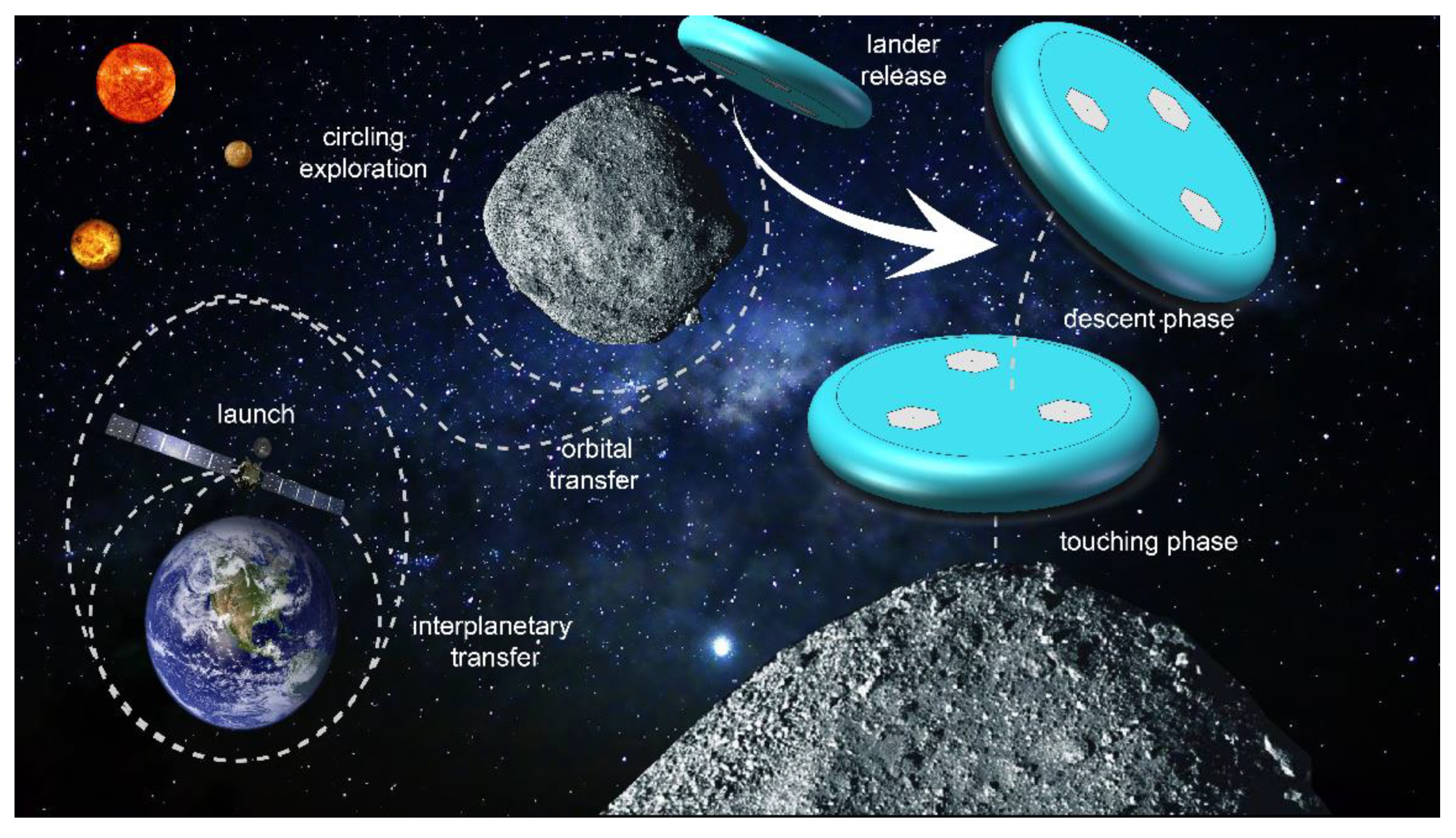
:1. Introduction
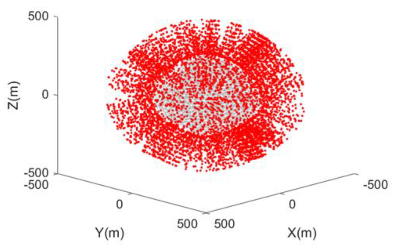
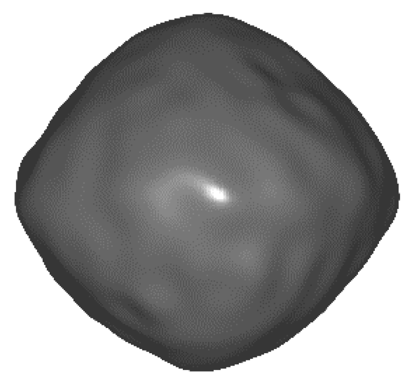
2. Asteroid’s Dynamical Environment
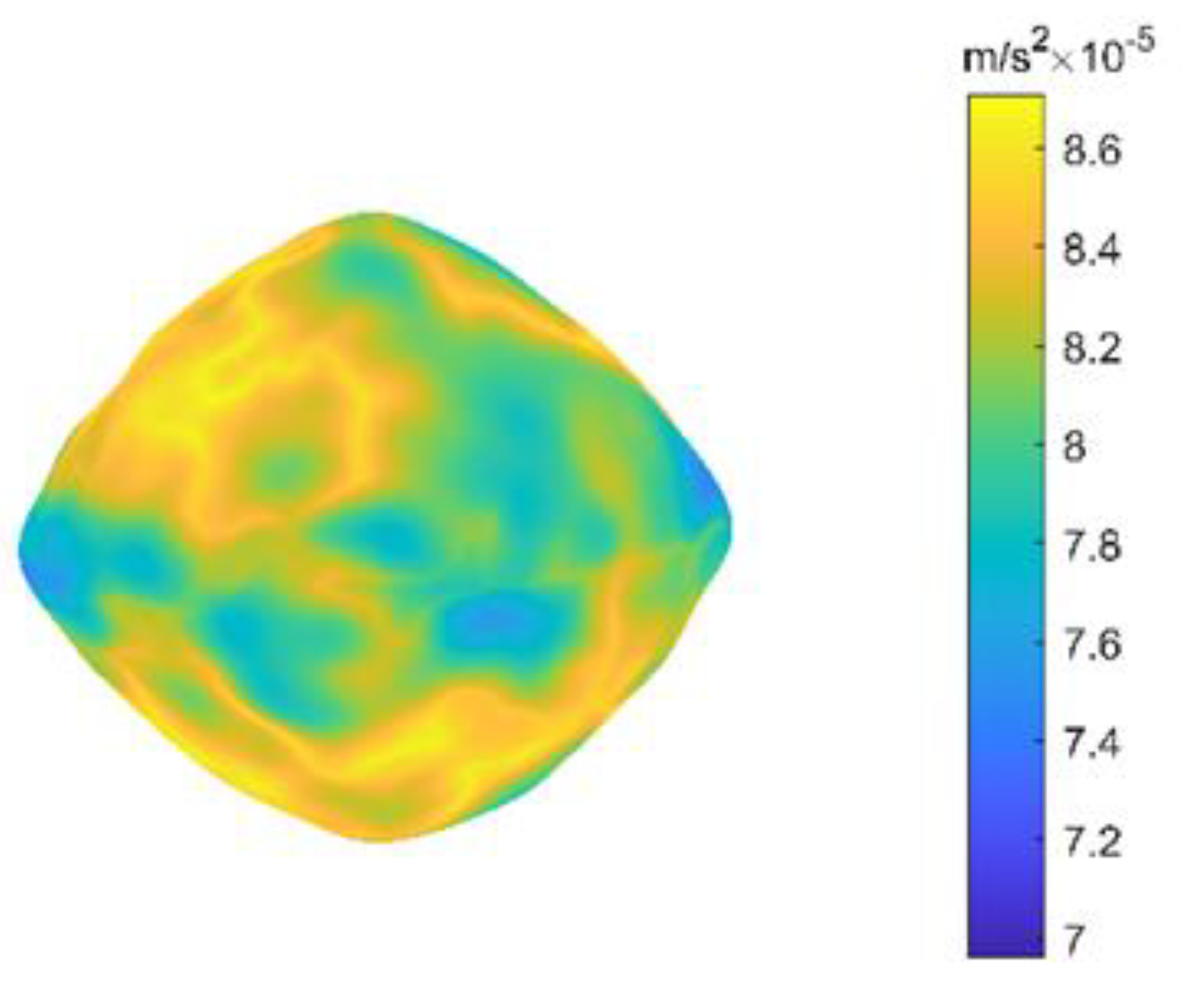
2.1. Gravity Model
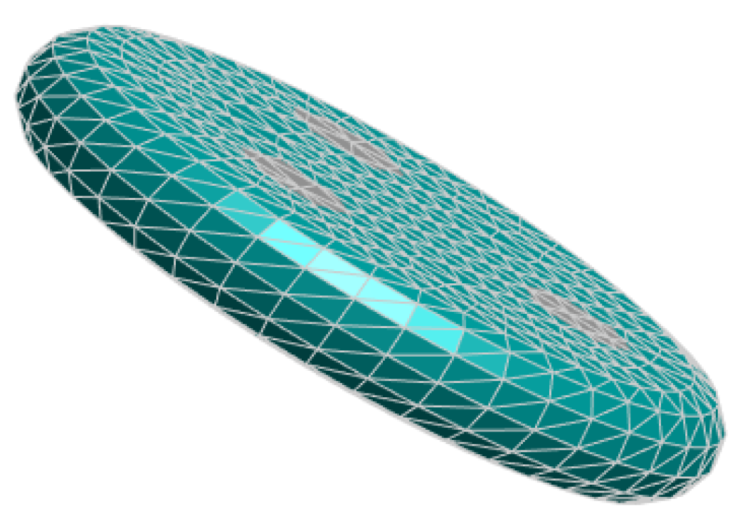
2.2. Surface Model
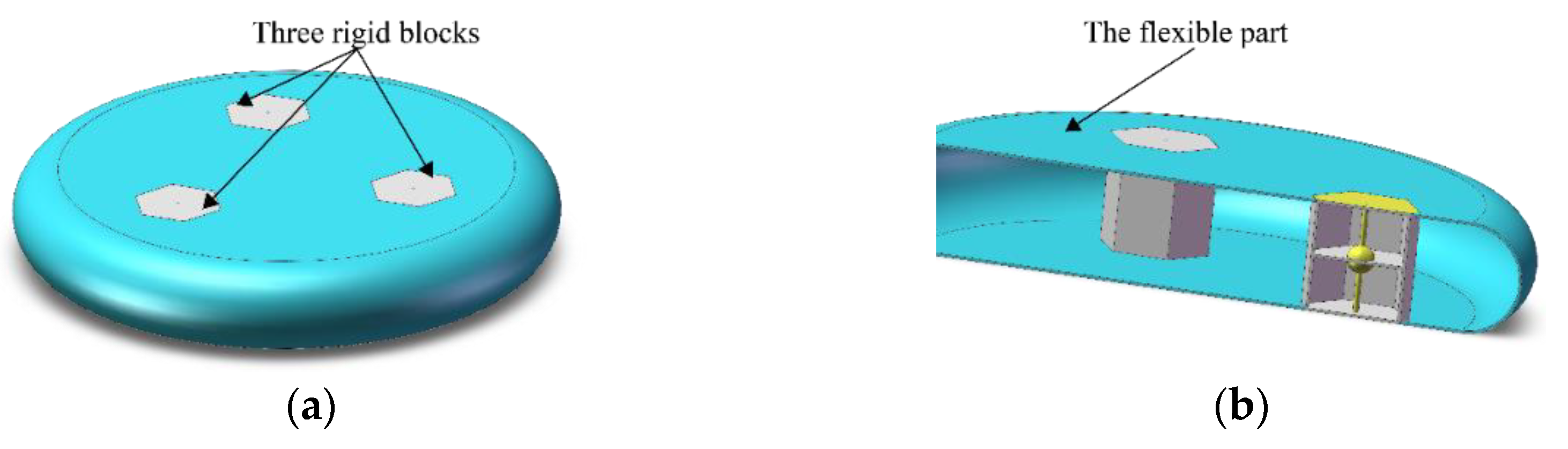
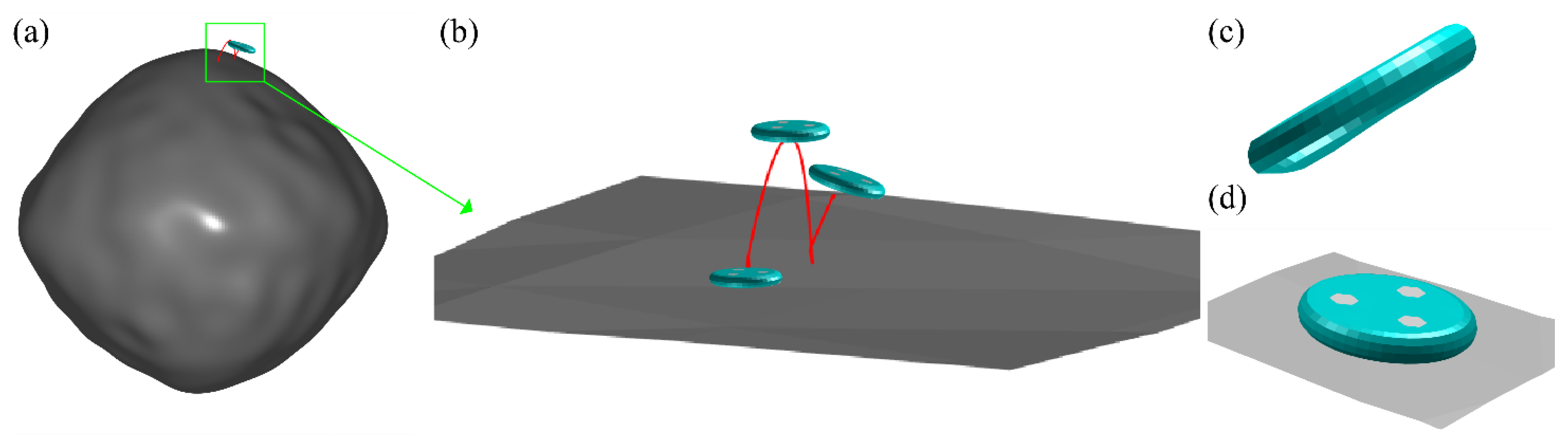
3. Flexible Landing Dynamics
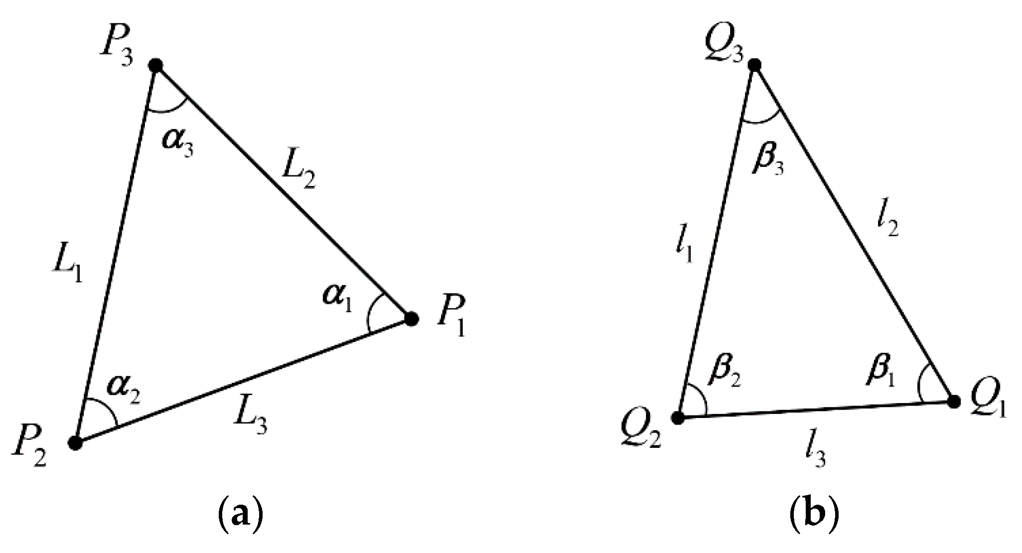
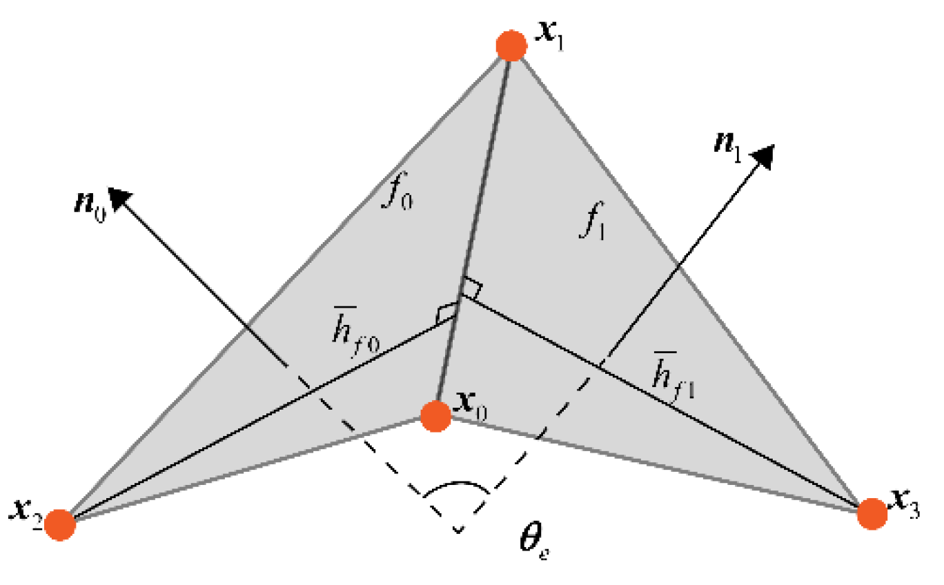
3.1. Dynamics of the Flexible Part
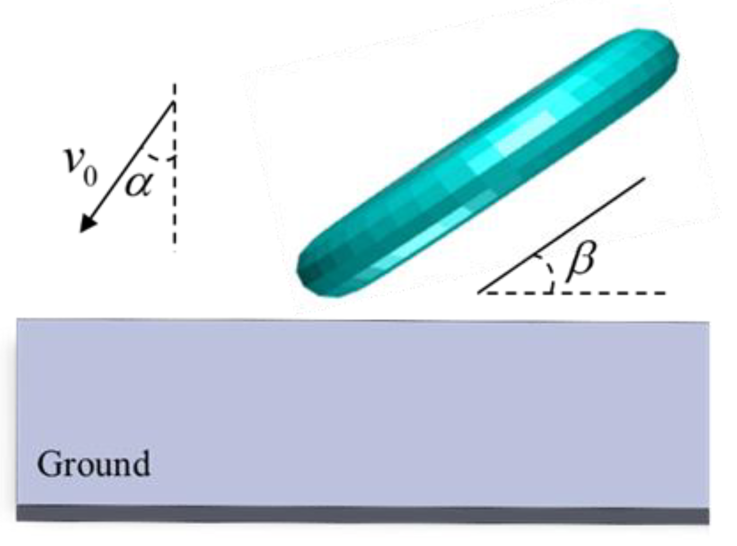
3.2. Collision Model
3.3. Coupling Dynamics
4. Control Scheme for the Descent Phase
4.1. Attitude Control
4.2. Position Control
5. Landing Simulation and Discussions
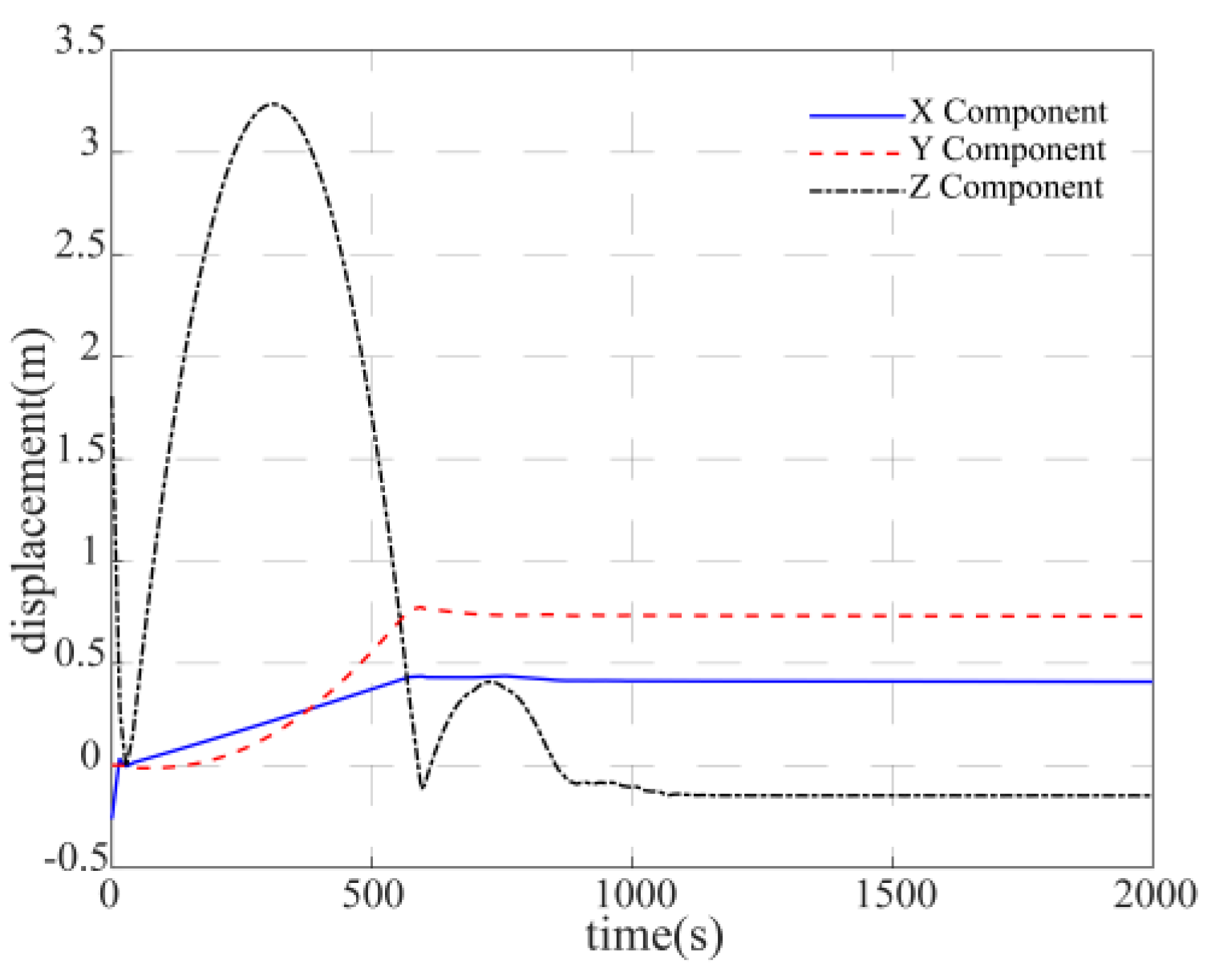
5.1. Stable Landing Scenario
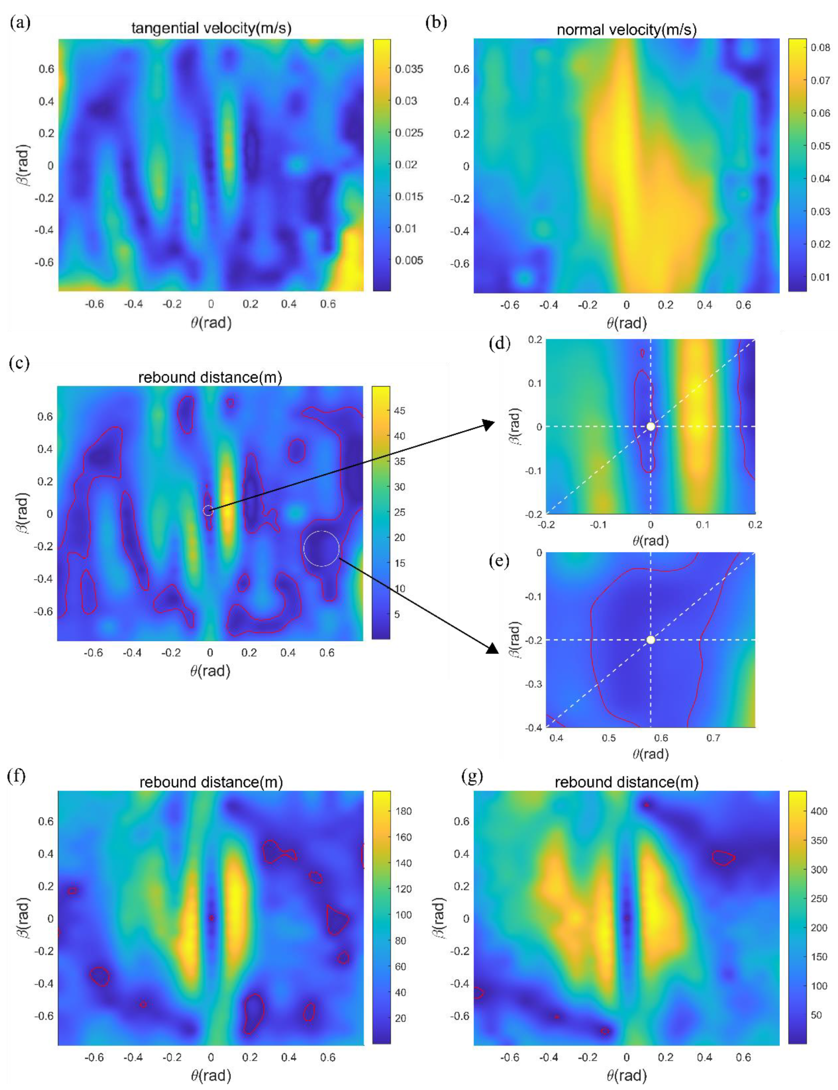
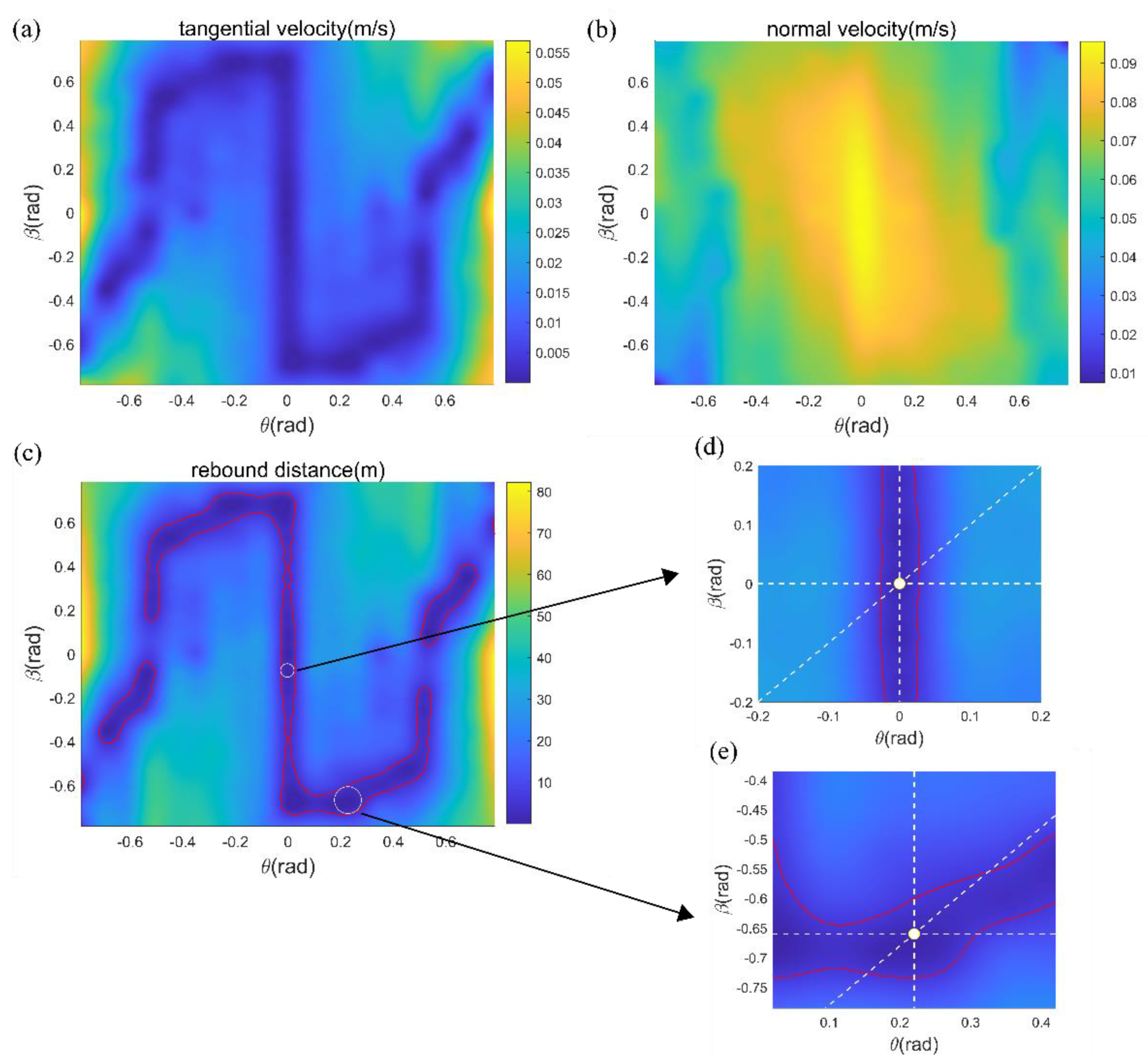
5.2. Landing Stability of the Flexible Lander
5.3. Comparison with the Rigid Lander
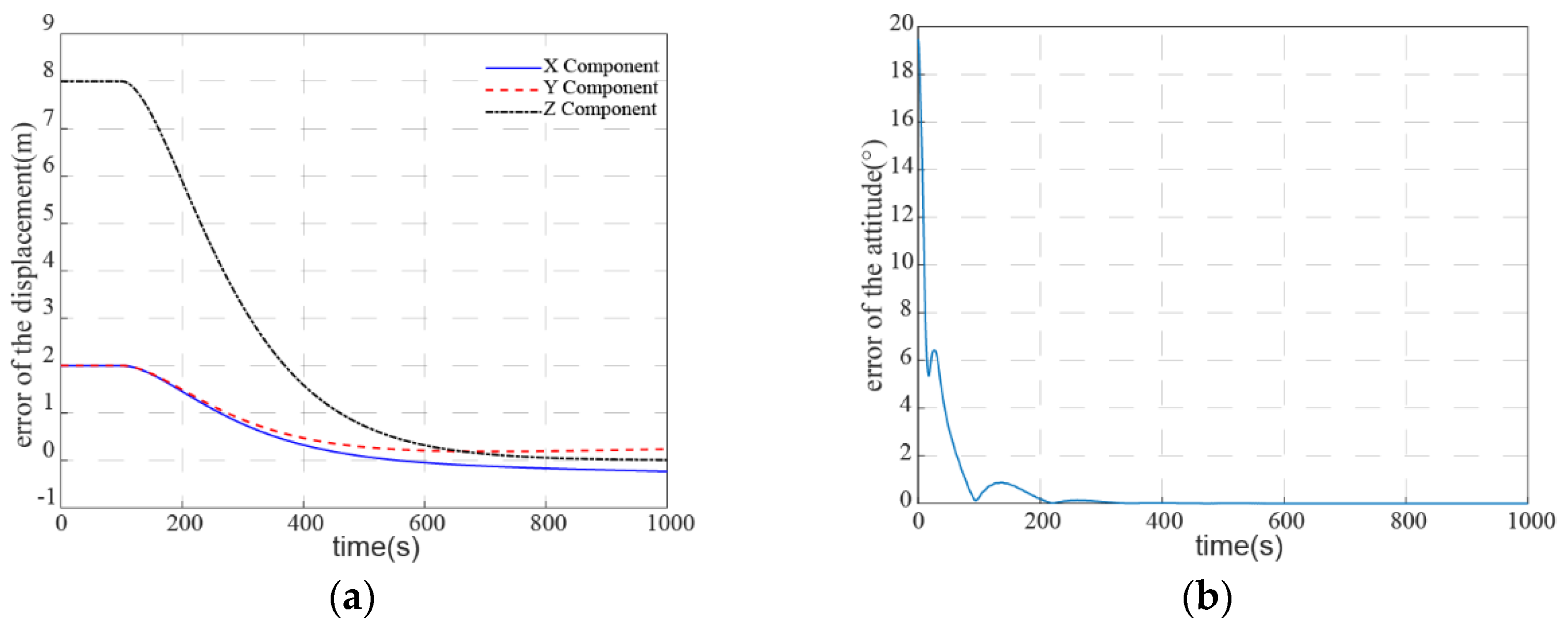
5.4. Simulation of the Descent Phase
6. Conclusions
Author Contributions
Funding
Institutional Review Board Statement
Informed Consent Statement
Data Availability Statement
Conflicts of Interest
References
- Castillo-Rogez, J.C.; Pavone, M.; Nesnas, I.; Hoffman, J.A. Expected science return of spatially-extended in-situ exploration at small Solar system bodies. In Proceedings of the Aerospace Conference, Big Sky, MT, USA, 3–10 March 2012. [Google Scholar]
- Peloni, A.; Ceriotti, M.; Dachwald, B. Solar-Sail Trajectory Design for a Multiple Near-Earth-Asteroid Rendezvous Mission. J. Guid. Control Dyn. A Publ. Am. Inst. Aeronaut. Astronaut. Devoted Technol. Dyn. Control 2016, 39, 2712–2724. [Google Scholar] [CrossRef] [Green Version]
- Luo, Y.; Jiang, X.; Zhong, S.; Ji, Y.; Sun, G. Multisatellite Task Allocation and Orbit Planning for Asteroid Terminal Defence. Aerospace 2022, 9, 364. [Google Scholar] [CrossRef]
- Yan, W.; Baoyin, H. A Numerical Research on a New Type of Asteroid Flexible Probe. IEEE Access 2021, 9, 129863–129873. [Google Scholar] [CrossRef]
- Dorofeeva, V.A. Chemical and Isotope Composition of Comet 67P/ChuryumovGerasimenko: The RosettaPhilae Mission Results Reviewed in the Context of Cosmogony and Cosmochemistry. Sol. Syst. Res. 2020, 54, 96–120. [Google Scholar] [CrossRef]
- Hand, E. Philae probe makes bumpy touchdown on a comet. Science 2014, 346, 900–901. [Google Scholar] [CrossRef]
- Yoshikawa, M.; Kawaguchi, J.; Kuninaka, H. The Results of Asteroid Exploration Mission Hayabusa. Ieice Tech. Rep. 2010, 110, 219–222. [Google Scholar]
- Fujiwara, A.; Kawaguchi, J.; Yeomans, D.; Abe, M.; Mukai, T.; Okada, T.; Saito, J.; Yano, H.; Yoshikawa, M.; Scheeres, D. The rubble-pile asteroid Itokawa as observed by Hayabusa. Science 2006, 312, 1330–1334. [Google Scholar] [CrossRef]
- Li, X.; Qiao, D.; Huang, J.; Han, H.; Meng, L. Dynamics and control of proximity operations for asteroid exploration mission. Sci. China Phys. Mech. Astron. 2019, 49, 084508. (In Chinese) [Google Scholar] [CrossRef]
- Tang, G.; Jiang, F.; Li, J. Low-thrust trajectory optimization of asteroid sample return mission with multiple revolutions and moon gravity assists. Sci. China Phys. Mech. Astron. 2015, 58, 114501. [Google Scholar] [CrossRef]
- Chen, Y.; Baoyin, H.; Li, J. Design and optimization of a trajectory for Moon departure Near Earth Asteroid exploration. Sci. China Phys. Mech. Astron. 2011, 54, 748–755. [Google Scholar] [CrossRef]
- Huang, J.; Li, X.; Qiao, D.; Jia, F.; Meng, L. Mission design for multi-target and multi-mode rendezvous missions to small bodies. Sci. China Phys. Mech. Astron. 2019, 49, 084512. (In Chinese) [Google Scholar] [CrossRef]
- Wal, S.V.; Reid, R.G.; Scheeres, D.J. Simulation of Nonspherical Asteroid Landers: Contact Modeling and Shape Effects on Bouncing. J. Spacecr. Rocket. 2019, 57, 1–22. [Google Scholar]
- Bazzocchi, M.C.; Hakima, H. A CubeSat-based Robotic Asteroid Sampling Mission. In Proceedings of the AIAA Scitech 2020 Forum, Orlando, FL, USA, 6–10 January 2020. [Google Scholar]
- Kim, Y.-B.; Jeong, H.-J.; Park, S.-M.; Lim, J.H.; Lee, H.-H. Prediction and Validation of Landing Stability of a Lunar Lander by a Classification Map Based on Touchdown Landing Dynamics’ Simulation Considering Soft Ground. Aerospace 2021, 8, 380. [Google Scholar] [CrossRef]
- Zhang, Y.; Li, J.; Zeng, X.; Wen, T.; Li, Z. High-fidelity landing simulation of small body landers: Modeling and mass distribution effects on bouncing motion. Aerosp. Sci. Technol. 2021, 119, 107149. [Google Scholar] [CrossRef]
- Wen, T.; Zeng, X.; Circi, C.; Gao, Y. Hop reachable domain on irregularly shaped asteroids. J. Guid. Control Dyn. 2020, 43, 1269–1283. [Google Scholar] [CrossRef]
- Zen, X.; Li, Z.; Gan, Q.; Circi, C. Numerical study on the low-velocity impact of the asteroid lander onto deformable regolith surfaces. J. Guid. Control Dyn. 2022, 45, 1644–1660. [Google Scholar]
- Zhao, Z.; Zhao, J.; Hong, L. An asteroid landing mechanism and its landing simulation. In Proceedings of the 2012 IEEE International Conference on Robotics and Biomimetics (ROBIO), Guangzhou, China, 11–14 December 2012. [Google Scholar]
- Wang, Y.; Jiang, W.; Long, L.; Zhu, Q.; Feng, R.; Wang, L.; Antonio, C. Design and Experimental Research of a New Type of Asteroid Anchoring System. Int. J. Aerosp. Eng. 2021, 2021, 1–7. [Google Scholar]
- Zhang, Y.; Yu, Y.; Baoyin, H. Dynamical behavior of flexible net spacecraft for landing on asteroid. Astrodynamics 2021, 5, 249–261. [Google Scholar] [CrossRef]
- Bartlett, N.W.; Tolley, M.T.; Overvelde, J.T.B.; Weaver, J.C.; Mosadegh, B.; Bertoldi, K.; Whitesides, G.M.; Wood, R.J. A 3D-printed, functionally graded soft robot powered by combustion. Science 2015, 349, 161–165. [Google Scholar] [CrossRef] [Green Version]
- Feng, R.; Zhang, Y.; Liu, J.; Zhang, Y.; Li, J.; Baoyin, H. Soft Robotic Perspective and Concept for Planetary Small Body Exploration. Soft Robot. 2022, 9, 889–899. [Google Scholar] [CrossRef]
- Hamilton, D.P.; Burns, J.A. Orbital stability zones about asteroids. Icarus 1991, 92, 118–131. [Google Scholar] [CrossRef] [Green Version]
- Werner, R.A.; Scheeres, D.J. Exterior gravitation of a polyhedron derived and compared with harmonic and mascon gravitation representations of asteroid 4769 Castalia. Celest. Mech. Dyn. Astron. 1996, 65, 313–344. [Google Scholar] [CrossRef]
- Song, Y.; Cheng, L.; Gong, S. Fast estimation of gravitational field of irregular asteroids based on deep learning and its applications. In Proceedings of the 29th AAS/AIAA Space Flight Mechanics Meeting, Maui, HI, USA, 13–17 January 2019. [Google Scholar]
- Chesley, S.R.; Farnocchia, D.; Nolan, M.C.; Vokrouhlický, D.; Chodas, P.W.; Milani, A.; Spoto, F.; Rozitis, B.; Benner, L.A.; Bottke, W.F.; et al. Orbit and bulk density of the OSIRIS-REx target Asteroid (101955) Bennu. Icarus 2014, 235, 5–22. [Google Scholar] [CrossRef] [Green Version]
- Yu, Y.; Michel, P.; Hirabayashi, M.; Schwartz, S.R.; Zhang, Y.; Richardson, D.C.; Liu, X. The Dynamical Complexity of Surface Mass Shedding from a Top-shaped Asteroid Near the Critical Spin Limit. Astron. J. 2018, 156, 59. [Google Scholar] [CrossRef]
- Grinspun, E. A Discrete Model of Thin Shells; Birkhäuser: Basel, Switzerland, 2005. [Google Scholar]
- Wardetzky, M.; Bergou, M.; Harmon, D.; Zorin, D.; Grinspun, E. Discrete quadratic curvature energies. Comput. Aided Geom. Des. 2007, 24, 499–518. [Google Scholar] [CrossRef]
- Delingette, H. Triangular Springs for Modeling Nonlinear Membranes. IEEE Trans. Vis. Comput. Graph. 2008, 14, 329–341. [Google Scholar] [CrossRef]
- Mohamed, A.-N.A.; Shabana, A.A. A nonlinear visco-elastic constitutive model for large rotation finite element formulations. Multibody Syst. Dyn. 2011, 26, 57–79. [Google Scholar] [CrossRef]
- Shan, M.; Guo, J.; Gill, E. Contact dynamic models of space debris capturing using a net. Acta Astronaut. 2017, 158, 198–205. [Google Scholar] [CrossRef]
- Zhang, F.; Huang, P.; Meng, Z.; Zhang, Y.; Liu, Z. Dynamics Analysis and Controller Design for Maneuverable Tethered Space Net Robot. J. Guid. Control Dyn. 2017, 40, 1–16. [Google Scholar] [CrossRef]
- Si, J. Dynamics Modeling and Simulation of a Net Closing Mechanism for Tether-Net Capture. Int. J. Aerosp. Eng. 2021, 2021, 1–16. [Google Scholar] [CrossRef]
- Baumgarte, J.W. A New Method of Stabilization for Holonomic Constraints. J. Appl. Mech. 1983, 50, 869. [Google Scholar] [CrossRef]
- Liu, Y. Advanced Dynamics; Academic: Beijing, China, 2003; p. 113. [Google Scholar]
- Chiou, J.C.; Wu, S.D.; Wit, S.D. Constraint violation stabilization using input-output feedback linearization in multibody dynamic analysis. In Proceedings of the Guidance, Navigation, and Control Conference, San Diego, CA, USA, 29–31 July 1996. [Google Scholar]
- Mueller, M.W.; D’Andrea, R. Stability and control of a quadrocopter despite the complete loss of one, two, or three propellers. In Proceedings of the 2014 IEEE International Conference on Robotics and Automation (ICRA), Hong Kong, China, 31 May–7 June 2014. [Google Scholar]
- Tuna, S.E. LQR-Based Coupling Gain for Synchronization of Linear Systems. arXiv 2008, arXiv:0801.3390. [Google Scholar]


Publisher’s Note: MDPI stays neutral with regard to jurisdictional claims in published maps and institutional affiliations. |
© 2022 by the authors. Licensee MDPI, Basel, Switzerland. This article is an open access article distributed under the terms and conditions of the Creative Commons Attribution (CC BY) license (https://creativecommons.org/licenses/by/4.0/).
Share and Cite
Yan, W.; Feng, R.; Baoyin, H. Stability of a Flexible Asteroid Lander with Landing Control. Aerospace 2022, 9, 719. https://doi.org/10.3390/aerospace9110719
Yan W, Feng R, Baoyin H. Stability of a Flexible Asteroid Lander with Landing Control. Aerospace. 2022; 9(11):719. https://doi.org/10.3390/aerospace9110719
Chicago/Turabian StyleYan, Weifeng, Ruoyu Feng, and Hexi Baoyin. 2022. "Stability of a Flexible Asteroid Lander with Landing Control" Aerospace 9, no. 11: 719. https://doi.org/10.3390/aerospace9110719