1. Introduction
Asteroids are terrestrial bodies mainly in the Main Asteroid Belt of our Solar System, primarily located between Mars and Jupiter. The Asteroid Belt (~2.1–3.3 au) is estimated to have about
bodies with a diameter greater than about 1 km [
1,
2]. Scientists can learn about the origin and evolution of our solar system by studying the geophysics and geochemistry of asteroids. Vesta is the second-largest asteroid and, supposedly, the parent body of meteorites in the Main Asteroid Belt. Coradini et al. [
3] theorized that the thermal evolution of Vesta took place at a time contemporary to the formation of Jupiter. There is an assumption that HED (Howardites, Eucrites, and Diogenites) meteorites found on Earth originated from Vesta [
4].
Vesta was the fourth body discovered in the Main Asteroid Belt in 1807; observations from NASA’s Hubble Space Telescopes reveal some hints of its surface composition. In recent decades, an increasing number of missions were designed to explore the asteroids in the solar system, including the sample return missions, the OSIRIS-REx (2016) [
5] to asteroid Bennu mission, and the Hayabusa2 (2014) [
6,
7] to asteroid Ryugu mission. The most well-known mission to Vesta is NASA’s Dawn mission [
8,
9], which was launched on 27 September 2007 and finally entered an orbit around Vesta in July 2011. The spacecraft spent 14 months in a series of orbits of different Vesta altitudes, studying the surface and probing the interior through gravity measurements [
10]. Dawn’s observation of Vesta reveals that the surface is dominated by variously sized impact craters [
11,
12] at a survey orbit altitude of ~2700 km. The gravity field was investigated based on collected data from the Deep Space Network Doppler tracking and optical landmark images [
13].
In the past few years, much research on various special spacecraft orbits around planets has been conducted, especially on spacecraft orbits of Earth, Mars, and Jupiter [
14,
15,
16,
17,
18,
19,
20]. Usually, these special orbits include stationary orbits, frozen orbits, Sun-synchronous orbits, repeating ground-track orbits, and orbits at the critical inclination. Li et al. [
21] proposed an analytic method for frozen orbit design and discussed the properties of frozen orbits around Vesta. Since an asteroid usually has a body with an irregular shape, its gravity field is very different from Earth. Werner et al. [
22] introduced a polyhedral method to evaluate the gravitation of irregularly shaped bodies, but the integration is computationally demanding. Moreover, many researchers have conducted much work on equilibrium points of irregularly shaped asteroids [
23,
24,
25,
26,
27]. Although the harmonic expansions of the gravitational field are always an approximation to reality, the series can be truncated at a limited order to obtain accuracy in modeling. As far as is known, there are few studies about orbits around Vesta using the mean element theory. This paper aims to investigate the existence and control of special orbits around Vesta and mainly considers the perturbation of the non-spherical gravitational effect. It also applies these methods to Lutetia [
28] and Eros [
29] and presents some interesting results.
The basic parameters of Vesta are listed in
Table 1 [
13,
30,
31]. One can see that the term
J2 of Vesta is dominant, but the harmonic coefficients of
J3,
J4, and
J5 are also strong for Vesta. In Earth’s gravity field, the
J2 term is even 1000 times stronger than
J3. The spacecraft’s motion around Vesta will differ due to these gravity properties.
In the inertial frame of the rotational symmetric Vesta model, the gravitational function is given by [
32,
33]:
where
is the gravitational constant of Vesta,
R is the radius of Vesta,
r is the distance of the spacecraft from the mass center of Vesta,
is the latitude of the spacecraft, and
is the Legendre polynomial of degree
k. When we consider the analytical aspheric perturbations with zonal harmonics up to
J6, we can formalize the gravitational function as follows:
It is important to determine the region where the gravitational influence of a planet prevails over the influence of other planets, for this need scientists introduced the concept of the sphere of influence. This is defined as the region of space in which the planet represents the primary gravitational source. For a spacecraft,
P2, and two planets,
P1 and
P3, in a three-body system, the radius of the sphere of influence of
P1 to
P3 is [
14]:
where
and
are the mass of
P1 and
P3, respectively, and
is the vector from
P1 to
P3. When
P2 is in the sphere of influence of
P1, the gravitation of
P1 is the main gravity center for
P2. Otherwise,
P3 is the gravity center for
P2. In the solar system, the radius of the sphere of influence of Earth is about
km from the Sun. For Vesta, the radius of the influence sphere is roughly about
km from the Sun. That is, the asteroid’s gravity is primary compared with the solar gravity at a high altitude of about 1000 km from the mass center of Vesta.
2. Sun-Synchronous Orbits
Sun-synchronous orbits are orbits with a precession rate of the orbital plane equal to the revolution’s angular velocity around the Sun. The spacecraft passes over a given location on the planet each time at the same local solar time so that the remote sensing and optical observation satellites are launched into these orbits. In other words, the rate of node precession is equal to the Vesta mean motion of orbit around the Sun; that is:
where
is as formulated in Equation (A.1) in
Appendix A. Equation (
4) can be further written as the following equation:
where
and
is the mean motion of Vesta around the Sun. We note that Equation (
5) is a cubic function of
; it has three real roots if the discriminant satisfies the following condition:
If
, then Equation (
5) has one real root and two complex roots. The semi-major axis,
a, and eccentricity,
e, should satisfy the following:
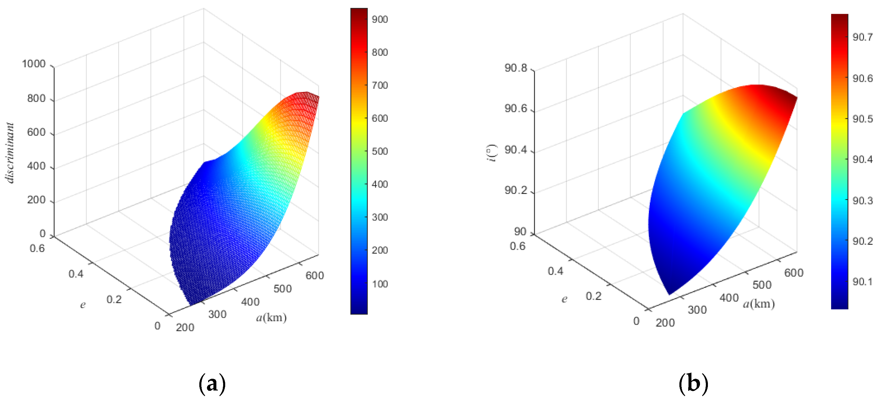
Figure 1a shows the values of the discriminant for
a and
e. We see the value of the discriminant is always non-negative, so Equation (
5) has one real root when
a and
e are given.
Figure 1a indicates that there exists one Sun-synchronous orbit around Vesta at a certain
a and
e.
Figure 1b shows the variations of inclination,
i, for different values of
a and
e.
The spacecraft in Sun-synchronous orbits of Vesta would be perturbed by the Sun. In the latter part of this section, we continue to investigate circular Sun-synchronous-orbit perturbations. The derivative of inclination is formulated using the Lagrange equations, and the secular term of the derivative of inclination in a period caused by solar gravity is [
20]:
where
is the angle between the motion of Vesta around the Sun and the equator of Vesta. For circular Sun-synchronous orbits, Equation (
11) is presented as:
where
is the ecliptic longitude of motions of the Sun. The phrase,
, in Equation (
12) is related to the local time at the descending node, and the derivation of inclination is determined since the local time at the descending node is fixed.
Since Vesta has no atmosphere, the atmospheric drag effect is ignored. For Vesta, the rotation period is 5.3421 h, and a 1-degree drift of the right ascension of ascending node results in a 53.421 s drift of local time at the descending node. Then, the drift of local time at the descending node caused by solar gravitation is:
where
and
are initial launch biases of
a and
i, respectively. Local time drift at the descending node comes from four variables in Equation (
13):
,
,
, and
. Let
be 0, and consider the remaining three items according to the following analysis. According to Equations (A.4) and (A.5),
is
for Vesta; this is about four orders of magnitude lower than
. Hence,
can be ignored.
Given an initial orbital element of circular Sun-synchronous orbits:
a = 508.27 km,
e = 0.0001,
i = 90.2990 deg,
deg,
deg, and
M = 0 deg, and the ecliptic longitude of the Sun is fixed at
deg. We chose a small initial orbital deviation to investigate the local time drift at the descending node during a 2-Earth-year period. For an initial orbital deviation of
km,
deg, and
deg,
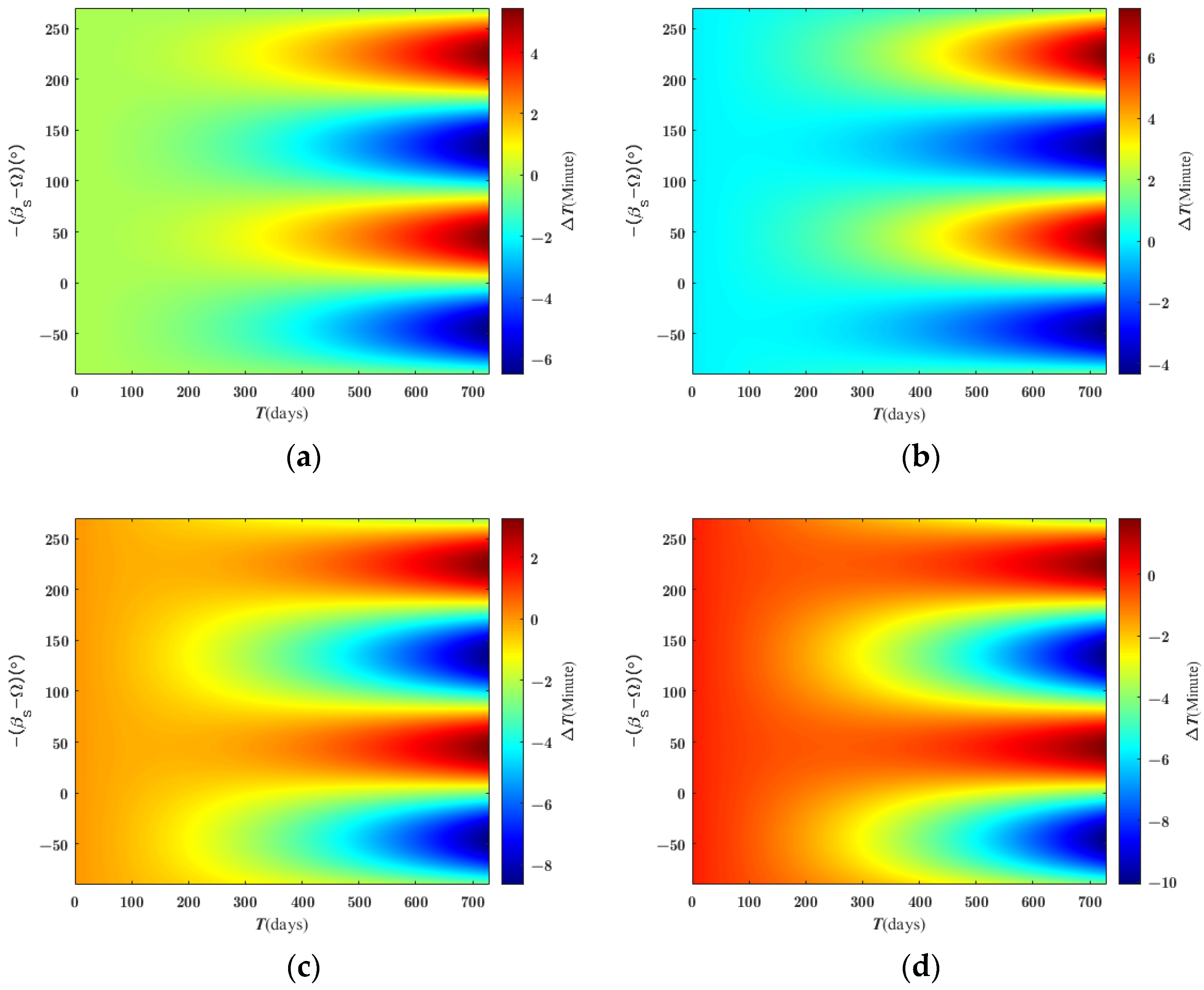
Figure 2a shows that the local time drift,
, is positive for
deg, which means the local time at the descending node will be delayed. In contrast, the local time at the descending node will be brought forward for
deg. Therefore, we set
at −45 deg, where the local time drift will obtain the extremum value at the end of 2 Earth years.
There are two kinds of methods to fix the local time at the descending node. One is the preset inclination bias method, and the other is the multiple inclination bias method [
34]. In the case of a preset bias, an initial inclination will be set in place of any other inclination controls during the spacecraft’s lifetime. This is simple and efficient for short-period missions, and the spacecraft will maintain the character of the Sun-synchronous orbits.
When
, the local time drift in Equation (13) obtains the extremum:
The local time drift at the descending node should be less than the extremum value during the spacecraft’s mission period:
, where
is the end time of the spacecraft’s mission period. Here, we set:
where
. Then we obtain
from Equation (13) for the following equation:
Let
. Then, based on Equations (15) and (16), the preset inclination bias is:
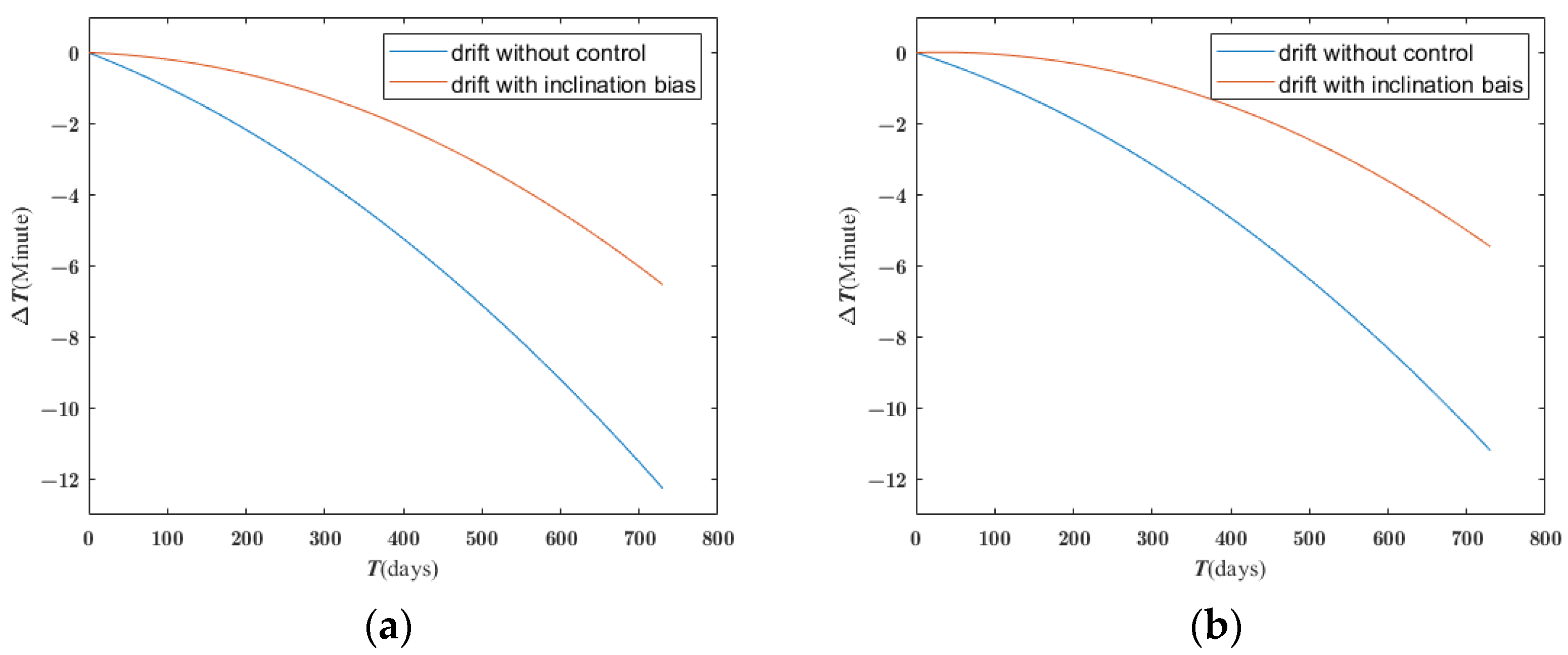
Figure 3 shows that the preset inclination bias method limits the local time drift at the descending node in a 2-Earth-year mission period.
The multiple inclination bias method utilizes a periodic inclination bias to reduce the local time drift caused by solar gravitation. In a period of
, the extremum of local time drift is equal to a fixed local time drift-bound
:
Due to the negligible
, using calculation in Equation (
13), Equation (
18) can be formulated as:
where
. When
, the following was obtained:
Then, the multiple inclination bias is as follows:
where
has a sign opposite to the sign of
. The multiple inclination bias is periodic during a long-period mission.
Figure 4 shows the multiple inclination bias method when the limited local time drift bound is 0.2 min. We can see that this method is sensitive to the initial inclination deviation. From
Figure 3 and
Figure 4, we can see that it is very important to limiting the initial inclination deviation.
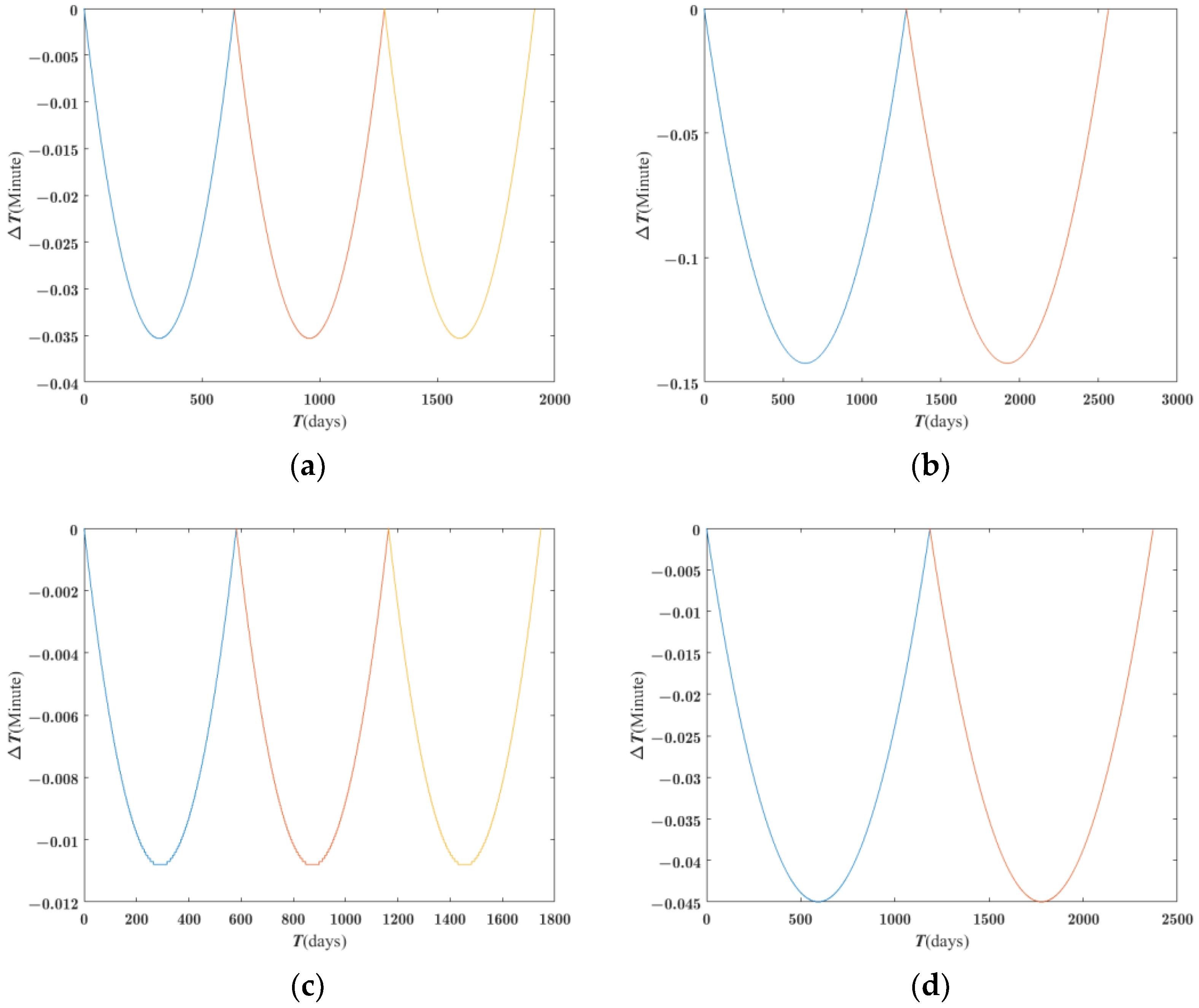
We applied the method in this section to the existence and control of Sun-synchronous orbits of Lutetia and Eros. Given the initial orbital elements of the circular Sun-synchronous orbit of Lutetia,
a = 186.49 km,
e = 0.00001,
i = 172.52 deg,
deg,
deg, and
M = 0 deg; and for the initial orbital elements of the Sun-synchronous orbit of Eros,
a = 118.72 km,
e = 0.60566,
i = 165.100 deg,
deg,
deg, and
M = 0 deg. Using the multiple inclination bias method,
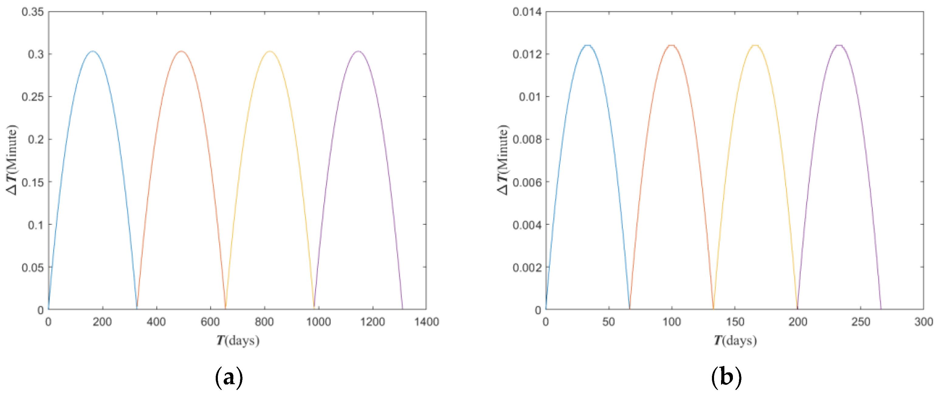
Figure 5 shows the local time drift change of the Sun-synchronous orbits of Lutetia and Eros, respectively. The local time drifts of the two orbits are not sensitive to the initial inclination deviation but are sensitive to the initial semi-major axis deviation. Compared with the Sun-synchronous orbits’ control period of Vesta, the control periods of the Sun-synchronous orbits of Lutetia and Eros are much longer.
3. Orbits with a Critical Inclination
The orbit with a critical inclination is described as critical as there is zero apogee drift for spacecraft in elliptical orbits at this inclination. This orbit is a practical option for long-term spacecraft flying around oblate planets such as Earth and Mars [
16]. The secular perturbations of the first and second order are considered in the investigation of orbits at the critical inclination of Vesta. The mean variation of eccentricity from the secular part of the first and second order are
To meet the condition for orbit with critical inclination, the average variation of the argument of perigee in the second equation of (A.6) needs to be zero; then, we obtain a quadratic equation of variable
where
Equation (
23) has two different real roots of
if the discriminate of
is non-negative.
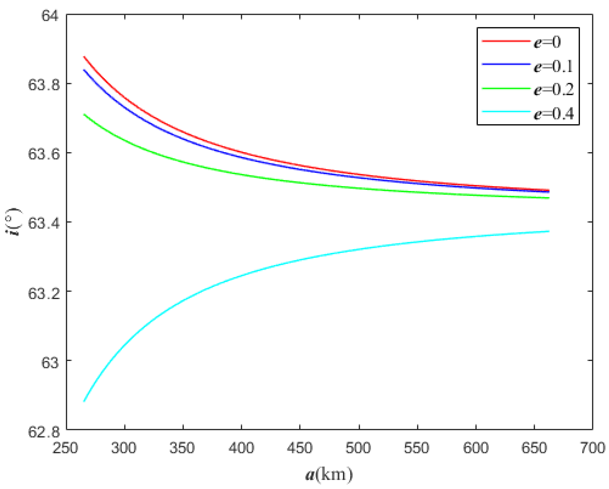
In
Figure 6, the variation of critical inclinations as the semi-major axis
a increases from 265 km to 663 km are presented. We note that the critical inclination decreases slowly and monotonically concerning the orbit’s altitude for
. For
, the critical inclination increases rapidly and monotonically. For Earth, the critical inclinations are fixed when considering only
J2, while in the case of Vesta, critical inclinations depend on the semi-major axis and eccentricity.
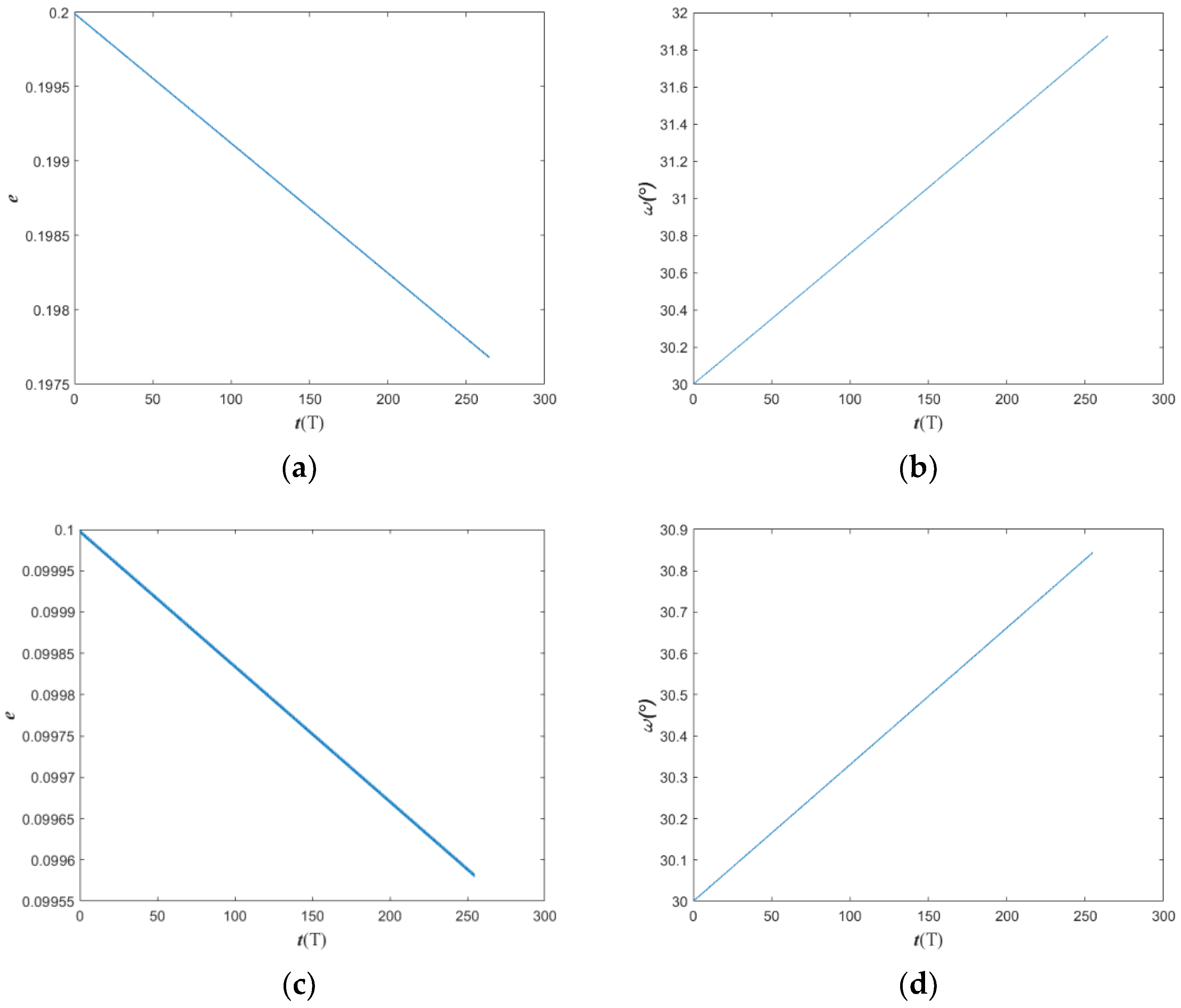
We chose two different orbits of critical inclination with
a = 492.171 km,
e = 0.2,
i = 63.499 deg, and
a = 522.580 km,
e = 0.1,
i = 63.519 deg, to evaluate the evolution of
and
e over a period of 250
T, where
T is a Vesta day. The zonal harmonic coefficients up to
J6 are considered, and the results are shown in
Figure 7. The drift amplitude of
is about 2 deg for 250
T, and the
e is about 0.0023 for the first case in
Figure 7. The drift amplitude of
and
e are slightly smaller in the second case since the altitude of the second orbit is higher near the stationary orbit of Vesta.
Some special properties were found when we applied the method in this section to Lutetia and Eros. For Lutetia, orbits with critical inclination do not exist with the condition of e < 0.6 and a > 153 km. For Eros, orbits with critical inclination do not exist with e < 0.9 and a > 91 km.
4. Repeating Ground-Track Orbits
Repeating ground-track orbits, which have regular ground-track patterns, are defined as orbits with the trajectory ground track repeating after a whole number of revolutions within some days. Repeating ground-track orbits represent an essential role in planet observation. We can monitor the area of Vesta by using spacecraft on these orbits and detect the surface and body of Vesta during a period. The interval of the adjacent ground track in the equator is
where
is the rotational angular velocity of Vesta, and
TN is the nodal period of the motion of the spacecraft, which is presented in Equation (A.11). The condition for achieving a repeating ground track can be written as
where
P and
Q are positive integers. Equation (
28) means spacecraft will have completed
P revolutions in
Q days of Vesta. With the definition of
in Equation (
27), Equation (
28) can be formulated as
where
Z =
P/
Q is the ground-track repetition parameter, widely used in practice.
and
are formulated in Equation (A.6). We can see that once the ground-track repetition parameter is given, Equation (
29) represents the relation between
a,
e, and
i. The repeating ground-track orbits are often Sun-synchronous, in which Equation (
4) is also satisfied. If
P and
Q are fixed, then
a and
i can be calculated. Based on Equation (
4), we can write Equation (
29) as
for a given ground-track repetition parameter, with Equations (A.1) and (A.6), Equation (
30) can be further formulated as a quadratic equation of variable
where
Equation (
31) has four real roots of variable
only if the discriminant of
is above zero.
The rotational angular velocity of Vesta is greater than the mean motion of Vesta around the Sun. Equation (
35) indicates that the lower bound of
Z is
Vesta rotates on its axis once every 5 h 20 m 30 s, which is denoted as
; the orbit period of spacecraft around Vesta
is 2 h 20 m 48 s at a low altitude of 50 km. The upper bound of
Z can be calculated by
, which is equal to 2.276. Concerning the semi-major axis for different
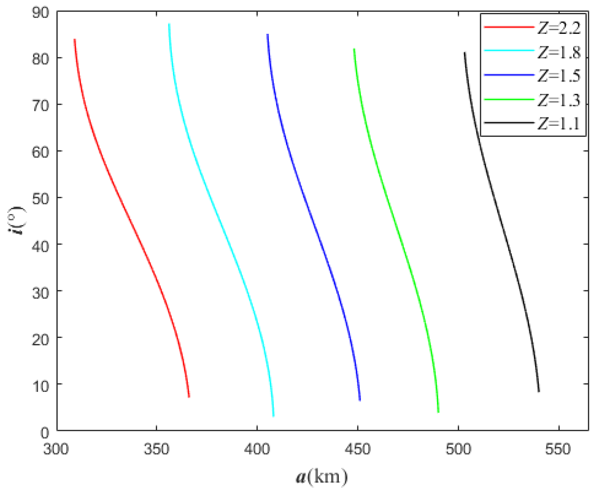
Z, the change of inclinations of Sun-synchronous repeating ground-track orbits is presented in
Figure 8. We can see that for a fixed
Z, the inclination decreases with respect to the semi-major axis monotonously, and it is sensitive to the change of the semi-major axis. For
Z = 1.1, the maximum meaningful semi-major axis is 540 km near the stationary orbit of Vesta. Compared with major planets in the solar system, such as Earth, Mars, Jupiter, and Saturn, Vesta’s ground-track repetition parameter is small [
16,
19,
35]. For Mars, the repetition parameter is roughly between 12 and 14 [
16]. For Jupiter, it is roughly between 2.5 and 3.5 [
19]. Larger repetition parameters can offer a larger scale selection for Sun-synchronous repeating ground-track orbits.
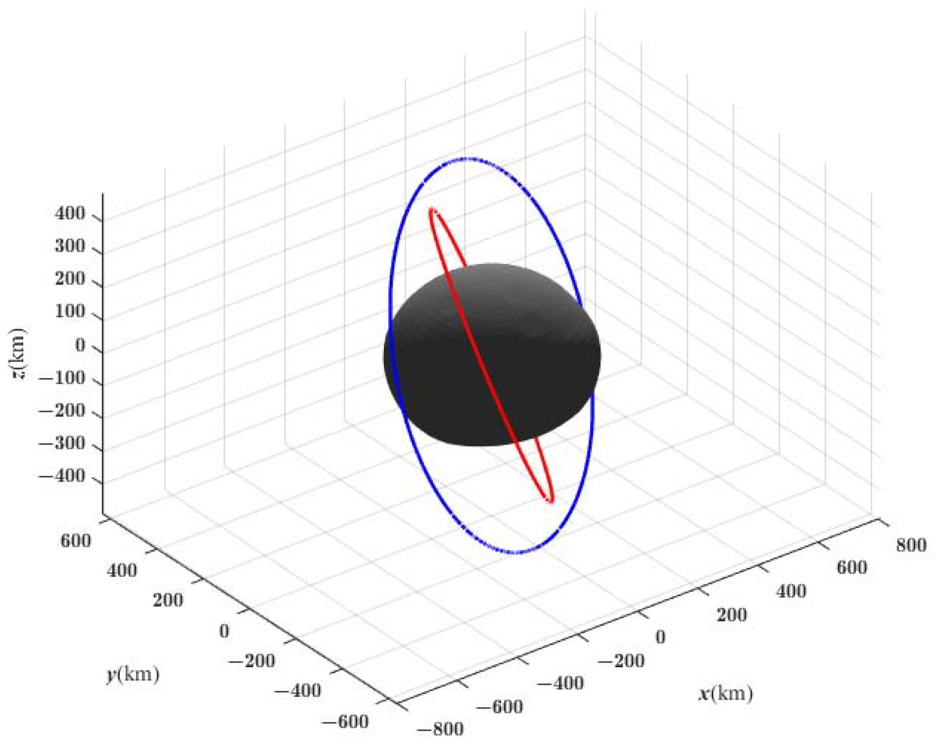
Figure 9 shows Vesta’s Sun-synchronous repeating ground-track orbit for a given repetition parameter.
We also calculated the discriminant in Equation (
35) for Lutetia and Eros. We found that Equation (
31) has no real root for Lutetia and Eros in the case of
e = 0, which means that there are no Sun-synchronous repeating ground-track circular orbits for Lutetia and Eros. On the other hand, for the case of
e > 0, there are a few Sun-synchronous repeating ground-track orbits for Lutetia and Eros when
e > 0.9.
5. Stationary Orbits
A stationary orbit, also called a synchronous equatorial orbit, is a type of synchronous orbit around a planet or moon where the orbit is directly over the equator. We call it a synchronous orbit (SO) for Vesta, known as geosynchronous equatorial orbit (GEO) for Earth. Spacecraft in the stationary orbit remain orbiting over the same spot on the planet’s surface and would appear to be standing still above the surface. The most preferred use for spacecraft in this orbit is for communication, navigation, and space science. The spacecraft in the stationary orbit must satisfy very precise conditions to a fixed position related to the orbiting planet, and its orbit positions are given in the form of a station longitude. We will investigate the existence of the stationary orbits of Vesta in this subsection.
Based on Equations (A.12) and (A.13), spacecraft in the stationary orbits of Vesta must satisfy the following condition [
19]
When we set
and
, the first Equation of (A.13) can be written as
Solving Equation (
38) with the condition in Equation (
37), we obtain the radius of the stationary orbit of Vesta, which is 549.74 km.
We continue to analyze the perturbation of the SO and slightly inclined synchronous orbit (ISO) caused by solar radiation pressure, leading to drift of eccentricity. The solar radiation pressure on spacecraft in SO or slightly ISO is
where
K is the reflection parameter of the spacecraft,
p is the intensity of solar radiation pressure,
A is the area of the spacecraft vertical to the Sun,
m is the spacecraft’s mass, and
S is the unit vector from the spacecraft to the Sun. We use
S in this section as an approximation of the vector from Vesta to the Sun.
S can be expressed as
where
is the angle between solar radiation direction and
X axis and
is the obliquity of the ecliptic plane of Vesta,
. The average distance from Vesta to the Sun is 353.4 million km, and the mean solar irradiance around Vesta is 247.41 W/m
2 [
36]. Then, we obtained the solar radiation pressure of
for a spacecraft with the following parameters: reflection parameter
K = 1, average area
A = 10 m
2, and mass
m = 1000 kg.
In the Radial–Tangential–Normal coordinate system, the components of
are:
where
is the unit vector in the kinetic coordinate system [
34]. The average derivatives of the eccentricity vector
,
are as follows:
We further formulated Equation (
42) as [
34]:
When considering the solar radiation pressure perturbation over a long period of time, we obtained the following expressions of the eccentricity vector:
Then, the eccentricity vector can be further formulated as:
We observed from Equation (
45) that the curve of the eccentricity vector is an ellipse caused by the solar radiation pressure. The eccentricity vector moves along the curve of the ellipse during Vesta’s orbit around the Sun. The semi-major axis of the ellipse is
, and the semi-minor axis of the ellipse is
.
We then analyzed the inclination change caused by solar radiation pressure. Based on Equation (
41) [
34], we can write the normal perturbation force caused by solar radiation pressure as:
where
. The derivatives of the inclination vector are:
For a spacecraft in SO or slightly ISO,
,
.
should be constant during one Vesta rotation period; thus, the time integral of the inclination vector in a Vesta rotation period for time
t is:
We learn from Equation (
49) that the curve of the inclination vector is a circle caused by the solar radiation pressure; the inclination vector moves on the circle with the period of one Vesta day, and the circle’s radius is less than
deg.
After analyzing the eccentricity drift and inclination drift caused by solar radiation pressure perturbation, we calculate the eccentricity drift and inclination drift caused by solar gravitation perturbation. The average time derivatives of the eccentricity vector
are:
where
is the angle between two unit vectors; one is the unit vector from the center of Vesta to the Sun, and the other is the unit vector from the center of Vesta to the spacecraft in SO,
. Due to the existence of the trigonometric function of
l in the first equation of (50), the drift of
caused by solar gravitation is periodic. In the case of the second equation of (50), there is no secular term in the right hand of the equation, so the drift of
caused by solar gravitation is also periodic.
Before analyzing the inclination drift caused by solar gravitation perturbation, we obtained the normal perturbation force caused by solar gravitation, which can be written as [
37]:
The derivatives of the inclination vector perturbed by the solar gravitation are:
The short periodic terms in Equation (
52) were neglected for a long period, and the derivatives of the inclination vector were further formulated as:
For a spacecraft in SO or slightly ISO,
,
. The time integral of the inclination vector in a period of Vesta orbiting around the Sun for time
t is:
We learned from Equation (
54) that the drift of
caused by solar gravitation is periodic, with a period of half of a Vesta year. If only the secular term of
is considered, the drift of inclination throughout
T is:
We obtained
deg over one Vesta year from Equation (
55). For Earth, we learned that
is 0.2712 deg over one Earth-year period.
6. Conclusions
We analyzed the existence of some types of orbits around Vesta, including the Sun-synchronous orbits, orbits with critical inclination, repeating ground-track orbits, and stationary orbits. Zonal harmonic coefficients J2, J3, and J4 were considered in the gravitation model of these typical orbits. For the evolutionary evaluation of an orbit with a critical inclination, coefficients up to J6 were considered.
First, we investigated the existence of Sun-synchronous orbits of Vesta, found the variations of inclination for different semi-major axes and eccentricity values, and calculated the local time drift at the descending node caused by solar gravitation. Then, two control methods were given to dampen the local time drift and applied to Lutetia and Eros. As a result, the control periods of Sun-synchronous orbits of Lutetia and Eros were found to be much longer.
Second, we analyzed the orbits with critical inclinations. In the case of Vesta, critical inclinations depend on the semi-major axis and eccentricity. When the zonal harmonic coefficients up to J6 were considered, the eccentricity and the argument of perigee changed monotonically. Numerical calculation results showed that orbits with critical inclinations at a high altitude do not exist for Lutetia and Eros.
Third, we calculated different repetition parameters of repeating ground-track orbits of Vesta. Compared with major planets in the solar system, Vesta’s ground-track repetition parameters are small. We found that Sun-synchronous repeating ground-track circular orbits do not exist for Lutetia and Eros.
Finally, we calculated the radius of stationary orbits of Vesta in the spherical coordinates of an inertial frame. Then, we analyze the inclination and eccentricity drift caused by solar radiation pressure and solar gravitation, respectively. We found that, in the case of solar radiation pressure perturbation, the eccentricity vector moves on an ellipsis and the inclination vector moves on a circle. For the case of solar gravitation, the drift of the eccentricity vector is periodic, and the drift of inclination in the direction of the X axis is 0.0119 deg over a Vesta year.


