Article

Transient Thrust Analysis of Rigid Rotors in Forward Flight

1
Aerospace Engineering, Ryerson University, 350 Victoria St., Toronto, ON M5B 2K3, Canada
2
Applied Research Laboratory, The Pennsylvania State University, 229 Hammond Bldg, University Park, PA 16802, USA
*
Author to whom correspondence should be addressed.
Aerospace 2022, 9(1), 28; https://doi.org/10.3390/aerospace9010028
Submission received: 6 December 2021 / Revised: 27 December 2021 / Accepted: 28 December 2021 / Published: 5 January 2022
(This article belongs to the Special Issue Helicopter Aerodynamics)

Abstract

:
The purpose of this study was to investigate and quantify the transient thrust response of two small rigid rotors in forward flight. This was accomplished using a distributed doublet-based potential flow method, which was validated against wind-tunnel experimentation and a transient CFD analysis. The investigation showed that for both rotors, advancing and retreating blade effects were predicted to contribute to transient thrust amplitudes of 5–30% of the mean rotor thrust. The thrust output amplitudes of individual rotors blades were observed to be 15–45% of the mean rotor thrust, indicating that it is not uncommon for the thrust output variation of an individual rotor blade to approach the same value as the mean thrust output of the rotor itself. In addition to this, the theoretical analysis also illustrated that higher blade thrust oscillations resulted in pronounced asymmetric rotor wake structures.

1. Introduction

The thrust acting on a rotor in forward flight may vary with time due to advancing and retreating blade effects acting on the individual rotor blades. While conventional helicopters compensate for these effects with hinged blades, small multirotor vehicles typically use rigid rotors. Without compensation, the thrust output of the rotor is transient, with the amplitude being linked to the forward speed and angle of the vehicle, as well as the rotational velocity of the rotor. Transient thrust has potential implications for both the control systems and the structural design of the rotor blades and central chassis due to fatigue. Despite these potential implications, quantification of the time-dependent thrust on rigid rotors at various tip-plane angles of attack is notably lacking in the literature. The purpose of this study is to investigate and quantify the transient thrust response of small rigid rotors in forward flight under various operating conditions through numerical predictions of unsteady blade and wake effects.
Historically, research into small propellers or rotors has focused on steady-state conditions or time-averaged forces. There has been a substantial amount of research in documenting the performance of small propellers in steady axial flow. One such example is the University of Illinois at Urbana-Champaign (UIUC) Propeller Database created through the work of Brandt, Deters, Ananda, and Selig ([1,2]). A few studies have experimentally investigated the time-averaged forces of rigid rotors in forward flight, as are experienced by the rotors of a multirotor vehicle. Experimental data sets of this nature are available through Kolaei et al. [3] and Serrano et al. [4].
In one notable recent study, Misiorowski et al. [5] quantified the transient thrust oscillations of a single isolated rigid rotor at a one operating condition. This analysis was conducted using a Navier–Stokes solver and was done in the course of quantifying rotor interactions on quadrotors. In addition to providing sectional thrust coefficient values as a function of azimuth location, the authors also provided insights on the asymmetric nature of the wake rollup downstream due to advancing and retreating blade effects. These findings highlight a need for more in-depth analysis of small, rigid rotors operating in unsteady conditions.
There are several approaches described in the literature for the prediction of rotor performance in forward flight, which can be grouped according to the assumptions applied in each. Methods based on blade element momentum theory are presented by Carrol [6] and Serrano et al. [4]. Both of these methods show good agreement with time-averaged experimental data, but use simplified inflow models that are based on momentum theory and are therefore not suited to investigating transient thrust loads under highly unsteady conditions.
Potential flow-based methods are frequently used in modeling unsteady systems, including rotors in forward flight. One of the most common potential flow methods for this nature of analysis is the unsteady vortex lattice method (UVLM), outlined by Katz and Plotkin [7]. This method uses constant-strength vortex rings to model lifting surfaces and wakes. Further information, including examples of unsteady applications, are provided by [8,9,10]. The unsteady vortex lattice method has also been extended and improved upon in various ways, including by using vortex particle wake models [11,12,13] and modeling leading-edge vortex shedding [14].
Other potential flow methods such as RCAS [15] and CAMRAD [16] are commonly used in helicopter design and analysis. These methods use lifting line theory for their aerodynamic approximations and can be used with fixed or free vortex wakes. Due to a lack of performance prediction tools directed at small rigid rotors, Russell and Sekula [17] evaluated CAMRAD II for modeling the time-averaged thrust and power of a rigid rotor in hover, ultimately determining that it is well-suited for this application through comparisons to experimentally-obtained data. Leishman et al. [18] summarized free-vortex methods and filament-based potential flow methods for helicopter rotor analysis. These methods were born out of the need for higher fidelity wake modeling. Leishman provides a case for the importance of relaxed wake modeling in rotor analysis, asserting that interactions between the wake vortices and the rotor cannot be easily generalized and the use of a relaxed wake model is beneficial. Free-vortex methods typically model the wake as a single trailing tip vortex of constant strength to reduce computational expense. Further details on this wake model, as well as potential improvements, are given by Govindarajan and Leishman [19].
Barcelos et al. [20] used a quasi-steady potential flow-based method first introduced by Bramesfeld and Maughmer [21] to analyze quadrotor flight configurations. This method eliminates the trailing vortices present in conventional vortex lattice methods by replacing them with vortex sheets. As the analysis was quasi-steady, streamwise changes in shed circulation were not modeled in the wake, and impulse forces were not approximated.
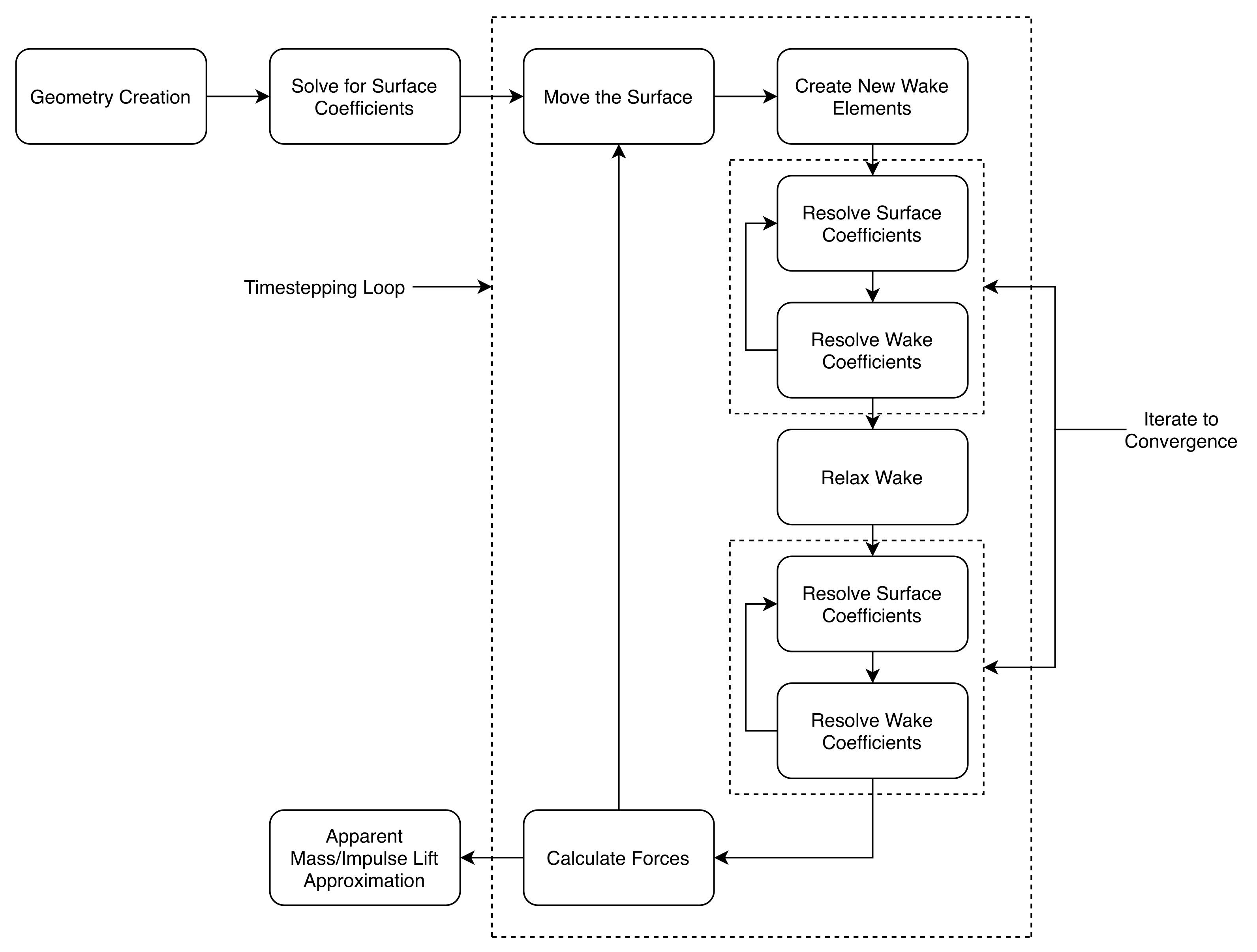
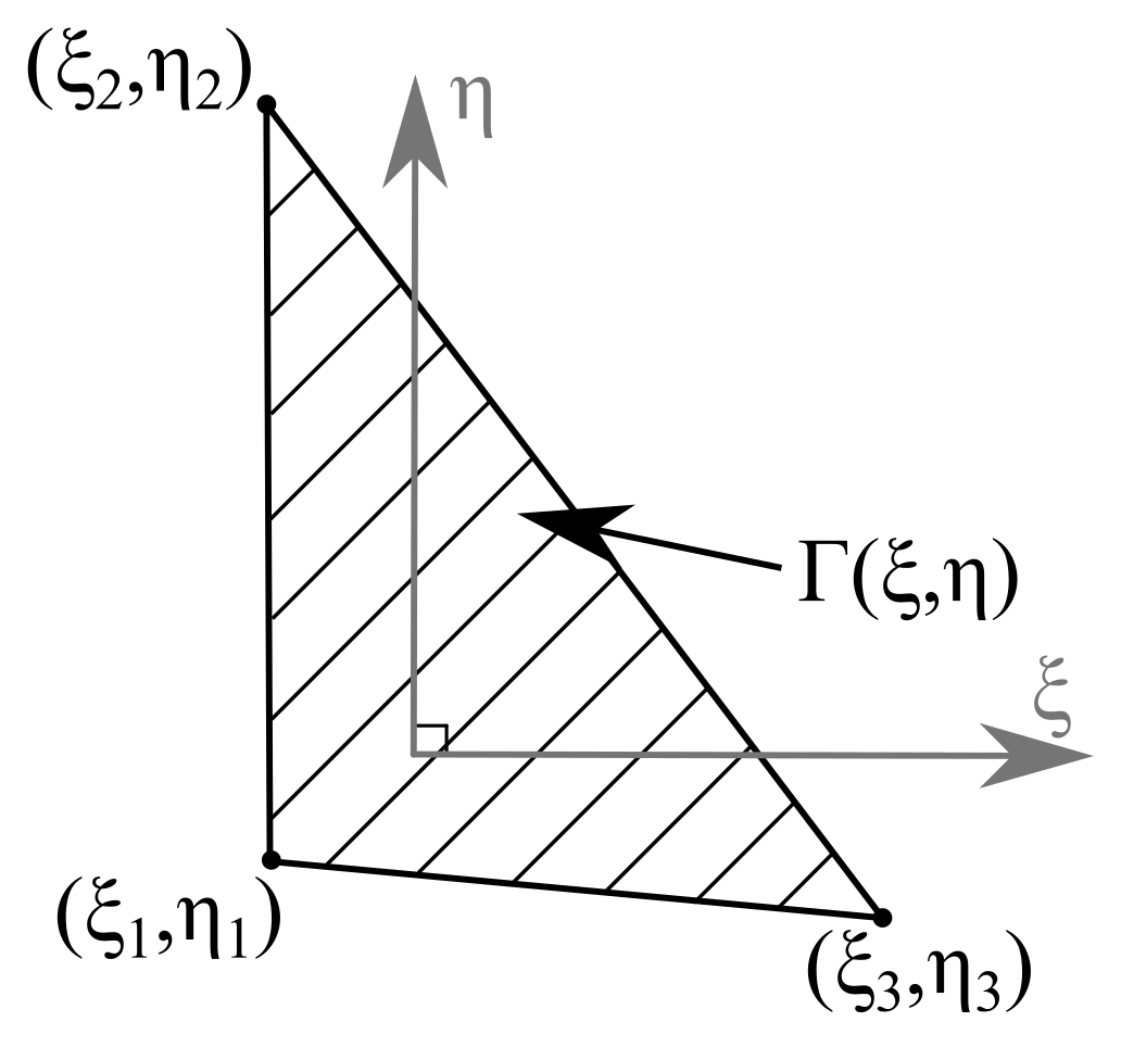
A new potential flow method is used in this study to predict unsteady rotor thrust. This method is referred to as the DDE method because it uses distributed doublet elements (DDEs) to model unsteady systems with complex wake interactions. The lifting surfaces and wakes are discretized and represented as a network of planar distributed doublet sheets with continuous higher-order strength distributions, resulting in a velocity field that is defined everywhere. This reduces the number of singularities in the system when compared to vortex filament-based methods, such as UVLMs, and leads to a robust unsteady relaxed wake model. In addition to this, the distributed nature of the element strength alleviates timestep-size constraints which exist for some UVLMs.
In this study, both experimentally-obtained data, as well as transient blade loads predicted by Misiorowski et al. [5], are used to validate the DDE method for unsteady rotor analysis in forward flight. The DDE method is then used in turn to provide a detailed analysis of the transient thrust response of two different rotors in partial and fully edgewise flow. This approach was chosen because even though experimental testing is one approach to understanding how rotor thrust oscillates over time in edgewise or near-edgewise flow, most rotor-test stands are unable to distinguish the individual thrust contributions from each blade. Likewise, using flow visualization is infeasible for small-scale rotors at comparatively high rotational speeds. Through using computational modeling, such as the DDE method, it is possible to break down the rotor response into the response of the individual blades and their interactions with the rotor wakes and freestream.

2. Materials and Methods

2.1. Experimental Testing

In this study, experimental data is used to validate the time-averaged thrust predictions of the DDE method. This is done as a method of verifying the thrust predictions of the DDE method before it is applied to evaluating transient thrust loads. In wind-tunnel tests, these time-averaged rotor-thrust loads were determined for a number of different forward speeds and angles of attack. The data was obtained using Ryerson University’s (RU) subsonic wind-tunnel and its rotor-test stand.

2.1.1. Description of Experimental Setup and Conventions

A sketch of the wind-tunnel is shown in Figure 1. It is a closed-return tunnel with a test section of length 1.5 m and cross-sectional size of 0.914 m × 0.914 m. For the purposes of this study, airspeeds ranging from 5–25 m/s were reached in the test section, corresponding to turbulence intensities of approximately 0.2–0.3% as reported by Kolaei et al. [3]. This reference also lists further details on the wind-tunnel, experimental test procedures, and data corrections.
The rotor-test stand that was used for this study is based on the ATI Mini45 six-degree-of-freedom load cell, with a resolution of 1 / 16 N in the thrust direction [22]. As shown in Figure 2a, the stand was mounted on a turntable, thus enabling tip-path plane angles of attack ranging from 90 to 90 . The definition of the tip-path plane angle of attack is shown in Figure 2b. For example, a tip-path plane angle of attack of 0 represents inflow parallel to the rotor plane.
This study distinguishes between propeller and rotor conventions for advance ratio and thrust coefficient. Propeller convention is used only in this section, in comparison with data from the UIUC database. The propeller advance ratio (J) is defined as:
J = V n D
where V is the freestream velocity, n is the rotational speed in revolutions per second, and D is the propeller diameter. The propeller thrust coefficient ( C T p ) is defined as:
C T p = T ρ n 2 D 4
where T is the thrust force and ρ is the air density.
The results presented in later sections of this study are given in terms of normalized freestream velocity, rotor thrust coefficient, and the aforementioned tip-path plane angle of attack. For the purposes of this study, normalized freestream velocity is defined as the ratio of a rotor’s inflow velocity magnitude to its rotational speed:
μ = V Ω R
where R is the rotor radius and Ω is the rotational speed in radians per second. The rotor thrust coefficient is:
C T = T ρ A ( Ω R ) 2
where A is the rotor disk area.

2.1.2. Verification of the Rotor-Test Stand

In order to substantiate the experimental results from the rotor-test stand, a Master Airscrew (MA) 11x7E propeller was evaluated at various propeller advance ratios. These results were compared with published data from the UIUC Propeller Database ([1,2]), which also lists the geometry of the propeller. Thrust and power coefficients at various advance ratios are compared in Figure 3. Maximum deviations between the RU and UIUC experimental results are less than 3 % , up to an advance ratio of approximately 0.5 for both thrust and power coefficients, with these deviations growing with increasing advance ratio as the propeller approaches a windmilling state.

2.1.3. T-MOTOR 18x6.1 Rotor Testing

A T-MOTOR 18x6.1 carbon fiber rotor was evaluated at angles of attack of 0 , 15 , and 90 at various normalized freestream velocities with a fixed rotational speed of 3000 RPM. The geometry of the T-MOTOR 18x6.1 was obtained from a three-dimensional scan presented by Kolaei et al. [3], who provide the chord and twist distributions, shown in Figure 4, as well as section data.

2.2. Computational Modeling

When using the DDE method, the entire rotor and wake are modeled using distributed doublet sheets. The strength of the doublet distribution is second-order in both the spanwise and streamwise directions, resulting in a system which is equivalent to that of an infinite number of vortex rings of varying strengths. As such, this model is more computationally expensive than free-vortex methods, though the second-order strength distribution results in fewer elements required to model spanwise or streamwise changes in circulation when compared to a first-order method. The primary benefit of the DDE method is that there are no vortex filaments or sources of lumped vorticity anywhere in the system. With a continuous distribution of doublet strength between elements, there is no need for corrective actions to manage singularities, such as the solid-core models or cut-off distances used with vortex filaments. This allows for a truly unsteady relaxed wake model, with both spanwise and streamwise changes in strength, without the wake diverging due to large induced velocities from vortex filaments.

2.2.1. Overview of the Method

What follows is a brief summary of the DDE-based method, with greater detail provided by Krebs [23]. An overview of the method is shown in Figure 5. To begin, the surface geometry is discretized into planar triangular elements. The initial strengths of these elements are determined by imposing flow tangency conditions at all element control points, as well as a necessity for the strength to be continuous across all elements. A timestepping procedure then commences and a new row of triangular wake elements is created. The strengths of these new wake elements are assigned during the timestep in which they are created and then held constant for all future timesteps. The wake is then relaxed, and the strength coefficients are updated to account for the stretching of the wake elements. Forces are calculated using the Kutta–Joukowski theorem at the trailing edge of the lifting surface, for both freestream and induced forces.
The doublet strength across an element, analogous to circulation for this application, is defined as:
Γ ( ξ , η ) = 1 2 A 1 η 2 + A 2 η + 1 2 B 1 ξ 2 + B 2 ξ + C 2 η ξ + C 3
with A n , B n and C n representing the coefficients of the circulation distribution and ( ξ , η ) representing the local element coordinate system as depicted in Figure 6.
As outlined by Drela [24], the velocity field induced by a distributed-doublet element with strength Γ ( ξ , η ) is given by:
V = Γ ( ξ , η ) n ^ | r s | 3 3 n ^ · ( r s ) r s | r s | 5 d η d ξ
with the normal vector represented by n ^ , the location of the field point represented by r, and the location of the differential element on the surface of the DDE given by s. The influence coefficients for DDEs are obtained by solving Equation (6) in terms of the six coefficients of the circulation distribution. This is accomplished through the method outlined by Johnson [25] for the evaluation of doublet integrals for an arbitrary field point.
At the leading edge and tips of lifting surfaces, the doublet strength is prescribed as zero. At the trailing edge of lifting surfaces, the doublet strength is carried into the wake. Surfaces and wakes are modeled with zero thickness, with surface elements being placed along the camber line of the wing, rotor, or propeller. Using a zero-thickness model avoids any issues that could arise from wake piercing, where wake elements enter into the interior of a body as can be observed with panel codes and strong aerodynamic interactions [26]. Additionally, the rotors used on multicopters are typically thin, with the T-MOTOR 18x6.1 from this study having a maximum thickness of approximately 5% of the chord.
As shown in Figure 5, the DDE method uses two iterations within each timestep to achieve equilibrium between the surface element and newly-created wake element strengths, with one being performed before and one after the wake relaxation procedure. As the strength of the surface elements impacts the strength of the newly-created wake elements, and as the newly-created wake elements impact flow-tangency through their induced velocities, the strengths of the surface and wake elements are intertwined. These iterations are necessary in order to ensure that flow tangency and the Kutta condition are adhered to within each timestep, especially in unsteady analyses. A single iteration of this process is often not enough to reach equilibrium, leading to a lack of flow tangency and a solution that is dependent on the timestep size. This iteration-based technique is described by Katz and Plotkin [7] when discussing unsteady motion of a two-dimensional thin airfoil. Murua [27] mentions the possibility of implementing such a scheme within the UVLM, though they do not due to the computational expense.

2.2.2. Unsteady Aerodynamic Predictions

The prediction of unsteady rotor loads can present challenges when using conventional vortex lattice methods. One such example is the ratio of timestep size to distance traveled by the surface elements. Simpson and Palacios [28] used an unsteady vortex lattice method (UVLM) outlined by Katz and Plotkin [7] and found that newly shed wake panels should be of approximately equal area compared to the trailing-edge surface elements from which they inherit their circulation strength. That is to say, the distance traveled by the surface elements each timestep, denoted by Δ x w , should be approximately equal to the chord length of the trailing edge surface element, denoted by Δ x c . The first reference to the constraint found in the literature was in the work of Rusak et al. [29], who note that vortex–lattice methods tend to be unstable when the wake element length is less than that of the surface element. A possible reason for this instability may be due to the finite-differencing methods that are typically used in UVLMs to determine the apparent mass or non-circulatory force. The apparent mass term is a necessary component of the unsteady Bernoulli equation. However, enforcing a timestep size constraint such as Δ x w / Δ x c 1 while analyzing rotors is problematic, since the distance traveled by the surface elements of rotors depends on their distance from the axis of rotation. Forward flight, with edgewise flight components, compounds this problem, as the distance traveled by surface elements then also depends on their azimuthal location.
Since its second-order distributed doublet sheets can be imagined as a system of infinitely small vortex rings, the timestepping portion DDE method inherently satisfies this constraint of Δ x w / Δ x c 1 . Modeling a DDE solution with a conventional vortex–lattice method would require an infinite number of elements, leading to both Δ x w and Δ x c being infinitesimally small, and therefore satisfying Δ x w / Δ x c 1 . Non-circulatory forces are accounted for via an approximation of the time rate of change of circulation for the unsteady Bernoulli equation, as outlined by Cole [30]. This is performed after the timestepping loop as shown in Figure 5, and can be done with a timestep size different than the one used within the timestepping loop to ensure that the constraint Δ x w / Δ x c 1 is maintained. This guarantees the stability of the apparent mass approximation, independent of the velocity or distance traveled by a surface element inside of a timestep. Unsteady analysis using the DDE method also involves maintaining individual wake element strengths over time, which ensure that streamwise changes in the shed circulation are possible. These characteristics enable the DDE method to represent fully unsteady flow regimes without discarding any effects as described by Drela [24].
To demonstrate the effectiveness of the DDE method for unsteady analysis, Figure 7 shows the response of a two-dimensional wing section to a sharp-edged gust for a number of different Δ x w / Δ x c ratios. These ratios were obtained by using different timestep sizes and chordal element counts, with the number of chordwise elements indicated by the parameter M. The analytical solution to this sharp-edged gust response is given by the Küssner function, as outlined by Leishman [31] and Kayran [32].
The results presented in Figure 7 indicate that there is an independence from the Δ x w / Δ x c ratio and timestep size for the DDE method. Though the ratios for each chordwise element count in Figure 7 vary by a factor of ten, there is very little difference in the lift coefficient across the gust response. The solution is relatively independent of timestep size as there are no discrete shed filaments, but rather a network of continuous distributed doublet sheets.
The solution does have a dependency on the number of chordwise elements, however. The results in Figure 7b indicate that an increase in the number of chordwise elements, M, results in a reduced error when compared to the analytical solution regardless of the time-step size or ratio. An increase in the chordwise resolution results in an increase in flow tangency conditions in the streamwise direction, meaning a sufficient resolution is necessary for good agreement with the Küssner function. As the chordwise strength across a single DDE is represented with a second order polynomial, as indicated by Equation (5), there is a limit to the complexity possible in the chordwise circulation when using a low chordwise element count. With a chordwise element count of M = 5 , the number used to model the rotors for this study, the percent deviation from the analytical solution reaches a maximum of approximately 15% before reducing sharply. In the case of this study, the rotor blades are not being subjected to a discontinuous velocity field across their span, but likely only in small localized areas. Due to these factors, the error represented in Figure 7b is deemed acceptable.

2.2.3. Rotor Performance Predictions

The DDE-based method was used to analyze the unsteady thrust of rotors. An example of such an analysis is shown in Figure 8, which depicts a top-down view of a rotor in fully-edgewise flow, meaning the inflow is parallel to the rotor plane. The rotor is moving from right to left while rotating counter-clockwise and each blade is shedding wake elements of their own color. Though the forces reported from the DDE-based method are relatively independent of timestep size, within reason, the example that is shown in Figure 8 uses 40 azimuth locations per revolution to ensure that the wake is represented at an adequate resolution for the relaxation procedure.

2.2.4. Validation of the DDE Method

Time-averaged thrust coefficients for the T-MOTOR 18x6.1 rotor, as predicted by the DDE method, are provided in Figure 9 for tip-path plane angles α t p p = 0 , 15 , and 90 . These are plotted alongside the experimental measurements obtained using the RU rotor-test stand, with the error bars defined according to the uncertainty analysis conducted by Kolaei et al. [3]. The percent deviation in thrust between the DDE method and the experimental data is less than 10 % for the forward flight cases at α t p p = 0 and 15 across the range of normalized freestream velocities. The largest percent deviation in reported thrust between the DDE method and the experimental data comes as the rotor approaches a windmilling state in fully axial flow at α t p p = 90 , where the thrust loads become relatively small. In general, the thrust loads predicted by the DDE method agree reasonably well with experimental results, even for highly unsteady cases of fully edgewise flight with significant surface-wake interaction.
The transient results of the DDE-based method were evaluated by comparing them to the single-rotor CFD simulation prediction presented by Misiorowski et al. [5], which uses a Navier–Stokes solver with a detached-eddy simulation model. An APC 12x5.5MR rotor was evaluated at a tip-path plane angle of attack of α t p p = 5 and a normalized freestream velocity of μ = 0.162 , in accordance with the geometry and operating conditions specified by Misiorowski et al. [5]. The results are shown in Figure 10, which displays the sectional thrust coefficient of a single blade of the rotor, d C T / d ( r / R ) , which was determined using Equation (4), and differentiating with the non-dimensionalized spans of the sections. When discussing azimuthal location in this study, the angles ψ = 0 and ψ = 180 correspond to the rotor blades being oriented parallel to the projection of the freestream vector onto the rotor plane, as shown in Figure 10. The blade beginning in the downstream-oriented position at ψ = 0 is advancing through azimuthal locations ψ = 0 180 and retreating through ψ = 180 360 . The opposite is true of the other blade.
Both the CFD and DDE method predictions show equivalent minimum and maximum sectional thrust coefficients of approximately 0 and 0.021, respectively. The maximum sectional thrust occurs at approximately 0.75 r / R in approximately the same azimuthal location of approximately ψ = 120 . Despite some minor differences on the retreating side where very low thrust coefficients are observed, the highly-unsteady DDE and CFD predictions agree quite well in magnitude.

3. Results

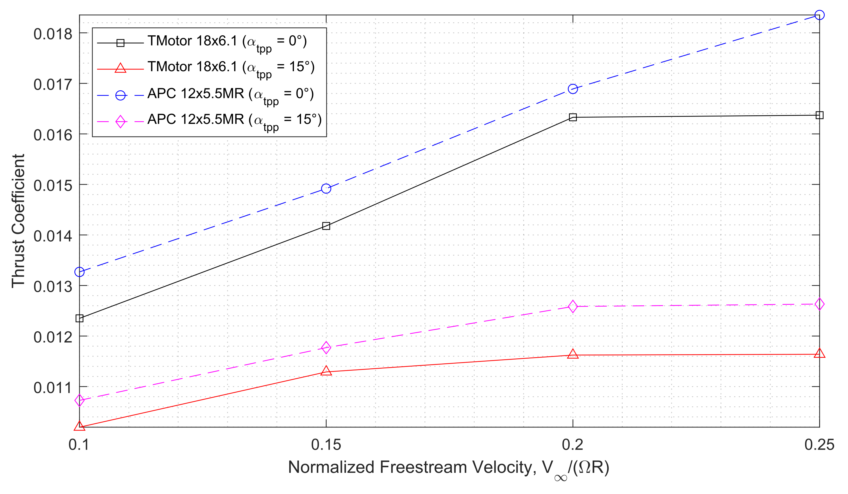
Using the DDE-based method, the T-MOTOR 18x6.1 and APC 12x5.5MR rotors were analyzed at various normalized freestream velocities at tip-path plane angles of α t p p = 0 and 15 , resulting in four unique datasets. An overview of the time-averaged thrust coefficients plotted against normalized freestream velocity is given in Figure 11. For both rotors, the rate of change of the thrust coefficient with normalized freestream velocity is higher at an angle of attack of α t p p = 0 . For both angles of attack, the APC rotor has a higher predicted thrust coefficient than the T-MOTOR across the range of normalized freestream velocities.
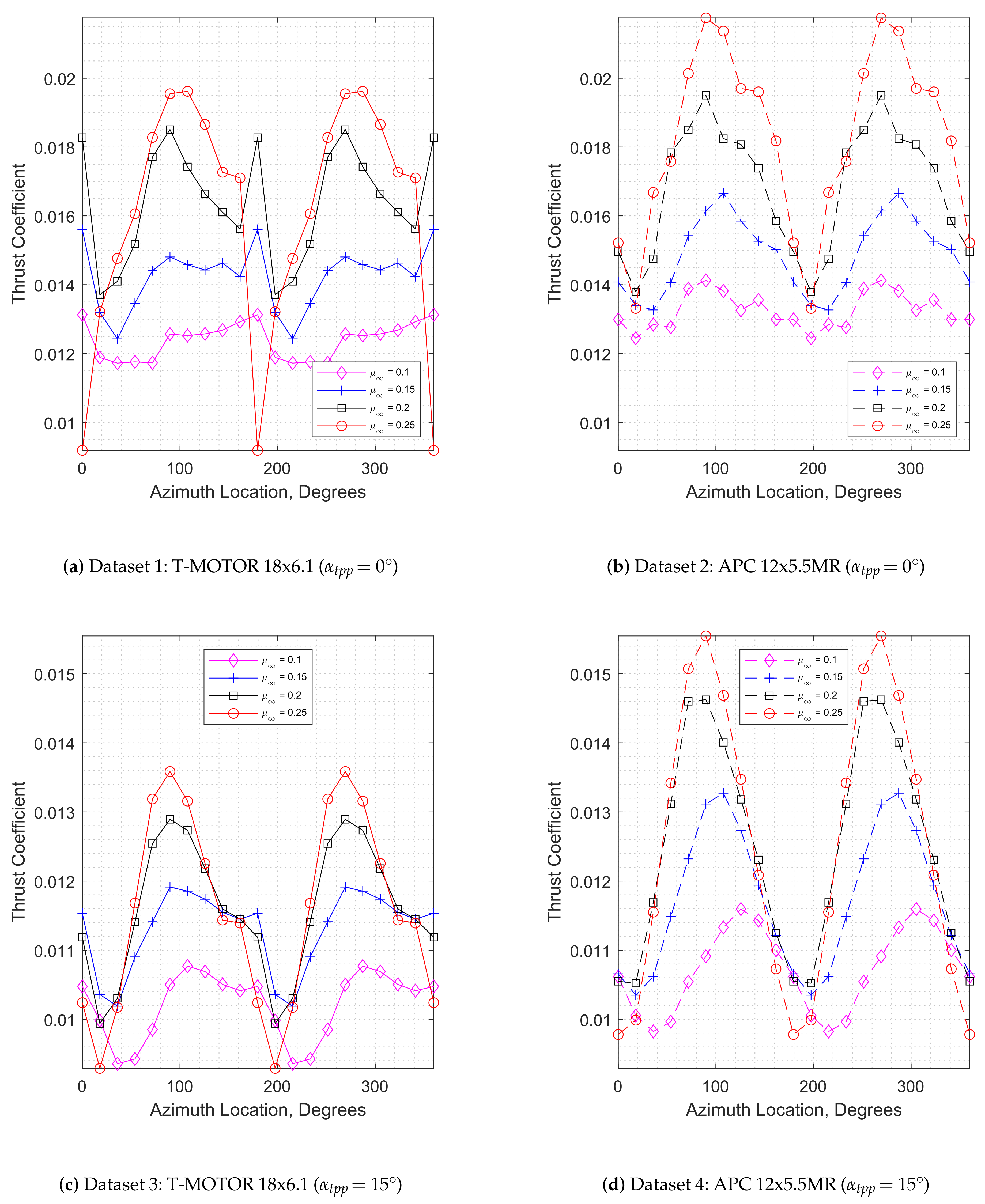
The thrust coefficients versus azimuth locations for each of these four datasets are plotted in Figure 12. In most cases, the peak rotor thrust appears around ψ = 90 110 and 270 290 , which corresponds to a blade passing the region of maximum advancement. The onset of this peak is delayed as the normalized freestream velocity is decreased. For the APC rotor operating at α t p p = 0 , Figure 12b shows that the thrust coefficient for the μ = 0.25 case is equivalent to or greater than that of the μ = 0.2 case across the range of azimuth locations, which is not the case for the other datasets. This results in a higher time-averaged thrust coefficient for the APC rotor at α t p p = 0 and μ = 0.25 , as shown in Figure 11.
Most of the cases shown in Figure 12, except for those shown in Figure 12d, have small secondary peaks occurring roughly 20 50 after the primary peaks. To explain the cause of these peaks, 
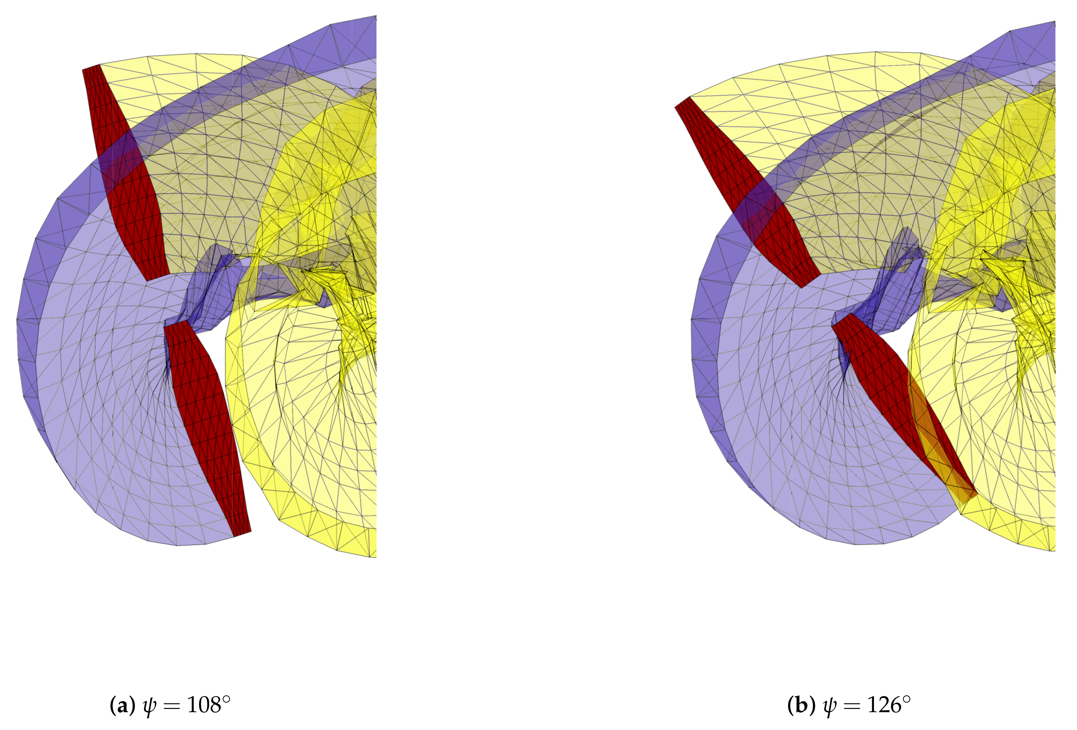
Figure 13 illustrates the APC rotor at two azimuth locations corresponding to a primary and secondary peak for the case of μ = 0.25 in Figure 12b. Figure 13a is a top-down snapshot of the APC rotor during the primary peak at an azimuth location ψ = 108 . At this azimuth location, the shed vortex of a previously advancing blade is passing over the advancing blade. As this tip-vortex moves inboard along the blade, the upwash outside of this tip-vortex increases the effective angle of attack of the blade sections along the outboard portion of the rotor blade. Similarly, at this azimuth location, the retreating blade is outside of the tip-vortex of a previous blade pass, which increases the effective angle of attack of the blade sections along the retreating blade, which are experiencing low relative velocities. The rotor and wake geometry corresponding to the secondary peaks of the case of μ = 0.25 in Figure 12b are displayed in Figure 13b. This figure represents an azimuth location of ψ = 126 . The main difference between Figure 13a,b is that the retreating blade has entered into the tip-vortex of a previous blade pass, indicating that the primary and secondary peaks in the transient thrust for this case could be created by a negative effect acting on the retreating blade caused by this interaction. As the retreating blade enters further into the downwash region, the thrust output of the rotor collapses, leading to the negative thrust peak at ψ = 180 200 .
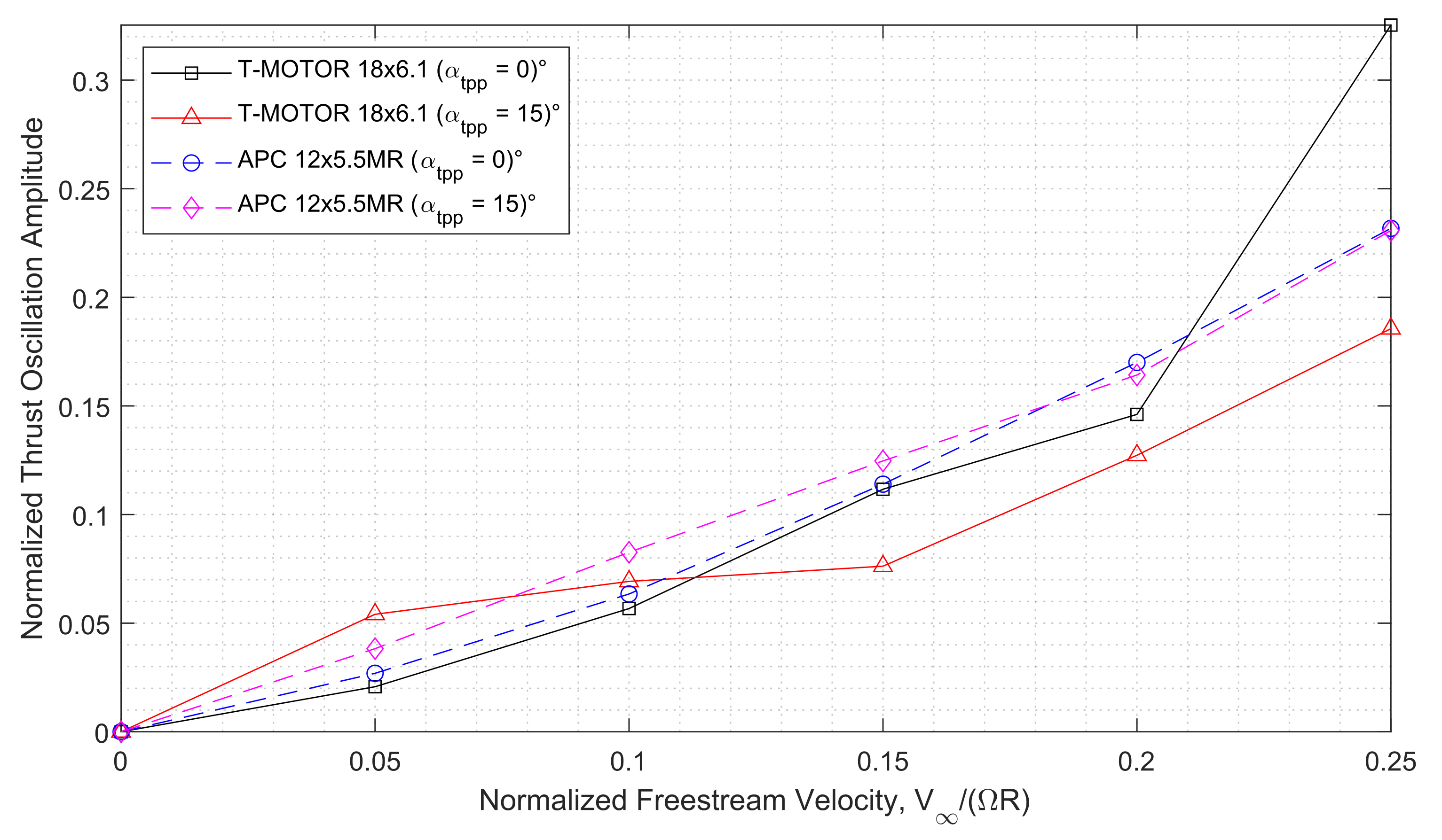
In order to identify further trends in the transient thrust data presented in Figure 12, a normalized thrust coefficient is used:
C ^ T = C T C ¯ T
where C ¯ T represents the mean thrust coefficient as shown in Figure 11. The amplitude of oscillation of this normalized thrust is then:
λ ^ = 1 2 ( C ^ T , m a x C ^ T , m i n ) = C T , m a x C T , m i n 2 C ¯ T
Figure 14 shows this normalized thrust oscillation amplitude λ ^ plotted against the normalized freestream velocity of Equation (3) for all four datasets. As expected, the normalized thrust oscillation amplitude increases with the normalized freestream velocity, as advancing and retreating blade effects become more severe. In the extreme, such as the cases at a normalized freestream velocity of μ = 0.25 , the normalized thrust oscillation amplitude of the rotors is in the range of 20–30% of the mean rotor thrust output, indicating the rotor thrust output varies by 0.4 C ¯ T 0.6 C ¯ T per revolution. The rotor blade design appears to impact the relationship between the normalized thrust oscillation amplitude and the normalized freestream velocity, as evidenced by the differences between the T-MOTOR and APC results, which become more pronounced with an increasing normalized freestream velocity. Observing these four datasets, there does not appear to be a discernible link between the normalized thrust oscillation amplitude and the tip-path plane angles of α t p p = 0 and 15 , though the normalized thrust oscillation amplitude will be zero for all normalized freestream velocities at the tip-path plane angle α t p p = 90 .
Understanding the magnitude of oscillations in the thrust of a rigid rotor provides added context for the rotor designer. The total thrust oscillation amplitude of the rotor in Figure 14 only represents the force oscillations of both blades together and does not represent the thrust oscillation amplitude of a single blade. To begin quantifying the individual blade contributions to the thrust coefficient, two distinct operating conditions were chosen for closer analysis. Figure 15 shows the normalized thrust coefficients of the rotors plotted against azimuth location, including individual blade contributions, for tip-path plane angles of α t p p = 0 and 15 and normalized freestream velocities of μ = 0.25 and 0.1 , respectively. The thrust coefficients were normalized using Equation (7) to allow a direct comparison.
The individual blade contributions for the two fully-edgewise cases in Figure 15a,b vary by approximately 0.7 0.9 C ¯ T over a revolution. In both cases, the peak thrust output of the rotor aligns with the peak thrust output of the advancing blade, which occurs at azimuth locations of approximately 95 for Blade A and 275 for Blade B, for both the T-MOTOR and APC rotors under this operating condition. Figure 15a also shows that the retreating blade of the T-MOTOR rotor is predicted to have its thrust collapse rapidly as the blade passes through the downstream region, likely due to blade–vortex interactions. This contributes to the large overall variation in the normalized thrust oscillation amplitude for this specific rotor and operating condition, as shown in Figure 14. The partially-edgewise cases in Figure 15c,d both have normalized blade thrust contributions varying by approximately 0.6 C ¯ T . Under this specific operating condition, the thrust output of the retreating blade of the T-MOTOR rotor begins to recover faster than the advantage of the advancing blade is lost, leading to a slight double peak in the total thrust output of the rotor.
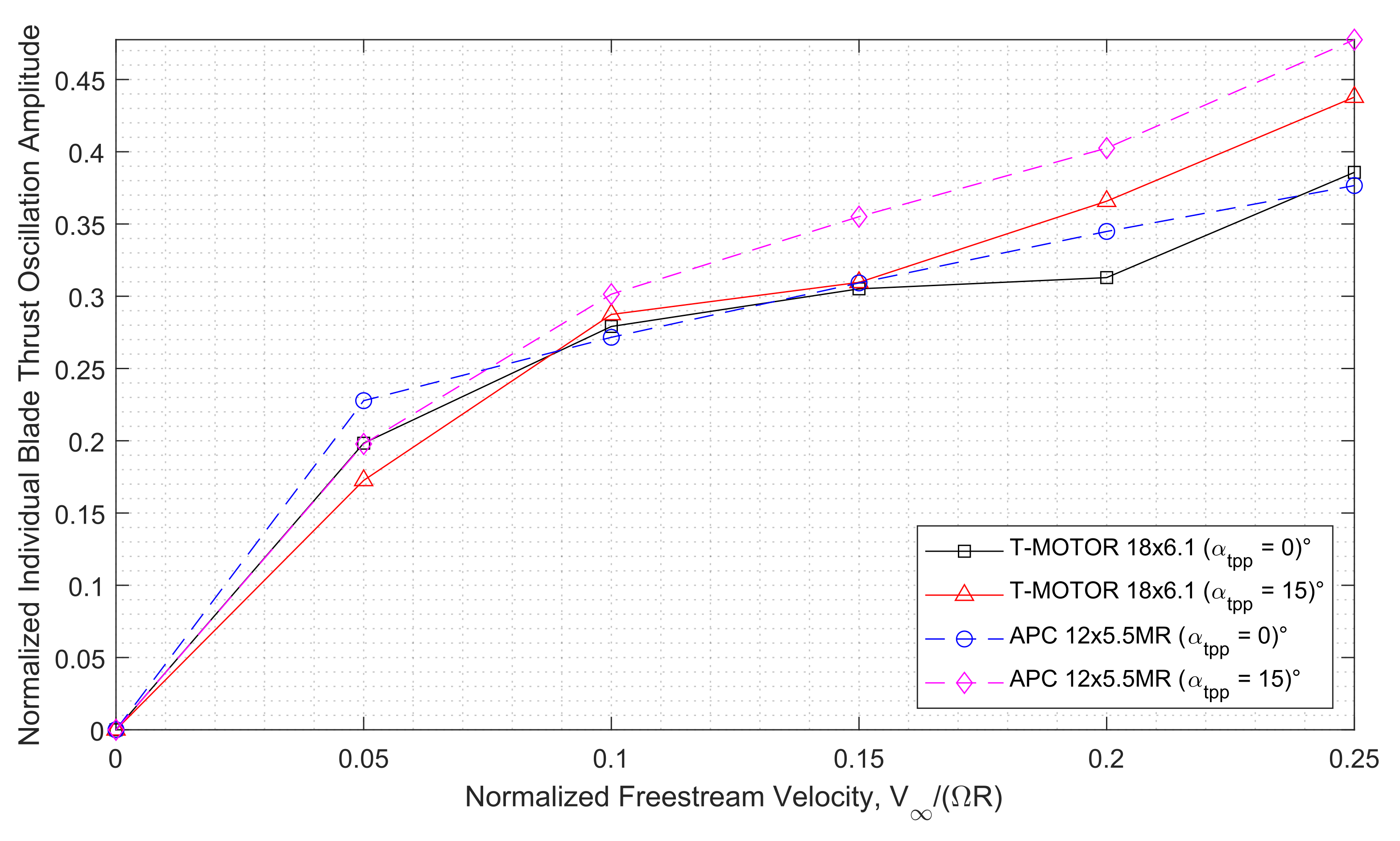
In order to generalize the results shown in Figure 15, normalized individual blade thrust oscillation amplitudes were found for all datasets. These results are shown in Figure 16. Even at low normalized freestream velocities, the oscillation amplitudes for a single rotor blade are approximately 0.2 C ¯ T , with a total variation in thrust output of 40% of the mean rotor thrust. This oscillation amplitude increases to approximately 0.4 C ¯ T as the normalized freestream velocity increases, indicating that the thrust output of a single rotor blade may approach the mean thrust output of the entire rotor over one revolution under these conditions. Analysis of this nature should prove useful when considering aeroelastic, aeroacoustic, and structural properties during the design phase of rigid rotors.
The relationship between the normalized individual blade thrust oscillation amplitude and the normalized freestream velocity does not appear to be linear. In addition, as with the total normalized thrust oscillation amplitude shown in Figure 14, there does not appear to be a discernible pattern between the two tip-path plane angles for each rotor. The exceptions to this are the α t p p = 15 cases at high normalized freestream velocities, where the normalized individual blade thrust oscillation amplitude exceeds those of the fully-edgewise cases. This is likely due to how the mean rotor thrust changes with the normalized freestream velocity. Figure 11 shows that as the normalized freestream velocity increases, the thrust output of the rotors at α t p p = 0 increases at a greater rate than at α t p p = 15 . However, advancing and retreating blade effects become more severe as the normalized freestream velocity increases, which leads to higher normalized individual blade thrust oscillation amplitudes for α t p p = 15 , as the mean thrust output of the rotor does not change significantly. Coupled with the fact that these oscillation values should approach zero as the tip-path plane angle of attack approaches 90 , it is likely that α t p p = 0 15 represents the tip-path plane angle of attack region that results in the highest normalized individual blade thrust oscillation amplitudes for these two rotors.
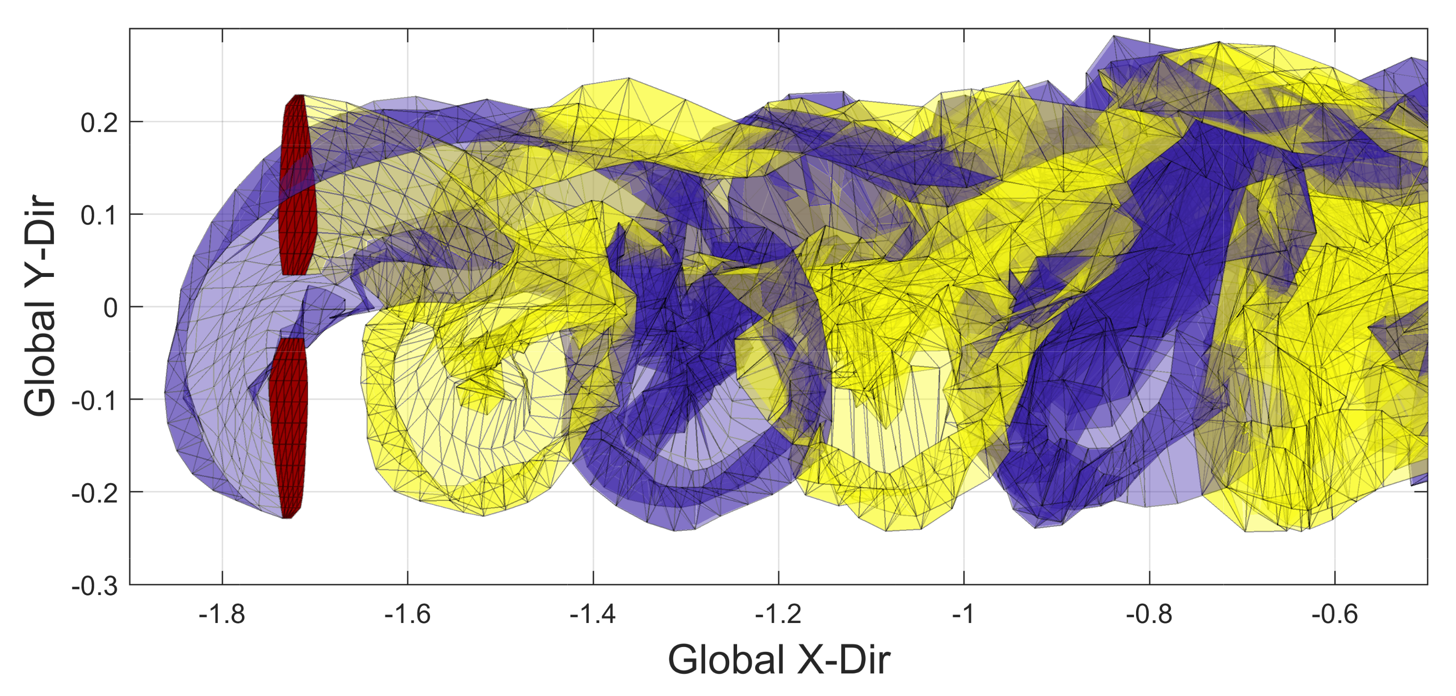
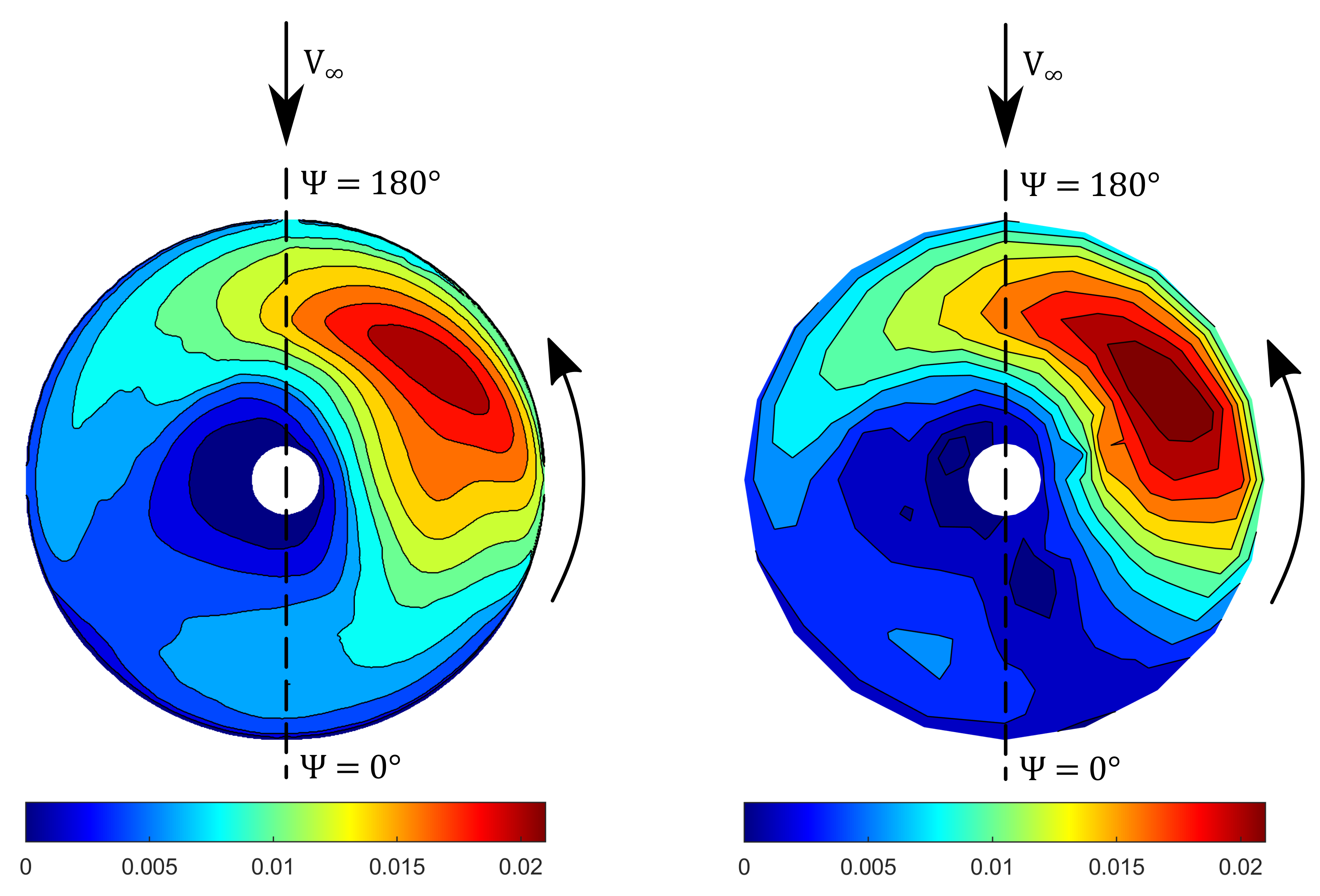
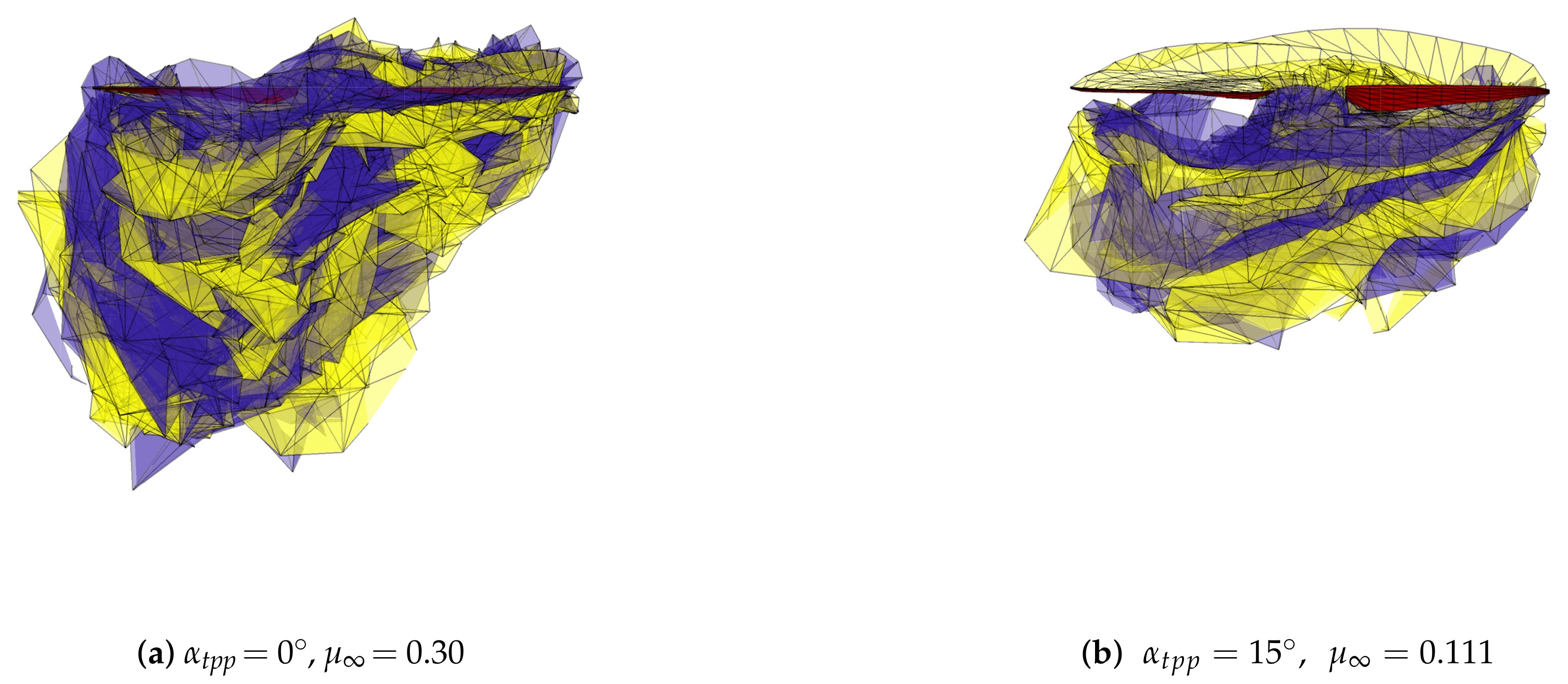
Another important takeaway from this analysis is an apparent asymmetry in the wake structure behind a rigid rotor in forward flight, which was noted by Misiorowski et al. [5]. Figure 17 provides frontal views of two T-MOTOR 18x6.1 cases, with Figure 17a representing the rotor in fully-edgewise flow at a high normalized freestream velocity and Figure 17b representing the rotor at a tip-path plane angle of α t p p = 15 at a more modest normalized freestream velocity. Due to the higher blade thrust oscillation amplitude present in the fully-edgewise case, the wake structure is highly asymmetric, with a large increase in downwash behind the advancing blade where the individual blade thrust output is the highest. The wake of the rotor in Figure 17b, however, is more uniform, but still exhibits some degree of asymmetry. This asymmetric wake structure is in conflict with Glauert’s assumption that a rotor in high-speed forward flight has an induced downwash similar to that of a circular wing, as discussed by Leishman [31], implying that this assumption is not necessarily valid for rigid rotors. Knowing the wake structure behind a rigid rotor in forward flight may be of use to multicopter designers when considering rotor–wake interactions, such as determining the optimal rotation directions of the rotors or the best orientation of the vehicle for forward flight. Research of this nature has been conducted by Barcelos et al. [33] and Misiorowski et al. [5].

4. Conclusions

The purpose of this research was to quantify the transient thrust output of rigid rotors in forward flight, using computational modeling substantiated through wind-tunnel experimentation and CFD validation. The potential-flow based computation model used in this study is based on distributed doublet elements (DDEs) and is well-suited to unsteady analyses with relaxed wakes. When compared to experimentally-obtained time-averaged thrust coefficients for a small rigid rotor, the DDE-based method showed good agreement at various normalized freestream velocities and tip-path plane angles. In comparison with the transient CFD analysis of a small rigid rotor in forward flight, the DDE-based method showed good agreement with the maximum and minimum sectional thrust coefficients and their respective azimuth locations.
Two small rigid rotors were then analyzed at various forward-flight operating conditions. Apart from the peaks and troughs in the transient thrust coefficient due to advancing and retreating blade velocity effects, wake effects acting on the rotor blades were also shown to affect the transient thrust coefficient under certain operating conditions. Additionally, the analysis indicates that the wake structure behind a rigid rotor in forward flight is asymmetric. The increased thrust output of the advancing blade leads to a wake structure that is convected farther away from the rotor disk on the advancing side.
A normalized thrust oscillation amplitude was introduced to quantify the oscillations in the transient thrust coefficient. For both of the rotors, the predicted transient thrust oscillation amplitudes varied from 0.05 0.3 C ¯ T for tip-path plane angles of attack of 0 and 15 across a range of normalized freestream velocities, indicating that the transient thrust of a rotor may vary by approximately 60% of the mean rotor thrust per revolution. The predicted individual blade thrust oscillation amplitudes ranged from 0.15 0.45 C ¯ T , meaning that it is not uncommon for the thrust output of a single blade to vary by a value in the same order as the mean thrust of the rotor. Differences in the relationship between the normalized thrust oscillation amplitude and the normalized freestream velocity for the two rotors indicates that blade design plays an important role in the thrust oscillation of the rotor as the forward speed changes.

Author Contributions

Conceptualization, T.K., G.B. and J.C.; methodology, T.K., G.B. and J.C.; software, T.K.; validation, T.K., G.B. and J.C.; formal analysis, T.K.; investigation, T.K., G.B. and J.C.; data curation, T.K.; writing—original draft preparation, T.K.; writing—review and editing, G.B. and J.C.; visualization, T.K.; funding acquisition, G.B. All authors have read and agreed to the published version of the manuscript.

Funding

This research was funded in part by the Natural Sciences and Engineering Research Council of Canada (NSERC) [funding reference number RGPIN-2016-03920].

Acknowledgments

This research was made possible through support from Compute Canada.

Conflicts of Interest

The authors declare no conflict of interest.

Abbreviations

The following abbreviations are used in this manuscript:
C T Thrust coefficient
C ¯ T Mean thrust coefficient
C ^ T Normalized thrust coefficient
cChord length
DDiameter
D D E Distributed doublet element
JPropeller advance ratio
MNumber of chordwise elements
nRevolutions per second
VVelocity
V Freestream velocity
α t p p Rotor tip-path plane angle of attack
Γ Circulation
Δ x c Chord length of a DDE element
Δ x w Distance traveled by lifting surface in one timestep
λ ^ Normalized thrust oscillation amplitude
μ Rotor advance ratio
μ Normalized freestream velocity

References

  1. Brandt, J.B. Small-Scale pRopeller Performance at Low Speeds. Ph.D. Thesis, University of Illinois at Urbana-Champaign, Champaign, IL, USA, 2005. [Google Scholar]
  2. University of Illinois at Urbana-Champaign, Department of Aerospace Engineering. UIUC Propeller Data Site. 2015. Available online: https://m-selig.ae.illinois.edu/props/propDB.html (accessed on 3 November 2018).
  3. Kolaei, A.; Barcelos, D.; Bramesfeld, G. Experimental analysis of a small-scale rotor at various inflow angles. Int. J. Aerosp. Eng. 2018, 2018, 2560370. [Google Scholar] [CrossRef] [Green Version]
  4. Serrano, D.; Ren, M.; Qureshi, A.J.; Ghaemi, S. Effect of disk angle-of-attack on aerodynamic performance of small propellers. Aerosp. Sci. Technol. 2019, 92, 901–914. [Google Scholar] [CrossRef]
  5. Misiorowski, M.; Gandhi, F.; Oberai, A.A. Computational Study on Rotor Interactional Effects for a Quadcopter in Edgewise Flight. AIAA J. 2019, 57, 5309–5319. [Google Scholar] [CrossRef] [Green Version]
  6. Carroll, T. A Design Methodology for Rotors of Small Multirotor Vehicles. Master’s Thesis, Ryerson University, Toronto, ON, Canada, 2015. [Google Scholar]
  7. Katz, J.; Plotkin, A. Low-Speed Aerodynamics; Cambridge Aerospace Series; Cambridge University Press: Cambridge, UK, 2001. [Google Scholar]
  8. Murua, J.; Palacios, R.; Graham, J.M.R. Assessment of wake-tail interference effects on the dynamics of flexible aircraft. AIAA J. 2012, 50, 1575–1585. [Google Scholar] [CrossRef] [Green Version]
  9. Nguyen, A.T.; Kim, J.K.; Han, J.S.; Han, J.H. Extended unsteady vortex-lattice method for insect flapping wings. J. Aircr. 2016, 53, 1709–1718. [Google Scholar] [CrossRef]
  10. Simpson, R.J.; Palacios, R.; Murua, J. Induced-drag calculations in the unsteady vortex lattice method. AIAA J. 2013, 51, 1775–1779. [Google Scholar] [CrossRef] [Green Version]
  11. Tan, J.F.; Sun, Y.M.; Barakos, G.N. Vortex Approach for Downwash and Outwash of Tandem Rotors in Ground Effect. J. Aircr. 2018, 55, 2491–2509. [Google Scholar] [CrossRef] [Green Version]
  12. Tan, J.F.; Wang, H.W. Simulating unsteady aerodynamics of helicopter rotor with panel/viscous vortex particle method. Aerosp. Sci. Technol. 2013, 30, 255–268. [Google Scholar] [CrossRef]
  13. Singh, P.; Friedmann, P.P. Application of vortex methods to coaxial rotor wake and load calculations in hover. J. Aircr. 2018, 55, 373–381. [Google Scholar] [CrossRef]
  14. Hirato, Y.; Shen, M.; Gopalarathnam, A.; Edwards, J.R. Vortex-sheet representation of leading-edge vortex shedding from finite wings. J. Aircr. 2019, 56, 1626–1640. [Google Scholar] [CrossRef]
  15. Saberi, H.; Khoshlahjeh, M.; Ormiston, R.A.; Rutkowski, M.J. Overview of RCAS and application to advanced rotorcraft problems. In Proceedings of the American Helicopter Society 4th Decennial Specialists’ Conference on Aeromechanics, San Francisco, CA, USA, 21–23 January 2004. [Google Scholar]
  16. Johnson, W. Rotorcraft aerodynamics models for a comprehensive analysis. Annual Forum Proceedings of the American Helicopter Society. Am. Helicopter Soc. 1998, 54, 71–94. [Google Scholar]
  17. Russell, C.R.; Sekula, M.K. Comprehensive Analysis Modeling of Small-Scale UAS Rotors. In Proceedings of the AHS International 73rd Annual Forum, Fort Worth, TX, USA, 9–11 May 2017. [Google Scholar]
  18. Leishman, J.G.; Bhagwat, M.J.; Bagai, A. Free-vortex filament methods for the analysis of helicopter rotor wakes. J. Aircr. 2002, 39, 759–775. [Google Scholar] [CrossRef]
  19. Govindarajan, B.; Leishman, J. Curvature corrections to improve the accuracy of free-vortex methods. J. Aircr. 2016, 53, 378–386. [Google Scholar] [CrossRef]
  20. Barcelos, D.; Kolaei, A.; Bramesfeld, G. Aerodynamic Interactions of Quadrotor Configurations. J. Aircr. 2020, 57, 1074–1090. [Google Scholar] [CrossRef]
  21. Bramesfeld, G.; Maughmer, M. Relaxed-wake vortex-lattice method using distributed vorticity elements. J. Aircr. 2008, 45, 560–568. [Google Scholar] [CrossRef]
  22. ATI Industrial Automation. F/T Sensor: Mini45. 2019. Available online: https://www.ati-ia.com/Products/ft/ft_models.aspx?id=Mini45 (accessed on 5 June 2017).
  23. Krebs, T. A Distributed Doublet-Based Method for Unsteady Aerodynamic Analysis with Relaxed Wakes. Ph.D. Thesis, Ryerson University, Toronto, ON, Canada, 2021. [Google Scholar]
  24. Drela, M. Flight Vehicle Aerodynamics; MIT Press: Cambridge, MA, USA, 2014. [Google Scholar]
  25. Johnson, F. A General Panel Method for Analysis and Design of Arbitrary Configurations in Incompressible Flows; NASA CR-3079; Boeing Airplane Company: Chicago, IL, USA, 1980. [Google Scholar]
  26. Ashby, D.L.; Dudley, M.R.; Iguchi, S.K.; Browne, L.; Katz, J. Potential Flow Theory and Operation Guide for the Panel Code PMARC. 1991. Available online: https://ntrs.nasa.gov/citations/19920023178 (accessed on 12 May 2018).
  27. Murua, J. Flexible Aircraft Dynamics with a Geometrically-Nonlinear Description of the Unsteady Aerodynamics. Ph.D. Thesis, Imperial College London, London, UK, 2012. [Google Scholar]
  28. Simpson, R.J.; Palacios, R. Numerical aspects of nonlinear flexible aircraft flight dynamics modeling. In Proceedings of the 54th AIAA/ASME/ASCE/AHS/ASC Structures, Structural Dynamics, and Materials Conference, Boston, MA, USA, 8–11 April 2013; p. 1634. [Google Scholar]
  29. Rusak, Z.; Wasserstrom, E.; Seginer, A. Convergence characteristics of a vortex-lattice method for nonlinear configuration aerodynamics. J. Aircr. 1985, 22, 743–749. [Google Scholar] [CrossRef]
  30. Cole, J.A.; Maughmer, M.D.; Bramesfeld, G.; Melville, M.; Kinzel, M. Unsteady Lift Prediction with a Higher-Order Potential Flow Method. Aerospace 2020, 7, 60. [Google Scholar] [CrossRef]
  31. Leishman, J. Principles of Helicopter Aerodynamics; Cambridge Aerospace Series; Cambridge University Press: Cambridge, UK, 2002. [Google Scholar]
  32. Kayran, A. Küssner’s Function in the Sharp Edged Gust Problem-A Correction. J. Aircr. 2006, 43, 1596–1599. [Google Scholar] [CrossRef]
  33. Barcelos, D.F.; Kolaei, A.; Bramesfeld, G. Performance prediction of multirotor vehicles using a higher order potential flow method. In Proceedings of the 2018 AIAA Aerospace Sciences Meeting, Kissimmee, FL, USA, 8–12 January 2018; p. 1528. [Google Scholar]
Figure 1. Ryerson University’s subsonic wind-tunnel [3].
Aerospace 09 00028 g001
Figure 2. The rotor-test stand configuration and angle of attack convention. (a) The rotor-test stand. (b) Definition of tip-path plane angle of attack [3].
Aerospace 09 00028 g002
Figure 3. Comparison between UIUC and RU wind-tunnel test data for the Master Airscrew 11x7E propeller.
Aerospace 09 00028 g003
Figure 4. T-MOTOR 18x6.1 rotor geometry [3].
Aerospace 09 00028 g004
Figure 5. An overview of the DDE method.
Aerospace 09 00028 g005
Figure 6. A top-down view of a DDE in the local coordinate system.
Aerospace 09 00028 g006
Figure 7. DDE prediction of lift response of a 2D wing section as it encounters a sharp-edged gust.
Aerospace 09 00028 g007
Figure 8. Top-down view of a rotor in fully-edgewise flow using a relaxed-wake model.
Aerospace 09 00028 g008
Figure 9. Comparison of time-averaged thrust forces for various advance ratios and angles of attack.
Aerospace 09 00028 g009
Figure 10. Sectional thrust coefficient d C T / d ( r / R ) predictions for α t p p = 5 , μ = 0.162 . (a) CFD predictions [5]. (b) DDE metond predictions.
Aerospace 09 00028 g010
Figure 11. Thrust coefficient vs. normalized freestream velocity as predicted with the DDE method.
Aerospace 09 00028 g011
Figure 12. Thrust coefficient vs. azimuth location as predicted with the DDE method.
Aerospace 09 00028 g012
Figure 13. Rotor and wake visualization of the APC 12x5.5MR ( α t p p = 0 , μ = 0.25 ) as modeled in the DDE method.
Aerospace 09 00028 g013
Figure 14. Normalized thrust oscillation amplitude vs. normalized freestream velocity as predicted with the DDE method.
Aerospace 09 00028 g014
Figure 15. Individual blade contributions to thrust coefficient as predicted with the DDE method.
Aerospace 09 00028 g015
Figure 16. Normalized single blade thrust oscillation amplitude vs. normalized freestream velocity as predicted with the DDE method.
Aerospace 09 00028 g016
Figure 17. Frontal view of a T-MOTOR 18x6.1 and wake as modeled in the DDE method.
Aerospace 09 00028 g017
Publisher’s Note: MDPI stays neutral with regard to jurisdictional claims in published maps and institutional affiliations.

