Article

Task Parameter Planning Algorithm for UAV Area Complete Coverage in EO Sector Scanning Mode

1
Aviation University of Air Force, Changchun 130022, China
2
The Representative Office of Air Force in Luoyang, Luoyang 471000, China
*
Author to whom correspondence should be addressed.
Aerospace 2023, 10(7), 612; https://doi.org/10.3390/aerospace10070612
Submission received: 23 April 2023 / Revised: 28 June 2023 / Accepted: 29 June 2023 / Published: 3 July 2023
(This article belongs to the Special Issue Applications of Drones (Volume II))

Abstract

:
When Unmanned Aerial Vehicles (UAVs) are used in search and rescue operations, electro-optical (EO) devices are usually used as the detection equipment, and area coverage is used as the main search method. However, the sector scanning mode of EO puts forward higher requirements for task parameter planning. First, to ensure there is no missing coverage, a method to determine the full coverage width of EO equipment in sector scanning mode is proposed. Second, the constraint of no interval missing and the model of the speed-to-high ratio constraint are established, and the constraints of other factors are addressed in the context of the problem situation. Third, a coverage efficiency index is proposed for the boustrophedon coverage of a rectangular area, and a comprehensive coverage index is established. Finally, task parameter planning algorithms are designed, based on Immune Algorithm (IA), Grey Wolf Optimization (GWO) and Variable Neighborhood Search (VNS), respectively. The simulation results showed that the designed algorithms, based on IA, GWO and VNS, can effectively solve task planning problems. In general, IA is more suitable for offline occasions, VNS is suitable for online real-time planning, and GWO has characteristics between the two. The coverage process, based on optimized parameters, meets all constraints, has higher search efficiency and does not miss areas, proving the correctness of these models and the effectiveness of the planning algorithm. The research presented in this paper provides a technical basis for efficient and fully automated target search and rescue.

1. Introduction

The search and rescue problem has always existed along with the development of society, and it is also a long-term challenge. Traditional search and rescues are mainly implemented with the utilization of manned aircraft, helicopters, ships, etc. In recent years, with the increasing maturity of Unmanned Aerial Vehicles (UAVs) and photoelectric sensors, search and rescue operations based on UAV have proven feasible and have been successfully tested and applied [1,2,3], showing advantages of large range, strong timeliness, low risk and low economic cost.
Area complete coverage search is a commonly used search and rescue method for UAVs [4] and is suitable for maritime rescue [5], disaster rescue [6], and for use in mountainous areas [7]. In addition, area coverage search can also be used for regional investigation [8], patrol and surveillance [9], infrastructure inspection [10], precision agriculture [11,12] and other scenarios. Consequently, it has become an important research direction for UAV applications. The goal of area coverage is to cover the entire area of interest, while minimizing the time and distance spent on covering routes [13].
In a UAV area coverage search, electro-optical (EO) equipment is typically used for detection. EO equipment has advantages of high resolution and long detection distances, but the disadvantage is that the fixed field of view is relatively small. Therefore, to improve search efficiency, operators control the EO device to perform sector scanning relative to the aircraft body. This usage greatly increases the coverage width of UAV during a single route, but also puts higher requirements on mission parameter planning, such as balancing the limitations of the UAV platform, EO device, environmental conditions, and operators to maximize the execution efficiency of the mission process. This has become a difficult and valuable issue for users.
At present, many studies on UAV area coverage have focused on route planning algorithms, mainly focusing on the effective planning of covered routes in complex areas. For areas with regular shapes, such as rectangles, no decomposition is required. Simple path planning is sufficient for complete coverage without overlapping. A typical example is the boustrophedon method, which is a route pattern that simply moves back and forth along the longest side of a polygon [14,15].
For areas with irregular shapes, most area coverage route planning algorithms decompose the target area into subunits. For example, Choset proposed an approximate cell decomposition method [16], which decomposes the generated grid map into smaller sub-maps and then generates the navigation trajectory covering the entire area, according to the density of obstacles in each sub-map. Other similar decomposition methods include cell-based [17], Morse-based [18], wavefront-based [19], and neural network-based [20]. On the basis of decomposition, further path planning to cover the area can be performed. For example, ref. [21] proposed a new method based on ant colony optimization (ACO) to determine the trajectory of a UAV that can strike a balance between the calculation requirements and the quality of the trajectory plan. A new coverage flight path planning algorithm, based on the ACO algorithm, was also designed in [22], which can find collision-free, minimum-length flight paths for UAV in a three-dimensional (3D) urban environment with fixed obstacles. Other algorithms used for UAV coverage route planning include the constrained differential evolution [23], grey wolf optimizer [24], and hybrid algorithms [25]. A real-time path-planning solution for an area-coverage mission using multiple cooperative UAVs was proposed in [26]. The experimental results showed that the probability of achieving a 50% success rate with three UAVs is 2.35 times faster than that with one UAV. Given the limited capabilities of a single UAV, it is sometimes necessary for multiple UAVs to collaborate to complete a certain task, which can significantly improve coverage efficiency and provide better timeliness. Leader–follower [27] is an effective route planning method for multi-UAV formation flight.
In the aforementioned studies, the coverage width of the search equipment is usually set as a constant, and route planning is carried out accordingly, without considering the influence of EO equipment resolution, scan mode, and other factors on coverage width and route planning.
A brief model of EO coverage width was established in some studies, wherein the influence of factors, such as flight height, on coverage width was initially considered, and a comprehensive study was conducted by combining a route planning algorithm. For example, in [28,29,30], the geometric relationship between the static detection width of the UAV detector and flight height, pitch angle, and search azimuth angle was preliminarily studied. Avellar [31] calculated the coverage width of the camera according to the width of the field of view of the image sensor, focal length of the camera lens, and distance H (flight height) between the camera and ground. Di Franco [32] calculated the optimal motion trajectory and maximum height according to the distance of ground samples (image resolution) and proposed an energy-saving round-trip complete coverage algorithm to minimize the number of turns and, thus, improve task efficiency. However, these models of coverage width do not consider limitations and influencing factors, such as target recognition, velocity-to-height ratio, scan omission, and field-of-view distortion. Generally, they differ significantly from the actual situation, and cannot reflect the actual situation in practice.
Some scholars have promoted the application of computer vision in search tasks to reduce the workload of mission personnel and have even promoted the development of fully autonomous UAVs for search missions [33,34]. Experiments have begun on UAVs equipped with perception components based on deep neural networks (DNN). In [35], DNN models that were pre-trained in different fields were proposed for UAVs, one for detecting human joints, and the other for measuring the similarities in appearance between two images in pedestrian tracking to solve the tracking problem. In [36], the limitation of time for search and rescue missions was emphasized, and the embedded system, which is based on deep learning technology, can detect swimmers in open waters, thus enhancing the combat ability of emergency personnel. Combined with global navigation satellite system (GNSS) technology, it can be used for accurate human detection and rescue equipment release. In [37], a camera-based UAV system for automatic target positioning was developed. By setting reasonable pigment thresholds, the automatic recognition of red and blue targets in aerial images was realized, providing useful insights for exploration in automatic target recognition. It should be pointed out that fully autonomous UAVs for search missions undoubtedly represent the trend of the future. However, although this progress improves identification efficiency, it also has higher requirements for no-omission coverage.
According to the literature searched, research on parameter planning of complete area coverage tasks in the EO sector scanning mode is still lacking.
Furthermore, task parameter planning for sector scanning involves many factors and needs to consider requirements and constraints from the perspective of many aspects, which is a typical multi-objective optimization problem. Many effective algorithms have been developed for different multi-objective optimization problems. Exhaustive search techniques can solve discrete optimization problems, but the computational cost is high when the variable space is large [38]. Scenario-based robust optimization can ensure better optimization robustness under the premise of achieving optimization objectives, such performance being crucial for uncertain environments [39]. Heuristic search algorithms have high efficiency but can only obtain suboptimal solutions [40]. Some new bionic heuristic algorithms, such as Gray Wolf Optimization (GWO) [41,42] and Particle Swarm Optimization (PSO) [43], have similar characteristics. The Genetic Algorithm (GA) [44] is suitable for almost all optimization problems, but requires a large amount of computation and is generally used in offline situations. The Immune Algorithm (IA) [45] retains the evolutionary mechanism of GA, and at the same time has a unique concentration inhibition mechanism, which better overcomes the problem of local optimization, but has the disadvantage of high computational cost. The Variable Neighborhood Search (VNS) [46] and Multistage Neighborhood Search (MNS) [47] algorithms overcome the local search limitation of Neighborhood Search (NS) and can search the solution space in multiple different neighborhoods, so they have good global search ability. The implementation of the algorithm is relatively simple. However, its convergence accuracy depends on the design of neighborhood operators and the setting of the algorithm parameters, which requires users to have a certain amount of professional experience. Therefore, it is necessary to develop an efficient and high-precision optimization algorithm for this problem. In the study here presented, the representative IA, GWO, and VNS algorithms were used to solve the task planning problem, and the convergence performance and computing efficiency of different optimization algorithms compared, providing a useful reference for solving the problem.
In general, there are several problems in the current research, as follow:
  • Most research on UAV coverage focuses on route planning algorithms, and the processing of EO equipment factors is too simple, or is even ignored, which does not reflect the actual situation.
  • There is a lack of research on area-coverage task planning in the sector scanning mode of UAV EO equipment. There is not only a lack of descriptive model research for the problem but also a lack of task planning research combining the problem model and optimization algorithm.
In view of this, the objectives of this paper follow:
  • A no-omission coverage width model was established for the sector scanning of UAV EO equipment that considers the influence of target recognition.
  • Description models of the constraints were established that, combined with the sector scanning method, consider the influence of various constraints on parameter planning of the area coverage task. Such as target recognition, speed-to-height ratio, and missed scanning, etc.
  • A parameter planning algorithm to address the area coverage task in the sector scanning mode was designed to ensure an efficient search, based on the representative IA, GWO, and VNS algorithms, and combined with constraints.
  • The three designed task planning algorithms were simulated and verified, and the main performances of these algorithms in solving the problems in this study were compared.

2. Coverage Width Modeling

2.1. Scanning Mode of the UAV EO Equipment

There are a variety of scanning modes for the UAV EO equipment, such as side scan, cone scan, and sector scan. In this study, the most common and complex sector scanning mode was investigated, and the other modes regarded as a special case of the sector scanning mode.
As shown in Figure 1, it was assumed that the UAV maintains horizontal flight. In sector scanning mode, the pitch angle μ of the EO equipment view field remains unchanged, and the azimuth angle θ of the field of view scans back and forth at a constant speed within an angular range [ θ , θ ].

2.2. Model of Static View Field of EO Equipment

In the sector scanning mode, there are two types of view fields of the EO equipment: scanning view field and static view field. The static view field is the inherent angle of view of EO equipment, and the scanning view field is the detectable range of the static view field during scanning mode, which is related to the static view field and the scan azimuth angle θ .
As shown in Figure 2, O 1 represents the position of the EO equipment, its projection on the ground is O , and its flying height is h . A coordinate system is established with O as the origin, the O X axis is the projection direction of the central axis of the view field on the ground, and the O Y axis is the vertical upward direction. The O Z axis is determined according to the right-hand rule.
As shown in Figure 2, if ε is used to represent the static view field angle of the EO equipment, then μ 1 and μ 2 are the pitch angles of the inner and outer edges of the view field, respectively.
μ 2 = μ 1 + ε
Generally, to find a target in a certain area, we need to ensure two points [48]: first, that the target area is completely scanned without missing data, ensuring that when the field of view scans the target, the target can be identified and found. The problem of target recognition is related to many factors, including the ability of the searcher, environmental factors, and the characteristics of the target itself [49]. Therefore, it needs to be studied by combining theory and practice, and is not addressed in this study. However, to reflect the impact of the target recognition problem on task planning, a target recognition distance threshold d S h B was set in this study. When the target distance is less than d S h B , the target can be recognized; otherwise, it is missed. The distance d S h B comprehensively represents the influence of weather visibility, target characteristics, and EO resolution on the target recognition problem, which limits task parameter planning during coverage search tasks.
As shown in Figure 2, the larger the pitch Angle u is, the larger the area covered by the static view field is, but this also brings adverse effects, including image resolution reduction, graphic distortion aggravation, and so on, affecting the target recognition. Therefore, the pitch Angle μ 2 must be limited. In the region ABCD covered by the static view field, point B is the furthest position away from the EO device. When the target is located at point B, it is the most difficult to identify. Therefore, when the flight altitude is constant, it can be considered that, when the length of OB is equal to d S h B , it is the maximum allowable pitch Angle of EO for target recognition. Therefore, the following equation must be satisfied:
O 1 A = O 1 B d S h B
Threshold d S h B needs to be determined in advance according to weather conditions, target characteristics, and EO equipment recognition pixels, combined with the experience of task operators.
The region formed by the four points of A, B, C and D is the coverage area of the static view field of the EO equipment. It can be seen that the area is not a rectangle, but a trapezoid. For subsequent optimization calculations, each side of the region must be determined.
When O 1 A = O 1 B = d S h B , the maximum static coverage region can be obtained, and the reliable recognition of the target guaranteed, which is beneficial in improving the search efficiency; thus, O 1 A = O 1 B = d S h B can be set.
The four sides are represented as lAB, lBC, lCD, lAD, and lBC = lAD. In triangle O 1 A E 1 , it can be deduced that:
l A B = 2 d S h B sin ε 2
Similarly, in triangle O 1 O A , using the trigonometric function, it can be deduced that:
l O A = ( d S h B ) 2 h 2
μ 2 = arccos ( h / d S h B )
Using Equations (1) and (5), μ 1 can be obtained. In the triangle O 1 O D , it can be deduced that:
l O D = h tan μ 1
l O 1 D = h / cos μ 1
l C D and l A D are obtained as:
l C D = 2 l O 1 D sin ε 2
l A D = l O A l O D

2.3. Complete Coverage Width Modeling

Complete coverage of the target area is a prerequisite for target identification. Therefore, a reasonable determination of the EO coverage width is of great significance to ensure an effective search success rate and to improve search efficiency.

2.3.1. Problem Description

As shown in Figure 2, l O A and l O D are defined as the outer radius R 2 and inner radius R 1 of the static coverage region, respectively.
R 2 = ( d max S h B ) 2 h 2
R 1 = h tan ( arctan ( R 2 / h ) ε )
As shown in Figure 3, V is defined as the flight speed, and it is assumed that the rotational angular velocity of the optical axis of the EO equipment in the horizontal plane is ω . When the EO equipment rotates and scans in the horizontal plane, the pitch angle µ of the optical axis of the field of view remains unchanged.
We define a process in which the static coverage region moves from the leftmost end (position “A1B1C1D1”) to the rightmost end (position “A2B2C2D2”), and then back to the leftmost end (position “A3B3C3D3”) as a scanning cycle. The scanning cycle time is denoted by T.
T = 4 ( θ 1 ε / 2 ) / ω
θ 1 is the scan azimuth.
In a scanning cycle, the UAV flies from O 1 to O 3 , The distance between O 1 and O 3 is represented by l O 1 O 3 , then:
l O 1 O 3 = V T
In a scanning cycle, the EO completes the scanning of two circular arc areas; the area scanned clockwise is indicated by the red line, and the area scanned counterclockwise is indicated by the blue line.
The reachable search width is represented by d .
d = 2 R 2 sin θ 1
However, because the UAV is in continuous flight, there is a “missing area” between the two scan areas in the direction of the maximum value of the dynamic search azimuth, as shown in Figure 3.
Therefore, the search width must be appropriately reduced to exclude the “missing area” to ensure that there are no missing searches. If the innermost point of the “missing area” is represented by P 1 , a parallel line parallel to the flight direction through P 1 is drawn, and the parallel line is the maximum range that can be guaranteed to search without omission.
Let d 1 represent the coverage width of the complete search, related to factors such as UAV flying speed V , photoelectric equipment scanning angular velocity ω , static field of view ε , search azimuth θ 1 , inner/outer radius of the static coverage region R 1 and R 2 , etc. It is necessary to comprehensively consider many factors to determine d 1 .
First, a two-dimensional ground-level coordinate system is established with O 1 as the origin, the flying direction as the Y axis, the X axis perpendicular to the Y axis, and the right direction as positive. The intersection of trajectory B 1 B 2 and straight-line L O 3 B 3 is the position of point P 1 . In the coordinate system O 1 X Y , the point P 1 can be expressed as ( x P 1 , y P 1 ) . Then:
d 1 = 2 | x P 1 |
To solve point P 1 , it is necessary to establish a mathematical equation of trajectory B 1 B 2 and straight-line L O 3 B 3 .

2.3.2. Equation of Trajectory B 1 B 2

The time was set to 0 when the UAV was at O 1 , and B 1 was set as the starting point of the trajectory. In the coordinate system O 1 X Y , since the static coverage region moves in a uniform circular motion in the horizontal plane on the one hand, and flies in a straight line with the carrier aircraft on the other hand, the functional expression of the trajectory B 1 B 2 can be described as:
{ x B 1 ( t ) = R 2 sin ( ω t θ 1 ) y B 1 ( t ) = R 2 cos ( ω t θ 1 ) + V t
In Formula (16), t is the time variable, t [ 0 , T / 2 ] . x B 1 ( t ) and y B 1 ( t ) are the abscissa and ordinate, respectively, of a point on the trajectory at time t.
Transform the expression of x B 1 ( t ) as:
t = ( arcsin ( x B 1 / R 2 ) + θ 1 ) / ω
The value range of x B 1 was [ R 2 sin θ 1 , R 2 sin ( θ 1 ε ) ]. Substituting Equation (17) into the expression for y B 1 ( t ) , we obtain:
y B 1 = R 2 cos ( arcsin ( x B 1 / R 2 ) ) + V ( arcsin ( x B 1 / R 2 ) + θ 1 ) / ω

2.3.3. Equation of Trajectory C 3 C 2

The same method was used to model the trajectory C 3 C 2 . However, for convenience of calculation, consider C 3 as the starting point and C 2 as the end of the trajectory; that is, when the trajectory is at point C 3 , t = 0. Although this setting is opposite to that of the actual process, it maintains synchronization with the trajectory B 1 B 2 in time, which is convenient for the subsequent comparison of the two trajectories. The functional expression of the trajectory C 3 C 2 is described as
{ x C 2 ( t ) = R 1 sin ( ω t θ 1 ) y C 2 ( t ) = R 1 cos ( ω t θ 1 ) + V ( T t )
t is the time variable, t [ 0 , T / 2 ] . x C 2 ( t ) and y C 2 ( t ) are the abscissa and ordinate, respectively, of a point on the trajectory at time t.
Similarly, Equation (19) is transformed to eliminate the time variable t, and we obtain:
y C 2 = R 1 cos ( arcsin ( x C 2 / R 1 ) ) + V ( T ( arcsin ( x C 2 / R 1 ) + θ 1 ) / ω )
The value range of x C 2 was [ R 1 sin θ 1 , R 1 sin ( θ 1 ε ) ]. Compared with the value range of x B 1 , since R 2 > R 1 , the value range of x B 1 includes the value interval of x C 2 .

2.3.4. Equation of Straight Line L O 3 B 3

The function expression of the straight line L O 3 B 3 is:
y O 3 B 3 = tan ( θ 1 ) x O 3 B 3 + V T
The value range of x O 3 B 3 is [ R 2 sin θ 1 , 0 ] . Combining the equation of trajectory B 1 B 2 and the equation of L O 3 B 3 , we obtain the following equation system:
{ y 1 = tan ( θ 1 ) x 1 + V T y 1 = R 2 cos ( arcsin ( x 1 / R 2 ) ) + V ( arcsin ( x 1 / R 2 ) + θ 1 ) / ω
The solution of Equation (22) described as ( x P 1 , y P 1 ) is the coordinate of P 1 , and d 1 = 2 | x P 1 | .

3. Constraints Modeling

There is still a lack of corresponding research on the limitations of the speed-to-height ratio and the no interval missing in the sector scanning mode. In this section, we focus on the limitations of the speed-to-height ratio and the no interval missing constraint on the task planning problem and establish corresponding mathematical models. In addition, various constraint conditions are provided in the form of a threshold or value range.

3.1. Speed-to-Height Ratio Constraint Modeling

To ensure stable imaging of the target, photoelectric imaging equipment generally has the limitation of a speed-to-height ratio. As shown in Figure 4, assuming that the speed of the UAV is V, the flying height is h. The point P 2 is a point in the detection area, and its pitch angle, relative to the location of the EO equipment O 1 , is μ , so, μ 1 μ μ 2 . The azimuth angle is represented by θ . The distance between P 2 and O 1 is represented as R , then:
R = h / cos μ
Assume that the partial velocity of V in the direction perpendicular to O P 1 is represented by V . Using velocity decomposition and trigonometric functions, V can be obtained as:
V = ( V cos θ cos μ ) 2 + ( V sin θ ) 2
The rotational angular velocity of P 2 relative to O 1 is represented by ω 1 , then
ω 1 = V cos μ / h = ( V cos θ cos μ ) 2 + ( V sin θ ) 2 cos μ / h
Assuming that the maximum speed-to-height ratio is γ , according to the principle of the speed-to-height ratio, then
V ( cos θ cos μ ) 2 + ( sin θ ) 2 cos μ / h γ
As a result of μ 1 μ μ 2 , the following formula holds:
( cos θ cos μ ) 2 + ( sin θ ) 2 cos μ ( cos θ cos μ 1 ) 2 + ( sin θ ) 2 cos μ 1
So, Equation (26) can be replaced by:
V ( cos θ cos μ 1 ) 2 + ( sin θ ) 2 cos μ 1 / h γ
Further transforming the left side of Equation (28), we derive:
V 1 ( cos θ sin μ 1 ) 2 cos μ 1 / h γ
As a result of θ θ 1 , we obtain:
V 1 ( cos θ sin μ 1 ) 2 cos μ 1 / h V 1 ( cos θ 1 sin μ 1 ) 2 cos μ 1 / h γ
Equation (30) is the constraint due to the speed-to-height ratio.

3.2. No Interval Missing Constraint Modeling

When the flight speed is too fast, the static coverage region is too small, and there is a missing coverage area between the two sector scan areas, as shown in Figure 5.
To avoid this situation, we suggest that trajectory C 3 C 2 never exceeds trajectory B 1 B 2 . That is, for any x in the range [ R 1 sin θ 1 , R 1 sin ( θ 1 ε ) ] that is applicable to trajectory Formulae (18) and (20), the following equation holds.
y c 2 ( x ) y B 1 ( x )
Equation (31) is an important constraint in coverage task planning.

3.3. The Other Constraints

Many factors affect the coverage width. Commonly used constraints are described in the following sections.

3.3.1. Constraint on Pitch Angle

Due to equipment performance limitations, generally the pitch angle of the field of view is not lower than a threshold, as otherwise, it is difficult for the equipment to track the target stably. Suppose the threshold is μ min , then,
μ min μ 1 < μ 2

3.3.2. Constraint on Rotation Angular Velocity

Owing to the requirements of visual recognition and visual fatigue of the task staff, the value of ω should not be too large. If ω max is used to represent its maximum value of ω , then
ω ω max

3.3.3. Constraint on Search Azimuth θ 1

When the axis of the centerline of the static field of view coincides with the direction of the flight speed on the ground, the value of θ 1 is the smallest, which is ε / 2 . The maximum value of θ 1 is π / 2 , and the search width reaches its maximum. So that
ε / 2 θ 1 π / 2

3.3.4. Constraint on Flying Height h

For the sake of flight safety, the flying altitude is generally not allowed to be lower than a certain altitude h s , and h s is usually set according to the performance of the aircraft and different weather conditions. In a mission, h s is typically given as a threshold.
h h s
Owing to the requirement of recognition distance, the distance between the outer edge of the static coverage region and the UAV position O 1 should not be greater than d S h B , that is, l O 1 A d S h B . This limits the flying height of UAVs. From Equations (1) and (32), we know that
μ 2 μ min + ε
While flight altitude
h = l O 1 A cos ( μ 2 ) d max S h B cos ( μ 2 ) d max S h B cos ( μ min + ε )

3.3.5. Constraint on Flying Speed V

At present, most UAVs that have been used practically have had low cruise speeds. Assuming that the selectable range of cruising speed is [ V 1 , V 2 ], then
V 2 V V 1

4. Design of Task Parameter Planning Algorithm

4.1. Comprehensive Task Planning Objective Model

For global optimization problems, a certain parameter cannot simply be used as an optimization objective. For example, in this study, maximizing the coverage width without omissions is not sufficient, and the task objective must be the final planning objective.
For the coverage search, the larger the coverage search area per unit time, the better. Based on this, an evaluation index is defined as coverage efficiency η :
η = S / t = ( V t d 1 ) / t = V d 1
where S is the search area within t time. If the maximum coverage in a cycle time is required, the index function, based on search efficiency, is
max ( d 1 V )
From the perspective of identification, the smaller the ω value, the better. Therefore, another index function can be obtained
min ( ω )
Set h 0 and V 0 to be the best cruise speed and cruise altitude, respectively, under current weather conditions. Then, h 0 and V 0 are more conducive to maintaining a longer task range. However, in general, the optimal speed at different altitudes is also different, but their corresponding relationship i not expanded in this study; therefore, h 0 and V 0 are both constants.
The deviations | Δ h 0 | and | Δ V 0 | are the deviations between the current altitude h, speed V and the best value, respectively. The smaller the deviation from the ideal value, the better. Therefore, two index functions can be obtained as:
min ( | Δ V 0 | ) = min ( | V V 0 | )
min ( | Δ h 0 | ) = min ( | h h 0 | )
Equations (40)–(43) constitute the objective function system of coverage task planning. This is a typical multi-objective optimization problem. For multi-objective optimization problems, a common approach to establish a comprehensive objective function is the weight coefficient method [50,51], which consists of the following steps:
  • First, the values of each objective function are normalized for comparison at the same scale.
{ max ( d 1 V ) / ( d S h B V 2 ) min ( | Δ V 0 | ) / V 2 min ( | Δ h 0 | ) / h max min ( ω ) / ω max
2.
Second, according to the importance of the indices, different weight coefficients are assigned. For a complete coverage search task, the primary goal is to complete the coverage area in the shortest time, the secondary goal is to ensure search efficiency and high recognition probability, and the third goal is to ensure economy. Therefore, for the four index functions to be optimized the following is important:
max ( d 1 V ) P r i o r . t o . min ( ω ) P r i o r . t o . min ( | Δ V 0 | ) E q u a l . t o . min ( | Δ h 0 | )
If the weight coefficients of the four index functions are represented by K η , K ω , K V 0 , and K h 0 , the following should be ensured:
K η   >   K ω   >   K V 0 = K h 0
3.
Finally, the weighted sum of each optimization index function can be used to obtain a comprehensive task planning objective function J :
{ max ( J ) J = K η ( d 1 V ) / ( d max S h B V 2 ) K ω ω / ω max K V 0 | Δ V 0 | / V 2 K h 0 | Δ h 0 | / h max

4.2. Design of Task Planning Algorithm

The task planning problem is a typical multi-objective problem with complex models, numerous constraints, and nonlinear mutations, which are difficult to handle with traditional analytical methods. Based on evolutionary algorithms, this type of problem can be solved effectively [52].

4.2.1. Task Planning Algorithm Based on IA

The Immune Algorithm (IA) was first used to design the task planning algorithm. In sector scanning mode, the main task parameters include speed V , altitude h , scanning azimuth θ 1 and scanning angular velocity ω , forming a set. Each set of parameters, ( V , h , θ 1 , ω ) is used as an antibody in the IA population, and the population size set to 50. It is important to note that the initialization of these parameter sets was limited by the corresponding threshold range.
According to a set of task parameters, the pseudocode to calculate the complete coverage width d 1 is shown in Algorithm 1.
Algorithm 1: Pseudocode to calculate the complete coverage width d 1
1: Set EO static view field ε , set d max S h B according to the target characteristics, weather condition and EO resolution;
2: Calculate R 1 , R 2 according to Formulae (10) and (11), respectively;
3: Calculate the time of a scanning cycle T;
4: For x B 1 = R 2 sin θ 1 to 0 do
5:  Calculate y B 1 according to Formula (18);
6:  Set x O 3 B 3 = x B 1 , calculate y O 3 B 3 according to Formula (21);
7:  If y O 3 B 3 = y B 1
8:    Save d 1 = 2 | x B 1 | ;
9:    Break out of the loop;
10:   End if
11: End for
For any set ( V , h , θ 1 , ω ) in the IA population, with a complete coverage width d 1 , the J index can be generated based on Equation (45), which can be used as the fitness of the set.
It is also necessary to judge whether the set conforms to the speed-to-height constraint and the no-interval missing constraint. If not, the J index of the set is 0. The pseudocode is presented in Algorithm 2.
Algorithm 2: Pseudocode to judge whether a parameter set conforms to the speed-to-height constraint and the no interval missing constraint
1: Set speed to height ratio γ ;
2: Calculate μ 1 , μ 2 according to Formulae (1) and (5);
3: Calculate the value of formula V 1 ( cos θ 1 sin μ 1 ) 2 cos μ 1 / h ;
4: If V 1 ( cos θ 1 sin μ 1 ) 2 cos μ 1 / h > γ
5:  Set J = 0 ;
6: End if
7: Calculate R 1 , R 2 according to Formulae (10) and (11) respectively;
8: For x C 2 = R 1 sin θ 1 to R 1 sin ( θ 1 ε ) do
9:  Calculate y C 2 according to Formula (20);
10:   Calculate y B 1 according to Formula (18);
11:   If y c 2 > y B 1
12:   Set J = 0 ;
12:   Break out of the loop;
10:   End if
11: End for
After calculating the J index of all the parameter sets in the population, various evolutionary operations can be performed according to their fitness. The pseudocode of the main task planning algorithm based on IA is shown in Algorithm 3.
Algorithm 3: Pseudocode of the main program of the task planning algorithm
1: Initial parameters of IA, including mutation probability P m , crossover probability P c , update probability P u , population number N, the maximum evolutionary number E r a . Set static view field ε , the minimum pitch angle μ min , the maximum scanning angular velocity ω max , the minimum flight altitude h s , the minimum speed V 1 , the maximum speed V 2 , the best cruise speed V 0 , the best cruise altitude h 0 . Set the weight coefficients K η , K ω , K V 0 and K h 0 .
2: Initial coordinates of the area to be searched;
3: According to the parameter threshold ranges expressed by Equations (32)–(38), 50 task parameter sets are randomly generated to form the initial IA antibody population. Each set contains 4 parameters [ V , h , θ 1 , ω ] ;
4: For i = 1 to E r a do
5:  Calculate the J index of every set as their fitness based on Algorithm 1 and Formula (45);
6:  Check whether every set meet the speed to height constraint and the no interval missing constraint according to Algorithm 2.
7:  The vector distance concentration of each antibody in the population are calculated based on their fitness, ρ i = 1 / j = 1 49 | f i f j | , and the selection probability of each antibody are calculated based on the vector distance concentration, P i = ρ i / j = 1 n ρ j ;
8:  Antibody selection is implemented based on the concentration regulation mechanism of IA, and clonal expansion is implemented based on clonal selection probability P s = 0.4 ;
9:  Each antibody in the clonal amplified population is mutated, the mutation probability P m = 0.8 , and each parameter of the antibody obtained by mutation should conform to their threshold range limitation.
10:   Determine whether the number of antibodies in the current population reaches 50. If not, randomly produce antibodies to supplement the population to 50.
11: End for

4.2.2. Task Planning Algorithm Based on GWO

GWO achieves optimization by simulating the collaborative mechanism during the hunting process of wolf packs. It has the advantages of simple structure, few adjustment parameters, and easy implementation. Owing to the existence of the adaptive adjustment convergence factor and information feedback mechanism in the GWO algorithm, it can achieve a balance between local optimization and global search and has good performance in solving the problem accurately and in rate of convergence. The pseudocode of the main task planning algorithm based on GWO is shown in Algorithm 4.
Algorithm 4: Pseudocode of the main program of the task planning algorithm based on GWO
1: Initialize the grey wolf population X i (i = 1, 2, …, 50). According to the parameter threshold ranges expressed by Equations (32)–(38), 50 task parameter sets are randomly generated to form the initial grey wolf population, each grey wolf contains 4 parameters [ V , h , θ 1 , ω ] ;
2: Initialize a , A , C , t = 0; initialize max number of iterations I max ;
3: Calculate the J index of each grey wolf as their fitness based on Algorithm 1 and Formula (45); set X α = the best grey wolf, X β = the second-best grey wolf, X δ = the third-best grey wolf.
4: While (t < I max ) do
5:  Calculate a = 2 t ( 2 / I max ) ;
6:  For i = 1 to 50 do
7:     Calculate the J index of the ith grey wolf X i as its fitness f i based on Algorithm 1 and Formula (45);
     Update X α , X β , X δ based on f i , f a , f β , f δ ;
8:  End for
9:  For i = 1 to 50 do
10:    Randomly generated r 1 , r 2 , update A and C, A = 2 a r 1 a , C = 2 r 2 ;
11:    Update D α = | C X α X i | , calculate X D α = X α A D a ;
12:    Update D β = | C X β X i | , calculate X D β = X β A D β ;
13:    Update D δ = | C X δ X i | , calculate X D δ = X δ A D δ ;
14:    Calculate X i = ( X D α + X D β + X D δ ) / 3 ;
15:   End for
16:    t = t + 1 ;
17: End while
18: Return X α ;

4.2.3. Task Planning Algorithm Based on VNS

The basic neighborhood search algorithm is based on the idea of “greedy acquisition.” The algorithm starts from an initial solution, uses the neighborhood structure, and continuously searches for a better solution in the neighborhood. If a better solution can be obtained, the current solution is updated until the termination condition is satisfied. The neighborhood structure of the VNS algorithm is not a single invariant, but there are multiple neighborhood structures, and in the case of the same initial solution, there is a wider and deeper search space. Owing to the different neighborhood structures for alternating search and real-time adjustment of neighborhood structures, a good balance is achieved between centrality and dispersity, the local optimal solution can better leap out, and the approximate optimal solution can be obtained at a faster speed. The variable neighborhood search algorithm mainly consists of two parts: variable neighborhood descent (VND) search and shaking process. The pseudocode of the task planning algorithm based on VNS is shown in Algorithm 5.
Algorithm 5: Pseudocode of the main program of the task planning algorithm based on VNS
1: Set the maximum number of iterations of the outer loop I max g e n = 100 ; Initialize a set of neighborhood structures N k , k = 1 , 2 , 3 , set the number of cycles for VND M = 50 ;
2: According to the parameter threshold ranges expressed by Equations (32)–(38), initial solution S is generated, S contains 4 parameters [ V , h , θ 1 , ω ] ; calculate the J index of S based on Algorithm. 1 and Formula (45) as its fitness f ;
3: Initialize the best solution S b e s t = S , initialize the fitness of S b e s t as f b e s t = f ;
4: While (t < I max g e n ) do
5:  For i = 1 to 3 do /* Shaking */
6:     generate a random solution S from the kth neighborhood N k ( S ) of S ;
7:  End for
8:  Calculate the fitness f of S ;
9:  For i = 1 to 3 do /* local search by VND */
10:    Set S b e s t = [], f b e s t = 0;
11:    For j = 1 to M do
12:     Generate a solution S ( j ) according to S and the rules of the ith neighborhood N i ;
13:     Calculate the fitness f j of S ( j ) ;
14:     If f j > f b e s t
15:       Update S b e s t and f b e s t ;
16:     End if
17:    End for
18:    If f b e s t > f
19:     Update S = S b e s t and f = f b e s t ;
20:    End if
21:    If f b e s t > f b e s t
22:     i = 1, continue to search within N i ; update S b e s t = S b e s t and f b e s t = f b e s t ;
23:    Else
24:     i = i + 1;
25:    End if
26:   End for
27: End while
28: Return S b e s t ;

5. Simulation and Discussion

In this section we describe the simulation performed to comprehensively evaluate the effectiveness of the models and algorithm.
First, we set the parameter threshold and value range. The maximum recognition distance ε = 20 ° ; maximum recognition distance d S h B = 10   k m ; minimum pitch angle μ min = 15 ° ; maximum scanning angular velocity ω max = 8 ° / s ; minimum flight altitude h s = 200   m ; and maximum flying altitude can be obtained by Equation (37) as h max = 8191.5   m ; minimum speed V 1 = 100   k m / h ; maximum speed V 2 = 300   k m / h ; and speed-to-height ratio threshold γ = 0.08   r a d / s . Best cruise speed V 0 = 220   k m / h and best cruise altitude h 0 = 2800   m .

5.1. Search Range and Full Coverage Width Simulation

First, six sets of task parameters were set based on experience, and simulations were performed based on the coverage area model established above. The results are shown in Figure 6 and Table 1.
The static view field, based on the first set of parameters, is shown as A 1 B 1 C 1 D 1 in Figure 6a. It moves around the position of the aircraft and uses the flight direction as the symmetrical axis to create a uniform sector-scanning motion. If the task parameters do not change, then the area remains the same during the search process. Trajectory B 1 B 2 is the motion trajectory of the point B 1 in half a period, and the other trajectories are the same.
The maximum coverage width that could be obtained, based on the third set of parameters, was 14,979.7 m. The simulation results are shown in Figure 6c, but the search efficiency was not high. Although the coverage width of the fourth set of parameters was not the maximum, the maximum coverage efficiency obtained was 1175, 405 m2/s, as shown in Figure 6d. From Figure 6a,f, it can be seen that the first and sixth sets of parameters did not meet the limit conditions of complete coverage, and there was a missing area between the two round-trip scans. Therefore, relying on experience to set task parameters is not satisfactory, as there may be missing areas, and it is also difficult to obtain high coverage efficiency.

5.2. Analysis of the Changes of J

In the actual task process, not only is high search efficiency required, but many other factors must also be considered. The task planning simulation was performed according to the comprehensive optimization index J established by Equation (45). Set K η = 100 , K ω = 10 , K V 0 = K h 0 = 1 .
Next, when the other parameters were fixed, we observed the changes in the comprehensive optimization index J with two different parameters.
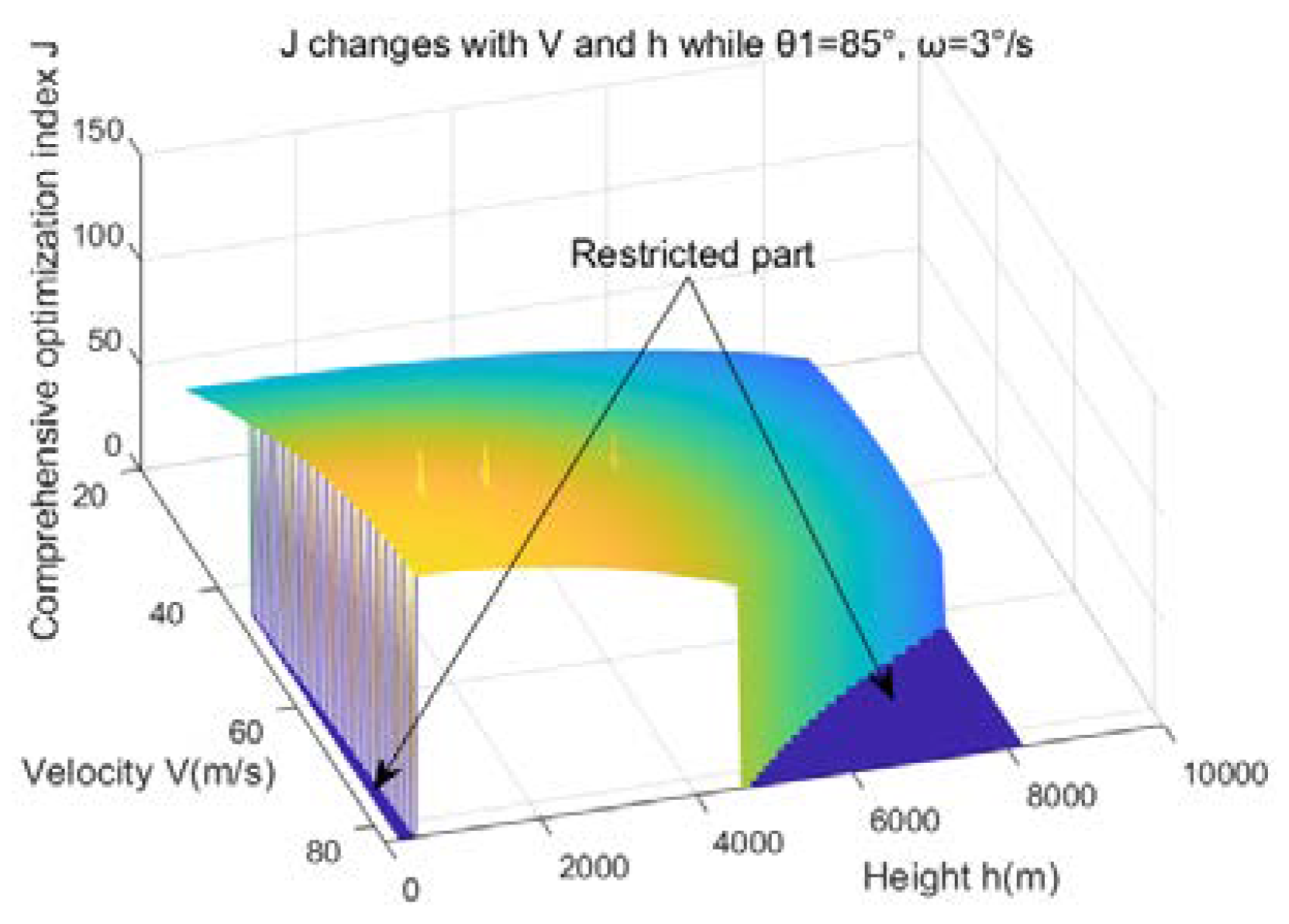
As shown in Figure 7, with search azimuth θ1 = 85° and scanning search angular velocity ω = 3°/s, J changed with V and h. It can be observed that the corresponding relationship was a curved surface. When V was large and h was high, there was a large restricted area and the parameters in this area did not meet the condition of complete coverage. When V was large and h was low, there was a small restricted area.
As shown in Figure 8, when V = 80 m/s and h = 3500 m, J changed with θ1 and ω. It can be seen that the corresponding relationship was also a curved surface. When ω was small and θ1 was large, there was a larger restricted area, and the parameters in this area did not satisfy the conditions of a complete coverage search.
When V and ω were unchanged, J changed with h and θ1, shown in Figure 9. When h and ω remained unchanged, the changes in J with V and θ1 are shown in Figure 10. In both cases, it can be seen that there were restricted areas and non-linear mutations.
From Figure 7, Figure 8, Figure 9 and Figure 10, it can be observed that there was no specific proportional relationship between J and a certain group of task parameters. Owing to many constraints, there was a non-linear mutation relationship, so it was difficult to solve such problems based on traditional analytical methods. Task parameter optimization was performed, based on IA, GWO, and VNS.

5.3. Task Planning Simulation Based on IA, GWO and VNS

The IA evolutionary algebra Era = 100 was set, and 10 rounds of task parameter planning were conducted. The results are presented in Table 2.
The maximum iterations of GWO were set as I max = 400 , and the running time of the GWO algorithm was similar to the 100 generations evolution time of the IA. Similarly, we set the maximum number of iterations of the VNS to I max = 500 . Tenrounds of task parameter planning were conducted, based on the GWO and VNS algorithms. The results are presented in Table 3 and Table 4, respectively.
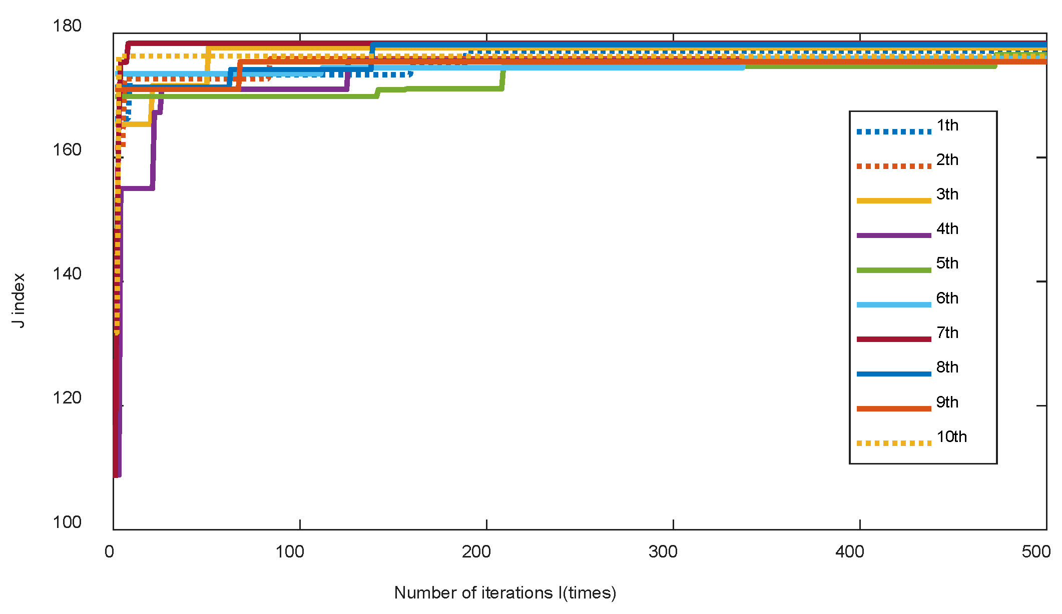
The change curves of fitness of 10 rounds of IA optimization are shown in Figure 11, the change curves of fitness of 10 rounds of GWO optimization are shown in Figure 12 and the curves of VNS are shown in Figure 13.
It can be seen from the simulation results that IA, GWO, and VNS obtained excellent task parameter sets, had high search efficiencies and comprehensive indices, and met the no-interval missing scan and speed-to-height ratio constraints. However, there were some differences in the results. Next, the differences in the parameter planning results of the three algorithms were compared and analyzed.
As shown in Figure 14, the optimal J index, average J index, and average time cost of the three algorithms were compared.
As shown in Figure 14, the planning results obtained by the three algorithms exhibited little difference in index J. However, in comparison, the results obtained based on IA were slightly better than those of the other two algorithms in terms of J. The optimal J index in the 10 rounds based on IA was 183.84, and the optimal J index in regard to GWO and VNS were 182.07 and 178.37, respectively. From the average J ¯ , the average J ¯ based on IA was 179.19, the average J ¯ based on GWO was 179.11, which was almost the same as that for IA, and the average J ¯ based on VNS was 176.72, which was significantly worse than those for IA and GWO. This showed that IA had a higher convergence accuracy when solving such problems, GWO was second, and VNS convergence accuracy was the lowest.
The J index change curves are shown in order to compare the convergence speeds of the three algorithms, and are given in Figure 15. At the same time, to make the image easy to observe and not too crowded, only the J index change curve of the optimal round of each algorithm was selected. The selected results were as follows: 1th round of IA, 1th round of GWO and 7th round of VNS. In addition, because IA had 100 evolution times, GWO 400 cycles, and VNS 500 cycles, the quantities of data are different, so the curves of IA and GWO are “stretched” to facilitate comparison.
As can be seen from Figure 16, in IA, the fitness of the optimal solution increased steadily, the change curve was relatively gentle, and there was “step” improvement during the operation, which indicated that the IA jumped out of the local optimal and converged in a position of relatively high precision. At the early stage of GWO, the fitness of the optimal solution ( α -wolf) increased rapidly, surpassing that of IA. In the subsequent process, the phenomenon of “step” improvement was constantly produced, which indicated that the GWO constantly jumped out of the local solution and converged to a relatively optimal position (slightly worse than IA). At the early stage of VNS, the fitness of the optimal solution increased the fastest, surpassing that of the IA and GWO algorithms. However, the optimization process then stagnated. This showed that VNS had the best optimization efficiency in the early stage, but the global optimization ability was relatively weak, and it was suitable for questions with high real-time requirements.
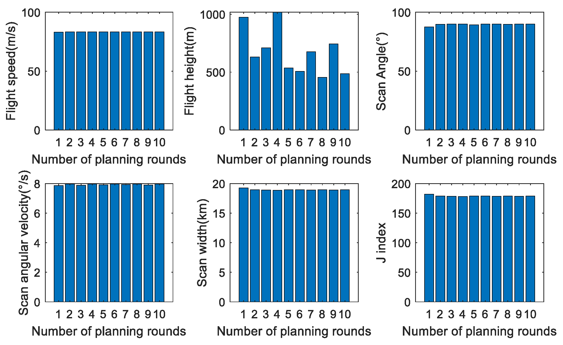
The optimization results were further analyzed. To facilitate the observation, the ten groups of planning results obtained by the three algorithms are presented in the form of bar charts in Figure 15, Figure 17 and Figure 18. It can be seen from the bar chart comparisons that the results obtained by the three algorithms tended to be consistent in each round for speed V and sector scanning Angle θ . In terms of flight height h , the results based on VNS were the most different, followed by GWO and IA. However, even the planning results of IA showed the largest difference in flight altitude h compared to other mission parameters, such as flight speed V . With respect to sector scanning angular velocity ω , the difference in planning results based on GWO was the smallest, and the difference between IA and VNS was relatively large. Overall, IA had the most stable planning results, followed by GWO and VNS.
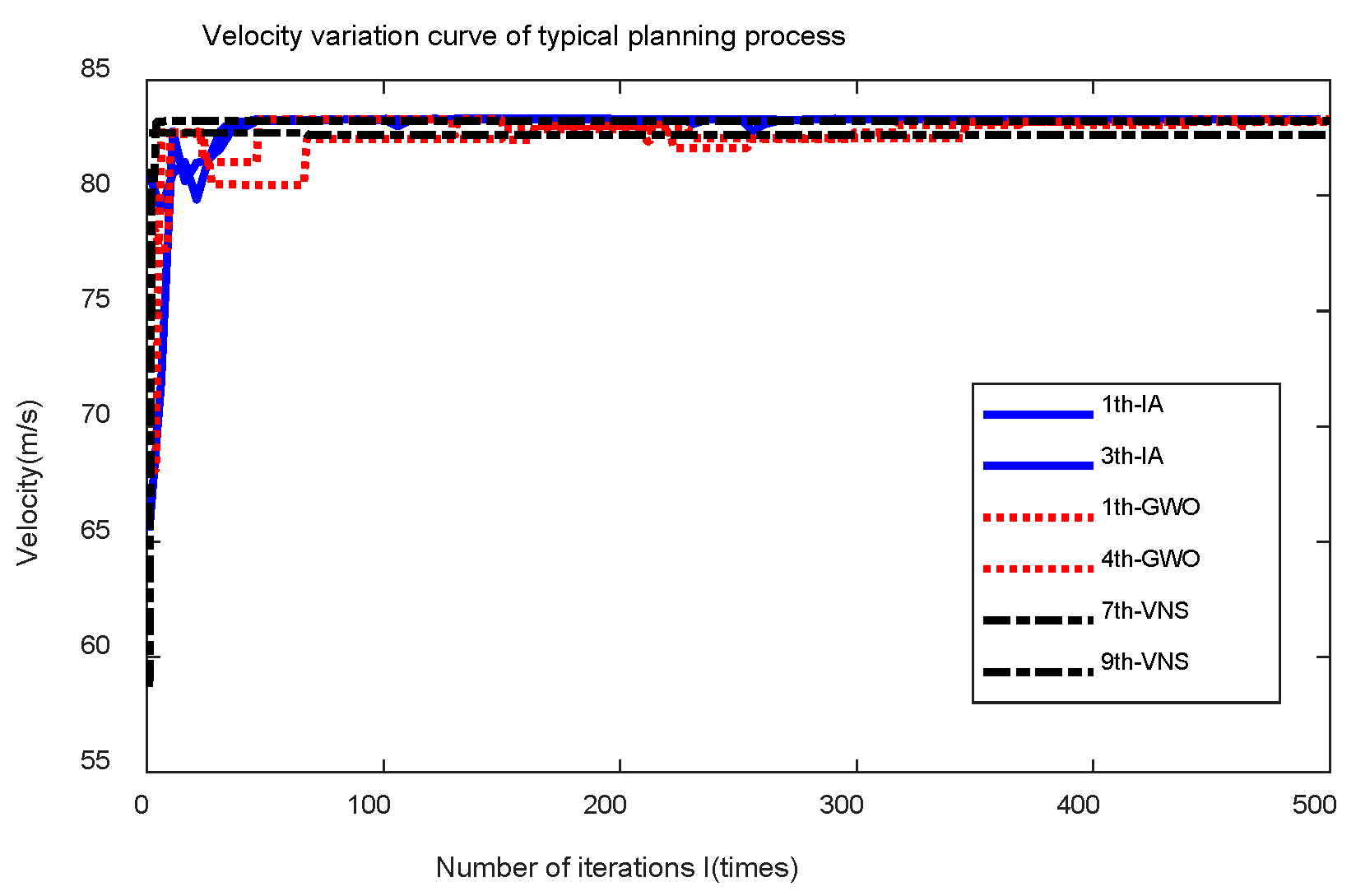
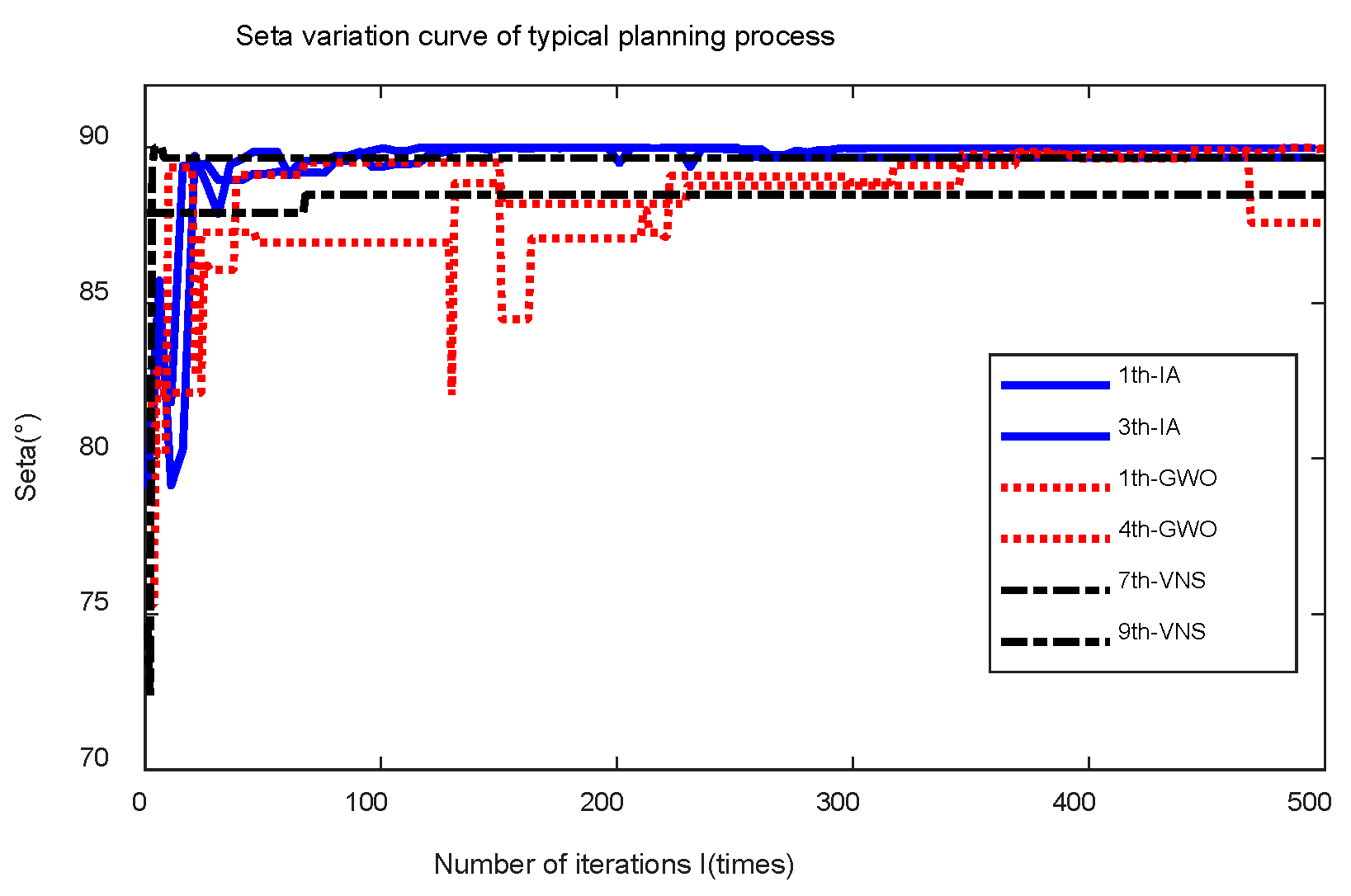
Furthermore, the changing process of the task parameters under a typical optimization process was compared. Similarly, to make the image less crowded, only the change curves of typical processes were selected for observation and comparison. The selection principle was that the J index was the best or the J index was the closest to the average. The selection results of IA were as follows: the 1th round and the 3th round; GWO selection results were: the 1th round and the 4th round; VNS selection results were: the 7th round and the 9th round.
The speed change curves of the typical rounds are shown in Figure 19. It can be seen that among the three optimization algorithms, the overall trend of speed was increasing, which reflected the positive significance of increasing speed for improving J index. The optimization efficiency of VNS was the highest, followed by GWO, with IA the slowest. Both GWO and IA exhibited oscillations in the early stage of operation, which reflected the complexity of the problem.
The change curves of h, θ , and ω are shown in Figure 20, Figure 21 and Figure 22. It can be seen that the change trend of height h in all three algorithms was downward overall, and the change trends of θ and ω were both increasing.
However, the optimization processes of the different algorithms exhibited significant differences. Basically, the optimization processes of VNS were the fastest, and sub-optimal solutions soon found, as shown in “7th-VNS” and “9th-VNS” in Figure 19, Figure 20, Figure 21 and Figure 22, while the subsequent processes were basically stable and unchanged. The GWO optimization process was also fast; however, the subsequent optimization processes entered a state of oscillation, as shown in “1th-GWO” and “4th-GWO” in Figure 19, Figure 20, Figure 21 and Figure 22. In the IA process, the variation curves of the parameters were relatively stable and gentle. This difference reflected the algorithmic characteristics of the three methods.
The change curves of coverage width d1 are shown in Figure 23. As d1 was the main component of J and its weight was much greater than that of the other indices, the trend of d1 was basically consistent with J.

5.4. Comparison of Area Coverage under Different Parameter Sets

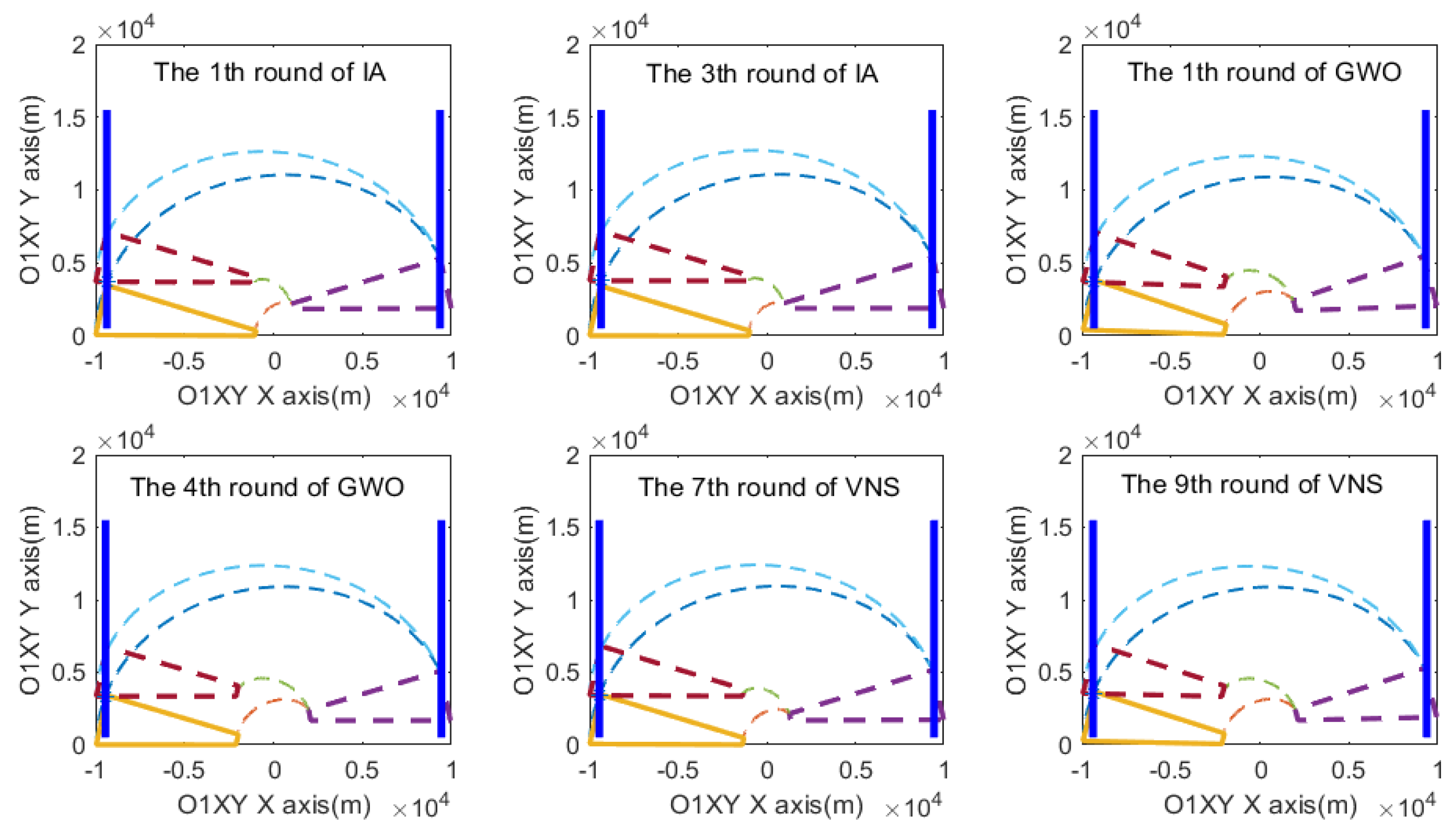
The scanning trajectory based on typical optimization results are shown in Figure 24. It can be seen that the optimized coverage widths were generally large and met all the constraints.
To demonstrate the advantages of the optimized task parameters, a coverage search was implemented based on different parameter sets. It was supposed that there was an area of 160 km × 80 km that had to be covered.
Test (a): Test (a) referred to the optimized task parameters using IA, and the 1th round planning results selected as an exampl.
Test (b): Test (b) referred to the optimized task parameters using GWO, and the 1th round planning results selected as an example.
Test (c): Test (c) referred to the optimized task parameters using VNS, and the 7th round planning results selected as an example.
Test (d): Test (d) referred to the parameters selected by experience, and the 4th group of parameters in Table 1 was selected as an example.
Test (e): The other task parameters were the same as in test (d), but the coverage width was determined according to the traditional method d 1 = 2 R 1 sin θ 1 , and the interval missing was not considered.
A common boustrophedon coverage method was adopted for the search track. The turning process, wherein the UAV completed a line scan and turned around, is shown in Figure 25. Assuming that the turning overload of the aircraft was 30 m/s2, the starting position of each scanning line (e.g., pturn) was 5 km from the edge of the area to be searched.
The coverage results of the area are shown in Figure 26a–e. Defining the miss ratio P m i s s e d = S m i s s e d / S a l l , S m i s s e d as the area missed in the coverage search, and S a l l as the total area. The time consumption and P m i s s e d of the five tests were calculated, and the results are presented in Table 5.
Compared with Test (e), the simulation results of Tests (a)–(c) showed that the coverage width model could achieve complete coverage of the target area without missing data. However, if the task parameters were simply determined by the traditional method, without considering miss scanning, the miss ratio P m i s s e d could be as high as 13.96% (Test (e)) indicated that the model and algorithm in this study are effective and necessary.
By comparing the results of Tests (a) and (d), it can be seen that both sets ensured no missed coverage. However, the empirical parameters cost 19,328 s to complete coverage, while the planned parameters had a shorter time consumption of 10,742 s, which was only 55.58% of the time cost of Test (d). Tests (b) and (c) were similar to test (a) and they were also significantly better than test (d). Therefore, the planned parameters had better coverage efficiency, and the algorithm designed in this study is effective and feasible.
By comparing the results of tests (a), (b), and (c), it was observed that the task parameters planned, based on IA, GWO, and VNS, could achieve an efficient search process without missing areas. When covering the area set in this study, there were no significant differences among the three sets of planning parameters. For example, the task completion times were 10,742 s (IA), 10,858 s (GWO), and 10,761 s (VNS). The planning result of IA was only slightly superior in terms of completion speed, 116 s faster than GWO and 19 s faster than VNS. This may not result in a significant difference in an actual mission. Therefore, all three algorithms are feasible. For offline task planning, IA and GWO could be the appropriate choices for time-efficient online task planning, while VNS and GWO could be the appropriate choices for online and real-time task parameter planning.

6. Conclusions

Automated target search and rescue must ensure complete coverage of an area. In this study, we conducted an in-depth study on task parameter planning when UAVs use EO equipment to cover areas in the sector scanning mode.
A model for the complete coverage width under sector scanning mode was established, and a model with no interval missing constraint and speed-to-height ratio constraint was also established. The test results indicated that the models were effective and reliable.
Although task planning is a serious nonlinear problem, the algorithm designed, based on IA, GWO, and VNS, can effectively solve task planning problems. The coverage process, based on optimized parameters, meets all constraints, has a higher search efficiency, and does not miss areas. Although all three optimization methods are feasible, they exhibit some differences. In general, IA is more suitable for offline occasions, VNS is more suitable for online real-time planning, and GWO has characteristics between the two.
The coverage task planning algorithm in this study can not only realize no-omission coverage but also consider the problem of target recognition, which provides technical support for fully automated target search and rescue.

Author Contributions

This article was jointly produced by all the authors. X.J. and M.H. identified the problem and suggested an idea. X.J. and M.H. designed the research methodology and W.L. provided valuable advice. X.J. and C.C. established a coverage-width model. Z.F. and C.C. reviewed the literature. X.J., M.H. and M.W. conducted the test experiments. X.J. and C.C. edited the manuscript. All authors have read and agreed to the published version of the manuscript.

Funding

This work was partially supported by the Science and Technology Planning Project of the Education Department of Jilin Province, China (Grant Number: JJKH20170966KJ).

Institutional Review Board Statement

Not applicable.

Informed Consent Statement

Not applicable.

Data Availability Statement

The data presented in this study are available in paper “Task Parameter Planning Algorithm for UAV Area Complete Coverage in EO Sector Scanning Mode”.

Conflicts of Interest

The authors declare no conflict of interest.

References

  1. Thibbotuwawa, A.; Bocewicz, G.; Nielsen, P.; Banaszak, Z. Unmanned Aerial Vehicle Routing Problems: A Literature Review. Appl. Sci. 2020, 10, 4504. [Google Scholar] [CrossRef]
  2. Al-Kaff, A.; Gómez-Silva, M.J.; Moreno, F.M.; de la Escalera, A.; Armingol, J.M. An Appearance-Based Tracking Algorithm for Aerial Search and Rescue Purposes. Sensors 2019, 19, 652. [Google Scholar] [CrossRef] [PubMed] [Green Version]
  3. Erdos, D.; Erdos, A.; Watkins, S.E. An experimental UAV system for search and rescue challenge. IEEE Aerosp. Electron. Syst. Mag. 2013, 28, 32–37. [Google Scholar] [CrossRef]
  4. Acar, E.U.; Choset, H.; Ji Yeong, L. Sensor-based coverage with extended range detectors. IEEE Trans. Robot. 2006, 22, 189–198. [Google Scholar] [CrossRef]
  5. Tan, L.Z.; Tan, P.; Wang, B. Computing Method of Aerial Searching’s Sweep Width at Sea. Ship Electron. Eng. 2019, 39, 146–150. [Google Scholar] [CrossRef]
  6. Yu, X.; Li, C.; Zhou, J. A constrained differential evolution algorithm to solve UAV path planning in disaster scenarios. Knowl.-Based Syst. 2020, 204, 106209. [Google Scholar] [CrossRef]
  7. Silvagni, M.; Tonoli, A.; Zenerino, E.; Chiaberge, M. Multipurpose UAV for search and rescue operations in mountain avalanche events. Geomat. Nat. Hazards Risk 2017, 8, 18–33. [Google Scholar] [CrossRef] [Green Version]
  8. Wang, Z.; Liu, L.; Long, T.; Wen, Y. Multi-UAV reconnaissance task allocation for heterogeneous targets using an opposition-based genetic algorithm with double-chromosome encoding. Chin. J. Aeronaut. 2018, 31, 339–350. [Google Scholar] [CrossRef]
  9. Chen, Z.; Yafei, L.U.; Hou, Z.; Wang, J. UAV’s Coverage Search Planning Algorithm Based on Action Combinations. J. Shanghai Jiao Tong Univ. 2019, 24, 48–57. [Google Scholar] [CrossRef]
  10. Long, D.; Rehm, P.J.; Ferguson, S. Benefits and challenges of using unmanned aerial systems in the monitoring of electrical distribution systems. Electr. J. 2018, 31, 26–32. [Google Scholar] [CrossRef]
  11. Maes, W.H.; Steppe, K. Perspectives for Remote Sensing with Unmanned Aerial Vehicles in Precision Agriculture. Trends Plant Sci. 2019, 24, 152–164. [Google Scholar] [CrossRef] [PubMed]
  12. Radoglou-Grammatikis, P.; Sarigiannidis, P.; Lagkas, T.; Moscholios, I. A compilation of UAV applications for precision agriculture. Comput. Netw. 2020, 172, 107148. [Google Scholar] [CrossRef]
  13. Xu, A.; Viriyasuthee, C.; Rekleitis, I. Optimal complete terrain coverage using an Unmanned Aerial Vehicle. In Proceedings of the 2011 IEEE International Conference on Robotics and Automation, Shanghai, China, 9–13 May 2011. [Google Scholar]
  14. Choset, H. Coverage of Known Spaces: The Boustrophedon Cellular Decomposition. Auton. Robot. 2000, 9, 247–253. [Google Scholar] [CrossRef]
  15. Mannadiar, R.; Rekleitis, I. Optimal coverage of a known arbitrary environment. In Proceedings of the 2010 IEEE International Conference on Robotics and Automation, Anchorage, AK, USA, 3–7 May 2010. [Google Scholar]
  16. Choset, H. Coverage for robotics—A survey of recent results. Ann. Math. Artif. Intell. 2001, 31, 113–126. [Google Scholar] [CrossRef]
  17. Lumelsky, V.J.; Mukhopadhyay, S.; Sun, K. Dynamic path planning in sensor-based terrain acquisition. IEEE Trans. Robot. Autom. 1990, 6, 462–472. [Google Scholar] [CrossRef]
  18. Acar, E.U.; Choset, H.; Rizzi, A.A.; Atkar, P.N.; Hull, D. Morse Decompositions for Coverage Tasks. Int. J. Robot. Res. 2002, 21, 331–344. [Google Scholar] [CrossRef]
  19. Zelinsky, A.; Jarvis, R.A.; Byrne, J.; Yuta, S. Planning paths of complete coverage of an unstructured environment by a mobile robot. In Proceedings of the International Conference on Advanced Robotics, Tokyo, Japan, 6–7 July 1993; pp. 533–538. [Google Scholar]
  20. Yang, S.X.; Luo, C. A neural network approach to complete coverage path planning. IEEE Trans. Syst. Man Cybern. Part B (Cybern.) 2004, 34, 718–724. [Google Scholar] [CrossRef]
  21. Perez-Carabaza, S.; Besada-Portas, E.; Lopez-Orozco, J.A.; de la Cruz, J.M. Ant colony optimization for multi-UAV minimum time search in uncertain domains. Appl. Soft Comput. 2018, 62, 789–806. [Google Scholar] [CrossRef]
  22. Majeed, A.; Lee, S. A New Coverage Flight Path Planning Algorithm Based on Footprint Sweep Fitting for Unmanned Aerial Vehicle Navigation in Urban Environments. Appl. Sci. 2019, 9, 1470. [Google Scholar] [CrossRef] [Green Version]
  23. Zhang, X.; Duan, H. An improved constrained differential evolution algorithm for unmanned aerial vehicle global route planning. Appl. Soft Comput. 2015, 26, 270–284. [Google Scholar] [CrossRef]
  24. Qu, C.; Gai, W.; Zhong, M.; Zhang, J. A novel reinforcement learning based grey wolf optimizer algorithm for unmanned aerial vehicles (UAVs) path planning. Appl. Soft Comput. 2020, 89, 106099. [Google Scholar] [CrossRef]
  25. Wu, X.; Bai, W.; Xie, Y.; Sun, X.; Deng, C.; Cui, H. A hybrid algorithm of particle swarm optimization, metropolis criterion and RTS smoother for path planning of UAVs. Appl. Soft Comput. 2018, 73, 735–747. [Google Scholar] [CrossRef]
  26. De Alcantara Andrade, F.A.; Reinier Hovenburg, A.; Netto de Lima, L.; Dahlin Rodin, C.; Johansen, T.A.; Storvold, R.; Moraes Correia, C.A.; Barreto Haddad, D. Autonomous Unmanned Aerial Vehicles in Search and Rescue Missions Using Real-Time Cooperative Model Predictive Control. Sensors 2019, 19, 4067. [Google Scholar] [CrossRef] [PubMed] [Green Version]
  27. Rafifandi, R.; Asri, D.L.; Ekawati, E.; Budi, E.M. Leader–follower formation control of two quadrotor UAVs. SN Appl. Sci. 2019, 1, 539. [Google Scholar] [CrossRef] [Green Version]
  28. Qingbo, W.; Shaolei, Z.; Yan, S. Multi-UAVs cooperative coverage reconnaissance in complex area. Tactical Missile Technol. 2016, 21, 50–55. [Google Scholar] [CrossRef]
  29. Wang, Y.; Li, Y.; Yin, F.; Wang, W.; Sun, H.; Li, J.; Zhang, K. An intelligent UAV path planning optimization method for monitoring the risk of unattended offshore oil platforms. Process Saf. Environ. Prot. 2022, 160, 13–24. [Google Scholar] [CrossRef]
  30. De Castro, A.I.; Torres-Sánchez, J.; Peña, J.M.; Jiménez-Brenes, F.M.; Csillik, O.; López-Granados, F. An Automatic Random Forest-OBIA Algorithm for Early Weed Mapping between and within Crop Rows Using UAV Imagery. Remote Sens. 2018, 10, 285. [Google Scholar] [CrossRef] [Green Version]
  31. Avellar, G.S.C.; Pereira, G.A.S.; Pimenta, L.C.A.; Iscold, P. Multi-UAV Routing for Area Coverage and Remote Sensing with Minimum Time. Sensors 2015, 15, 27783–27803. [Google Scholar] [CrossRef] [Green Version]
  32. Di Franco, C.; Buttazzo, G. Coverage Path Planning for UAVs Photogrammetry with Energy and Resolution Constraints. J. Intell. Robot. Syst. 2016, 83, 445–462. [Google Scholar] [CrossRef]
  33. Pestana, J.; Sanchez-Lopez, J.L.; Campoy, P.; Saripalli, S. Vision based GPS-denied Object Tracking and following for unmanned aerial vehicles. In Proceedings of the 2013 IEEE International Symposium on Safety, Security, and Rescue Robotics (SSRR), Linköping, Sweden, 21–26 October 2013. [Google Scholar]
  34. Al-Kaff, A.; Martn, D.; Garca, F.; Escalera, A.d.l.; Armingol, J.M. Survey of computer vision algorithms and applications for unmanned aerial vehicles. Expert Syst. Appl. 2018, 92, 447–463. [Google Scholar] [CrossRef]
  35. Cheng, G.; Zhou, P.; Han, J. Learning Rotation-Invariant Convolutional Neural Networks for Object Detection in VHR Optical Remote Sensing Images. IEEE Trans. Geosci. Remote Sens. 2016, 54, 7405–7415. [Google Scholar] [CrossRef]
  36. Lygouras, E.; Santavas, N.; Taitzoglou, A.; Tarchanidis, K.; Mitropoulos, A.; Gasteratos, A. Unsupervised Human Detection with an Embedded Vision System on a Fully Autonomous UAV for Search and Rescue Operations. Sensors 2019, 19, 3542. [Google Scholar] [CrossRef] [PubMed] [Green Version]
  37. Sun, J.; Li, B.; Jiang, Y.; Wen, C.-y. A Camera-Based Target Detection and Positioning UAV System for Search and Rescue (SAR) Purposes. Sensors 2016, 16, 1778. [Google Scholar] [CrossRef] [PubMed] [Green Version]
  38. Greenlaw, R.; Hoover, H.J. CHAPTER 1—Introduction. In Fundamentals of the Theory of Computation: Principles and Practice; Greenlaw, R., Hoover, H.J., Eds.; Morgan Kaufmann: Oxford, UK, 1998; pp. 1–18. [Google Scholar]
  39. Mulvey, J.M.; Vanderbei, R.J.; Zenios, S.A. Robust Optimization of Large-Scale Systems. Oper. Res. 1995, 43, 264–281. [Google Scholar] [CrossRef] [Green Version]
  40. Fomin, F.V. Proceedings of the Graph-Theoretic Concepts in Computer Science: 32nd International Workshop, WG 2006, Bergen, Norway, 22–23 June 2006.
  41. Mirjalili, S.; Mirjalili, S.M.; Lewis, A. Grey Wolf Optimizer. Adv. Eng. Softw. 2014, 69, 46–61. [Google Scholar] [CrossRef] [Green Version]
  42. Seyyedabbasi, A.; Kiani, F.; Allahviranloo, T.; Fernandez-Gamiz, U.; Noeiaghdam, S. Optimal data transmission and pathfinding for WSN and decentralized IoT systems using I-GWO and Ex-GWO algorithms. Alex. Eng. J. 2023, 63, 339–357. [Google Scholar] [CrossRef]
  43. Zhang, X.; Ren, Y.; Zhen, G.; Shan, Y.; Chu, C. A color image contrast enhancement method based on improved PSO. PLoS ONE 2023, 18, e0274054. [Google Scholar] [CrossRef] [PubMed]
  44. Wang, J.; Ersoy, O.K.; He, M.; Wang, F. Multi-offspring genetic algorithm and its application to the traveling salesman problem. Appl. Soft Comput. 2016, 43, 415–423. [Google Scholar] [CrossRef]
  45. Shen, Y.; Gao, Y.; Yuan, M.; Sun, H.; Guo, Z. Multi-Objective Immune Optimization of Path Planning for Ship Welding Robot. Electronics 2023, 12, 2040. [Google Scholar] [CrossRef]
  46. Kong, M.; Zhou, J.; Pei, J.; Liu, X.; Pardalos, P.M. A modified variable neighborhood search algorithm for manufacturer selection and order acceptance in distributed virtual manufacturing network. Optim. Lett. 2022, 16, 117–135. [Google Scholar] [CrossRef]
  47. Razzaq, S.; Xydeas, C.; Mahmood, A.; Ahmed, S.; Ratyal, N.I.; Iqbal, J. Efficient optimization techniques for resource allocation in UAVs mission framework. PLoS ONE 2023, 18, e0283923. [Google Scholar] [CrossRef] [PubMed]
  48. Bensi, E.A.B.; Spijkerman, R.; Brown, P.A.; Knights, S.; Nellensteijn, D.R. Helicopter-Based Search and Rescue Operations in the Dutch Caribbean: A Retrospective Analysis. Wilderness Environ. Medicine 2023, 34, 31–37. [Google Scholar] [CrossRef] [PubMed]
  49. Arkin, V. A Problem of Optimum Distribution of Search Effort. Theory Probab. Its Appl. 1964, 9, 159–160. [Google Scholar] [CrossRef]
  50. Zhang, K.; Chen, M.; Xu, X.; Yen, G.G. Multi-objective evolution strategy for multimodal multi-objective optimization. Appl. Soft Comput. 2021, 101, 107004. [Google Scholar] [CrossRef]
  51. Yang, Y.; Liu, J.; Tan, S. A multi-objective evolutionary algorithm for steady-state constrained multi-objective optimization problems. Appl. Soft Comput. 2021, 101, 107042. [Google Scholar] [CrossRef]
  52. Du, W.; Zhong, W.; Tang, Y.; Du, W.; Jin, Y. High-Dimensional Robust Multi-Objective Optimization for Order Scheduling: A Decision Variable Classification Approach. IEEE Trans. Ind. Inform. 2019, 15, 293–304. [Google Scholar] [CrossRef] [Green Version]
Figure 1. Schematic diagram of the sector scanning mode of the UAV EO equipment.
Aerospace 10 00612 g001
Figure 2. Schematic diagram of static view field of the UAV EO equipment.
Aerospace 10 00612 g002
Figure 3. Sector scanning process in a cycle of UAV EO equipment.
Aerospace 10 00612 g003
Figure 4. Schematic diagram of the speed-to-height ratio solution at any point in the coverage area.
Aerospace 10 00612 g004
Figure 5. Schematic diagram of the interval missing area in sector scanning mode.
Aerospace 10 00612 g005
Figure 6. Simulation and comparison of coverage process and coverage area under 6 sets of empirical parameters.
Aerospace 10 00612 g006
Figure 7. When θ1 = 85° and ω = 3°/s, the change of J along with V and h.
Aerospace 10 00612 g007
Figure 8. When V = 80 m/s, h = 3500 m, the change of J along with θ1 and ω.
Aerospace 10 00612 g008
Figure 9. When V = 80 m/s, ω = 3°/s, the change of J along with h and θ1.
Aerospace 10 00612 g009
Figure 10. When ω = 3°/s, h = 3500 m, the change of J along with θ1 and V.
Aerospace 10 00612 g010
Figure 11. The change curves of fitness of 10 rounds of IA optimization.
Aerospace 10 00612 g011
Figure 12. The change curves of fitness of 10 rounds of GWO optimization.
Aerospace 10 00612 g012
Figure 13. The change curves of fitness of 10 rounds of VNS optimization.
Aerospace 10 00612 g013
Figure 14. Comparison of the optimal J index, the average J index and the average time cost of the three algorithms.
Aerospace 10 00612 g014
Figure 15. Bar chart comparison of IA 10 round planning results.
Aerospace 10 00612 g015
Figure 16. Comparison of the J index change curves of the optimal rounds.
Aerospace 10 00612 g016
Figure 17. Bar chart comparison of GWO 10 round planning results.
Aerospace 10 00612 g017
Figure 18. Bar chart comparison of VNS 10 round planning results.
Aerospace 10 00612 g018
Figure 19. Comparison of the speed change curves of typical rounds.
Aerospace 10 00612 g019
Figure 20. Comparison of the flight height h curves of typical rounds.
Aerospace 10 00612 g020
Figure 21. Comparison of the angle θ change curves of typical rounds.
Aerospace 10 00612 g021
Figure 22. Comparison of the angle velocity ω change curves of typical rounds.
Aerospace 10 00612 g022
Figure 23. The changing curves of d1 of these typical rounds.
Aerospace 10 00612 g023
Figure 24. The comparison of coverage width under six sets of optimized task parameters.
Aerospace 10 00612 g024
Figure 25. Schematic diagram of U-turn after completing a scanning line.
Aerospace 10 00612 g025
Figure 26. Area coverage tests based on different sets of parameters.
Aerospace 10 00612 g026
Table 1. Six sets of task parameters and their corresponding coverage width and coverage efficiency.
Serial
Number
V (m/s)h (m) θ 1 (°) ω (°/s) d 1 (m) η (m2/s)
(a)8035007525822.3465,784
(b)70250060311,968.2837,774
(c)60200080314,979.7898,782
(d)83300080414,161.51,175,406
(e)831500852.59877.3819,816
(f)835000852.57105.5589,757
Table 2. Ten rounds of planning results based on the IA.
Serial NumberV (m/s)h (m) θ 1 (°) ω (°/s) d 1 (m) η (m2/s) J T I A (s)
183.30432.8589.687.2619.361.61183.8447.66
283.33398.3389.997.2918.771.56178.0357.31
383.32418.9289.987.0718.711.56177.7251.14
483.33418.0689.997.2618.761.56177.9653.22
583.33409.0089.987.8518.951.58179.1260.77
683.33442.6590.007.5618.871.57178.6747.48
783.21400.9189.947.7018.971.58179.2354.05
883.29429.0789.998.0019.011.58179.4145.22
983.33396.6889.998.0019.011.58179.5244.14
1083.33407.8489.997.4818.831.57178.3742.70
Table 3. Ten rounds of planning results based on the GWO.
Serial
Number
V (m/s)h (m) θ 1 (°) ω (°/s) d 1 (m) η (m2/s) J T I A (s)
183.22974.9087.597.8619.271.60182.0758.06
283.32630.7289.837.9818.941.58178.8145.86
383.33709.0289.987.8818.901.58178.6553.97
483.331017.4589.977.9718.871.57178.2268.81
583.29535.7289.287.9218.961.58179.0246.38
683.32507.0090.007.9718.951.58178.9945.12
783.32675.9989.977.9318.921.58178.7244.57
883.33455.8289.847.9818.951.58178.9538.47
983.32744.3789.997.9018.901.58178.6261.12
1083.33487.3889.977.9818.951.58179.0237.62
Table 4. Ten rounds of planning results based on the VNS.
Serial
Number
V (m/s)h (m) θ 1 (°) ω (°/s) d 1 (m) η (m2/s) J T I A (s)
183.01575.3889.377.5018.771.56177.0742.07
283.311654.5489.357.9618.631.55175.9346.29
383.21400.8689.507.4818.791.56177.7138.82
482.64474.1589.037.2218.671.54175.6240.13
583.281437.2389.997.6118.661.55176.5837.40
683.23582.7687.297.7218.641.55175.9837.24
783.23589.8589.667.9218.901.57178.3742.71
883.20463.4989.997.5318.841.57178.1540.09
982.631041.8888.477.9118.741.55175.4137.88
1083.261331.9089.067.8018.671.55176.3541.46
Table 5. Comparison of main indices of three simulation tests.
Test (a)Test (b)Test (c)Test (d)Test (e)
Coverage width d1 (m)18,73118,64318,90411,96819,071
Number of scanning lines999149
Time to complete coverage (s)10,74210,85810,76119,32811,331
Miss ratio Pmissed0%0%0%0%13.96%
Disclaimer/Publisher’s Note: The statements, opinions and data contained in all publications are solely those of the individual author(s) and contributor(s) and not of MDPI and/or the editor(s). MDPI and/or the editor(s) disclaim responsibility for any injury to people or property resulting from any ideas, methods, instructions or products referred to in the content.

