Aerodynamic Modeling of a Flying Wing Featuring Ludwig Prandtl’s Bell Spanload

Abstract

This paper presents the aerodynamic modeling of a flying wing featuring Ludwig Prandtl’s bell spanload. The aerodynamic models are developed using a medium fidelity vortex-lattice method and using a Reynolds-Averaged Navier–Stokes computational fluid dynamics solution across a wide range of in-flow angle conditions. A methodology is developed to directly compare the spanwise force distributions from each method. Excellent agreement is seen in the prediction of spanwise inertial aerodynamic forces from each method, as well as in stability and control derivatives dominated by lift and moment contributions. The phenomenon of proverse yaw, caused by the twist distribution necessary to produce the bell spanload, is seen in the high and low-order analysis, with similar off-axis control power predicted.

1. Introduction

Drag minimization has been the primary focus of aircraft design over the last century, as power required to maintain level flight is directly related to the drag experienced at a given velocity. The consumption rate of onboard energy affects critical aircraft performance parameters, like endurance and range, which designers want to maximize to expand the capability of their aircraft. For a sub-sonic aircraft, opportunities for drag minimization are available through reduction of profile drag and induced drag contributions. Profile drag minimization is typically performed by aerodynamic shape optimization to reduce the effects of viscosity on the object in the flow at the specified operating condition. Profile drag is accounted for in the work described in this document, but it is not explicitly studied. The induced drag component scales with the square of the lift coefficient and is caused by trailing vortices and the associated downwash present in any flow-field after it is traversed by a three dimensional lifting surface. Conventional lifting-line theory, developed early in the history of aerodynamics by Prandtl [1], determined that minimum drag was found where the induced downwash was constant when traversing the wake trace in the farfield for a wing of a fixed span. Wings are commonly designed with a nearly elliptical lift distribution to approximate this constant downwash condition.

An alternative approach to minimizing induced drag was reported by Prandtl [2,3] in 1933. Instead of fixing the wing span to some value, Prandtl imposed a bending moment constraint to effectively design a wing capable of achieving a target magnitude of lift with an equivalent structural weight compared to the baseline elliptical spanload case. A bell-shaped spanwise loading resulted in a highly twisted wing with a wider wingspan than the baseline elliptically loaded wing supporting the same lift force. This tactic of utilizing an aggressive twist distribution to create a centrally-loaded wing with a larger aspect ratio at an equivalent structural cost has been studied by other researchers throughout the last 75 years. In 1950, Robert T. Jones generated a minimum drag solution with a root bending moment constraint [4] that showed with a 15% increase in span. When an appropriately designed twist distribution is implemented, an approximately 15% reduction in induced drag is achievable when compared to an elliptical distribution generating the same lift. This concept has been revisited, such as with an attempt to generalize the bending moment constraint [5]. Additionally, further study by a team at Utah State came to a similar conclusion when predicting the ideal distribution for an aircraft in steady flight [6] and when considering weight distribution across the wing [7]. Recent work has also incorporated viscous effects into a scheme very similar to Jones’ work by accounting for airfoil profile drag along the span. An interesting example can be found in Ref. [8], where twist angles along the span are solved for directly under lift and bending moment constraints. With viscosity, a shape similar the bell spanload is found to be optimum. Wroblewski and Ansell presented another set of theoretical results and experimental validation in Ref. [9] pointing towards the drag benefits of the longer wing with a bell shaped spanloading even with a viscous flow.

The studies referenced above were focused on the spanload design for wings. Integration of such concepts to reduce induced drag on an aircraft are explored by Kroo in Ref. [10]. In addition to planform/twist choice, he examines the use of non-planar or multi-surface lift systems and the inclusion of wing-tip devices to interact with the concentrated vorticity at the tip. Individually, all of the options provide significant opportunity for induced drag reduction. However, each concept has implications on practical considerations such as available fuel volume, structural weight, and Reynolds number effects which impact an aircraft’s overall mission. In some cases, the potential vortex drag advantages are overwhelmed by practical considerations and deemed inconsequential due to the relative magnitude of profile versus induced drag at cruise conditions, as we saw in the study by Kelly [11] at Oklahoma State University.

Regardless of whether or not the spanload design target provided the bell spanload is worth capitalizing on for a particular design, this research considers a beneficial implication of using the bell spanload distribution, elucidated well by Ref. [12] and repeated by [13]. The aggressive twist distribution required to achieve the bell spanload alters the projection of forces attributed to induced drag near the wingtip. The twist is of such significance that, local to the wingtip, the resultant inviscid aerodynamic force vector is tilted forward by upwash relative to the aircraft’s velocity vector, rather than aft. The total spanwise inviscid aerodynamic drag remains anti-parallel to aircraft velocity, with most sections of the wing experiencing downwash. Locating anti-symmetrically deflecting control surfaces in the wingtip region of the upwash results in proverse rather than adverse yaw upon roll control actuation. The NASA Armstrong research team [12] identified the bell spanload as the lift distribution utilized in avian flight on the basis of observed separation distance in formation flight. It is an example from nature where the proverse yaw effect is beneficial due to the lack of a dedicated vertical flying surface to overcome adverse yaw in the establishment of a banked turn. The previous work additionally claims that an optimally low-drag flying wing configuration is conceivable, which omits a vertical flying surface. As such, a flying wing configuration is carried forward in this study to remain relevant to the published literature and serves as a sterile test case where yaw due to aileron deflection will stand out without influence from an empennage.

The main contribution of this paper is seen to be the prediction of the salient feature of the bell spanload, considered to be the proverse yaw, using variable fidelity methods. While a comparison of these and other methods in terms of fidelity has been shown in the past in general in References [14,15,16,17,18,19,20], limited resources are available for study of aircraft similar to this one, with some examples in References [21,22]. This manuscript aims to study the difference in predictions from the two methods utilized for this specific aerodynamic characteristic, described by the $C_{N_{{\delta }_a}}$ control derivative. To reinforce this assertion that the proverse yaw prediction is caused by the bell spanload twist distribution, a comparison case omitting the twist distribution is utilized, with this wing then analyzed using both prediction methodologies.

2. Materials and Methods

2.1. Defining the Outer-Mold Line

A necessary step in the analysis of an aircraft is the generation of a geometry that exhibits the feature to be studied. For the bell spanload, a complex twist distribution must be incorporated, using aerodynamic and/or geometric twist. While analysis methods have shown that there are ways to design the planform to exhibit a lift or twist distribution [23], similar research by NASA Armstrong [12] served as inspiration for the wing design that was chosen. Many of the geometric parameters were very similar to those of this project, with modifications to allow for easier manufacturing of the wing in the fabrication space available at Oklahoma State University, which was a forethought when considering an addition to the research that includes flight test verification. The airfoil distribution was adopted from Bowers’ wing. The reader is referred to Reference [12] which thoroughly documents the coordinates for the airfoils used at various spanwise stations along the wing. Additionally, the geometry utilized is shared with a targeted flight dynamics analysis conducted by the authors in Ref. [24], with some further geometric description given in that manuscript. Geometric parameters for the configuration in this paper have been tabulated in

Table 1. Geometric Parameter.

Parameter	Value
Aspect Ratio	$14.99$
Taper Ratio	$0.247$
Sweep at $\frac{c}{4}$	$15.7°$
Span	$10.2$ ft

.

The reference angle of attack for the aircraft body-axis system was chosen to occur when the airfoil at the centerline sees an angle of attack of 8.32 degrees. The reasoning for this, as opposed to the more standard convention of referencing the angle of attack at which the airfoil at the centerline sees a local angle of attack of zero degrees, is to set the aircraft zero degree angle of attack close to the $C_L$ condition where the twist distribution results in the bell spanload. It can be seen in later analysis that this condition is approximately one degree away from the design condition. After the reference condition was established, the entire twist distribution could be applied. The twist is nonlinear and was specified at twenty-one half span sections, designed to the distribution shown in Figure 1.

A large amount of the twist is contained in the inboard sections of the wing, leading to a larger amount of lift generation occurring in this area of the wing. This is a product of the root bending moment constraint enforced for this distribution, with a small moment arm for the areas that produce the most lift. Areas near the tip will see the largest moment arm to the center-line of the wing but will show much lower lift coefficient values. Using a fixed twist distribution, rather than one modifiable by flexibility or trailing edge surface deflection, results in the bell spanload only being exhibited at a single $C_L$, which is targeted by all analysis in this paper and mirrors the value used in a design case by a team out of NASA Armstrong that conducted similar research [12]. The wing geometry is further described by a leading-edge sweep angle of seventeen degrees and a dihedral angle of two and four tenths degrees. A heavy amount of sweep is typical for flying wings as it aids in stability characteristics [25], allowing for the neutral point of the aircraft to shift aft, leaving a larger margin for the center of gravity location. A model was then created in both analysis tools that would be later used for analysis. The CAD model that shows these design points can be seen in Figure 2.

Given that the bell spanload is only realized at one aircraft flight condition, an artifact of a fixed twist distribution, and seeing how lower induced drag may be realized with a plain untwisted wing (of the same span) approximating an elliptical load distribution, the most notable advantage of its use on a flying-wing aircraft design is the purported presence of proverse yaw under symmetric aileron application. With correct application, perhaps mimicking bird flight without a dedicated vertical flying surface, a designer may wish to incorporate this complicated outer-mold line. To test the proverse yaw assertion, a model with and without the bell spanload twist distribution was created to enable direct comparison and to directly see the effect of the twist distribution on the adverse/proverse yaw characteristic in the computational experiments. The taper ratio present in the untwisted model was expected to result in a nearly elliptical lift distribution at the design lift coefficient. The airfoils, sweep angle, dihedral angle, and chord lengths were all kept constant for this model. By using this model as a comparison case, any differences in the results can be isolated to the twist distribution. Both the twisted and untwisted models support trailing edge surface deflection to study the effect of aileron application.

2.2. Low-Order Analysis

The inviscid analysis consists of the use of the vortex-lattice code AVL [26]. Vortexlattice methods (VLM) provide rapid aerodynamic configuration analysis; but, due to their theoretical foundation in potential flow, are not capable of predicting viscous aerodynamic effects. The steps taken in the utilization of this code involved finding the design point of the geometry described in Section 2.1. A goal-seeking application in the code utilized was used to find the flight condition such that $C_L=0.6$. This design point was used for consistency between this wing and Bowers wing, upon which a large portion of the geometry was based. This point became the basis of the comparisons used in the Section 3 when proverse yaw characteristics are presented. Yaw due to aileron deflection is all due to the induced drag component unless modified to incorporate viscous drag. It is unknown if the propensity to develop proverse yaw is impacted if the physics to model viscosity are incorporated.

The discretization of the wing included forty-two span-wise sections with ten chord-wise sections for each span-wise section. This can be visualized within the AVL program in Figure 3.

2.3. Computational Fluid Dynamics

Additional flow physics are considered by making similar aerodynamic predictions using a computational fluid dynamics (CFD) code. For this work, Siemens Industries Digital Software Simcenter STAR-CCM+, version 2022.1 out of Munich, Germany was utilized. A major drawback to the use of CFD in the early stages of design is the time commitment required to produce results. Generating an appropriate grid and took on the order of weeks, with results taking several hours per in-flow condition even on a high-performance supercomputer located on the campus of Oklahoma State University. This is in contrast to the VLM, whose entire setup and testing was completed in less than a week, run solely on a personal computer. This is specified to show the drawback of using this method as a designer for initial stages of development, which oftentimes includes iteration of design parameters. Similar analysis of a different flying wing configuration has been previously conducted at Oklahoma State University, as documented in Ref. [27], whereby CFD solutions were used in a iterative design loop to arrive at a desired spanloading.

The mesh utilized for this research is a polyhedral base mesh with a set of prism layers encompassing the boundary layer of the aircraft. The computational domain included a large wake refinement—about ten wingspans past the aircraft—to resolve downstream flow features. A slight variance along the span was allowed, in the form of five span-wise volumetric refinements, so changes in cross-sectional geometry could be refined to the needs of each section, mainly due to changes in airfoil shape and chord length along the span. A small area along the trailing edge was further refined to model the stagnation point in that area. The mesh on the skin of the half-span is shown in Figure 4, and the mesh at the symmetry plane can be seen in Figure 5.

Figure 5 shows a cross-sectional view of the mesh utilized during analysis. Since the effects of the boundary layer have been shown to vary significantly in the direction normal to the surface but retain near constant parameters in the perpendicular direction, the mesh can be made much more efficient through the use of this style of cell. A different strategy is used to configure the sizing of these cells. The last prism layer, farthest from the surface, was sized such that the volume of this cell was no less than half that of the first polyhedral cell. The main consideration, however, of sizing a set of prism layers is the first layer—the layer closest to the surface. The concept of a wall y+ is used to related this first layer to the flow conditions.

$$y^{+}=\frac{u_{\ast }y}{\nu }$$

(1)

where the y is the distance to the closest wall, the value sought after in this equation. The $\nu$ is the local kinematic viscosity, and the $u_{\ast }$ is considered to be the friction velocity. The definition used for this term is shown below.

$$u_{\ast }=\sqrt{\frac{{\tau }_w}{\rho }}$$

(2)

where the ${\tau }_w$ is the wall shear stress and the $\rho$ is the local fluid density. The wall y+ was set to 1 for this analysis with the chosen fluid of velocity (35 ft/s). Equation (1) was then solved for the y value so an appropriate first layer thickness could be found when the y+ value is equal to one. A better view of the prism layers utilized is shown below in Figure 6.

The physics model chosen for this research was a Reynold’s-Averaged Navier–Stokes (RANS) k-$\omega$ model. A segregated flow solver was utilized due to the low speed, incompressible flow that was assumed for the test. Standard sea level atmospheric conditions were assumed for all parameters where applicable. Static aerodynamic forces were solved over a range of angles of attack and sideslip.

Additionally, modified models were run for the twisted and untwisted wing with elevon controls deflected for roll and pitch commands. The more important deflection for this research is the anti-symmetric aileron deflection case, with an angle of 5 degrees used for this test. The addition of control surfaces allows for the most important parameter in testing the proverse yaw prediction of this wing, the $C_{N_{{\delta }_a}}$ control derivative, computed by finding the slope of output yaw moment coefficient versus input aileron deflection. The sign and magnitude of this derivative is important in describing the ability of the aircraft to produce the proverse yaw, particularly when compared to the VLM results lacking many of the flow physics included in the CFD portion of the study.

2.4. Mesh Refinement Study

To ensure the predictions shown in Section 3 are independent of mesh parameters, a mesh refinement study was performed. The refinement studied the effect of cell count on output aerodynamic properties. A balance between cell count and solution convergence be found for the aircraft to accelerate computations.

Figure 7 shows the lift coefficient refinement at the design point with respect to the cell count. Initial conditions were kept constant throughout the different tests in an attempt to minimize variability within tests. As can be seen, there is very little change after about 45 million cells for both wings, making this the optimal cell count when also considering run-time. For perspective, the run-time for the 45 million cell test was approximately a third of the 85 million cell test, the highest count shown. This optimum cell count is further demonstrated by Figure 8, the pitching moment refinement. The same cell count is shown to be optimal for these tests, with initial conditions and center of gravity kept constant.

The refinements for the lateral-directional terms were tested at the design $\alpha$ for two different $\beta$ angles. This was completed for both the rolling and yawing moment coefficients, denoted as $C_l$ and $C_N$, respectively, with the two bounds to the $\beta$ sweep tested for refinement. The same mesh settings that produced about 45 million cells on the $\alpha$ sweep were used for each of the cases that were not refined, and this was used as the base mesh for the cases that were refined.

Figure 9 shows the refinement for the yawing moment at the bounding $\beta$ angles of the sweep conducted, chosen to be $-5\le \beta \le 5$. This refinement shows similar results to the pitching moment refinement, with minor variance over the entire refinement sweep. The rolling moment refinement, shown in Figure 10, shows more variance in the lower cell count tests. There is a large jump in the second group of tests completed, seen in both $\beta$ angles. However, this value then decreases back to a convergence value. For both the $C_N$ and $C_l$, the convergence value happens at a slightly higher mesh value than the clean configuration, about 55 million. This mesh size was carried forward in the analysis.

2.5. Comparing the Low-Order and CFD Results

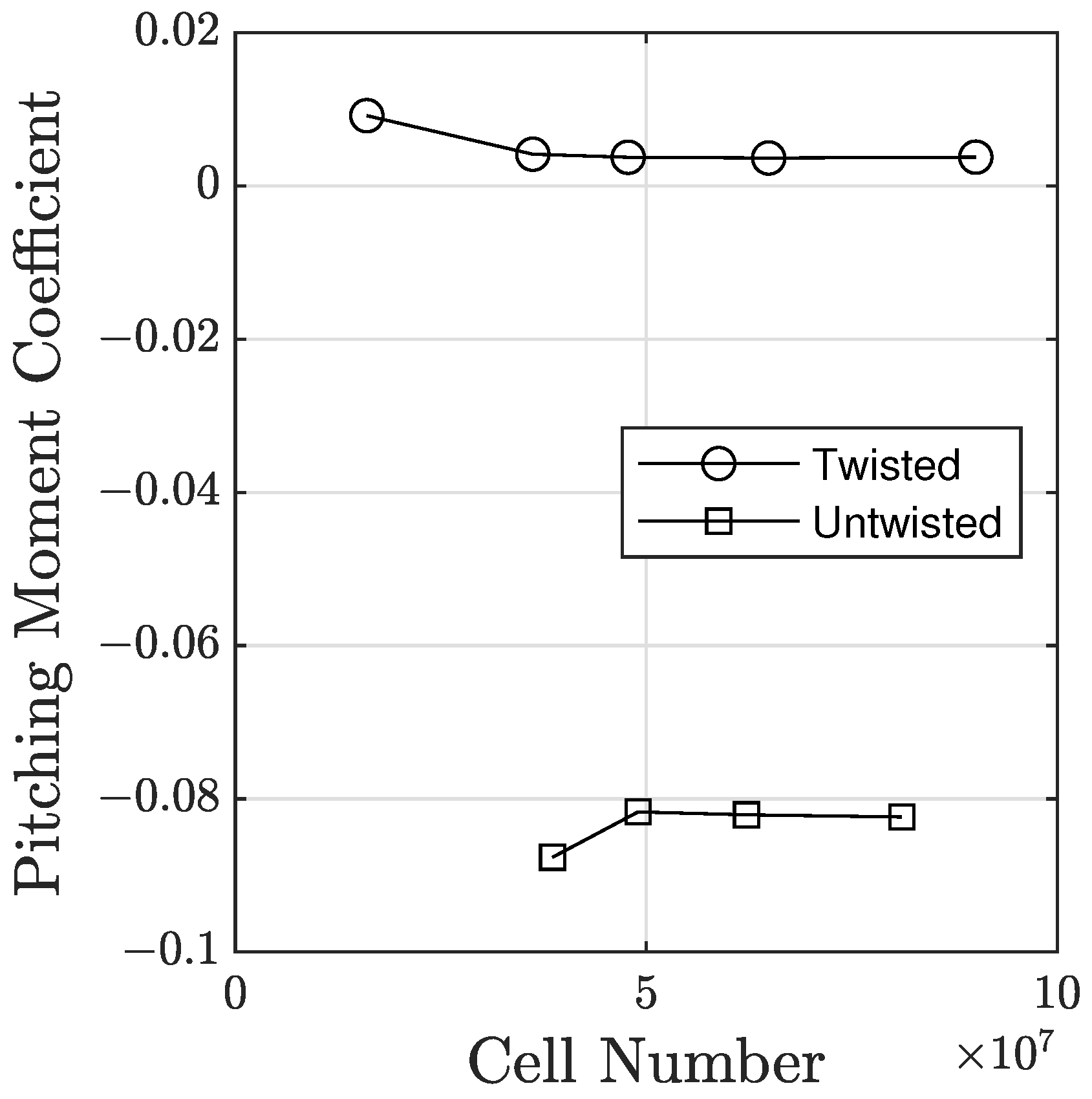
A contribution of this paper is the comparison of aerodynamic forces and the spanwise distribution of the forces from medium-fidelity vortex-lattice methods and a high-fidelity computational fluid dynamics solver. An overview of the outputs of each analysis method are provided below, followed by the methodology and sample results for comparing the medium- and high-fidelity approaches.

2.5.1. Span Load Comparison between VLM and CFD

The vortex-lattice method is a medium-fidelity approach for evaluating the aerodynamics of 3D wings subject to the limitations of potential flow. The formulation for this methodology is left to Ref. [28]. Knowledge of the circulation distribution across the span, an output of the formulated analysis, allows for computation of several aerodynamics quantities of interest to a designer seeking to match a given spanload. Applying the Kutta–Joukowski theorem gives the spanwise lift distribution:

$$L^{\prime }\left(y\right)=\frac{dL\left(y\right)}{dy}=\rho V_{\infty }\mathsf{\Gamma }\left(y\right)$$

(3)

Note that the $L^{\prime }$ distribution is the same shape as the $\mathsf{\Gamma }$ distribution since, for a given flow solution, the density and inflow velocity are constant in low-speed sub-sonic flow.

The total lift force developed by the wing is also of interest. This is found by summing the incremental lift contributions, $dL$, from each spanwise segment $dy$, which is written as

$$dL\left(y\right)=\rho V_{\infty }\mathsf{\Gamma }\left(y\right)dy$$

(4)

The local lift coefficient is often of interest to determine the local operating point of different segments of a wing to look at margin remaining until a local wing section would begin to stall (in purely 2-D flow), but is not directly related to the spanwise loading. From the definition of 2-D lift coefficient in airfoil theory, the lift per unit span can also be written as

$$L^{\prime }\left(y\right)=\frac{1}{2}\rho {V_{\infty }}^{2}c\left(y\right)C_l\left(y\right)$$

(5)

Therefore, the local lift coefficient at spanwise location y can be written as

$$C_l\left(y\right)=\frac{2\mathsf{\Gamma }\left(y\right)}{c\left(y\right)V_{\infty }}=\frac{2}{c\left(y\right)V_{\infty }}\mathsf{\Gamma }\left(y\right)$$

(6)

Rearranging Equation (6), it is seen that the $c\left(y\right)C_l\left(y\right)$ distribution is simply a scaled version of the $\mathsf{\Gamma }$ distribution. Thus, many readily available outputs from a vortex-lattice method or similar are seen to be the same shape and are simply scaled versions of each other, as indicated in Equation (7).

$$\mathsf{\Gamma }\left(y\right)\stackrel{\mathrm{Same}\mathrm{Shape}}{\to }{L}^{\prime }\left(y\right)=\rho V_{\infty }\mathsf{\Gamma }\left(y\right)\stackrel{\mathrm{Same}\mathrm{Shape}}{\to }c\left(y\right)C_l\left(y\right)=\frac{2}{V_{\infty }}\mathsf{\Gamma }\left(y\right)$$

(7)

The lift distribution shape is useful in an aerodynamics problem as it fully determines the induced drag that will result from producing the required amount of lift with a given spanload. The lift distribution is also useful for determination of wing structural loading and the overall wing-root bending moment. Because the spanload distribution is designed using a combination of geometric and aerodynamic twist, it is critically important to remember that $L^{\prime }\left(y\right)$, $\mathsf{\Gamma }\left(y\right)$, $dL$, and $c\left(y\right)C_l\left(y\right)$ distributions will all be the same shape and simply scaled versions of one another but that the spanwise distribution of local $C_l$ will result in a different shape because the chord is not constant along the span.

Based on the discussion leading up to Equation (7), the CFD results can be compared to the $c\left(y\right)C_l\left(y\right)$ from the VLM after extracting a $dL$ distribution at spanwise locations from the computational domain. This is performed in post-processing by splitting the wing into a number of sections along the span. For each section, the force over the surface is summed up in the direction of lift, taken to be perpendicular to $V_{\infty }$. The $dL\left(y\right)$ distribution created using this method can then be compared directly to the VLM output. It is important, however, to note that the shape is the only characteristic that can be compared between the two, not the specific values shown. Therefore, plots in Section 3 multiply the $dL\left(y\right)$ distribution by a scale factor to match the magnitude in the center of the wing.

In addition to the total lift, discussed above, the drag force is of interest to an aircraft designer. Since surface friction is not inherent in the formulation of a VLM, the drag prediction includes only contributions from lift-induced drag. Induced drag is predicted from a VLM after the $\mathsf{\Gamma }$ distribution is solved. Traditional VLM formulations calculate the induced drag in the Trefftz plane, theoretically located infinitely far behind the wing, using the equation below:

$$D_i=\frac{\rho }{2}\sum _{i=1}^n{\mathsf{\Gamma }}_i{V}_{n_t,i}d{s}_i$$

(8)

In Equation (8), $D_i$ is the total induced drag, $\rho$ is the density of the freestream flow, ${\mathsf{\Gamma }}_i$ is the bound circulation at spanwise wing station i, $V_{n_t,i}$ is the velocity normal to the wake in the Trefftz plane at spanwise station i, and $d{s}_i$ is the incremental distance along the span at section i. As the wake normal velocity in the Trefftz plane is simply the sum of all the velocity increments from each bound and trailing vortex in the lift system, the total induced drag is simply a function of the resultant $L^{\prime }\left(y\right)$ distribution. Similar to the $dL\left(y\right)$ distribution, the drag force acting on wing section $dy$ can extracted to study the spanwise distribution of drag and compare to VLM predictions.

2.5.2. Control Surface Deflections

A difference between how the two methods handle control surface deflections is also important to note. The VLM, which models the lifting surface as an infinitely thin surface following the mean camber line chordwise, simply tilts the normal vectors of panels which are part of the control surface being deflected.

CFD models a control deflection by changing the entire outer mold line of the geometry and each control deflection requires a new computational grid to be developed. The modified CAD representation of the wing with a trailing edge surface deflected is shown in Figure 11.

Although a physically realizable wing with a trailing edge surface will use a gap on the bottom surface to provide clearance for the aileron to deflect, a choice was made to not model this gap due to complexity of the mesh in this area. Instead, the area containing the aileron was adjusted to represent the deflection as a shift in the camber of the area containing the control surface. This is visualized in Figure 12, along with the slightly adjusted mesh in this area of the wing.

The differences between the mechanisms behind the aerodynamic predictions and the varying fidelity between VLM and CFD leads to an unknown variation in control power prediction. For instance, flow separation is possible and could lead to a misrepresentation by the VLM. Control surface deflections that are heavily dependent on viscous effects are known to be slightly overestimated by potential flow solvers [29,30]. The current research aims to inform designers how well the proverse yaw feature of the bell spanload can be predicted by medium fidelity methods compared to more involved approaches.

3. Results

Aerodynamic predictions for the twisted and untwisted wing were generated using the VLM and CFD. Initial results, in Section 3.1, considered static aerodynamic sweeps as $\alpha$ and $\beta$ were varied. Overall lift coefficient, lift distribution, drag, and aerodynamic moments were compared. After the static aerodynamic sweep data were generated, the effect of controls was studied in Section 3.2. The ability of VLM and CFD to predict proverse yaw and the degree to which the twist distribution contributes to this phenomenon are presented by direct comparison of the twisted and untwisted wing.

3.1. Static Aerodynamics with Fixed Controls

Static aerodynamic sweeps across a range of in-flow angles with controls fixed to the neutral position are presented in this section. Section 3.1.1 begins by showing the lift coefficient versus angle of attack for each wing from CFD and VLM. The resulting spanloads are also compared. Drag results are presented next in Section 3.1.2. Pitching moment coefficient results follow in Section 3.1.3 to include a comparison of the predicted neutral point from each aerodynamic analysis method. Lateral and directional static stability characteristics are documented in Section 3.1.4.

3.1.1. Lift Predictions

The analysis began with an angle of attack sweep such that the design point could be identified. Results for this sweep can be seen in Figure 13 for both wings using both analysis methods. The slopes of the lift polars provide useful insight into the response of the vehicle aerodynamics to change in flight condition and are shown for the twisted and untwisted wing in

Table 2. Lift Curve Slopes for Each Configuration and Method.

Configuration	Method	${\mathit{C}}_{{\mathit{L}}_{\mathit{\alpha }}}$ (Per Radian)
Twisted	CFD	0.07917
Twisted	VLM	0.091588
Untwisted	CFD	0.08446
Untwisted	VLM	0.09192

. The values for the VLM and linear portion of the CFD curves are close, even when comparing the twisted to untwisted wing, as the lift curve slope is primarily driven by planform, not the twist distribution.

The most immediate difference in Figure 13 is a reminder of the consequence of utilizing the VLM as a primary design tool. Since this method does not support stall effects, the lift curve continues to increase linearly, long past the point where stall is predicted by the CFD. Coupled with this is a small gap present between the methods’ curves for both wings. Along portions of the twisted and the entirety of the tested range of the untwisted wing, the CFD predicts a slightly higher lift coefficient at each angle of attack with a very similar slope. After stall occurs for the twisted wing, the VLM switched from under-predicting the lift coefficient to vastly overestimating it.

When an angle of attack that produced a value close to the design condition of $C_L=$ 0.6, the spanwise lift distributions could then be plotted and compared. The distribution of the wing that is expected to exhibit the bell spanload can also be validated in shape by comparison to the theoretical curve. The equation for this distribution, Equation (9), is pulled from Prandtl’s 1933 paper [3].

$$L^{\prime }(y)=L_{y=0}^{\prime }{(1-{(\frac{2y}{b})}^2)}^{\frac{3}{2}}$$

(9)

This equation, referred to as the bell spanload Equation in the plots below, is the baseline to which the lift distributions of both the CFD and VLM results will be compared. It must be noted that this distribution is only expected at the design condition. Any off-design points will not exhibit the design bell spanload distribution as the spanwise twist is fixed.

The lift distribution for the wing designed to exhibit the bell spanload is shown in Figure 14. The $c\left(y\right)C_l\left(y\right)$ distribution is pulled from the VLM results directly. The results of the CFD are represented as bars on this plot. Each bar represents an extracted incremental force value—in this case, in the direction perpendicular to the velocity vector—acting on a slice of the wing of non-dimensionalized width $dy$ and occupying a corresponding space on the span. A scaling factor is then applied to each value to compare the shape difference between the $c\left(y\right)C_l\left(y\right)$ distribution and the $dL\left(y\right)$ distribution.

As was shown by Equation (7), the shapes of the incremental lift distribution pulled from the CFD results, $dL$, and the $c\left(y\right)C_l\left(y\right)$ distribution from the VLM should match in shape. The CFD result show a near perfect match to the theory, confirming that this wing exhibits the bell spanload at the design point. Additionally, since the shapes are seen to match between methods, this same strategy of comparing these two parameters can be used going forward.

There is seen to be a slight difference between the lift distribution predicted by the VLM when compared to the shape of the baseline and CFD generated data. The shape predicted by the VLM exhibits a dip near the root, with a similar behavior to the plot of the twist distribution. After approximately twenty-five percent of the span in the inboard section, the shape begins to match well with the other methods, particularly the baseline.

For the wing omitting the twist distribution, Figure 15, the lift distribution is seen to be more elliptical. This is due to the lift generation being less localized in the root section of the wing, with both methods predicting similar behavior near the tip. A major effect of this is that the bending moment will be greater for this wing than one that produces the bell spanload, as well as impacts on induced drag, as pointed out in the next section.

3.1.2. Drag Predictions from VLM and CFD

The assumptions that led to the derivation of the bell spanload in Prandtl’s 1933 work are critically important to keep in mind when comparing the drag of a finite wing utilizing it to the drag of a more traditionally designed wing. The drag benefit of the bell spanload are only realized if the designer can accept a larger aspect ratio for the given wing area and manufacture the more complicated geometry. The investigation in this research aimed to determine the ability to predict the proverse yaw feature inherent due to the aggressive washout present with the Bell shaped lift distribution; thus, no span modifications between the twisted and untwisted wings were considered. Rather, they were the same span and held the same planform area.

Given two wings with the same span, minimum induced drag is found using Prandtl’s 1920 derivation, where span was held constant. The well known result from this work showed that minimum induced drag was found when downwash in the farfield is held nearly constant across the span, a condition that is met for a purely elliptical lift distribution (for a planar wing). The results in Figure 16 follow the expectations of Prandtl’s earlier theory. The drag coefficient is larger across the entire angle of attack range for the twisted wing, featuring the bell spanload, compared to the untwisted wing. As the twist distribution was not applied with an increase in aspect ratio, this result is expected. The other comparison to draw from comes from examining the drag predicted by the VLM versus the drag from the CFD. The VLM drag only considers induced drag following inviscid aerodynamic theory. When fluid viscosity is modeled, as in the RANS CFD results, a higher magnitude of drag is present. The drag from the twisted wing remains higher than that of the untwisted wing in the CFD results across the range of inflow angles studied.

3.1.3. Aerodynamic Center and Pitching Moment Predictions

Aerodynamic moment couples need to be reported about a defined location, in order to be transferable to other locations on the geometry. Commonly, moments are reported about the aircraft center of gravity (CG) since this is the location an object rotates about. The results in this section are reported about the CG, positioned to achieve an approximately 10 percent static margin for the twisted and untwisted wing. Static margin dictates longitudinal static stability of the aircraft and is represented mathematically by Equation (10). Essentially, static margin is a measure of the distance between the center of gravity, $x_{cg}$, and neutral point, $x_{NP}$, as a percentage of the average chord, $\overline{c}$.

$$\sigma =\frac{x_{NP}-x_{cg}}{\overline{c}}$$

(10)

Both $x_{cg}$ and $x_{NP}$ are measured from the nose of the aircraft—in this case, the leading edge of the airfoil at the centerline. To retain longitudinal static stability, this value should be a positive number, meaning the neutral point is aft of the center of gravity. When this constraint is upheld, the slope of the plot when pitching moment is plotted over a range of lift values will be negative, shown in Figure 17.

Since the slope of Figure 17 is negative, the aircraft is statically stable about the longitudinal axis. The placement of the center of gravity is determined using the relationship between this location and the point where the pitching moment is about zero at the design condition. This will trim the aircraft at a point, with the $C_L=0.6$ design condition used as the goal of this zero pitching moment. The VLM was then used to quickly iterate to find this point. The pitching moment from the CFD was then calculated using the new center of gravity, determined to be 8.79 inches aft of the reference point.

An additional insight to be gathered from this plot is the closeness of the two predictions. When the same center of gravity is utilized, the plots match closely between methods. For both wings, the slope of the CFD results matches the VLM almost exactly. This shows that, since the center of gravity is the same between methods, the aerodynamic center prediction is also about same. The aerodynamic center location can be calculated to be about 10.1 inches aft of the leading edge of the center-line cross-section. This correlates with a static margin of 14.6 percent of the mean chord.

Finally, it is noted that the untwisted version of the wing geometry studied does not represent a useful aircraft, since it is not possible to trim at a positive $C_L$. This, of course, is due to the lack of a twist distribution to move the centroid of the aerodynamic loads forward, as is performed for the case exhibiting the bell spanload. The static aerodynamic results, however, remain valid and will be used to assess the ability to predict proverse/adverse yaw later in this paper.

3.1.4. Rolling Moment and Yawing Moment Due to Sideslip

The rolling moment due to sideslip governs static lateral stability for an aircraft configuration. Similarly, the directional static stability is determined by the yaw moment response to sidelsip. Each are studied in this section. The slopes of the rolling and yawing moment coefficients across sideslip angles offset from trim are catalogued below in

Table 3. Beta-Dependent Stability Derivatives Per Radian.

Configuration	Method	${\mathit{C}}_{{\mathit{l}}_{\mathit{\beta }}}$ (Per Radian)	${\mathit{C}}_{{\mathit{N}}_{\mathit{\beta }}}$ (Per Radian)
$Twisted$	$CFD$	−0.0176	0.000709
$Twisted$	$VLM$	−0.0615	0.000760
$Untwisted$	$CFD$	−0.0132	0.00143
$Untwisted$	$VLM$	−0.0426	0.00697

from the VLM and CFD analysis.

Looking first at the lateral stability parameter, $C_{l_{\beta }}$, it is observed that the twisted wing predicts a slightly higher value compared to the untwisted wing. The values between the VLM and CFD methods are shown to exhibit some differences, although it is most important to note that they are consistent in sign and of the same order of magnitude. The consistent negative slopes for $C_{l_{\beta }}$ indicate lateral static stability for all cases even though the value reported by the CFD is shown to be about a third of the VLM prediction.

The values predicted by both methods show a lack of directional static stability, well below the values recommended by well known design guidelines, such as that by Raymer [31]. This is an artifact of the configuration lacking a vertical tail, which most aircraft take advantage of to support this parameter. Due to the lack of this feature, even with the proverse yaw predicted, there may still be issues related to the directional stability of the aircraft.

To compare the predictions between methods, there is more agreement than with the $C_{l_{\beta }}$. The $C_{N_{\beta }}$ values of the twisted wing match almost exactly, with a small difference present. The untwisted wing shows more variance, with the CFD prediction being about a third of the VLM prediction.

3.2. Control Effects

This section reports the control derivatives for the elevon effects on the aircraft. Three effects are examined, with the first being the pitch control in Section 3.2.1, where each surface deflects symmetrically either trailing edge up or down. Next, the control powers under anti-symmetric elevon deflection are considered, starting with roll control power in Section 3.2.2. The yaw moment associated with aileron deflection is examined in Section 3.2.3, where the proverse yaw feature of the bell spanload is highlighted by comparing the differences between the twisted and untwisted wing.

3.2.1. Elevator Control Power

The elevator control power is described as the change in pitching moment due to a change in elevator deflection angle. For this configuration, the elevator and aileron deflections are conducted with the same surfaces, with an elevator deflection simulated using a symmetric deflection of the ailerons. A consistent trend is a slight overestimation by the VLM. Potential flow solvers have shown to over-estimate parameters that are heavily influenced by viscous effects [29,30], including elevator deflections. This is thought to account for the small difference between the two.

As is seen in

Table 4. Elevator Control Power per Degree of Deflection.

Configuration	Method	${\mathit{C}}_{{\mathit{M}}_{{\mathit{\delta }}_{\mathit{e}}}}$
$Twisted$	$CFD$	−0.0176
$Twisted$	$VLM$	−0.0615
$Untwisted$	$CFD$	−0.0132
$Untwisted$	$VLM$	−0.0426

, the values of the elevator control power are shown to be close for both wings for both methods. By looking at the lift distribution for these cases, Figure 18 and Figure 19, the magnitude of change caused by the elevator deflection is shown to be fairly consistent throughout each case. A similar difference in shape between methods can be seen near the root for this distribution as with the clean configuration.

The predictions made by both methods for both wings are shown to be relatively equivalent. This is an expected result, as the effect of the elevator deflection is primarily based on the geometry and location of the control surfaces, which is equal for all cases. As can be seen by Figure 18 and Figure 19, for both wings, the methods match well in terms of shape and relative magnitude of the deflection. The twisted case shows a perfect match in shape of the region close to the deflection, leading to the very similar control derivative results. For the untwisted wing, there is more variance in shape, consistent with the clean distribution, with the effect of the elevator shown to be nearly identical.

3.2.2. Aileron Control Power

The aileron control power was similarly quantified as a control derivative to show the difference between the two aerodynamic prediction approaches. Implementation simply required capturing the difference between tests with differing aileron deflection angles when the $C_L$ = 0.6 flight condition is considered.

Table 5. Aileron Control Power per Degree of Deflection.

Configuration	Method	${\mathit{C}}_{{\mathit{l}}_{{\mathit{\delta }}_{\mathit{a}}}}$
$Twisted$	$CFD$	−0.00124
$Twisted$	$VLM$	−0.00126
$Untwisted$	$CFD$	−0.000982
$Untwisted$	$VLM$	−0.00119

shows the values calculated for both wings using both methods. Small changes are observed both between methods and even between wings.

Figure 20 and Figure 21 offer some insight with the resulting lift distribution of the maximum deflection case tested.

When the lift distribution is compared between method for each wing, there is little difference in the area that includes the control surfaces. Figure 20 specifically shows the twisted wing, with no visual difference between the $L^{\prime }\left(y\right)$ distribution of the CFD and $c{C}_l\left(y\right)$ distribution of the VLM. The untwisted wing, shown in Figure 21, presents a slight difference, although the shape of the two plots stays constant.

3.2.3. Yaw Due to Aileron Deflection

The derivative most pertinent to this research focus is $C_{N_{{\delta }_a}}$, the yawing moment sensitivity to a change in aileron deflection. Prediction results for this quantity are displayed in

Table 6. $C_{N_{{\delta }_a}}$ per Degree of Deflection.

Configuration	Method	${\mathit{C}}_{{\mathit{N}}_{{\mathit{\delta }}_{\mathit{a}}}}$
$Twisted$	$CFD$	−0.00000268
$Twisted$	$VLM$	−0.00000600
$Untwisted$	$CFD$	0.0000686
$Untwisted$	$VLM$	0.000062

. This derivative will describe whether the system exhibits the proverse yaw predicted by the VLM or if viscous effects change the behavior. An important factor for the yawing moment is the drag distribution at the condition of interest. In this case, due to the symmetric nature of the wing, this would be when the ailerons are deflected. A convenient comparison case is the drag distribution for the same deflection case, and the same lift coefficient, on the untwisted wing.

Although the Bowers paper [12] does not present the same aerodynamic analysis, there is an estimation given of the principle result, the $C_{N_{{\delta }_a}}$, in that paper. That analysis presents the comparison between the flight test estimations and a vortex-lattice method ran for their geometry. While this is the only aerodynamic prediction presented within that paper for this result, a comparison can be drawn, with a percent difference gathered of 15.2%. However, with the results staying of similar magnitude, there is seen to be some validation of the results gathered in this analysis.

The contributions of drag can be separated to show the composition and shape of both the pressure and shear drag, seen in Figure 22 and Figure 23. For both cases, the pressure drag is the dominant cause of the shape of the plot. The shear forces in this drag direction are seen to be much more constant than the pressure drag, with a linear increase to the root, where the peak is reached. The distribution for the twisted wing, shown in Figure 22, shows that the total distribution is much lower near the wing tip for the side of the wing in the positive direction. For orientation, the deflection takes place on the outboard 14 percent of the half span described by positive x-axis values. On the twisted wing, the pressure drag on this deflection side is seen to sit close to the x-axis, even predicting a negative pressure drag component in some areas of the deflection. This drag behavior starts at about 75 percent of the half span on either side. In the areas of the aileron itself, a slight jump in pressure drag corresponds to a pressure drag prediction of about zero. On the other side, the pressure drag falls just below the x-axis at about the same location before quickly increasing to a much higher magnitude.

The lower total drag on the right side of the plot causes a yawing moment to the left side of the plot. The orientation of the plot lends itself to a proverse prediction to be made by the CFD, albeit lower than the VLM prediction. The difference between the two methods can be explained by the inclusion of the shear drag, which waters down the effects of the pressure contribution at the Reynolds number used for the analysis.

As can be seen in Figure 23, the same orientation is used for this plot as the last. However, the deflection side, with positive x-values, exhibits a much higher drag caused by the pressure contributions. This leads to an adverse yaw prediction by both methods in the stability axis for the untwisted wing when the aileron control is activated.

4. Discussion

The bell spanload, first described by Ludwig Prandtl in 1933, has been the source of research for almost a century, mainly for the induced drag benefit that is seen when comparing it given a root bending moment constraint. However, a possibly more beneficial usage has since been described. Due to the twist distribution used to produce this spanload, there is a small area on the outboard section of the wing where an inviscid solution will predict the induced drag to be anti-parallel to the freestream. Ailerons can then be placed in this region to excite this behavior when deflected. With the use of variable methodology, the prediction of this salient effect can be tested with the addition of viscous effects. It can be seen in Figure 20 that the effect of an aileron deflection is predicted to a similar magnitude by both methods. It can then be seen in Figure 22 that the drag distribution for the twisted model would result in a proverse yaw characteristic in the drag direction during that deflection. This is clear to see, with the total drag in the direction of the turn being larger than that of the side with the deflection.

The most important parameter to consider when describing the yawing behavior of the aircraft during a turn is the $C_{N_{{\delta }_a}}$, as this will show the direction that the yaw will be predicted. In this case, a negative aileron deflection was used in conjunction with the results generated from the clean case to show the sign of this derivative. The sign of $C_{N_{{\delta }_a}}$ was predicted such that the aircraft would have a proverse tendency for the twisted and an adverse for the untwisted wing, with agreement between methodologies on the sign and approximate magnitude of this effect. This result allows for the assertion that this salient effect of the bell spanload is present for this wing and is able to be predicted with both methods.

Additionally, the difference in fidelity between the two methods was tested over the course of this analysis. The results show that the VLM predicts the shape of the lift distribution to the same degree as the CFD for areas of the wing outside of about twenty-five percent of the half span. Additionally, the effect of angle of attack on the lift coefficient was shown to be very closely predicted in the linear region of the CFD results. The effect of control surface deflections for this configuration was also modeled well by the VLM, particularly in the case of the twisted wing. However, for the drag prediction in particular, the VLM is shown to be lacking in the fidelity needed for a full aerodynamic database. The current conclusion of this secondary goal is that the VLM is very useful in the design of a wing based around a particular lift distribution due to the ability to quickly iterate and run case studies on different parameters. However, this usefulness decreases as the project progresses and a need for a more refined aerodynamic model increases.

5. Conclusions

For the case study of this flying-wing style aircraft, the prediction of the proverse yaw prediction has been shown using two methods of differing fidelity. The lower-order method, a vortex-lattice method, predicts the proverse yaw using an inviscid, potential flow solver. When a RANS CFD solver is utilized, the proverse yaw is is still present with the addition of viscous effect, albeit with a smaller magnitude. The results generated to show the proverse yaw feature of the bell spanload were shown to be entirely due to the twist distribution.

References

1. Prandtl, L. Applications of Modern Hydrodynamics to Aeronautics. NACA Report No. 116, 1921.
2. Prandtl, L. Über Tragflügel Kleinsten Induzierten Widerstandes (1933): 3. Z. FÜR Flugtech. Und Mot. 1933, 24, 305–306. [Google Scholar]
3. Hunsaker, D.F.; Phillips, W.F. Ludwig Prandtl’s 1933 Paper Concerning Wings for Minimum Induced Drag, Translation and Commentary. In Proceedings of the AIAA SciTech 2020 Forum, Orlando, FL, USA, 6–10 January 2020. [Google Scholar]
4. Jones, R. The Spanwise Distribution of Lift for Minimum Induced Drag of Wings Having a Given Lift and a Given Bending Moment, NACA Technical Note 2249, December 1950.
5. Pate, D.J.; German, B.J. Lift distributions for minimum induced drag with generalized bending moment constraints. J. Aircr. 2013, 50, 936–946. [Google Scholar] [CrossRef]
6. Phillips, W.; Hunsaker, D.; Joo, J. Minimizing induced drag with lift distribution and wingspan. J. Aircr. 2019, 56, 431–441. [Google Scholar] [CrossRef]
7. Phillips, W.F.; Hunsaker, D.F.; Taylor, J.D. Minimising induced drag with weight distribution, lift distribution, wingspan, and wing-structure weight. Aeronaut. J. 2020, 124, 1208–1235. [Google Scholar] [CrossRef]
8. Gopalarathnam, A.; Norris, R.K. Ideal lift distributions and flap angles for adaptive wings. J. Aircr. 2009, 46, 562–571. [Google Scholar] [CrossRef]
9. Wroblewski, G.E.; Ansell, P.J. Prediction and experimental evaluation of planar wing spanloads for minimum drag. J. Aircr. 2017, 54, 1664–1674. [Google Scholar] [CrossRef] [Green Version]
10. Kroo, I. Drag due to lift: Concepts for prediction and reduction. Annu. Rev. Fluid Mech. 2001, 33, 587–617. [Google Scholar] [CrossRef]
11. Kelly, C. The Application of Ludwig Prandtl’s Bell-Curve Span Loading to a Straight, High Performance Sailplane Wing. Master’s Thesis, Oklahoma State University, Stillwater, OK, USA, 2021. [Google Scholar]
12. Bowers, A.H.; Murillo, O.J.; Jensen, R.; Eslinger, B.; Gelzer, C. On Wings of the Minimum Induced Drag: Spanload Implications for Aircraft and Birds. NASA/TP-2016-219072, 2016. [Google Scholar]
13. Bragado-Aldana, E.; Lone, M.; Riaz, A. On wings with non-elliptic lift distributions. In Proceedings of the ICAS 2021: 32nd Congress of the International Council of the Aeronautical Sciences, Shanghai, China, 6–10 September 2021. [Google Scholar]
14. Hirato, Y.; Shen, M.; Gopalarathnam, A.; Edwards, J.R. Vortex-sheet representation of leading-edge vortex shedding from finite wings. J. Aircr. 2019, 56, 1626–1640. [Google Scholar] [CrossRef]
15. Cosyn, P.; Vierendeels, J. Numerical investigation of low-aspect-ratio wings at low Reynolds numbers. J. Aircr. 2006, 43, 713–722. [Google Scholar] [CrossRef]
16. Dos Santos, C.R.; Marques, F.D. Lift prediction including stall, using vortex lattice method with Kirchhoff-Based correction. J. Aircr. 2018, 55, 887–891. [Google Scholar] [CrossRef]
17. Melin, T.; Isikveren, A.; Friswell, M. Induced-drag compressibility correction for three-dimensional vortex-lattice methods. J. Aircr. 2010, 47, 1458–1460. [Google Scholar] [CrossRef]
18. Mishra, A.; Davoudi, B.; Duraisamy, K. Multiple-fidelity modeling of interactional Aerodynamics. J. Aircr. 2018, 55, 1839–1854. [Google Scholar] [CrossRef]
19. Huber, K.; Schutte, A.; Rein, M. Numerical investigation of the aerodynamic properties of a flying wing configuration. In Proceedings of the 30th AIAA Applied Aerodynamics Conference, New Orleans, LA, USA, 25–28 June 2012; p. 3325. [Google Scholar]
20. Rossow, V.J. Validation of vortex-lattice method for loads on wings in lift-generated wakes. J. Aircr. 1995, 32, 1254–1262. [Google Scholar] [CrossRef]
21. Richter, J.; Hainline, K.; Agarwal, R.K. Examination of Proverse Yaw in Bell-Shaped Spanload Aircraft. 2019. Available online: https://openscholarship.wustl.edu/mems500/91/ (accessed on 5 May 2023).
22. Zelenka, B.J.; Olson, E.D.; Liu, X. Prandtl-D Qualitative and Quantitative Wind Tunnel Tests. In Proceedings of the AIAA SCITECH 2022 Forum, San Diego, CA, USA, 3–7 January 2022; p. 0545. [Google Scholar]
23. Phillips, W.; Hunsaker, D. Designing wing twist or planform distributions for specified lift distributions. J. Aircr. 2019, 56, 847–849. [Google Scholar] [CrossRef]
24. Robb, C.S.; Vuppala, R.K.; Paul, R.C.; Kara, K. Flight Dynamics of a Flying Wing Aircraft Featuring the Bell Spanload. In Proceedings of the AIAA SCITECH 2023 Forum, National Harbor, MD, USA, 23–27 January 2023; p. 2610. [Google Scholar]
25. Mader, C.A.; Martins, J.R. Stability-constrained aerodynamic shape optimization of flying wings. J. Aircr. 2013, 50, 1431–1449. [Google Scholar] [CrossRef] [Green Version]
26. Drela, M.; Youngren, H. AVL 3.36 User Primer; Department of Aeronautics and Astronautics, Massachusetts Institute of Technology: Cambridge, MA, USA, 2017. [Google Scholar]
27. Weekley, S.M.; Paul, R.C.; Jacob, J.D. Design and Testing of Bellwether: A Flying Wing Featuring the Bell Span-Load. In Proceedings of the AIAA Aviation 2021 Forum, Online, 2–6 August 2021; p. 2438. [Google Scholar]
28. Katz, J.; Plotkin, A. Low-Speed Aerodynamics; Cambridge University Press: Cambridge, UK, 2001; Volume 13. [Google Scholar]
29. Cummings, R.M.; Mason, W.H.; Morton, S.A.; McDaniel, D.R. Applied Computational Aerodynamics: A Modern Engineering Approach; Cambridge University Press: Cambridge, UK, 2015; Volume 53. [Google Scholar]
30. Park, S. Modeling with vortex lattice method and frequency sweep flight test for a fixed-wing UAV. Control Eng. Pract. 2013, 21, 1767–1775. [Google Scholar] [CrossRef]
31. Raymer, D. Aircraft Design: A Conceptual Approach; American Institute of Aeronautics and Astronautics, Inc.: Reston, VA, USA, 2012. [Google Scholar]
Figure 1. Twist Distribution Along Span.
Aerospace 10 00613 g001
Figure 2. Clean Configuration of the Twisted Wing.
Aerospace 10 00613 g002
Figure 3. AVL Representation of the Geometry.
Aerospace 10 00613 g003
Figure 4. Mesh on Skin of Aircraft.
Aerospace 10 00613 g004
Figure 5. Mesh at Center-Line of Aircraft.
Aerospace 10 00613 g005
Figure 6. Prism Layers at Center-Line of Aircraft.
Aerospace 10 00613 g006
Figure 7. Mesh Refinement for C L Values at the Design α .
Aerospace 10 00613 g007
Figure 8. Mesh Refinement for C M Values at the Design α .
Aerospace 10 00613 g008
Figure 9. Mesh Refinement for C N Values for the Twisted Wing.
Aerospace 10 00613 g009
Figure 10. Mesh Refinement for C l Values for the Twisted Wing.
Aerospace 10 00613 g010
Figure 11. Visualization of Deflected Aileron in CAD.
Aerospace 10 00613 g011
Figure 12. Cross-Sectional Mesh of an Area Containing an Aileron Deflection.
Aerospace 10 00613 g012
Figure 13. C L v. α for twisted and untwisted configuration from VLM and CFD.
Aerospace 10 00613 g013
Figure 14. Twisted Lift Distribution Comparison at C L = 0.6.
Aerospace 10 00613 g014
Figure 15. Untwisted Lift Distribution Comparison at C L = 0.6.
Aerospace 10 00613 g015
Figure 16. Drag Polar for Both Models Using Both Methods.
Aerospace 10 00613 g016
Figure 17. Comparison between the Moment Coefficient with Respect to Angle of Attack Using Varying Methods.
Aerospace 10 00613 g017
Figure 18. Twisted Lift Distribution Comparison with 5° Elevator Deflection at C L = 0.6.
Aerospace 10 00613 g018
Figure 19. Untwisted Lift Distribution Comparison with 5° Elevator Deflection at C L = 0.6.
Aerospace 10 00613 g019
Figure 20. Twisted Lift Distribution Comparison with 5° Aileron Deflection at C L = 0.6.
Aerospace 10 00613 g020
Figure 21. Untwisted Lift Distribution Comparison with 5° Aileron Deflection at C L = 0.6.
Aerospace 10 00613 g021
Figure 22. Twisted Wing Drag Composition with 5° Aileron Deflection at C L = 0.6.
Aerospace 10 00613 g022
Figure 23. Untwisted Wing Drag Composition with 5° Aileron Deflection at C L = 0.6.
Aerospace 10 00613 g023