
Machine Learning Assisted Prediction of Airfoil Lift-to-Drag Characteristics for Mars Helicopter

 ,
,
Abstract
: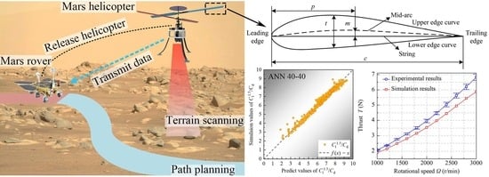
1. Introduction
2. Simulation and Machine Learning Methods
2.1. Two-Dimensional CFD Simulation Methods
2.2. Three-Dimension CFD Simulation Methods
2.3. Machine Learning Models
3. Results and Discussion
3.1. FEM Simulations
3.2. Regression Results of Different Algorithms
3.3. Evaluation of Different Algorithms
3.4. NACA Airfoil Optimization and ML Prediction
4. Mars Atmospheric Environment Simulation and Experiment
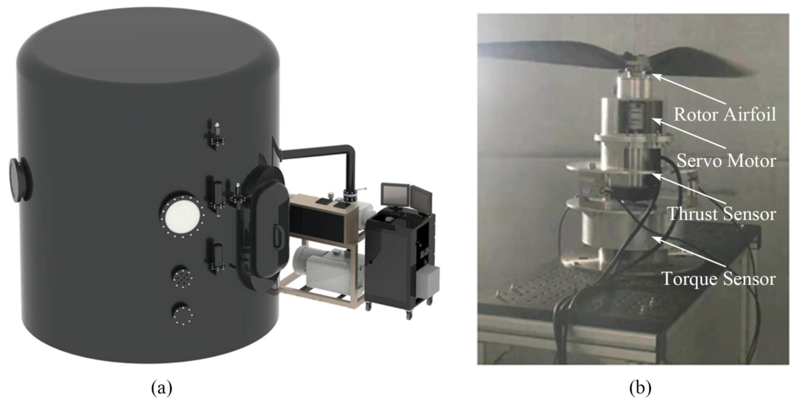
4.1. Experimental Device
4.2. Experiment Results
5. Conclusions
Author Contributions
Funding
Institutional Review Board Statement
Informed Consent Statement
Acknowledgments
Conflicts of Interest
References
- Crisp, J.A.; Adler, M.; Matijevic, J.R.; Squyres, S.W.; Arvidson, R.E.; Kass, D.M. Mars exploration rover mission. J. Geophys. Res. Planets 2003, 108. [Google Scholar] [CrossRef]
- Lindemann, R.A.; Voorhees, C.J. Mars Exploration Rover mobility assembly design, test and performance. In Proceedings of the 2005 IEEE International Conference on Systems, Man and Cybernetics, Waikoloa, HI, USA, 12 October 2005; Volume 1, pp. 450–455. [Google Scholar]
- Zhu, K.; Tang, D.; Quan, Q.; Lv, Y.; Shen, W.; Deng, Z. Modeling and experimental study on orientation dynamics of a Mars rotorcraft with swashplate mechanism. Aerosp. Sci. Technol. 2023, 138, 108311. [Google Scholar] [CrossRef]
- Zhu, K.; Quan, Q.; Wang, K.; Tang, D.; Tang, B.; Dong, Y.; Wu, Q.; Deng, Z. Conceptual design and aerodynamic analysis of a Mars octocopter for sample collection. Acta Astronaut. 2023, 207, 10–23. [Google Scholar] [CrossRef]
- Takaki, R. Aerodynamic characteristics of naca4402 in low reynolds number flows. Jpn. Soc. Aeronaut. Space Sci. 2006, 54, 367–373. [Google Scholar]
- Sunada, S.; Sakaguchi, A.; Kawachi, K. Airfoil section characteristics at a low Reynolds number. J. Fluids Eng. 1997, 119, 129–135. [Google Scholar] [CrossRef]
- Srinath, D.; Mittal, S. Optimal airfoil shapes for low Reynolds number flows. Int. J. Numer. Methods Fluids 2009, 61, 355–381. [Google Scholar] [CrossRef]
- Selig, M.S.; McGranahan, B.D. Wind tunnel aerodynamic tests of six airfoils for use on small wind turbines. J. Sol. Energy Eng. 2004, 126, 986–1001. [Google Scholar] [CrossRef]
- Lin, J.M.; Pauley, L.L. Low-Reynolds-number separation on an airfoil. AIAA J. 1996, 34, 1570–1577. [Google Scholar] [CrossRef]
- Spedding, G.; McArthur, J. Span efficiencies of wings at low Reynolds numbers. J. Aircr. 2010, 47, 120–128. [Google Scholar] [CrossRef]
- Okamoto, M.; Azuma, A. Aerodynamic characteristics at low Reynolds number for wings of various planforms. AIAA J. 2011, 49, 1135–1150. [Google Scholar] [CrossRef]
- Schafroth, D.; Bermes, C.; Bouabdallah, S.; Siegwart, R. Modeling and system identification of the mufly micro helicopter. In Proceedings of the Selected Papers from the 2nd International Symposium on UAVs, Reno, NV, USA, 8–10 June 2009; Springer: Berlin/Heidelberg, Germany, 2010; pp. 27–47. [Google Scholar]
- Chen, C.; Chen, B.M.; Lee, T. Special issue on development of autonomous unmanned aerial vehicles. Mechatronics 2011, 21, 763–764. [Google Scholar] [CrossRef]
- Bleischwitz, R.; de Kat, R.; Ganapathisubramani, B. Aspect-ratio effects on aeromechanics of membrane wings at moderate Reynolds numbers. AIAA J. 2015, 53, 780–788. [Google Scholar] [CrossRef]
- Mizoguchi, M.; Itoh, H. Effect of aspect ratio on aerodynamic characteristics at low Reynolds numbers. AIAA J. 2013, 51, 1631–1639. [Google Scholar] [CrossRef]
- Kruyt, J.W.; Van Heijst, G.F.; Altshuler, D.L.; Lentink, D. Power reduction and the radial limit of stall delay in revolving wings of different aspect ratio. J. R. Soc. Interface 2015, 12, 20150051. [Google Scholar] [CrossRef] [PubMed] [Green Version]
- Hassanalian, M.; Throneberry, G.; Abdelkefi, A. Wing shape and dynamic twist design of bio-inspired nano air vehicles for forward flight purposes. Aerosp. Sci. Technol. 2017, 68, 518–529. [Google Scholar] [CrossRef]
- Leishman, J.G. Aerodynamic optimization of a coaxial proprotor. In Proceedings of the The American Helicopter Society 62nd Annual Forum, Phoenix, AZ, USA, 9–11 May 2006. [Google Scholar]
- Bohorquez, F.; Pines, D.; Samuel, P.D. Small rotor design optimization using blade element momentum theory and hover tests. J. Aircr. 2010, 47, 268–283. [Google Scholar] [CrossRef]
- Benedict, M.; Winslow, J.; Hasnain, Z.; Chopra, I. Experimental investigation of micro air vehicle scale helicopter rotor in hover. Int. J. Micro Air Veh. 2015, 7, 231–255. [Google Scholar] [CrossRef] [Green Version]
- Shrestha, R.; Benedict, M.; Hrishikeshavan, V.; Chopra, I. Hover performance of a small-scale helicopter rotor for flying on mars. J. Aircr. 2016, 53, 1160–1167. [Google Scholar] [CrossRef]
- Song, X.; Wang, L.; Luo, X. Airfoil optimization using a machine learning-based optimization algorithm. J. Phys. Conf. Ser. 2022, 2217, 012009. [Google Scholar] [CrossRef]
- Du, Q.; Liu, T.; Yang, L.; Li, L.; Zhang, D.; Xie, Y. Airfoil design and surrogate modeling for performance prediction based on deep learning method. Phys. Fluids 2022, 34, 015111. [Google Scholar] [CrossRef]
- Li, K.; Kou, J.; Zhang, W. Unsteady aerodynamic reduced-order modeling based on machine learning across multiple airfoils. Aerosp. Sci. Technol. 2021, 119, 107173. [Google Scholar] [CrossRef]
- Zhang, Y.; Sung, W.J.; Mavris, D.N. Application of convolutional neural network to predict airfoil lift coefficient. In Proceedings of the 2018 AIAA/ASCE/AHS/ASC Structures, Structural Dynamics, and Materials Conference, Kissimmee, FL, USA, 8–12 January 2018; p. 1903. [Google Scholar]
- Zhu, L.; Zhang, W.; Kou, J.; Liu, Y. Machine learning methods for turbulence modeling in subsonic flows around airfoils. Phys. Fluids 2019, 31, 015105. [Google Scholar] [CrossRef]
- Wang, X.; Dong, Z.; Tang, L.; Zhang, Q. Multiobjective multitask optimization-neighborhood as a bridge for knowledge transfer. IEEE Trans. Evol. Comput. 2022, 27, 155–169. [Google Scholar] [CrossRef]
- Wang, X.; Hu, T.; Tang, L. A multiobjective evolutionary nonlinear ensemble learning with evolutionary feature selection for silicon prediction in blast furnace. IEEE Trans. Neural Netw. Learn. Syst. 2021, 33, 2080–2093. [Google Scholar] [CrossRef] [PubMed]
- Koning, W.J.; Johnson, W.; Grip, H.F. Improved Mars helicopter aerodynamic rotor model for comprehensive analyses. AIAA J. 2019, 57, 3969–3979. [Google Scholar] [CrossRef] [Green Version]
- Bensignor, I.; Seth, D.; McCrink, M. Rotor Propulsion Modeling for Low Reynolds Number Flow (Re < 105) for Martian Rotorcraft Flight. In Proceedings of the AIAA AVIATION 2022 Forum, Chicago, IL, USA, 27 June–1 July 2022; p. 3958. [Google Scholar]
- Rajarajan, S.; Surya, P.; Karthikeyan, M.; Manikandan, P.; Lokeshkumar, K. Numerical Study of Unconventional Airfoils at Low Reynolds Number for the Application of Mars Flight. Int. J. Appl. Eng. Res. 2021, 16, 362–371. [Google Scholar]
- Moghadam, P.Z.; Rogge, S.M.; Li, A.; Chow, C.M.; Wieme, J.; Moharrami, N.; Aragones-Anglada, M.; Conduit, G.; Gomez-Gualdron, D.A.; Van Speybroeck, V.; et al. Structure-mechanical stability relations of metal-organic frameworks via machine learning. Matter 2019, 1, 219–234. [Google Scholar] [CrossRef] [Green Version]
- Rojas, R. Neural Networks: A Systematic Introduction; Springer Science & Business Media: Berlin/Heidelberg, Germany, 2013. [Google Scholar]
- Cortes, C.; Vapnik, V. Support-vector networks. Mach. Learn. 1995, 20, 273–297. [Google Scholar] [CrossRef]
- Otchere, D.A.; Ganat, T.O.A.; Gholami, R.; Ridha, S. Application of supervised machine learning paradigms in the prediction of petroleum reservoir properties: Comparative analysis of ANN and SVM models. J. Pet. Sci. Eng. 2021, 200, 108182. [Google Scholar] [CrossRef]
- Sobhani, J.; Khanzadi, M.; Movahedian, A. Support vector machine for prediction of the compressive strength of no-slump concrete. Comput. Concr. 2013, 11, 337–350. [Google Scholar] [CrossRef]
- Friedman, J.H. Greedy function approximation: A gradient boosting machine. Ann. Stat. 2001, 29, 1189–1232. [Google Scholar] [CrossRef]
- Drucker, H. Improving regressors using boosting techniques. Icml 1997, 97, 107–115. [Google Scholar]
- Schapire, R.E. The boosting approach to machine learning: An overview. In Nonlinear Estimation and Classification; Springer: Berlin/Heidelberg, Germany, 2003; pp. 149–171. [Google Scholar]
- Allen, D.M. Mean square error of prediction as a criterion for selecting variables. Technometrics 1971, 13, 469–475. [Google Scholar] [CrossRef]
- Quinino, R.C.; Reis, E.A.; Bessegato, L.F. Using the coefficient of determination R2 to test the significance of multiple linear regression. Teach. Stat. 2013, 35, 84–88. [Google Scholar] [CrossRef]


| Parameters | Values |
|---|---|
| Gas density () | 0.0167 |
| Constant pressure specific heat capacity (J/kg·K) | 831.2 |
| Thermal conductivity (W/m·K) | 0.0132 |
| Gas viscosity (kg/m·s) | |
| Reference viscosity (kg/m·s) | |
| Reference temperature (K) | 210 |
| Effective temperature (K) | 260 |
| Molar mass (g/mol) | 44 |
| Reference area () | 0.04 |
| Reference length (m) | 0.04 |
| Reference depth (m) | 1 |
| m | p | t | Relative Error (%) | ||||
|---|---|---|---|---|---|---|---|
| 0 | 5.41 | 6.28 | 4.00 | 8.028 | 8.065 | 8.035 | 0.37 |
| 1 | 5.33 | 6.29 | 4.00 | 9.056 | 9.089 | 9.083 | 0.06 |
| 2 | 4.54 | 7.81 | 4.00 | 9.816 | 9.835 | 9.829 | 0.06 |
| 3 | 4.31 | 7.85 | 4.00 | 10.263 | 10.312 | 10.304 | 0.08 |
| 4 | 4.25 | 7.85 | 4.00 | 10.363 | 10.454 | 10.423 | 0.30 |
| 5 | 4.21 | 7.85 | 4.00 | 10.285 | 10.391 | 10.352 | 0.38 |
| 6 | 4.19 | 7.85 | 4.00 | 10.060 | 10.184 | 10.103 | 0.80 |
| 7 | 4.16 | 7.86 | 4.00 | 9.796 | 9.974 | 9.809 | 1.69 |
| 8 | 4.20 | 7.76 | 4.00 | 9.653 | 9.732 | 9.655 | 0.80 |
| 9 | 4.50 | 7.55 | 4.36 | 8.915 | 8.931 | 8.935 | −0.05 |
| 10 | 5.40 | 6.28 | 4.27 | 8.249 | 8.250 | 8.255 | −0.07 |
| m | p | t | Relative Error (%) | ||||
|---|---|---|---|---|---|---|---|
| 0 | 6.48 | 7.65 | 4.00 | 4.644 | 4.650 | 4.652 | −0.05 |
| 1 | 6.51 | 7.61 | 4.00 | 5.822 | 5.829 | 5.836 | −0.12 |
| 2 | 6.29 | 7.76 | 4.00 | 6.773 | 6.816 | 6.777 | 0.57 |
| 3 | 5.98 | 7.84 | 4.00 | 7.465 | 7.525 | 7.481 | 0.58 |
| 4 | 5.34 | 7.89 | 4.00 | 7.934 | 7.988 | 7.961 | 0.33 |
| 5 | 4.64 | 7.93 | 4.00 | 8.311 | 8.361 | 8.316 | 0.54 |
| 6 | 4.39 | 7.95 | 4.00 | 8.576 | 8.617 | 8.612 | 0.06 |
| 7 | 4.32 | 7.94 | 4.00 | 8.797 | 9.000 | 8.813 | 2.12 |
| 8 | 4.31 | 7.87 | 4.00 | 9.315 | 9.396 | 9.338 | 0.63 |
| 9 | 5.25 | 7.89 | 4.00 | 9.160 | 9.161 | 9.189 | −0.31 |
| 10 | 6.22 | 7.91 | 4.00 | 8.881 | 8.886 | 8.904 | −0.20 |
| m | p | t | Relative Error (%) | |||
|---|---|---|---|---|---|---|
| 0.5 | 5.39 | 6.17 | 4.00 | 8.559 | 8.654 | −1.11 |
| 1.5 | 4.77 | 7.74 | 4.04 | 9.481 | 9.422 | 0.63 |
| 2.5 | 4.40 | 7.80 | 4.11 | 10.186 | 10.010 | 1.75 |
| 3.5 | 4.31 | 7.80 | 4.15 | 10.538 | 10.278 | 2.54 |
| 4.5 | 4.28 | 7.80 | 4.17 | 10.536 | 10.257 | 2.71 |
| 5.5 | 4.25 | 7.81 | 4.18 | 10.373 | 10.075 | 2.96 |
| 6.5 | 4.17 | 7.85 | 4.16 | 10.065 | 9.815 | 2.54 |
| 7.5 | 4.16 | 7.83 | 4.17 | 9.870 | 9.703 | 1.72 |
| 8.5 | 4.28 | 7.63 | 4.26 | 9.359 | 9.315 | 0.46 |
| 9.5 | 5.44 | 7.91 | 4.25 | 8.504 | 8.558 | −0.64 |
| m | p | t | Relative Error (%) | |||
|---|---|---|---|---|---|---|
| 0.5 | 5.71 | 6.98 | 4.00 | 5.188 | 5.216 | −0.54 |
| 1.5 | 5.96 | 8.00 | 4.00 | 6.341 | 6.343 | −0.03 |
| 2.5 | 5.94 | 7.86 | 4.00 | 7.047 | 7.168 | −1.68 |
| 3.5 | 5.96 | 7.85 | 4.09 | 7.683 | 7.722 | −0.50 |
| 4.5 | 4.62 | 7.87 | 4.12 | 8.126 | 8.063 | 0.79 |
| 5.5 | 4.47 | 7.86 | 4.15 | 8.557 | 8.327 | 2.77 |
| 6.5 | 4.31 | 7.88 | 4.15 | 8.828 | 8.517 | 3.65 |
| 7.5 | 4.29 | 7.85 | 4.17 | 9.347 | 8.933 | 4.63 |
| 8.5 | 4.44 | 7.77 | 4.25 | 9.473 | 9.201 | 2.96 |
| 9.5 | 5.74 | 7.81 | 4.25 | 9.232 | 8.995 | 2.63 |
Disclaimer/Publisher’s Note: The statements, opinions and data contained in all publications are solely those of the individual author(s) and contributor(s) and not of MDPI and/or the editor(s). MDPI and/or the editor(s) disclaim responsibility for any injury to people or property resulting from any ideas, methods, instructions or products referred to in the content. |
© 2023 by the authors. Licensee MDPI, Basel, Switzerland. This article is an open access article distributed under the terms and conditions of the Creative Commons Attribution (CC BY) license (https://creativecommons.org/licenses/by/4.0/).
Share and Cite
Zhao, P.; Gao, X.; Zhao, B.; Liu, H.; Wu, J.; Deng, Z. Machine Learning Assisted Prediction of Airfoil Lift-to-Drag Characteristics for Mars Helicopter. Aerospace 2023, 10, 614. https://doi.org/10.3390/aerospace10070614
Zhao P, Gao X, Zhao B, Liu H, Wu J, Deng Z. Machine Learning Assisted Prediction of Airfoil Lift-to-Drag Characteristics for Mars Helicopter. Aerospace. 2023; 10(7):614. https://doi.org/10.3390/aerospace10070614
Chicago/Turabian StyleZhao, Pengyue, Xifeng Gao, Bo Zhao, Huan Liu, Jianwei Wu, and Zongquan Deng. 2023. "Machine Learning Assisted Prediction of Airfoil Lift-to-Drag Characteristics for Mars Helicopter" Aerospace 10, no. 7: 614. https://doi.org/10.3390/aerospace10070614