Article

On the Self-Similarity in an Annular Isolator under Rotating Feedback Pressure Perturbations

1
Jiangsu Province Key Laboratory of Aerospace Power System, College of Energy and Power Engineering, Nanjing University of Aeronautics and Astronautics, Nanjing 210016, China
2
National Key Laboratory of Transient Physics, Nanjing University of Science and Technology, Nanjing 210094, China
3
Science and Technology on Space Physics Laboratory, Beijing 100076, China
*
Authors to whom correspondence should be addressed.
Aerospace 2023, 10(2), 188; https://doi.org/10.3390/aerospace10020188
Submission received: 31 December 2022 / Revised: 12 February 2023 / Accepted: 14 February 2023 / Published: 16 February 2023
(This article belongs to the Special Issue Thermal Fluid Dynamics and Control in Aerospace)

Abstract

:
In this paper, the transient flow simulation in an annular isolator under rotating feedback pressure perturbations simplified from the rotating denotation wave (RDW) is performed. The instantaneous flow characteristics and the self-similarity of the isolator flow-field are investigated in detail. It is found that a helical moving shock wave (MSW) and a quasi-toroidal terminal shock wave (TSW) are induced in the isolator. Hence, the flow-fields on the meridian planes could be classified into three zones, i.e., the undisturbed zone, the terminal shock wave/moving shock wave/boundary layer interaction (TSW/MSW/BLI) zone and the moving shock wave/boundary layer interaction (MSW/BLI) zone. The TSW/MSW/BLI zone is characterized by the coupling of the TSW/BLI and the MSW/BLI due to their small axial distance, which intensifies the adverse pressure gradient on the meridian planes, thus rolling up large separation bubbles developing along the MSW driven by the circular pressure gradient. In the MSW/BLI zone, the shock induces the boundary layer to separate, forming a helical vortex located at the foot of the MSW. During the upstream propagation process, the pattern of the MSWs transforms from a moving normal shock wave to a moving oblique shock wave with decreased strength. Moreover, after the collision with the MSWs, P, Temp and S of the flow elevate with the prompt decrease of va, while vθ increases to a higher level. Despite the deflection effect of the MSWs on the streamlines, the flow direction of the air still maintains an almost axial position at the exit, except in the adjacent region of the MSW. Likewise, three types of zones can be determined in the flow pattern at the exit: the rotating detonation wave/boundary layer interaction (RDW/BLI) zone, the expansion zone, and the vortices discharge zone. Comparing the transient flow patterns at different moments in one cycle and between adjacent cycles, an interesting discovery is that the self-similarity property is observed in the flow-field of the annular isolator under rotating feedback pressure perturbations. The global flow structure of the isolator at different moments shows good agreement despite its rotation with the RDW, and the surface pressure profiles of the corresponding meridian planes all match perfectly. Such a characteristic indicates that the rotation angular velocity of the TSW and the MSW are equal and hold invariant, and the isolator flow could be regarded as a quasi-steady flow. On this basis, the theoretical model of the inclination angles of the MSW by the coordinate transformation and velocity decomposition is developed and validated. The relative errors of the inclination angles between the predicted and measured results are below 3%, which offers a rapid method to predict the shape of the MSW, along with a perspective to better understand the physical meaning of the shape of the MSW.

1. Introduction

Due to the potential benefits of high thermal efficiency, rapid heat release and compact combustor, the rotating detonation engine (RDE) has attracted growing attention in recent years [1,2,3]. In a typical air-breathing rotating detonation combustor (RDC), a detonation wave propagates circumferentially along the annular combustor, ensuring the stability and continuity of detonative combustion [4]. As a critical component of the rotating detonation ramjet/scramjet engine (RDRE/RDSE), the isolator plays a key role in isolating the aerodynamic and thermal perturbations propagating upstream from the RDC and preventing the inlet from unstart [5,6]. Unlike the conventional deflagration combustion, the feedback pressure perturbations induced by the rotating detonation wave (RDW) propagates upstream in the axial and circumferential directions periodically, with a frequency of 1–10 kHz and an ultra-high amplitude [7]. These feedback pressure perturbations induce a helical moving shock wave (MSW) in the isolator, which interacts with the boundary layer and the terminal shock wave (TSW), thus directly affecting the aerodynamic performance of the inlet/isolator and the operating characteristics of the RDE, bringing great challenges to the design of the isolator. Hence, it is of great importance to investigate in depth the flow characteristics in the isolator under rotating feedback pressure perturbations with high frequency and amplitude.
Since the concept of rotating detonation proposed by Voitsekhovskii in the 1960s, [8] a series of studies have been carried out on flow characteristics in air-breathing RDCs. Zhdan [9] and Zhu [10] numerically studied the two-dimensional flow structure of hydrogen-oxygen RDC and carbon-air RDC, respectively. Two-dimensional and three-dimensional simulations on the RDC of H2/O2 and H2/air were conducted by Uemura, and the detonation mechanism and related dynamics of the RDC were analyzed in a subtle way [11]. Rui tracked the paths of flow particles in a two-dimensional RDC, and evaluated the effect of the wave system of the detonation on the paths [12]. Smirnov [13,14] reconstructed the flow-field of the RDC, and the effect of the different equivalence ratios of the mixture on the modes of the RDW was analyzed. A common finding in experimental studies is that the variation of the operating conditions seems to result in the transition of propagation modes of the RDW, which could be mainly classified as the single wave mode, the multiple waves mode, the contrarotating waves mode, and the colliding waves mode, etc. [15,16,17,18,19]. Moreover, the RDW instability is another critical issue in the RDC flow-field investigations, a various types of which have been confirmed and analyzed in both experiments and simulations [20,21,22,23,24].
As a matter of common knowledge, the rotating feedback pressure perturbations propagating upstream from the RDC is one of the key factors affecting the flow structure and performance of the isolator, which have been observed by both simulations and experiments [16,25,26,27]. For the rotating detonation based aero-turbine engine, the isolator [28,29,30] is utilized and studied to dampen the effect of the feedback pressure on the compressor, the inflow of which is determined both by the inlet and compressor. In the isolator of a ramjet/scramjet-type RDE, where no compressor or turbine exists, the feedback pressure propagation from the RDC induces the upstream oblique shock wave (OSW), i.e., the helical MSW in the isolator, fairly affecting the characteristics of the isolator flow-field. The three-dimensional simulations conducted by Liu showed that the location of the upstream OSW would be affected by the total temperature and velocity of the inflow [31]. Furthermore, they validated the existence of the pressure feedback of the upstream OSW in the experiments [32]. In the numerical study by Dubrovskii, [33] due to the supersonic condition of the inflow, the pressure feedback could not propagate upstream to the isolator, two OSWs cycled along with the RDW in the combustor instead. Zhao [34] numerically explored the upstream influence of the RDW on the supersonic inlet, proposing that the TSW appears to adjust its location and strength with time in the diffuser. Wu performed the simulations of the RDE with a direct-connect Laval nozzle [35]. Their study indicated that the unsteady upstream OSW may destroy the internal flow of the RDE, ultimately affecting the fuel intake. On this basis, they further applied the particle trajectory method to investigate the influence of the OSWs on particle behavior and evaluated the pressure gain performance in detail [36].
From the literature, it is understood that the previous studies on feedback pressure and the upstream OSW are mainly focused on their impacts on the flow-field and operation of the RDC. The flow-field structure in the isolator under rotating feedback pressure perturbations and the mechanism of the interaction between the helical MSW and the boundary layer have not been thoroughly understood. Nevertheless, the propagation of the rotating feedback pressure perturbations and the moving shock wave/boundary layer interaction (MSW/BLI) would break the original axial symmetry of the isolator flow, enhancing the three-dimensionality and unsteadiness of the flow-field, making it extremely complex. This undoubtedly could have great influence on the thermal and aerodynamic performance of the RDE, thus requiring further studies. In addition, the issue on the self-similarity property of the isolator flow-field under such conditions has not been addressed and discussed. Furthermore, The theoretical model of the inclination angles of the MSW has never been developed. Therefore, in this paper, the above undisclosed flow characteristics in an annular isolator under rotating feedback pressure perturbations are investigated in depth, aiming to fill such a gap in the existing knowledge, and provide a theoretical basis for the isolator design of the RDE.
This paper is built on previous studies and is hereby, organized as follows. First, Section 2 and Section 3 introduce the physical model of the isolator studied and the relevant details of the numerical setup in sequence. On this basis, the transient isolator flow characteristics under simplified rotating feedback pressure perturbations is discussed in detail in Section 4, which also details the terminal shock wave/helical moving shock wave/boundary layer interaction (TSW/MSW/BLI), along with the impacts of the terminal shock wave and the moving shock wave on the main flow and the flow patterns at the exit. Then, the spatial-temporal self-similarity property in the isolator flow-field at such a condition is discovered and discussed in Section 5. Then, in Section 6, a theoretical prediction method of the inclination angle of the helical MSW is put forward, based on the velocity decomposition method, and compared with the numerical result. Ultimately, the important results and findings obtained from the current study are discussed in Section 7.

2. Physical Model of the Isolator

The curved meridian plane of the co-axial annular isolator model studied in this paper is schematically presented in Figure 1, of which the length Liso is 228.43 mm, the height of the entrance Hent and the exit Hexi is 12 mm and 14 mm, respectively. In addition, the inner radius of the entrance Rent-in and the exit Rexi-in of the isolator is 152.28 mm and 143 mm in sequence. Table 1 summarizes the specific geometric parameters of the isolator.
The isolator comprises two sections, that is, the S-shaped section and the straight terminal section with constant cross-section. The quadruplicate polynomial is utilized as the centerline function of the S-shaped section shown in Equation (1), where x varies from 0 to LS-shaped (the length of the S-shaped section, which is 208.43 mm) and Roff,iso refers to the radial offset of the isolator equivalent to that of the S-shaped section:
r ( R ent - in + 0.5 H ent ) R off , iso = 4 ( x L S - shaped ) 3 + 3 ( x L S - shaped ) 4
In addition, the duct height H (which is defined as the radial difference between the outer and inner wall) distribution function of the S-shaped section along the axis are a cubic polynomial, as shown in Equation (2):
H = [ 3 ( x L S - shaped ) 2 2 ( x L S - shaped ) 3 ] ( H e x i H ent ) + H ent ,

3. Methodology

3.1. Numerical Methods

Since the unsteady shock wave system/boundary layer interaction plays a vital role in the isolator study, a reliable numerical method that can capture the unsteady motion of the shock waves accurately is quite essential. In this paper, the three-dimensional unsteady compressible RANS equations are solved via the computational fluid dynamic software ANSYS FLUENT, which is based on the finite volume method. The turbulence is modeled by the κω SST model, [37] while the piecewise polynomial method and the Sutherland model are selected to compute the specific heat and the viscosity coefficient, separately. All of the flow equations are discretized both spatially and temporally with second-order accuracy and the Green–Gauss cell based gradient approximation is adopted. In addition, unsteady flow solutions are sought at a fine time step of Δt = 2 × 10⁻⁷ s with 45 iterations per time step, which is 1 × 10⁻³ times of the cycle T (equaling to 2 × 10⁻⁴ s) of rotating feedback pressure perturbations. During calculation, the mass flow, the Mach number and the total pressure at the exit are monitored, along with the residuals. An absolute convergence criterion of 10−5 is satisfied at every time step in the continuity equation’s scaled-residuals.
The computational domain shown in Figure 2a is all filled with hexahedral cells, and the near-wall grids are all encrypted with the spacing of 0.01 mm, ensuring the most of the y+ and z+ values are kept below 1. The details in the mesh sensitivity study are presented in Section 3.3. In addition, three primary metrics to evaluate the quality of the grids generated are paid special attention here, which are aspect ratio, equiangle skewness, and orthogonal quality. The aspect ratio is a measure of the stretching of the elements, which is referred to as the ratio of the lengths of the largest and the smallest edge, for the three-dimensional cell utilized here. The minimum value of the aspect ratio is 1.64 while the maximum is 179.18. The average value is 27.77, which is quite below the threshold of 100. The equiangle skewness is one of the primary measures determining how close a face or a cell is to the equilateral, affecting the accuracy and stability of the calculation. The maximum value of the grid is 0.049, the minimum is 0.003, and the average is 0.024, which is quite close to 0. The orthogonal quality ranges from 0 to1. When the orthogonal quality is closer to 1, the best quality of the grid is defined. The minimum orthogonal quality for all cells is 0.988, which is extremely close to 1. Hence, the quality of the grid used in this paper is rather good.
As shown is Figure 2b, there are three types of boundary conditions utilized in this paper. The computational entrance is set as the pressure far field, and the exit of the isolator is set as the pressure outlet. Moreover, the inner and outer walls are set as an adiabatic non-slip wall. In this study, the incoming flow conditions are listed in Table 2, and the distribution of which is given by a profile calculated from an axisymmetric inlet with the design Mach number of 5 at the flight height of 24 km. Accordingly, the freestream pressure P0 of the inlet/isolator is 2971.75 Pa. The inflow static pressure Pent in Table 2 is normalized against P0.

3.2. Implementation of Rotating Feedback Pressure Perturbations

As mentioned in Section 1, the RDW alters the flow-field in the isolator essentially via the upstream propagation of its rotating feedback pressure perturbations. Hereby, imposing the unsteady pressure with the key properties of the RDW on the exit of the isolator would be a reasonable simplified simulation method, [38,39] instead of a real RDW, as the emphasis of this paper is placed on the effects of the rotating feedback pressure propagation on the isolator flow-field. Primarily, the radial discrepancy of the feedback pressure is ignored as Hexi << Rexi-in and Hent << Rent-in. Moreover, the instabilities of the RDW are neglected [40], which renders the simplified RDW periodical.
As the RDW sweeps over the pressure transducer at the exit, the measured value increases steeply to a peak value and then falls back to the valley value at a relatively gentle rate [41]. In addition, since only the single RDW mode is considered here, the spatial distribution of the static pressure around the exit is essentially the same as the temporal distribution of the static pressure in a certain radial column of cell faces at the exit, despite the difference on the independent variable and the corresponding phase difference. Thus, a simplified model of the RDW is developed [38,39,42].
The column of cell faces with the azimuthal angle θ equaling 180° and named as the 1st column is chosen as an example to introduce the temporal function of the simplified model. The rotating frequency of the RDW is set to 5 kHz, a linear function is selected to model the ascent stage of the feedback pressure in one cycle given by Equation (3):
P b , 1 p 0 = 45.92 ( 100 t T ) + 104.6
where Pb,1 denotes the feedback pressure for the 1st column of cell faces at the exit, and t/T ranges from 0 to 0.0382. The subsequent steep drop of Pb,1 is also given by a linear function, as follows:
P b , 1 p 0 = 13.09 × ( 100 t T ) + 330
where t/T is from 0.0382 to 0.1146. Then, the final slight descending of Pb,1 is given by a trigonometric function with an exponential function as its independent variable listed in Equation (5), where the corresponding t/T is from 0.1146 to 1:
P b , 1 p 0 = 156.64 sin ( π e 0.02 k ) + 104.6
where
k = m t T
In Equation (6), m is defined as the magnification factor, equivalent to 800 in this study.
Figure 3 presents the spatial distribution and the time-varying curve of the feedback pressure computed by Equations (3)–(5). The main parameters of the feedback pressure perturbations at the exit Pb are presented in Table 3, among which the pressure parameters are all non-dimensionalized by P0.

3.3. Validation of the Numerical Method and Grid Sensitivity Verification

The capability of describing the unsteady shock wave propagation of the numerical approach adopted hereinafter is inspected with the experimental results in [43], where a planar shock wave is transmitted in a 90° branched duct with a rectangular cross section (20 mm in height, and 40 mm in width). The propagation Mach number of the original shock wave Ms is 2.4 before its diffraction around the 90° sharp corner, when the pre-shock static pressure and temperature are 100 kPa and 288.15 K, respectively. Hence, the pressure ratio of the moving shock is about 6.55. The comparison of the shock wave structure between the experimental and numerical schlieren images are exhibited in Figure 4, the former of which was obtained with a 24 frame Cranz-Schardin spark camera, that clearly shows that there are no movable parts in the light ray’s path. The experimental shock tube possesses a test section equipped with plane, parallel windows of high optical quality glass. The optical field of view is 200 mm∙110 mm with the depth of 40mm [44]. As can be noted from the schlieren images, there is no significant disparity between the experiment and simulation from the perspectives of the shock wave structure. Consequently, the numerical method introduced above has a good accuracy in capturing the moving shock wave in a restricted duct.
For the purpose of verifying the grid convergence, three-dimensional structured grids in the isolator designed in Section 2 are generated with three different grid densities: the coarse grid (3 million cells), the fine grid (6 million cells), and the dense grid (9 million cells). Figure 5 compares the computed outer-wall pressure distribution of the isolator along the x-direction under an unthrottled state, the incoming flow condition of which is listed in Table 2. As it can be seen, the pressure curve of the fine grid is basically consistent with that of the dense grid, while the coarse case shows a tiny inequality in the region where the internal shock impinges on the walls. Hereby, the fine grid is utilized for the rest of the analysis in this paper.

4. Transient Flow Characteristics in the Isolator Affected by the Rotating Feedback Pressure

Since the isolator is an axisymmetric duct with steady and circumferentially uniform inflow conditions at the entrance and cyclical conditions of the rotating feedback pressure at the exit, it is rational to presume that the flow behaviors in the isolator during the stable operating stage would present a high periodicity as well, which will be discussed minutely in Section 5. Therefore, the instantaneous flow-field at the initial time of a certain cycle (i.e., t = nT, or floor (t, T) = 0) during the stable operating stage is firstly selected and analyzed in this section.

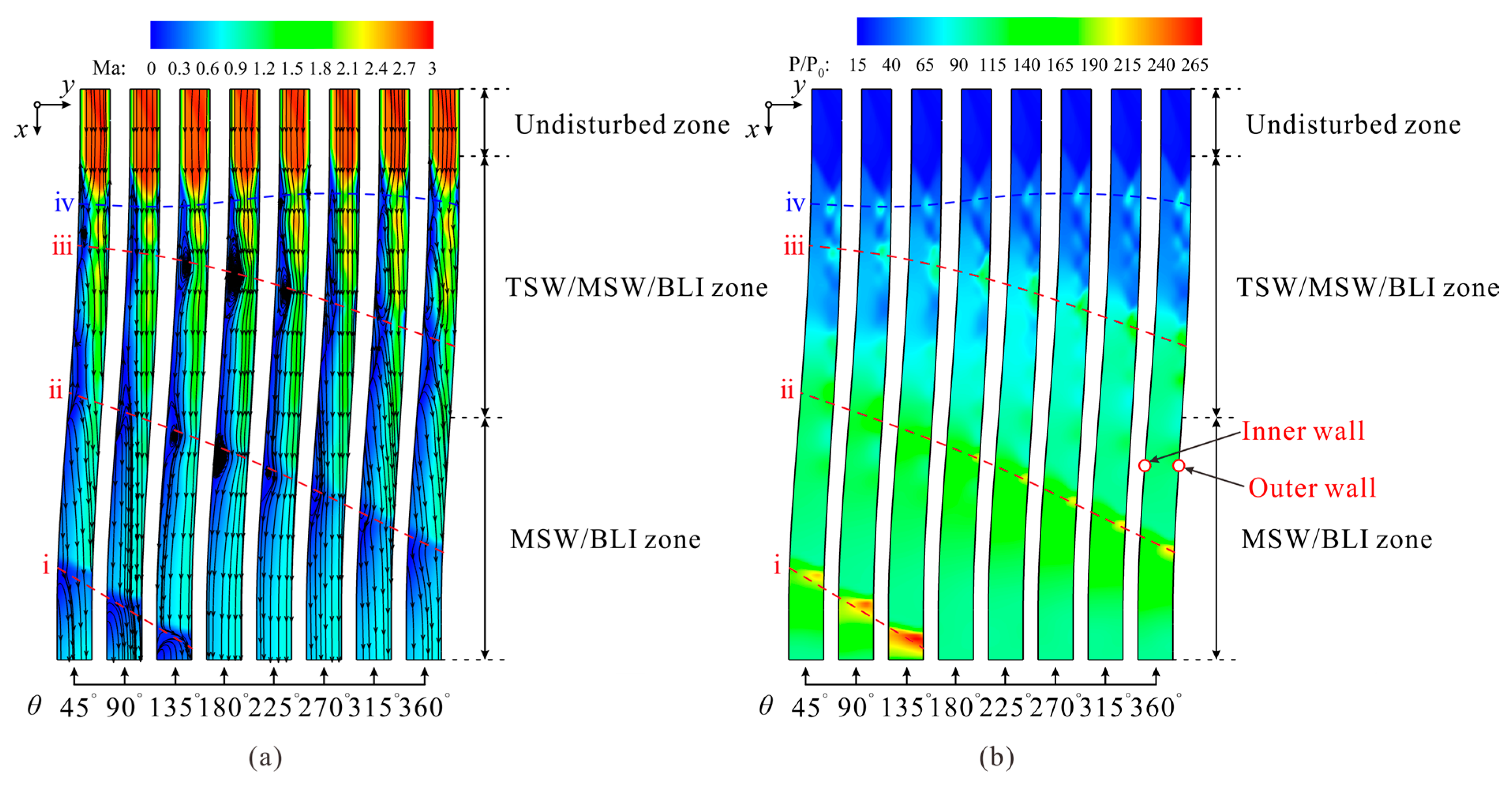
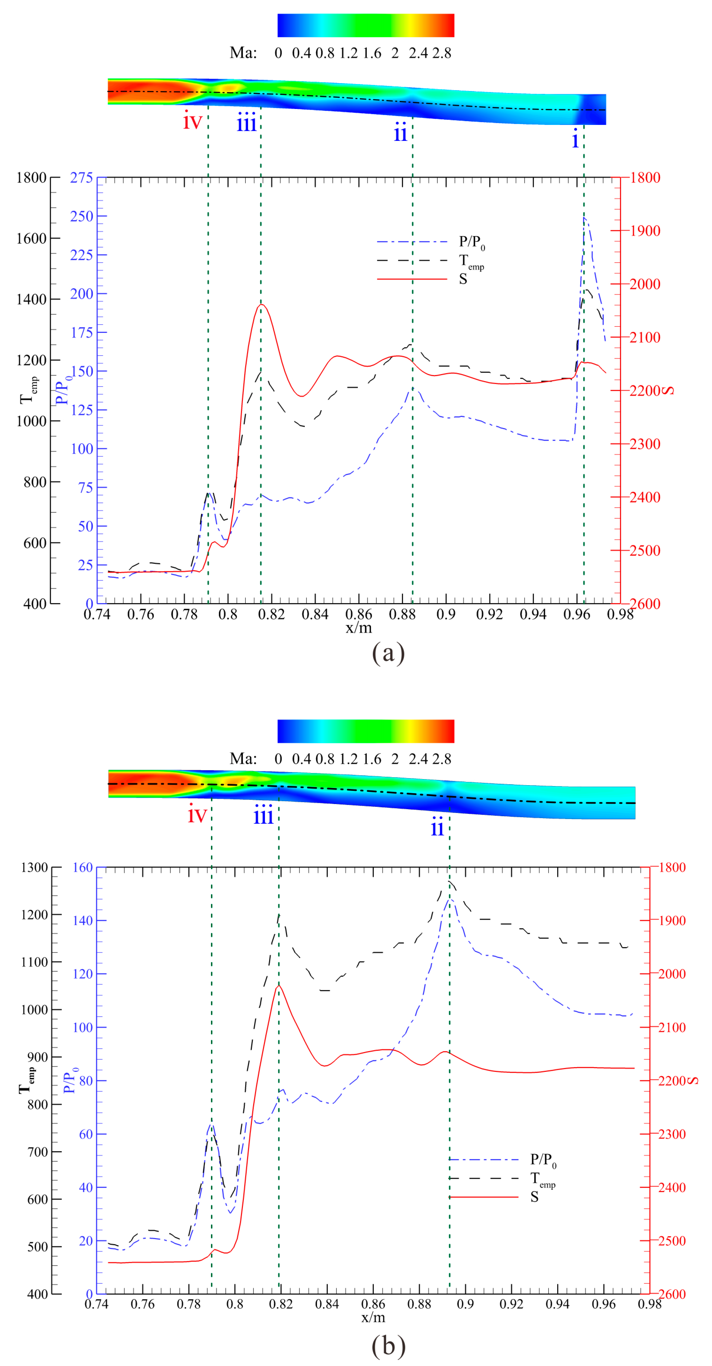
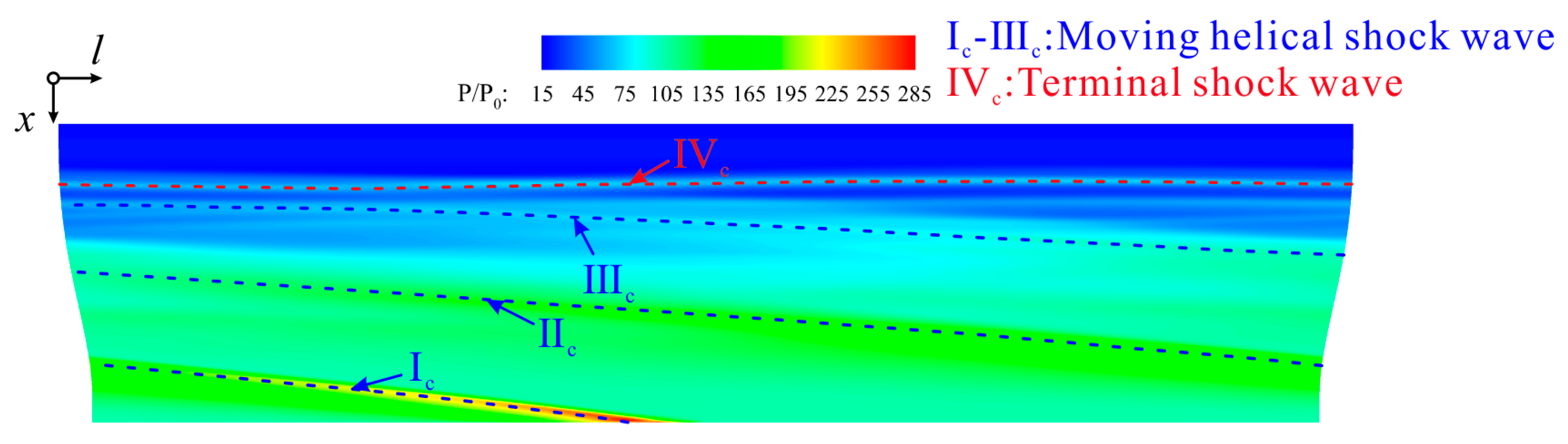
4.1. Terminal Shock Wave/Moving Shock Wave/Boundary Layer Interaction

Figure 6a,b present the pressure contours transformed into rectangular planes on the outer and inner wall of the isolator, respectively. The rotating feedback pressure perturbations induce a forward and circumferential motion of the helical moving shock wave (MSW) in the isolator, as indicated in Figure 6c. As the high-pressure perturbations propagate forward, the strength of the MSW attenuates gradually, the screw-pitch of the MSW reduces slightly, and the inclination angle between the MSW and the x-axis increases gently. In other words, the MSW shows more “flat” patterns along the negative direction of the x-axis. For facilitating the analysis, the helical MSWs on the walls are converted into multiple segments of curved MSWs on the x-θ plane, as indicated by blue arrows in Figure 6a,b. It can be observed that the MSWs on the outer wall appear stronger than those on the inner wall. This is mainly determined by the curvature effect of the walls [45], since the outer wall of the annular duct compresses the inflow and enhances the MSWs; while the flow near the inner wall tends to expand, thus weakening the MSWs. Moreover, the time-average feedback pressure equaling 114.95 P0 at the exit also induces a quasi-toroidal terminal shock wave (TSW) marked by red arrows in Figure 6a,b. Due to the rotation of the feedback pressure, the TSW oscillates in the x direction as the θ varies, which differs from that in the axisymmetric isolator under steady and uniform backpressure. [46] Though a series of expansion waves are generated downstream of the MSWs, the pressure along the axis-direction in the isolator still presents an overall ascending trend.
In an effort to visualize the terminal shock wave/moving shock wave/boundary layer interaction (TSW/MSW/BLI) intuitively, the flow-fields on eight meridian planes with equidifferent angles are rotated and shifted to the corresponding positions on the same x-y plane, as shown in Figure 7. It should be noted that the dashed lines in Figure 7 represents the curve of the shock waves with the angle, instead of the actual shock patterns in the meridian planes. Due to the circumstantial and axial curvature effects, the pressure on the outer wall is higher than that on the inner wall in Figure 7b, as observed in Figure 6a,b, and the low-momentum flow accumulates to the inner wall eventually after the first bend. As shown in Figure 7, the flow-fields could be classified into three zones, i.e., the undisturbed zone, the TSW/MSW/BLI zone dominated by the TSW indicated by blue dashed line iv, and the MSW indicated by the red dashed line iii, and the MSW/BLI zone, where only the MSWs indicated by red dashed lines i and ii exist. In the undisturbed zone, the streamlines are not affected by the TSW and the MSW downstream, and basically parallel to the x-axis. A coupling of the terminal shock wave/boundary layer interaction (TSW/BLI) and the moving shock wave/boundary layer interaction (MSW/BLI) takes place in the TSW/MSW/BLI zone. On the meridian planes with azimuthal angle θ ranging from 45° to 180°, the axial distance between the TSW and MSW iii is rather small, resulting in the enhanced coupling of the adverse pressure gradient generated from two shock waves, thus rolling up large separation bubbles developing along MSW iii driven by the circular pressure gradient. This migration of separation bubbles contributes to the maximum separation zone scale on the meridian plane at θ = 180°. While on the meridian planes with θ ranging from 225° to 360°, the axial distance between the two shock waves augments as the azimuthal angle increases, and the strength of the pressure gradient coupling drops, along with the shrinking of the separation bubbles. As for the MSW/BLI zone affected by MSW ii, with the counterflow in the vicinity of the inner wall, the separation bubbles and the streamline deflections occur successively in the region with θ ranging from 45° to 360°. Else, MSW i with the maximal strength turns the entire inflow in the reverse direction at θ = 135°, which is quite different from the steady shock/boundary layer interaction. An interesting discovery is that notwithstanding the deflecting effect the MSWs have on the flow, the flow direction of air still remains axial upstream of the exit, except in the adjacent region of MSW i. This undoubtedly will provide a favorable impact on the detonation combustion organization in the RDC.
The surface pressure distribution curves and the secondary flow patterns on the meridian plane at θ = 135° are extracted to obtain more details about the TSW/MSW/BLI, as depicted in Figure 8. During the process of propagation, the MSWs are weakened from the moving normal shock wave to the moving oblique shock wave, and eventually merge with the TSW. It can be seen that the pressure on the inner wall varies more smoothly than that on the outer wall, and a phase difference between the inner and outer surface pressure appears at the peak generated by MSW i. Whereas, no phase difference arising at the peak of MSW ii and iii can be noticed, which means that the velocity difference of the MSW’s upstream propagation and the flow on two sides of the walls counteract each other. Pressure oscillations on the outer wall can be found, which correspond to the collision between the airflow and the outer wall, as exhibited in Figure 8. This flow migration is caused by the vortices rolled up by the TSW/MSW/BLI and the MSW/BLI located around MSW ii, while the MSW/BLI caused by MSW i forms a separation line resembling a semi-circle and a reattachment line shaped as a straight line.
The spatial streamlines originated from the points at eight azimuthal angles (θ = 45°, 90°, 135°, 180°, 225°, 270°, 315°, and 360°) at the entrance are traced forward, the target of which is to portray and investigate the vortex structure induced by the TSW/MSW/BLI. The tracked streamlines can be divided into three types: the main flow streamlines emphasized by red lines in Figure 9a,b, the low-momentum flow streamlines near the outer wall emphasized by blue lines in Figure 9a, and the low-momentum flow streamlines near the inner wall emphasized by blue lines in Figure 9b. As shown in Figure 9, the streamlines of the main flow with a high momentum present a negligible lateral motion in the circumferential direction but slightly lifts and dives in the radial direction, due to the separation bubbles. It is interesting to note that the vortices generated from the boundary layer near both sides of walls all develop along the TSW and the MSWs, as shown in Figure 9 (the vortices shown in Figure 9c are identified by the Liutex-ΩR criterion proposed in [47,48] with the value of ΩR = 0.6 in yellow). The motivation of the circular motion of the vortices are the circular pressure gradient contributed by the inclination of the shock waves, which is a typical glancing shock wave/boundary layer interaction (GSW/BLI) [49,50]. In addition, the scales of the vortices show some disparity between the vicinity of the outer and inner walls, which corresponds to the flow-fields in Figure 7a. Driven by the high-momentum flow, the inner vortices depart from the isolator at the azimuthal angle θ, slightly less than 315°, as illustrated by the orange circle in Figure 9b.

4.2. Impact of the Shock Wave System on the Main Flow

The aerodynamic parameter profiles of the centerlines of two chosen meridian planes located on both sides of the simplified RDW are employed to explore the effects of the TSW illustrated by the green dashed line iv and the MSWs denoted by the green dashed lines i–iii on the high-momentum flow behaviors ulteriorly, as exhibited in Figure 10 and Figure 11. The oscillation of the parameters upstream of the TSW is the common product of the shock and expansion waves. In general, the trends of the parameters on two centerlines are the same despite some differences caused by MSW i when encountering the TSW and the MSWs. Take the centerline of the meridian plane at θ = 135° presented in Figure 10a and Figure 11a for example. First, the static pressure P, temperature Temp, and entropy S elevate promptly when the flow on the centerline meets with TSW iv, while the velocity in three directions (va, vθ, vr) all drop off, which is in accordance with the variation rules of the flow parameters when passing by the stationary shock wave. It means that TSW iv generated from the rotating feedback pressure still belongs to the class of the stationary shock wave in one sense. Whereafter, P, Temp, and S decreases, yet the velocity increases due to the expansion waves. Then, the flow encounters MSW iii and ii in sequence. The variation trends of P, Temp, S, and velocity in the axial and radial directions are consistent with that after TSW iv, despite some differences in values. However, the circumstantial velocity vθ varies in an opposite way, i.e., vθ increases instantly during the collision, then decreases gradually to even lower than 0 under the expansion effect. In other words, first the air flows along the MSWs just downstream, then eventually it turns to deviate from the MSWs. Ultimately, the flow encounters the intense MSW i, and P, Temp, S, and vθ rise immediately to a quite higher level before dropping off rapidly, while va shows a reverse trend. In addition, vr increases slightly upstream of MSW i due to the elevation effect of the backflow zone. Yet, it is noteworthy that the absolute change value and the absolute terminal value of vθ and vr are rather small and ignorable, compared with va, corresponding to the main-flow streamlines in Figure 7a and Figure 9.

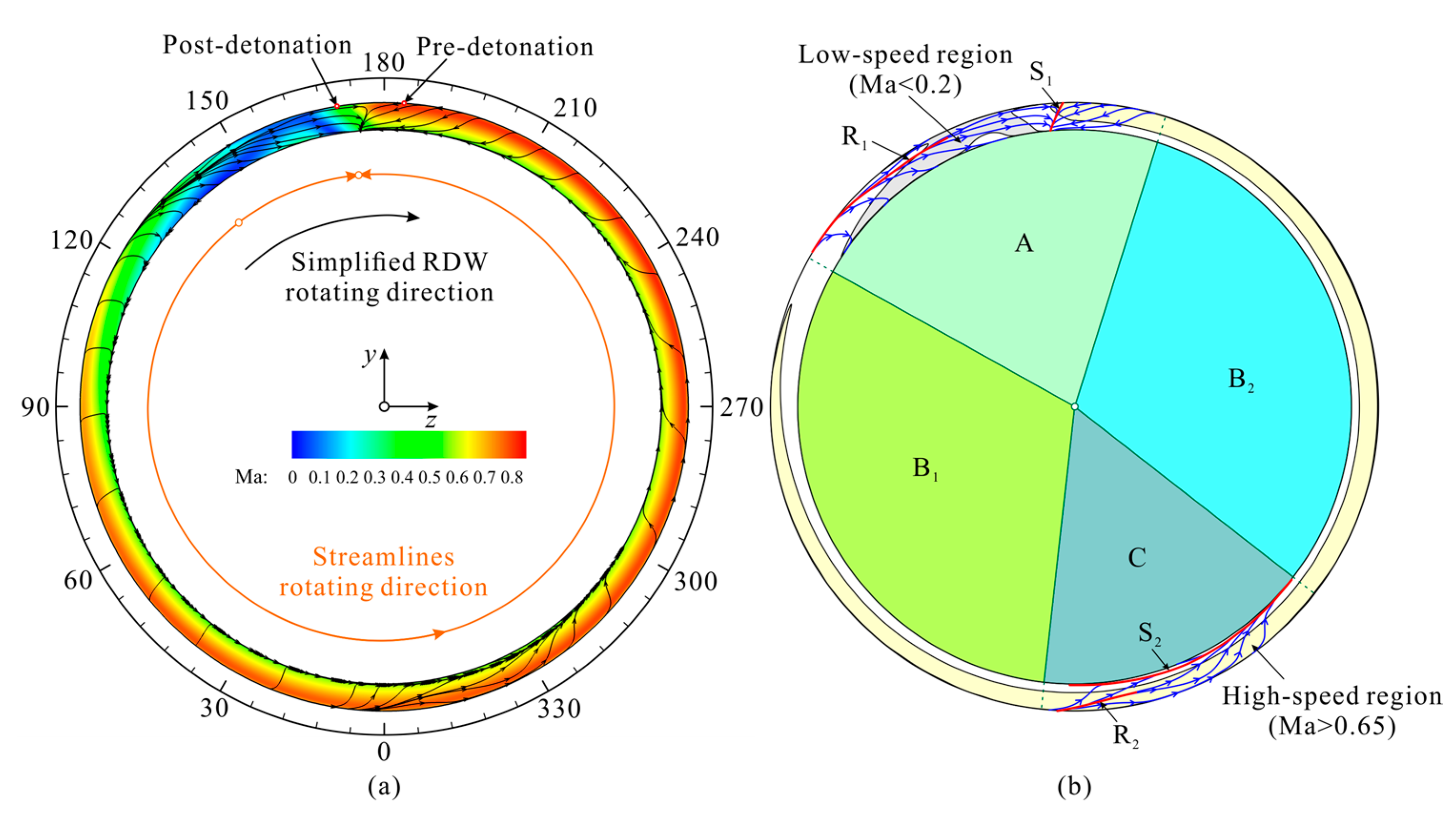
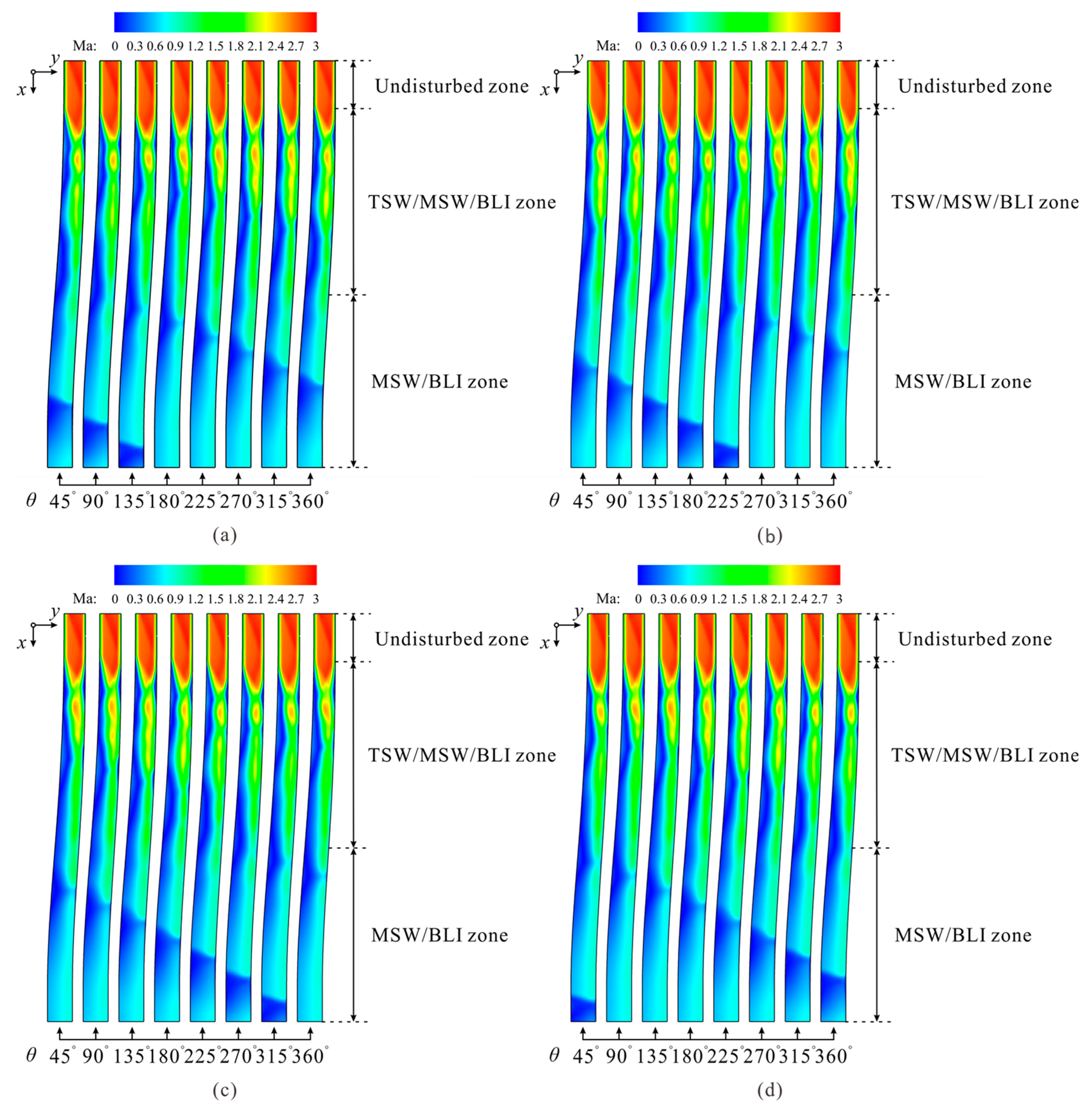
4.3. Flow Patterns at the Exit

Another important issue that should be discussed is the flow pattern at the exit, as presented in Figure 12. As can be seen, three types of zones are determined in Figure 12b, based on the morphology of the streamlines: zone A is referred to as the rotating detonation wave/boundary layer interaction (RDW/BLI) zone, zone B, consisting of B1 and B2, is dominated by the expansion waves, and zone C is where the helical vortices are exhausted from the isolator. Still, there are some generalities in the three zones. The radial velocity vr maintains a negative at every azimuthal angle θ, owing to the radial pressure gradient induced at the first bend of the “S-shaped” section. As a result of the radial pressure gradient, the low-speed flow accumulates in the minor-radius region, driving the high-speed flow to migrate to the major-radius one. In zone A, disturbed by the simplified RDW, the positive circumferential velocity vθ of the flow is induced after the RDW, that is, the streamlines point towards the RDW. Thus, a separation line S1 that is almost normal to the walls is formed under the strong adverse pressure gradient that originated from the RDW, then a reattachment line R1 that is nearly parallel to the outer wall could be noted in the angle range of 120°–150°, due to the expansion effects. A quasi-triangular gap in the low-speed region can be found near the inner wall, which is caused by the high-speed streamlines released from line R1. As a result, the low-speed region is shaped like a “Λ”. As for zone B, due to the expansion effect behind the MSW, vθ decreases to below 0 gradually, causing the flow to rotate counter-clockwise (the view direction is along the negative x-axis). It can be found that the twist of the streamlines in zone B2 is more violent than that in zone B1. In zone C, the vortices generated from the boundary layer near the inner wall exhaust into the RDC, as shown in Figure 9b, hence the streamlines here are perturbated, which contribute to the formation of the separation line S2 and the reattachment line R2.

5. Self-Similarity in the Isolator Affected by the Rotating Feedback Pressure

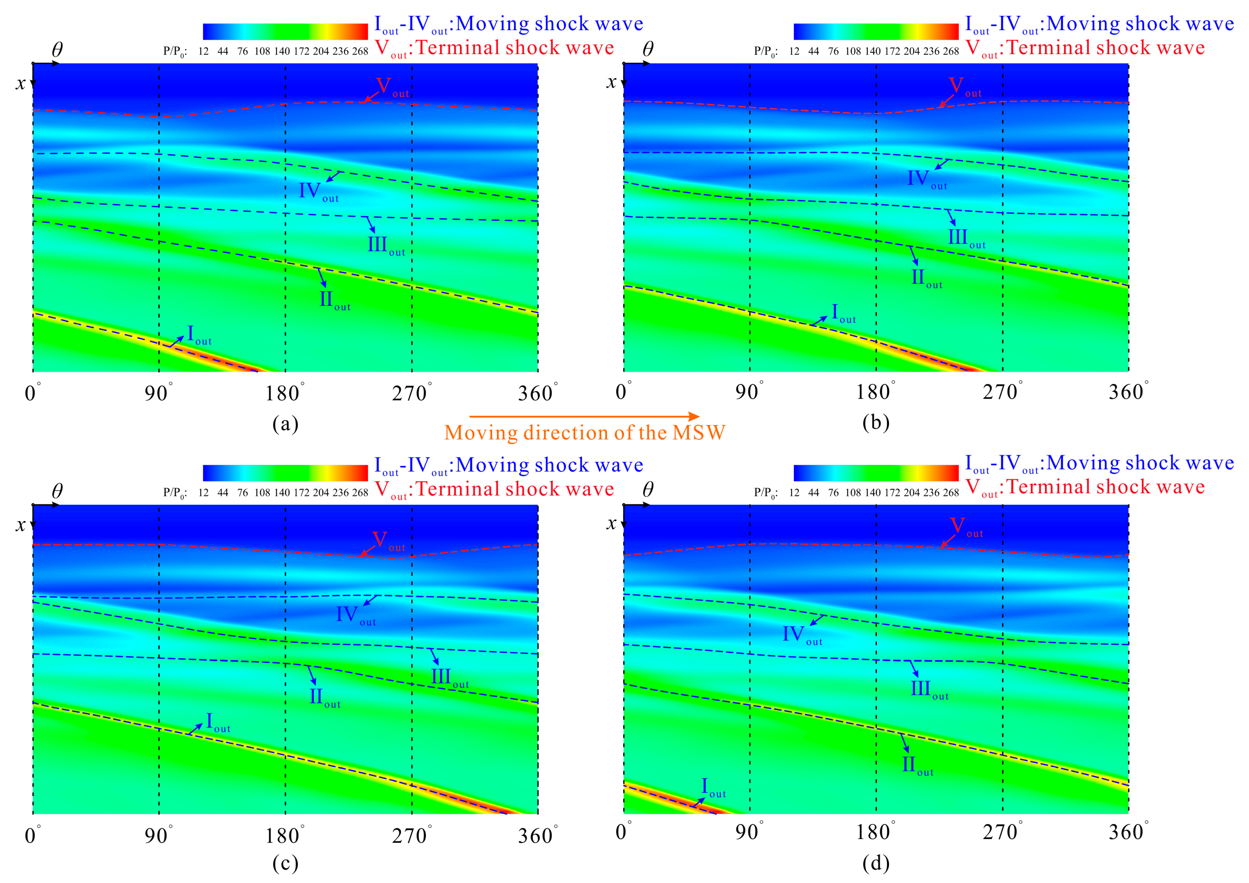
5.1. Similarity of the Flow Patterns between Adjacent Cycles

To demonstrate the correlations of the flow-field between two adjacent cycles, Figure 13 compares the wall pressure and the sectional Mach number contours in two neighbor cycles. An interesting discovery is that the pressure contour on the outer wall at t = nT and t = (n + 1)T are extremely similar, both consisting of four curved oblique MSWs with analogous patterns and comparative strength. As mentioned above, the flow-field of the meridian planes in Figure 13a,b could both be split into three zones, i.e., the undisturbed zone, the TSW/MSW/BLI zone, and the MSW/BLI zone. The distribution and shape of the low-momentum flow regions resemble each other, as well. Further, the flow patterns in the meridian planes situated on both sides of the RDW (θ = 135°, and θ = 225°) at t = nT and t = (n + 1)T are contrasted in Figure 14, which corresponds to points A1, B1, A2, B2 emphasized in Figure 15. As can be seen, the Mach number and wall pressure profiles of two meridian planes at t = nT are basically consistent with those at t = (n + 1)T, correspondingly. Thus, it can be deduced that the flow-field in the adjacent cycles are self-similar.

5.2. Comparison of the Flow Patterns at Different Moments in One Cycle

Then, the overall flow-fields at different moments in one cycle are compared in Figure 16 and Figure 17. It should be noted that the time difference among the selected four moments equals T/4, that is, the feedback pressure at the exit rotates a corresponding angle in sequence, which equals 360°/4 = 90° in this case. Hence, it is valid to assume that the isolator flow-field should also rotate 90°. Take the meridian plane with θ = 135° at t = nT corresponding to point A1 in Figure 18 as a reference plane, the comparison among the sectional flow patterns of A1 and that with θ = 135° + 90° = 225° at t = (n + 1/4)T (B2 in Figure 18), that with θ = 135° + 2∙90° = 315° at t = (n + 2/4)T (C2 in Figure 18) and that with θ = 135° + 3∙90° = 45° at t = (n + 3/4)T (D2 in Figure 18) is rather reasonable for the validation of flow-field similarity at different moments in one cycle.
Likewise, it can be discovered that the global flow structures of the isolator at different moments in one cycle all show good agreement, though the flow-field rotates 90°. The structure of the shock waves, the scale and distribution of the low-momentum flow, even the surface pressure change curves and the Mach number contours of the corresponding meridian planes exhibited in Figure 19 all match perfectly, which confirms the self-similarity of the isolator flow in one cycle under rotating Pb.
Based on the preceding discussions, we can draw the conclusion that the flow-field of the isolator under rotating feedback pressure perturbations is similar during the stable operating stage, which indicates that the rotation angular velocity of the TSW and the MSWs are equal and hold invariant, building the key foundation for the theoretical model of the inclination angle of the MSWs through velocity decomposition, previously mentioned in Section 6.

6. Theoretical Model of the Inclination Angles of the Moving Shock Wave, Based on Velocity Decomposition

The shock wave structure on the central plane of the isolator at t = nT, as shown in Figure 20, is chosen to calculate the inclination angle α of the MSWs. It can be discovered that the MSWs appear approximately as straight lines, indicating that the MSW angle α varies with little discrepancy in one round. Hence, the average parameters could be utilized to compute the inclination angle of each MSW separately. MSW i is taken as an example to introduce the theoretical model, the schematic of which is exhibited in Figure 21. The inclination angle of MSW i αi is defined as the inclination angle between MSW i and the axis. Since the absolute values of the radial and circumferential velocities of the pre-shock air are ignorable, compared with the pre-shock axial velocity according to Figure 10, it is valid to assume that the pre-shock air flows along the axis. So αi also refers to the inclination angle between MSW i and the pre-shock flow direction. In addition, there is a negative correlation between αi and βi, which is given as:
αi + βi = 90°,
The movement of MSW i between t = nT illustrated by the solid red line and t′ = nT + dt illustrated by the dashed red line could be deconstructed into two parts:
dxsi = vsi,adt,
dlsi = vsi,θdt,
where dxsi and dlsi denote the movement distance of MSW i in the axis direction and circumferential direction, respectively; vsi,a and vsi,θ denote the absolute velocity of MSW i in the axis direction and circumferential direction, separately.
In addition, MSW i at t = nT is parallel to that at t′ = nT + dt (dt → 0) due to the self-similarity property of the flow-field demonstrated in Section 5. Thus, αi also refers to the inclination angle between the axial velocity vsi,a and the resultant velocity vsi of MSW i, computed by:
v si = v si , θ v si , θ + v si , a v si , a
αi = atan(vsi,θ/vsi,a),
It is noteworthy that vsi refers to the absolute velocity of MSW i, and it is known that the angular velocity of the MSWs equals that of the simplified RDW, which is defined as:
ω = 2πf,
Hence,
vsi,θ = ωri,
vsi,a = vpi,avpre-i,a,
where vpre-i,a denotes the absolute velocity of the pre-shock air in the axial direction, which is defined by temperature Tpre-i and Mach number Mpre-i of the air before MSW i:
v pre - i , a = γ R T pre - i M pre - i
and vpi,a denotes the axial velocity of MSW i relative to the pre-shock flow, i.e., the axial propagation velocity of MSW i, which is the next key factor to be calculated.
The calculation method of vpi,a is illustrated in Figure 22. The sketch of MSW i and the absolute velocity of MSW i and the pre-shock air at t = nT is presented in Figure 22a. Firstly, a microelement of MSW i dssi is extracted, and the MSW i coordinate system is established, as shown in Figure 22b. On this basis, the relative velocity of the pre-shock air vpre-i,rel could be deconstructed into −vsi,θ in the circumferential direction and −vpi,a in the axial direction, and MSW i microelement dssi consists of dxsi and dlsi. Hence, αi could also be obtained by:
αi = atan(dlsi/dxsi),
Then, the relative velocity of the pre-shock air vpre-i,rel and MSW i microelement dssi are both axially and circumferentially deconstructed into four types shown in Figure 22c. Type (1) refers to the collision between the air with an axial velocity -vpi,a and the circumferential microelement of MSW i dlsi, type (2) exhibits the encounter between the air with a circumferential velocity -vsi,θ and MSW i circumferential microelement dlsi, while type (3) and (4) indicate the meeting of MSW i axial microelement dxsi and the air with the axial (−vpi,a) and circumferential (−vsi,θ) velocity, successively.
It can be discovered that only type (1) is relevant with the calculation of vpi,a, since the components of the pre-shock relative velocity are both parallel to the components of MSW i microelement in type (2) and (3), which will not induce a pressure rise; though the circumferential component of the pre-shock relative velocity −vsi,θ is perpendicular to the axial component of MSW i microelement dxsi in type (4), there is no correlation between the circumferential pressure rise induced and vpi,a. Hence, the functions of vpi,a and ΔPa are as follows:
M pi , a = γ + 1 2 γ ( P post - i P pre - i ) a + γ 1 2 γ
( P post - i P pre - i ) a = P pre - i + Δ P a P pre - i
v pi , a = γ R T pre - i M pi , a
where ΔPa denotes the axial component of the pressure gradient originating from MSW i, and Mpi,a denotes the axial propagation Mach number of MSW i.
Last, the integral average calculation along MSW i is performed, and MSW i angle αi computed by Equations (11) and (16) are compared, as shown in Table 4, along with those of MSW ii and iii. To distinguish from each other, the α ¯ calculated by Equation (11) is referred to as the predicted angle α ¯ aero , and the inclination angle obtained via Equation (16) is defined as the measured angle α ¯ geom . The relative error δα is defined as:
δ α = ( α ¯ aero α ¯ geom ) α ¯ geom × 100 %
As can be seen, the absolute value of the relative errors of the inclination angles are below 3%, indicating that the theoretical method based on the velocity decomposition on the MSW angles α is reasonable, with a proper accuracy and feasibility. Moreover, the predicted results give a clear and sensible explanation of the physical meaning of the MSW angles and the propagation of the MSWs, which provides some guidance to further investigations on the isolator with the simplified RDW under complex boundary conditions and with the real RDW.

7. Conclusions

Herein, the three-dimensional simulations on an annular isolator under rotating feedback pressure perturbations simplified from the single-mode rotating denotation wave (RDW), which is modeled as a periodical function consists of two linear variation zones and one curve change zone given by a transformed trigonometric function, are performed. The transient flow characteristics dominated by the moving shock wave/boundary layer interaction (MSW/BLI) is investigated thoroughly, and the self-similarity property of the flow-field is evaluated. Furthermore, the theoretical model of the inclination angle of the moving shock wave (MSW) by velocity decomposition is developed and validated.
It is found that a helical MSW and a terminal shock wave (TSW) are generated in the isolator due to the upstream and circumferential propagation of the feedback pressure perturbations. As a result, the flow-fields could be divided into three regions, i.e., the undisturbed zone, the terminal shock wave/moving shock wave/boundary layer interaction (TSW/MSW/BLI) zone, and the MSW/BLI zone. In the TSW/MSW/BLI zone, the rather small axial distance between the TSW and the MSW connects the two adverse-pressure gradients induced by the shocks, intensifying the flow separation on the meridian planes with smaller azimuthal angles, which rolls up vortices in the vicinity of the outer and inner walls. These vortices all develop along the TSW and the MSWs, presenting a typical glancing shock wave/boundary layer interaction (GSW/BLI). As a result, the migration of the separation bubbles makes the separation scale on the meridian plane at θ = 180° the maximum. In the MSW/BLI zone, the shock induces the boundary layer to separate, forming a helical vortex located at the foot of the MSW. During the upstream propagation process, the pattern of the MSWs transforms from a moving normal shock wave to a moving oblique shock wave with decreased strength, the screw-pitch of the MSW reduces slightly, and the inclination angle of the MSW increases gently. In other words, the MSW shows more “flat” patterns along the negative direction of the x-axis. Furthermore, the TSW shows some characteristics of a standing shock wave, causing the static pressure, temperature, and entropy of the flow to increase instantly and the velocity to drop in three directions. Whereafter, following the collisions with MSW, the static pressure, temperature, entropy, and circumferential velocity of the air rise instantly, while the axial velocity drops to a lower level. It is interesting to find that though the MSW do deflect the streamlines, the air still maintains an axial flow at the exit except in the adjacent region of the MSW with the neglected radial velocity and circumferential velocity. Likewise, three types of zones can be determined in the flow pattern at the exit: the rotating detonation wave/boundary layer interaction (RDW/BLI) zone, the expansion zone, and the vortices discharge zone.
Then, the self-similarity property is observed in the flow-field of the annular isolator under rotating feedback pressure perturbations, which connects the transient flow patterns at different moments with each other. The global flow structure of the isolator at different moments all show good agreement despite its rotation with the RDW, and the surface pressure profiles of the corresponding meridian plane all match perfectly. Such a characteristic indicates that the rotation angular velocity of the TSW and the MSW are equal and hold invariant, and the isolator flow could be regarded as a quasi-steady flow, i.e., independence of time. On this basis, the theoretical model of the MSW angles by coordinate transformation and velocity decomposition is introduced and validated. This model establishes contacts between the geometric form and the velocity triangle of the MSW for the first time, the latter of which is determined by its variation period and the original axial pressure gradient. The relative errors between the predicted and the geometrical results are below 3%, which confirms the reasonability and preciseness of the theoretical model, offering a rapid method to predict the shape of the MSW, and a perspective to better understand the physical meaning of the shape of the MSW.

Author Contributions

Conceptualization, Z.L.; methodology, H.H. and H.T.; validation, Z.L., H.H. and H.T.; formal analysis, Z.L.; investigation, Z.L.; resources, H.H.; data curation, H.H. and H.T.; writing—original draft preparation, Z.L.; writing—review and editing, H.H., H.T., G.L.; visualization, J.L.; supervision, H.H. and H.T.; project administration, Y.W.; funding acquisition, L.L. All authors have read and agreed to the published version of the manuscript.

Funding

This work was funded by the National Natural Science Foundation of China (Grant Nos. 12272177, 51906104, and U20A2070), the National Science and Technology Major Project (No. J2019-II-0014-0035), 1912 Project (No. 2019-JCJQ-DA001-164), the Foundation of National Key Laboratory of Transient Physics (No.6142604200212), and the priority academic program development of Jiangsu higher education institutions.

Institutional Review Board Statement

Not applicable.

Data Availability Statement

The data within the article will be available upon request.

Conflicts of Interest

The authors declare that they have no known competing financial interest or personal relationships that could have appeared to influence the work reported in this paper.

References

  1. Lu, F.K.; Braun, E.M. Rotating detonation wave propulsion: Experimental challenges, modeling, and engine concepts. J. Propul. Power 2014, 30, 1125–1142. [Google Scholar] [CrossRef] [Green Version]
  2. Wolanski, P. Detonative propulsion. Proc. Combust. Inst. 2013, 34, 125–158. [Google Scholar] [CrossRef]
  3. Anand, V.; Gutmark, E. Rotating detonation combustors and their similarities to rocket instabilities. Prog. Energy Combust. Sci. 2019, 73, 182–234. [Google Scholar] [CrossRef] [Green Version]
  4. Rong, G.; Cheng, M.; Sheng, Z.-H.; Liu, X.-Y.; Zhang, Y.-Z.; Wang, J.-P. Investigation of counter-rotating shock wave and wave direction control of hollow rotating detonation engine with Laval nozzle. Phys. Fluids 2022, 34, 056104. [Google Scholar] [CrossRef]
  5. Hexia, H.; Huijun, T.; Wang, J.; Le Ning, S.S. A fluidic control method of shock train in hypersonic inlet/isolator. In Proceedings of the 50th AIAA/ASME/SAE/ASEE Joint Propulsion Conference, Cleveland, OH, USA, 28–30 July 2014. [Google Scholar]
  6. Matsuo, K.; Miyazato, Y.; Kim, H.D. Shock train and pseudo-shock phenomena in internal gas flows. Prog. Aerosp. Sci. 1999, 35, 33–100. [Google Scholar] [CrossRef]
  7. Bykovskii, F.A.; Zhdan, S.A.; Vedernikov, E.F. Continuous spin detonations. J. Propul. Power 2006, 22, 1204–1216. [Google Scholar] [CrossRef]
  8. Voitsekhovskii, B. Stationary spin detonation. Sov. J. Appl. Mech. Tech. Phys. 1960, 3, 157–164. [Google Scholar]
  9. Zhdan, S.A. Mathematical model of continuous detonation in an annular combustor with a supersonic flow velocity. Combust. Explos. Shock Waves 2008, 44, 690–697. [Google Scholar] [CrossRef]
  10. Zhu, W.; Wang, Y.; Wang, J. Flow field of a rotating detonation engine fueled by carbon. Phys. Fluids 2022, 34, 073311. [Google Scholar] [CrossRef]
  11. Uemura, Y.; Hayashi, A.K.; Asahara, M.; Tsuboi, N.; Yamada, E. Transverse wave generation mechanism in rotating detonation. Proc. Combust. Inst. 2013, 34, 1981–1989. [Google Scholar] [CrossRef]
  12. Zhou, R.; Wang, J.P. Numerical investigation of flow particle paths and thermodynamic performance of continuously rotating detonation engines. Combust. Flame 2012, 159, 3632–3645. [Google Scholar] [CrossRef]
  13. Smirnov, N.; Nikitin, V.; Stamov, L.; Mikhalchenko, E.; Tyurenkova, V. Rotating detonation in a ramjet engine three-dimensional modeling. Aero. Sci. Technol. 2018, 81, 213–224. [Google Scholar] [CrossRef]
  14. Smirnov, N.; Nikitin, V.; Stamov, L.; Mikhalchenko, E.; Tyurenkova, V. Three-dimensional modeling of rotating detonation in a ramjet engine. Acta Astronaut. 2019, 163, 168–176. [Google Scholar] [CrossRef]
  15. Liu, S.-J.; Lin, Z.-Y.; Liu, W.-D.; Lin, W.; Zhuang, F.-C. Experimental realization of H2/air continuous rotating detonation in a cylindrical combustor. Combust. Sci. Technol. 2012, 184, 1302–1317. [Google Scholar] [CrossRef]
  16. Lin, W.; Zhou, J.; Liu, S.; Lin, Z.; Zhuang, F. Experimental study on propagation mode of H2/Air continuously rotating detonation wave. Int. J. Hydrogen Energy 2015, 40, 1980–1993. [Google Scholar] [CrossRef]
  17. Wang, C.; Liu, W.; Liu, S.; Jiang, L.; Lin, Z. Experimental investigation on detonation combustion patterns of hydrogen/vitiated air with annular combustor. Exp. Therm Fluid Sci. 2015, 66, 269–278. [Google Scholar] [CrossRef]
  18. Bluemner, R.; Bohon, M.; Paschereit, C.; Gutmark, E. Counter-rotating wave mode transition dynamics in an RDC. Int. J. Hydrogen Energy 2019, 44, 7628–7641. [Google Scholar] [CrossRef]
  19. Han, J.; Bai, Q.; Zhang, S.; Weng, C. Experimental study on propagation mode of rotating detonation wave with cracked kerosene gas and ambient temperature air. Phys. Fluids 2022, 34, 075127. [Google Scholar] [CrossRef]
  20. Naples, J.; Hoke, J.; Karnesky; Schauer, F. Flowfield Characterization of a Rotating Detonation Engine. In Proceedings of the 51st AIAA Aerospace Sciences Meeting Including the New Horizons Forum and Aerospace Exposition, Dallas, TX, USA, 7–10 January 2013. [Google Scholar]
  21. Anand, V.; George, A.S.; Driscoll, R.; Gutmark, E. Characterization of instabilities in a rotating detonation combustor. Int. J. Hydrogen Energy 2015, 40, 16649–16659. [Google Scholar] [CrossRef]
  22. Liu, Y.S.; Wang, Y.H.; Li, Y.S.; Li, Y.; Wang, J.P. Spectral analysis and self-adjusting mechanism for oscillation phenomenon in H2/O2 continuously rotating detonation engine. Chin. J. Aeronaut. 2015, 28, 669–675. [Google Scholar] [CrossRef] [Green Version]
  23. Wu, Y.X.; Ma, H.; Peng, L.; Gao, J. Experimental research on initiation characteristics of a rotating detonation engine. Exp. Therm. Fluid Sci. 2016, 71, 154–163. [Google Scholar]
  24. Liu, Y.; Zhou, W.; Yang, Y.; Liu, Z.; Wang, J. Numerical study on the instabilities in H2-air rotating detonation engines. Phys. Fluids 2018, 30, 046106. [Google Scholar] [CrossRef]
  25. Schwer, D.; Kailasanath, K. Effect of Inlet on Fill Region and Performance of Rotating Detonation Engines. In Proceedings of the 47th AIAA/ASME/SAE/ASEE Joint Propulsion Conference & Exhibit, San Diego, CA, USA, 31 July–3 August 2011. [Google Scholar]
  26. Anand, V.; St George, A.; Driscoll, R.; Gutmark, E. Analysis of air inlet and fuel plenum behavior in a rotating detonation combustor. Exp. Therm. Fluid Sci. 2016, 70, 408–416. [Google Scholar] [CrossRef]
  27. Schwer, D.A.; Kailasanath, K.; Kaemming, T. Pressure characteristics of a ram-RDE diffuser. Aerosp. Sci. Technol. 2019, 85, 187–198. [Google Scholar] [CrossRef]
  28. Frolov, S.M.; Dubrovskii, A.V.; Ivanov, V.S. Three-dimensional numerical simulation of operation process in rotating detonation engine. Prog. Propuls. Phys. 2013, 4, 467–488. [Google Scholar]
  29. Frolov, S.M.; Dubrovsky, A.V.; Ivanov, V.S. Three-Dimensional Numerical Simulation of a Continuously Rotating Detonation in the Annular Combustion Chamber with a Wide Gap and Separate Delivery of Fuel and Oxidizer. In Proceedings of the 5th EUCASS, Munich, Germany, 1–6 July 2013. [Google Scholar]
  30. Dyson, R.W. Flow Diode and Method for Controlling Fluid Flow Origin of the Invention. US Patent 9169855 B1, 4 November 2015. [Google Scholar]
  31. Liu, S.; Liu, W.; Jiang, L.; Lin, Z. Numerical investigation on the airbreathing continuous rotating detonation engine. In Proceedings of the 25th ICDERS, Leeds (ICDERS, 2015), Leeds, UK, 2–7 August 2015; Volume 157. [Google Scholar]
  32. Wang, G.; Liu, W.; Liu, S.; Zhang, H.; Peng, H.; Zhou, Y. Experimental verification of cylindrical air-breathing continuous rotating detonation engine fueled by non-premixed ethylene. Acta Astronaut. 2021, 189, 722–732. [Google Scholar] [CrossRef]
  33. Dubrovskii, V.; Ivanov, A.; Zangiev; Frolov, S. Three-dimensional numerical simulation of the characteristics of a ramjet power plant with a continuous-detonation combustor in supersonic flight. Russ. J. Phys. Chem. B 2016, 10, 469–482. [Google Scholar] [CrossRef]
  34. Mengmeng, Z.; Buttsworth, D.; Gollan, R.; Jacobs, P. Simulation of a Rotating Detonation Ramjet Model in Mach 4 Flow. Simulation 2018, 10, 1321. [Google Scholar]
  35. Wu, K.; Zhang, S.; Luan, M.; Wang, J. Effects of flow-field structures on the stability of rotating detonation ramjet engine. Acta Astronaut. 2020, 168, 174–181. [Google Scholar] [CrossRef]
  36. Wu, K.; Zhang, S.; Shen, D.; Wang, J. Analysis of flow-field characteristics and pressure gain in air-breathing rotating detonation combustor. Phys. Fluids 2021, 33, 126112. [Google Scholar] [CrossRef]
  37. Menter, F.R. Two-equation eddy-viscosity turbulence models for engineering applications. AIAA J. 1994, 32, 1598–1605. [Google Scholar] [CrossRef] [Green Version]
  38. Jianhua, C. Backpressure Characteristics of Annular Isolator in CRDR; National University of Defense Technology: Changsha, China, 2017. [Google Scholar]
  39. Yue, S. Numerical Research on the Effects of Ramjet Rotating Detonation on the Incoming Flow; National University of Defense Technology: Changsha, China, 2019. [Google Scholar]
  40. Peng, H.Y.; Liu, W.D.; Liu, S.J.; Zhang, H.L. Experimental investigations on ethylene-air continuous rotating detonation wave in the hollow chamber with laval nozzle. Acta Astronaut. 2018, 151, 137–145. [Google Scholar] [CrossRef]
  41. Peng, H.-Y.; Liu, W.-D.; Liu, S.-J.; Zhang, H.-L.; Jiang, L.-X. Flowfield analysis and reconstruction of ethylene–air continuous rotating detonation wave. AIAA J. 2020, 58, 5036–5045. [Google Scholar] [CrossRef]
  42. Rentao, Z. Study of Flow Characteristics of Rotating Detonation Engine Inlet; Nanjing University of Aeronautics and Astronautics: Changsha, China, 2019. [Google Scholar]
  43. Igra, O.; Wang, L.; Palcovitz, J.; Heilig, W. Shock wave propagation in a branched duct. Shock Waves 1998, 8, 375–381. [Google Scholar] [CrossRef]
  44. Mazor, G.; Igra, O.; Ben-Dor, G.; Mond, M.; Reichenbach, H.; Smith, F.T. Head-on collision of normal shock waves with a rubber-supported wall. Philos. Trans. R. Soc. Lond. Ser. A Phys. Eng. Sci. 1992, 338, 237–269. [Google Scholar] [CrossRef]
  45. Chao, W. Self-Sustaining and Propagation Mechanism of Airbreathing Continuous Rotating Detonation Wave; National University of Defense Technology: Changsha, China, 2016. [Google Scholar]
  46. Yuan, H.; Liu, F.; Wang, X.; Zhou, Z. Design and analysis of a supersonic axisymmetric inlet based on controllable bleed slots. Aerosp. Sci. Technol. 2021, 118, 107008. [Google Scholar] [CrossRef]
  47. Liu, J.; Liu, C. Modified normalized Rortex/vortex identification method. Phys. Fluids 2019, 31, 061704. [Google Scholar] [CrossRef] [Green Version]
  48. Dong, X.; Gao, Y.; Liu, C. New normalized Rortex/vortex identification method. Phys. Fluids 2019, 31, 011701. [Google Scholar] [CrossRef]
  49. Kalkhoran, M.; Smart, M.K. Aspects of shock wave-induced vortex breakdown. Prog. Aerosp. Sci. 2000, 36, 63–95. [Google Scholar] [CrossRef]
  50. Liang, G.; Huang, H.; Tan, H.; Luo, Z.; Tang, X.; Li, C.; Cai, J. Shock train/glancing shock/boundary layer interaction in a curved isolator with sidewall contraction. Phys. Fluids 2022, 34, 116106. [Google Scholar] [CrossRef]
Figure 1. Sketch of the isolator model.
Aerospace 10 00188 g001
Figure 2. Surface grid and boundary conditions. (a) Surface grid. (b) Computational domain and boundary conditions.
Aerospace 10 00188 g002
Figure 3. Spatial and temporal distribution of the feedback pressure. (a) Static pressure contour at the exit when t satisfies the equation floor (t, T) = 0. (b) The curve of the feedback pressure with time in a cycle, where Pb in section a-b, b-c and c-d is calculated by Equations (3)–(5), successively.
Aerospace 10 00188 g003
Figure 4. Comparison of between the numerical (top) and experimental (bottom) schlieren images. (a) t = 28 μs. (b) t = 40.5 μs.
Aerospace 10 00188 g004
Figure 5. Comparison of the computed outer-wall pressure distribution for the three grid densities.
Aerospace 10 00188 g005
Figure 6. Shock wave structures. (a) Pressure contour on the outer wall after the coordinate change. (b) Pressure contour on the inner wall after the coordinate change. (c) Three-dimensional schematic diagram of the moving shock wave and the terminal shock wave.
Aerospace 10 00188 g006
Figure 7. Flow patterns on eight meridian planes of different angles. (a) Mach number contours. (b) Pressure contours.
Aerospace 10 00188 g007
Figure 8. Surface pressure distributions and secondary flow structure on the meridian plane at θ = 135°.
Aerospace 10 00188 g008
Figure 9. Vortex structures originate. (a) Three-dimensional streamlines released from the entrance at eight angles without the vicinity of the inner surface. (b) Three-dimensional streamlines released from the entrance at eight angles without the vicinity of the outer surface. (c) Three-dimensional vortices and the inner-wall pressure contour.
Aerospace 10 00188 g009
Figure 10. Aerodynamic parameter distribution curves of the sectional centerlines along the axial direction. (a) θ = 135°. (b) θ = 180°.
Aerospace 10 00188 g010
Figure 11. Entropy profile of the sectional centerlines along the axial direction. (a) θ = 135°. (b) θ = 180°.
Aerospace 10 00188 g011
Figure 12. Flow topology on the exit. (a) Absolute Mach number contour and the streamlines. (b) Sketch of the distilled flow structure.
Aerospace 10 00188 g012
Figure 13. Critical flow structure in the adjacent cycles. (a) Pressure contour on the outer wall, t = nT. (b) Pressure contour on the outer wall, t = (n + 1)T. (c) Mach number contour of eight meridian planes, t = nT. (d) Mach number contour of eight meridian planes, t = (n + 1)T.
Aerospace 10 00188 g013
Figure 14. Comparison of the Mach number and pressure profiles of the meridian planes in adjacent cycles. (a) θ = 135°. (b) θ = 225°.
Aerospace 10 00188 g014
Figure 15. Feedback pressure change curve with time, where points A1 and A2 denote the meridian plane with θ = 135° at t = nT and t = (n + 1)T, respectively, and points B1 and B2 denote the meridian plane with θ = 225° at t = nT and t = (n + 1)T, respectively.
Aerospace 10 00188 g015
Figure 16. Pressure contours on the outer wall at different moments in one period. (a) t = nT. (b) t = (n + 1/4)T. (c) t = (n + 2/4)T. (d) t = (n + 3/4)T.
Aerospace 10 00188 g016
Figure 17. Mach number contours of eight meridian planes at different moments in one period. (a) t = nT. (b) t = (n + 1/4)T. (c) t = (n + 2/4)T. (d) t = (n + 3/4)T.
Aerospace 10 00188 g017
Figure 18. Feedback pressure change curve with time, where points A1, B1, C1, and D1 denote the meridian plane with θ = 135°, 225°, 315°, and 45° at t = nT successively, point B2 denotes that with θ = 225° at t = (n + 0.25)T, point C2 denotes that with θ = 315° at t = (n + 0.5)T, and point D2 denotes that with θ = 45° at t = (n + 0.75)T.
Aerospace 10 00188 g018
Figure 19. Mach number and pressure profiles of corresponding meridian planes at different moments in one period.
Aerospace 10 00188 g019
Figure 20. Shock wave structure on the central plane at t = nT in x-l plane, where l denotes the arc length, and the dependent ratio of x and l equals 1.
Aerospace 10 00188 g020
Figure 21. Sketch of MSW i.
Aerospace 10 00188 g021
Figure 22. Sketch of the calculation method. (a) MSW i and the absolute velocity of air and MSW i. (b) the MSW i microelement and the relative velocity of air. (c) Components of the relative velocity and MSW i. (d) Relevant component with vpi,a.
Aerospace 10 00188 g022
Table 1. Geometric parameters of the isolator.
ParameterValue
Liso, mm228.43
LS-shaped, mm208.43
Rent-in, mm152.28
Hent, mm12.00
Rexi-in, mm143.00
Hexi, mm14.00
Roff,iso, mm8.28
Table 2. Incoming flow conditions at the entrance.
ParameterValue
Mean Mach number Ment2.67
Total pressure Pt,ent, kPa1423.07
Static pressure Pent18.94 P0
Static temperature Tent, K554.45
Nominal boundary layer thickness δent, mm1.09
Table 3. Main parameters of Pb.
ParameterValue
Peak value280 P0
Valley value104.6 P0
Variation period T, s2 × 10−4
Variation frequency f, Hz5000
Table 4. Integral average results of the MSWs.
ParametersValue
MSW iMSW iiMSWb iii
v ¯ si , a , m/s657.50485.44−3.75
v ¯ si , θ , m/s4716.844797.934932.15
α ¯ aero , °82.0784.2290.04
α ¯ geom , °83.9485.9987.77
δα, %−2.23−2.062.58
Disclaimer/Publisher’s Note: The statements, opinions and data contained in all publications are solely those of the individual author(s) and contributor(s) and not of MDPI and/or the editor(s). MDPI and/or the editor(s) disclaim responsibility for any injury to people or property resulting from any ideas, methods, instructions or products referred to in the content.

