Article

Predictive Model of a Mole-Type Burrowing Robot for Lunar Subsurface Exploration

1
School of Aeronautics and Astronautics, University of Chinese Academy of Sciences, Beijing 100039, China
2
Key Laboratory of Space Utilization, Technology and Engineering Center for Space Utilization, Chinese Academy of Sciences, Beijing 100094, China
*
Author to whom correspondence should be addressed.
Aerospace 2023, 10(2), 190; https://doi.org/10.3390/aerospace10020190
Submission received: 30 November 2022 / Revised: 10 February 2023 / Accepted: 14 February 2023 / Published: 16 February 2023
(This article belongs to the Section Astronautics & Space Science)

Abstract

:
In this work, a dynamic model is proposed to simulate the drilling and steering process of an autonomous burrowing mole to access scientific samples from the deep subsurface of the Moon. The locomotive module is idealized as a rigid rod. The characteristic parameters are considered, including the length, cross-section diameter, and centroid of a cylindrical rod. Based on classical Lagrangian mechanics, a 3-DOF dynamic model for the locomotion of this autonomous device is developed. By introducing resistive force theory, the interaction scheme between the locomotive body and the lunar regolith is described. The effects of characteristic parameters on resistive forces and torques are studied and discussed. Proportional-derivative control strategies are introduced to calculate the tracking control forces following a planned trajectory. The simulation results show that this method provides a reliable manipulation of a mole-type robot to avoid obstacles during the tracking control process in layered sediments. Overall, the proposed reduced-order model is able to simulate the operating and controlling scenarios of an autonomous burrowing robot in lunar subsurface environments. This model provides intuitive inputs to plan the space missions of a drilling robot to extract subsurface samples on an extraterrestrial planet such as the Moon or Mars.

1. Introduction

Extraterrestrial subsurface drilling and sampling is the core of near-Earth exploration missions, including the Moon, Mars, asteroids, etc. [1,2,3]. Typically, the surface of an extraterrestrial planet, such as the Moon, is covered by regolith, which consists of dust, fine granular particles, and agglutinates along the depth direction [4,5]. For scientific purposes, it is necessary to reach the subsurface destination and obtain geology samples with high scientific values [6]. Subsurface exploration equipment, including coring machines or robots, are the primary tools for providing insights into the evolutionary history of the solar system [2,7].
In recent space science projects, the concepts of underground mole-like robots or probes have been proposed [8,9]. For example, InSight’s HP3-Mole has been deployed to measure the internal heat flow of Mars [10]. This type of autonomous burrowing device is able to dive or steer itself to reach the desired target at suitable depths with tethered or autonomous communication. It might be a low-cost and high-efficient solution for a future space mission on the Moon or Mars [11]. Previous research has focused on the bio-inspired locomotion of animals or insects and developed robots that crawl, swim, and burrow [12,13] in fluid-like granular medium by mimicking the mechanisms of inchworms, earthworms, wood wasps, or gophers. For example, the inchworm robots, such as IDDS (Inchworm Deep Drilling System of NASA/Honeybee) [14] and IBR (Inchworm Boring Robot of CAST) [15], operate in a set of sequential actions of anchoring and drilling, in the same manner as worms. The wood wasp robots [16] simulate a reciprocating motion of two halves with backwards-facing teeth to shear and dig into the soil. The auto-gopher [17], a wireline drilling system, removes fragments discontinuously by running in a hole and conducting the coring operation repeatedly [18]. However, these technologies are all designed to penetrate along the orientation of robot bodies, without steering capacity. This capacity enables directional drilling and is a major enhancement of the existing drilling or coring methods. Although some conceptual designs and prototypes for lunar subsurface exploration have been developed, the locomotion in granular medium is still a challenging subject, and it remains a problem that requires investigation [1,7].
During the drilling process, resistive force is produced along the interaction between the robotic body and granular substances. Constructing a mathematical model of underground locomotion is the key to analyzing and maneuvering the robots in the downhole. There are several approaches to deal with such complex interactions between drilling robots and soils. For example, to treat the regolith as a fluid-like medium, the locomotion in the regolith can be modeled as a swimming movement at low Reynolds numbers [19,20]. The interaction between the intruder and the media is phenomenologically described by the hydrostatic pressure and fluid viscosity. However, the complexity of flow behaviors under different conditions are difficult to define via a unified form and group of parameters. Therefore, the regolith is most commonly viewed as granular particles. The empirical Resistive Force Theory (RFT) [21] and modified Archimedes’ Law Theory (MALT) [22] have been introduced to estimate the forces on objects moving at a constant speed within the particles of sand or soils. Considering the hydrostatic and viscosity terms of RFT, this calculation relies on the experimental calibration of specific parameters, while the treatments of both fluid mechanics and granular mechanics are sensitive to the geometry and penetrating velocity of intruder as well as the physical properties of regolith or soils [23].
Among numerical schemes, the Discrete Element Method (DEM) [24] is the widely used method to solve the kinematics of granular particles with sufficient microscopic details [25]. Kawamoto et al. [26] used DEM to simulate the macroscopic behaviors of granular materials influenced by particle shapes. Khademian et al. [27] simulated the mechanical behaviors of irregularly shaped lunar soils under triaxial tests. In the context of continuum mechanics, the Finite Element Method (FEM) resorts to the mathematical equation of contact behaviors to model the soil–tool interaction. Askari and Kamrin [28] used FEM to simulate the parametric geometries of an intruder moving in a granular media and revealed that the frictional yielding is the dominant factor in producing the resistive force in cohesionless media. However, to model the process of locomotion requires characterization of the complex constitutive properties or suitable criterions in order to describe the behaviors of granular matter, including nonlinearity, history-dependence, and nonlocality [29]. Thus, to model the locomotion in such “flowable” terrestrial materials is crucially depended on the invention of ingenious and complex constitutive equations, which is still an open problem in the literature [12,29,30].
For theoretical research and engineering application, some problems are solved and investigated via the simplified model, which is often used to describe the actual physical phenomenon. Winkler et al. [31] and Pasternak et al. [32] developed the classical models of a beam on an elastic foundation to solve the problems in the civil engineering field. In these models, soil–beam interaction is proposed mathematically, represented by a set of linear springs. Richard and Detournay et al. [33,34] built a dynamic model of rotational drill strings. In this dynamic model, drill strings are treated as an elastic beam, and the contact of drill strings and soil are described by linear or torsional springs, which represents the effects of weight on bit and torque, respectively. This method is also widely used in solving structure-oriented or dynamics-oriented problems [35,36].
In general, for a steerable burrowing robot, the drilling unit contains two major modules: excavating module to make an axial locomotion and steering module to make a deflection in the granular medium, respectively. To model this robot with sufficient details by a three-dimensional (3D) multi-physical FEM or DEM is very time-consuming. Therefore, to develop a simplified model is highly demanded in order to accelerate the development of steerable robots for the subsurface exploration of planetary bodies. In practice, the prediction of drilling forces and torques are strongly demanded in order to facilitate the robotic design and the development of a navigation algorithm. A reduced-order model is a practical way to model this complicated drilling device. This is beneficial in both the early design phase as a trade-off study toolbox and in the mission decision-making stage as a core in building a physics-based digital twin [37,38].
In this work, a rigid body dynamics model is proposed to simulate the operating and controlling scenarios of an autonomous robot steering in the lunar subsurface. The mole-type burrowing robot is idealized as a rigid intruder steering in the granular block with thick stacks of sediments, which represents the stratigraphic profiles of the geological structures of the Moon. The robotic locomotion is described by a 3-DOF rigid rod based on Lagrangian mechanics. The interaction between the locomotive body and lunar regolith is mathematically described as a contact model with both normal and shear stiffnesses. The effect of characteristic parameters on resistive forces and torques is studied and discussed through numerical experiments. To estimate the requirements of axial and lateral thrust by trajectory tracking, proportional-derivate (PD) control strategies are introduced and implemented into the dynamic equations.
The structure of the paper is organized as follows: first, the simplified model of a mole-type burrowing robot is introduced, and the proposed reduced-order model of locomotion is described. The numerical procedures are discussed for different parameters, including the driving forces, gravity, and time stepping, etc. Then, the dynamic behaviors of robotic locomotion are simulated and discussed via numerical experiments. Finally, its steerability and stability in the layered formations with PD control are discussed in detail.

2. Modeling Methods

The lunar subsurface within about 10 m in depth [39] consists of igneous regolith and disturbed materials from diverse causes, such as magmatic evolution, ejection blankets, and meteorite impacts [40,41]. The regolith or fragmental breccia consists of dust, fine granular particles, medium sized agglutinates, and bulky rocks along the horizontal direction. In addition, it contains a large number of basaltic rocks. Considering the internal geological surfaces formed by sedimented layers in a 3D lunar terrain domain [42], the steering locomotion to overcome distributed obstacles and hard formations is highly demanding for drilling and exploration in the lunar subsurface. For navigation purposes, the specified trajectory can be generated by subsurface imaging techniques using lunar penetrating radar (LPR) [43].
Therefore, the locomotion of an autonomous burrowing robot in the lunar regolith is designed to steer away from obstacles. Self-burrowing locomotion needs two fundamental mechanisms: the excavating unit creates the penetration and the steering unit controls the burrowing direction by adjusting the extension of the pushing pads to supply lateral thrust, as shown in Figure 1.

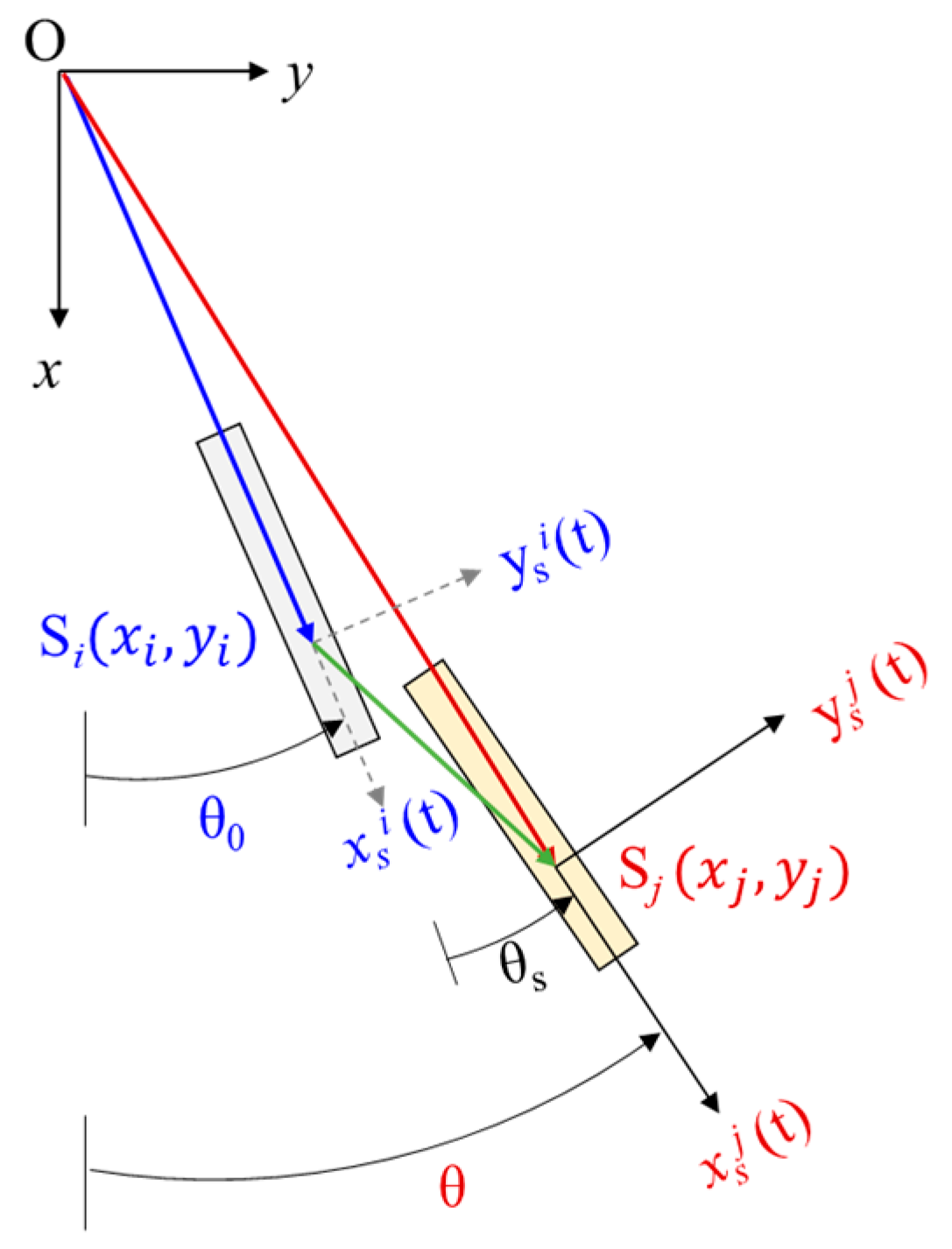
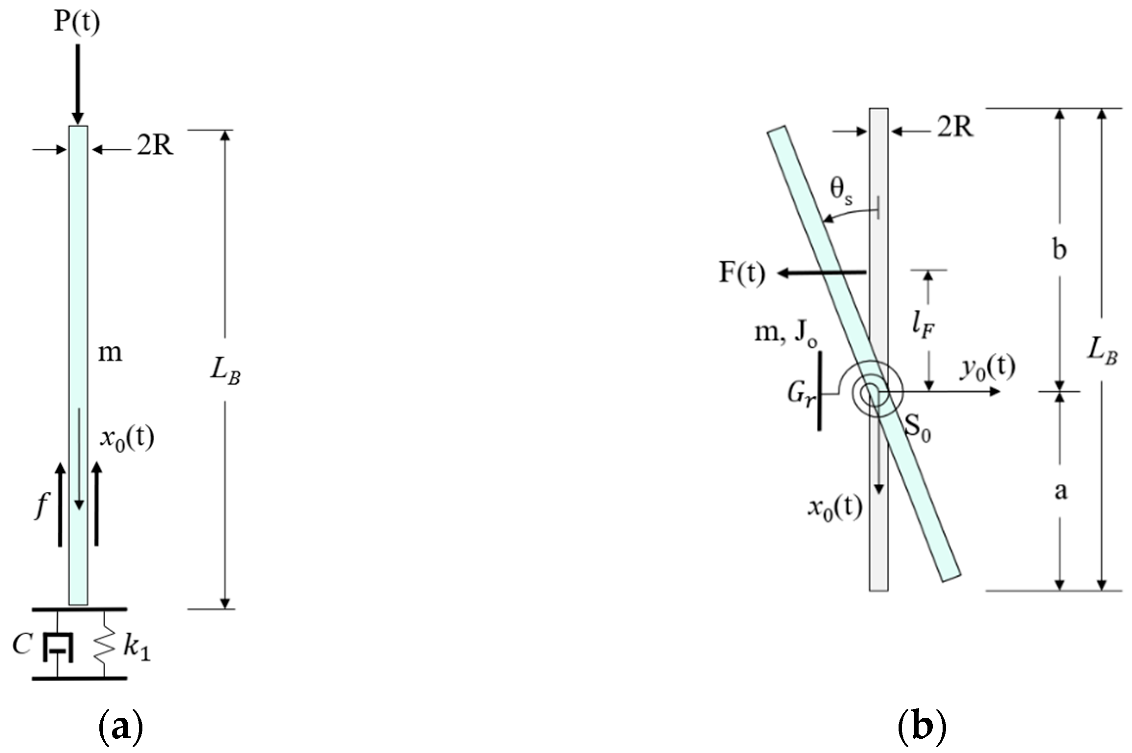
2.1. Model Description

As illustrated in Figure 1, a wireline mole-like underground burrowing robot can realize locomotion in a granular medium. In this work, the drilling motion is simplified and decoupled into two in-plane translations and one in-plane rotation, representing the direction of moving advance. A 3D model may be developed on the basis of this work in the future to consider the out-of-plane deviation of this plane by the coordinate transformation.
The autonomous burrowing robot is assumed to be a rigid cylindrical rod, because it is relatively stiffer than the lunar regolith. This type of assumption is widely accepted in the geotechnical field [33,44,45]. The fundamental problem is actually simplified as the dynamic interaction of the rigid rod with the elastic response of lunar regolith. Furthermore, the resistive interactions in the axial, lateral, and rotational direction are modeled as the axial, lateral spring, and torsional springs [46]. The underground locomotion excavates and transports the regolith and rocks onto the ground. In this proposed model, this excavating process is not considered and only the drilling process is described.
The cylindrical rod is described by its body length, L B , cross-sectional diameter, 2R, and a uniformly distributed mass, m. To describe the rotation, the rotational center, S i (in the i-th state of the numerical step), is assigned at a position as the distance of a from the bottom, and b from the top, as shown in Figure 2. In steering mode, the deflection of the drilling rod is driven by the lateral thrust, F t , which acts on the position with a distance of l F from the center of rotation. The axial thrust force drives the forward motion along the axial orientation of the drilling rod, denoted as P t . The weight on the bit (WOB) is the reaction force of the resisted drilling rod moving forward, which is mathematically simplified as the axial stiffness in the contact model. Similarly, the lateral reaction and anti-rotational torques are represented by two lateral and torsional contact springs. The friction force around the cylindrical rod is symbolled as f . Therefore, the resistive forces and torques can be estimated by the contact stiffness of the regolith.

2.2. Dynamic Equations

Two coordinate systems are introduced here: an Eulerian one fixed in the global space and a Lagrangian one attached to the rigid beam, as shown in Figure 3. The Eulerian global system is introduced by a Cartesian coordinate to record the location ( x , y ) of the rotating center. A spatial variable of θ is defined to record the deflection of the 2D body corresponding to the current location ( x , y ). A full kinematic history of locomotion ( x , y , θ ) is recorded in the global coordinate system.
The local coordinate system is attached to the rigid beam with a Cartesian coordinate. The origin of local Cartesian coordinate is set in the rotating center. The locomotive displacement is discretized into a series of sequential increments described in local coordination ( x s i , y s i ) fixed on the body. Here, i represents the i -th state. The axis of x s is aligned with the body axis of the rod.
The kinematics of locomotion are described by the Lagrangian type with the local coordinates of the x s -axis and y s -axis for the translational directions. The rotational center, Si ( x s i , y s i ), and Sj ( x s j , y s j ) are defined as the origin of the local Cartesian coordinate for two states: initial state and end state during one discretized time increment. The spatial variable of in-plane rotation, θ s , around the rotating center is recorded during the increment from the i -th to the j -th state in the local coordinate. The angular rotation of the rod in global Cartesian coordinate θ is updated based on the in-plane rotation, θ s , after a stepwise motion. In this way, the in-plane penetration and deflection of a rigid robot are well decomposed and described by three components, respectively. The total time period is divided evenly with an equal time step.
Several assumptions are made in the numerical scheme: (i) each time step leads to the small amplitude of 3-DOFs ( x s , y s , θ s ); (ii) the axial thrust, P, is applied coaxially with the rod, and lateral thrust, F, is applied transversely to the moving body; (iii) the resistive stiffnesses of the lunar regolith are idealized as three components: two compressive stiffnesses of k 1 in the x -direction and k 2 in the y -direction, and one torsional stiffness, G r . These three terms of stiffnesses are defined as the characteristics of different layered formations corresponding to a vertical depth of x .
The kinematics of the motion are described in the global coordinate; the coordinates ( x , y ) and spatial variable ( θ ) are calculated based on the initial and end states at each individual step. The coordinates ( x , y ) and spatial variable ( θ ) of the current configuration are given as:
q = q 0 + T e q s
where the matrix of the current displacement in the global coordinate is q , the initial position in the global coordinate is q 0 , the matrix of the local displacement is q s , and the coordinate transformation matrix of displacement is T e :
q = x y θ ,   q 0 = x 0 y 0 θ 0 ,   q s = x s y s θ s
T e = cos θ 0 sin θ 0 0 sin θ 0 cos θ 0 0 0 0 1
where x , y , and θ represent the position and rotation of the current configuration of a finite length rod in the global coordinate; x 0 , y 0 , and θ 0 represent the ones of the initial (or previous) configuration in the global coordinate; and x s , y s , and θ s represent the ones of the current configuration in the local coordinate.
The translational and angular velocity components are then calculated by differentiating the coordinate x , y , and θ directly, as follows:
q ˙ = q ˙ 0 + T ˙ e q s + T e q ˙ s
where the matrix of the current velocity in the global coordinate is q ˙ , the initial velocity in the global coordinate is q ˙ 0 , the matrix of the local velocity is q ˙ s , and the coordinate transformation matrix of velocity is T ˙ e :
q ˙ = x ˙ y ˙ θ ˙ ,   q ˙ 0 = x ˙ 0 y ˙ 0 θ ˙ 0 ,   q ˙ s = x ˙ s y ˙ s θ ˙ s   ,   T ˙ e = T e t
Based on Lagrangian mechanics, the dynamic description of a rigid rod with 3-DOF can be formulated by the following steps:
(i) The kinetic energy of the system, including the translation and rotation, is expressed as:
T = 1 2 m x ˙ 2 + y ˙ 2 + 1 2 J 0 θ ˙ 2
where the rotational inertia, J 0 , is calculated as J 0 = m a 3 + b 3 / 3 L B .
(ii) The potential energy of the system is induced by the deformation from the lunar regolith, which is given as:
U = 1 2 k 1 x s 2 + 1 2 k 2 y s 2 + 1 2 G r θ s 2
(iii) The Lagrangian function is defined by:
L = T U
(iv) Based on classical mechanics, the Lagrange equations are given as:
d d t L q ˙ s k L q s k = Q k   ,   k = 1 , 2 , 3
where generalized coordinates q s 1 = x s ,   q s 2 = y s , q s 3 = θ s and generalized forces Q 1 = P f ,   Q 2 = F ,   Q 3 = F l F . The friction force, f = μ ρ g x s π R L B , is defined as a function of planet gravity and the diving depth according to classical soil mechanics. For simplification, μ = 0.1 is assumed to be the coefficient of robot–soil friction in this work.
(v) Finally, the Lagrangian equations for this problem are obtained as the following ordinary differential equations (ODEs):
M ( q ¨ s + T e T q ¨ 0 ) + C q ˙ s + K q s = Q
M = m 0 0 0 m 0 0 0 J o ,   C = C x 2 m θ ˙ 0 0 2 m θ ˙ 0 C y 0 0 0 C θ , K = k 1 m θ ˙ 0 2 m θ ¨ 0 0 m θ ¨ 0 k 2 m θ ˙ 0 2 0 0 0 G r
The numerical damping term of C q ˙ s is added into the left-hand side of Equation (10) as the numerical dissipative terms. Here, the matrix of the numerical damping factors, C , is introduced to avoid the occurrences of infinite values of displacements induced by constant speed at the equilibrium state [47]. Equations (10) and (11) are the governing equations of a self-burrowed steering robot drilling into a general granular medium.

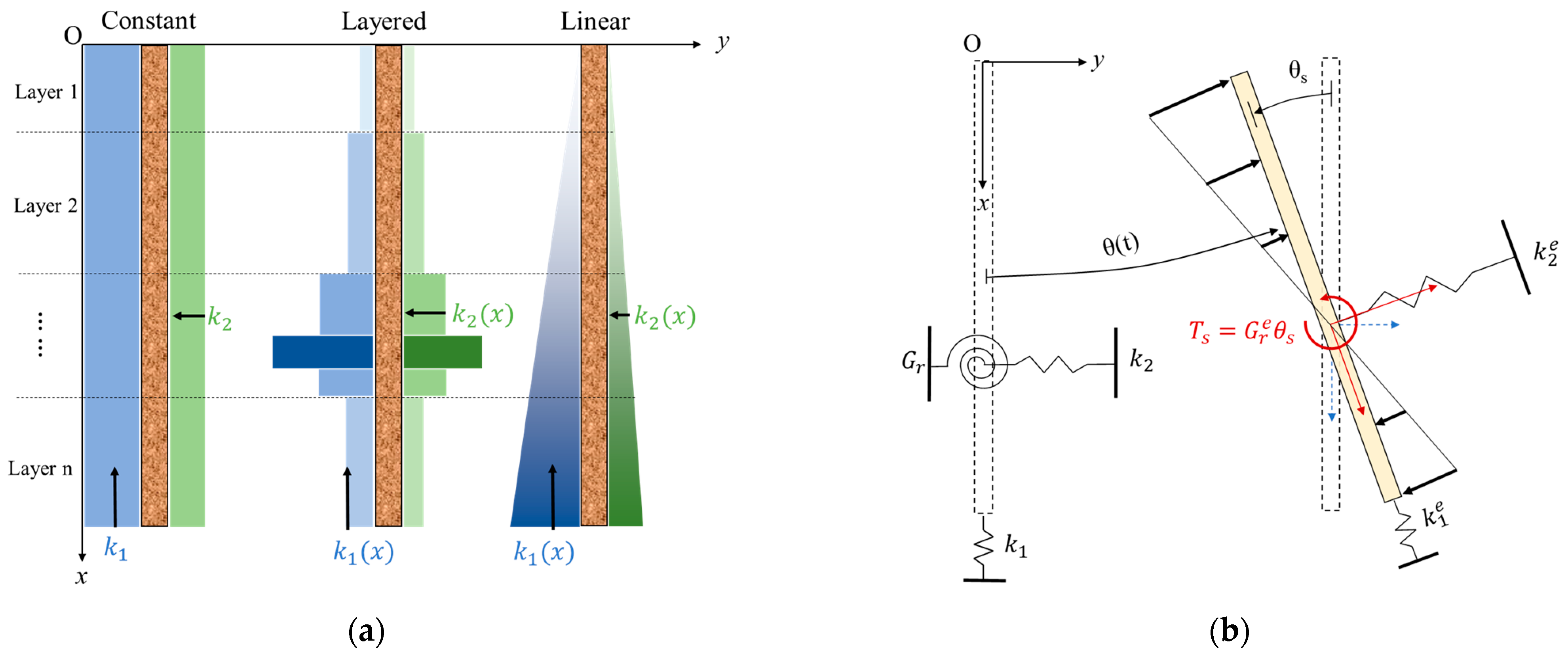
2.3. Soil Interaction Model

The contact interaction between the robotic body and the regolith is described as one set of spring systems. The stiffnesses of the contact springs approximately represent the in situ elastic behaviors of soil or regolith in depth. In reality, these represent various geologic structures, stratigraphic profiles, and complex stress states. In this work, there are three idealized models of resistive-stiffness distribution with the depth-dependence (as shown in Figure 4), but the horizontal variation of the regolith is not considered.
(i) In a uniform subsurface model, the vertical and horizontal stiffnesses of k 1 and k 2 are the constant values through all the depths (noted as “Constant”).
(ii) The formation contains a sequence of stacking layers in the vertical direction, and each layer has an individual constant stiffness (noted as “Layered”):
k i x = k i 1 x 0 ,   d 1 k i 2 x d 1 ,   d 2
where i = 1 , 2 represents the lower index of k 1 ( x ) and k 2 ( x ) , k i 1 , and k i 2 represent the constants of k i at the corresponding depth. The layered formation is segmented by a set of horizontal planes at different depths of x   =   d 1 , d 2 , , etc.
(iii) The formation has a linear distribution of stiffness in depth (noted as “Linear”), respectively. All the vertical and horizontal stiffnesses of k 1 and k 2 are defined at the global coordinate system. The depth-dependent regolith model is assumed as the linear distribution along the depth. The slope of stiffness is noted as δ a v in the vertical direction and δ l v in the lateral direction. k 1 and k 2 are expressed as:
k 1 ( x ) = δ a v x k 2 ( x ) = δ l v x
During the drilling process, the dip angle, θ , and the corresponding depth, x , of the robotic body is changing over time as θ t and x t . Considering the lithological distribution of the regolith in depth, the resistive stiffness acting on the robot is therefore varied with respect to the functions of time, θ t and x t . To describe the resistive stiffnesses at each robotic attitude angle, the effective stiffnesses are introduced as k 1 e and k 2 e along the local coordinated system attached to the robot body. The effective stiffnesses are decomposed as:
k 1 e = k 1 ( x ) cos θ ( t )     k 2 ( x ) sin θ ( t )
k 2 e = k 2 ( x ) cos θ ( t )   +   k 1 ( x ) sin θ ( t )
In the local coordination system, the torsional stiffness, G r e , can be easily calculated based on the variables of a, b, k 1 e , and k 2 e . The effective torsional stiffness, G r e , has a linear relation between the active torsion, T s , and the rotational angle, θ s , because of the small displacement assumption in each iteration.
T s = G r e θ s
where
T s = 0 b k 2 e   L B l 2 d l + 0 a k 2 e   L B l 2 d l
This then leads to:
G r e = b 3 3   L B k 2 ( x ) cos θ ( t ) + k 1 ( x ) sin θ ( t ) + a 3 3   L B k 2 ( x ) cos θ ( t ) + k 1 ( x ) sin θ ( t )
In this work, the research objective is to build a numerical model predicting the dynamic behaviors of a robotic mole burrowing in the lunar subsurface. However, the characterization of the equivalent parameters of lunar regolith is not considered in the scope of this work.

2.4. Numerical Scheme and Nondimensionalized Treatment

To solve this set of ODEs, the integration process is conducted by the Runge–Kutta method [33,35,36]. The iteration is implemented by solving Equations (10) and (11). In between each step, the current coordinate and velocity components in Equations (1)–(5) are updated; these procedures are then repeated for the next time increment, until the final time is reached. In each time step, the ODEs are solved at a constant increment size of time, t , as shown in Figure 5.
A dimensionless term of characteristic time, τ , is introduced to determine the time increment. In order to consider each mode of motion, including axial, lateral, or rotational movements, the time, t , is scaled by the corresponding angular resonance period individually as:
τ 1 = t / t 1 ,   τ 2 = t / t 2 ,   and   τ r = t / t r
where the angular resonance periods are defined as the following expressions:
t 1 = 2 π m / k 1
t 2 = 2 π m / k 2
t r = J o / G r
In the case of the rod burrowing with directional controls, the motion is decomposed with three components simultaneously. Therefore, the dimensionless time for the integration is chosen by the axial translation one, τ 1 , as a unified simplification. The size of the time increment, t , is chosen as one-tenth of the dimensionless time, t = 1 10 τ , and a detailed discussion is presented in Section 3.2.
For the other variables, the dimensionless displacements are defined as x ¯ = x / L B and y ¯ = y / L B by scaling with the length of the cylindrical rod. The dimensionless moving velocities, x ˙ ¯ = x ˙ / v 1 and y ˙ ¯ = y ˙ / v 2 , are defined by the velocity divided by the characteristic velocities v 1 = L B / t 1 and v 2 = L B / t 2 . The dimensionless thrust force is defined as P ¯ = P / k 1 L B , and dimensionless torque is defined as M ¯ = F l F / G r .

2.5. Implementation of PD Tracking Control Strategies

Robotic actuator or prototype designs usually require a simple mathematical model to calculate the power consumption required to supply them. The trajectory induces the variation of the amount of power input during the locomotion, which results in pursuing an optimal control strategy. In this proposed model, the output variables of actuations in the burrowing robot are the thrust and lateral forces. A PD control method [48] coupled with ODEs (PD-ODEs) is proposed to estimate the dynamic outputs of thrust and lateral forces required to operate actuators or motors in burrowing robot travelling along a given path.
With PD control strategies, the main purpose is to build the connection between the designed variables (such as displacements and velocities) and the calculated values in each time step. The calculation is conducted in the local coordinate system fixed in the robotic body. To obtain the values of thrust and lateral force by following the specified trajectory, the differences between the desired and calculated displacements and velocities are added as the right side in the Lagrange equations of Equation (10).
Thus, the generalized forces are formulated in a new way. The dynamic model of directional drilling with the PD controller is given as follows:
M ( q ¨ s + T e T q ¨ 0 ) + C q ˙ s + K q s = Q P D
where Q P D is defined as:
Q P D = K P T e T q d q s + K D T ˙ e T q ˙ d q ˙ s
where q d is the designed trace or predefined locomotive trajectory and q ˙ d is the reference velocity calculated based on the specified trajectory. The parameters of   K P = k p 1 k p 2 k p 3 T and K D = k D 1 k D 2 k D 3 T are the gain coefficients of proportional and derivative events, respectively. The superscripts in the gain coefficients of PD, 1, 2, or 3, represent the components in the axial, lateral, or rotational direction of local coordinates, individually. In this calculation process, the PD control model is solved with ODEs in each iteration step, as shown in Figure 6.

3. Studies of Numerical Procedures

In this section, the parameters of numerical damping in ODEs and iterative time step size are discussed in detail. The parameters of the simulation are given in Table 1.

3.1. Numerical Damping

The interaction between locomotive rod and regolith is important and complicated due to the uncertainty of soil compressibility, granular shape, characteristics of locomotion, etc. During the penetration process, the regolith may be compressed or sheared by the locomotive rod. The granular particles in the zone of rod–regolith interaction are forced to slip or rotate, which produces dissipative effects that slow down the locomotion. In general, the dashpot model is introduced to describe the frictional effects of soils on the rod [49,50]. Theoretically, the dashpot model represents energy loss due to friction [51]. The numerical damping factor in this work is introduced based on the practical circumstance. This factor is numerically correlated to the system and the properties of the soil medium, but it is not a physical variable. It can be determined by additional calibration experiments in order to compare the physical experiments.
For illustration, two simple cases with a 1-DOF movement are studied: the motion of penetration at a constant thrust and deflection at a constant moment of rotation, as shown in Figure 7. In the first case, only the x terms of Equation (10) are considered, and the spatial variable, θ , is not considered. The magnitude of the driving force, P ¯ , is studied here. In the second case, all terms in Equation (10) are considered, but only the driving torque, M ¯ , is applied, and the gravitational effect is disregarded.
To discuss the effects of damping factor on the results, factor C x , with different values of 0.1, 1, and 10, and factor C θ , with different values of 1, 10, and 100, are compared, as follows. As shown in Figure 8, the displacement and velocity reach the lower (blue) curve due to the higher value of C x or C θ . This shows that the damping factor contributes to the frictional energy loss and suppresses the increases of displacement and velocity. In this work, the value of C x is set as 10, and C θ is set as 100.

3.2. Time Step Size

To discuss the effects of increment size of time, Δt, the values of Δt = τ, τ/10 and τ/100 are compared with C θ = 10. As shown in Figure 9, there are tiny differences between the results, with Δt = τ, τ/10 and τ/100 (curves with black, red, and blue colors are actually overlapped). The results indicate that increment size of time, Δt (within the studied range), only affects the sampling rate, but not the results.

4. Numerical Experiments

In this section, four sets of numerical experiments are discussed in detail, including the numerical verifications of simple loading cases, trajectory tracking control, steerability, and directional drilling in different geological formations.

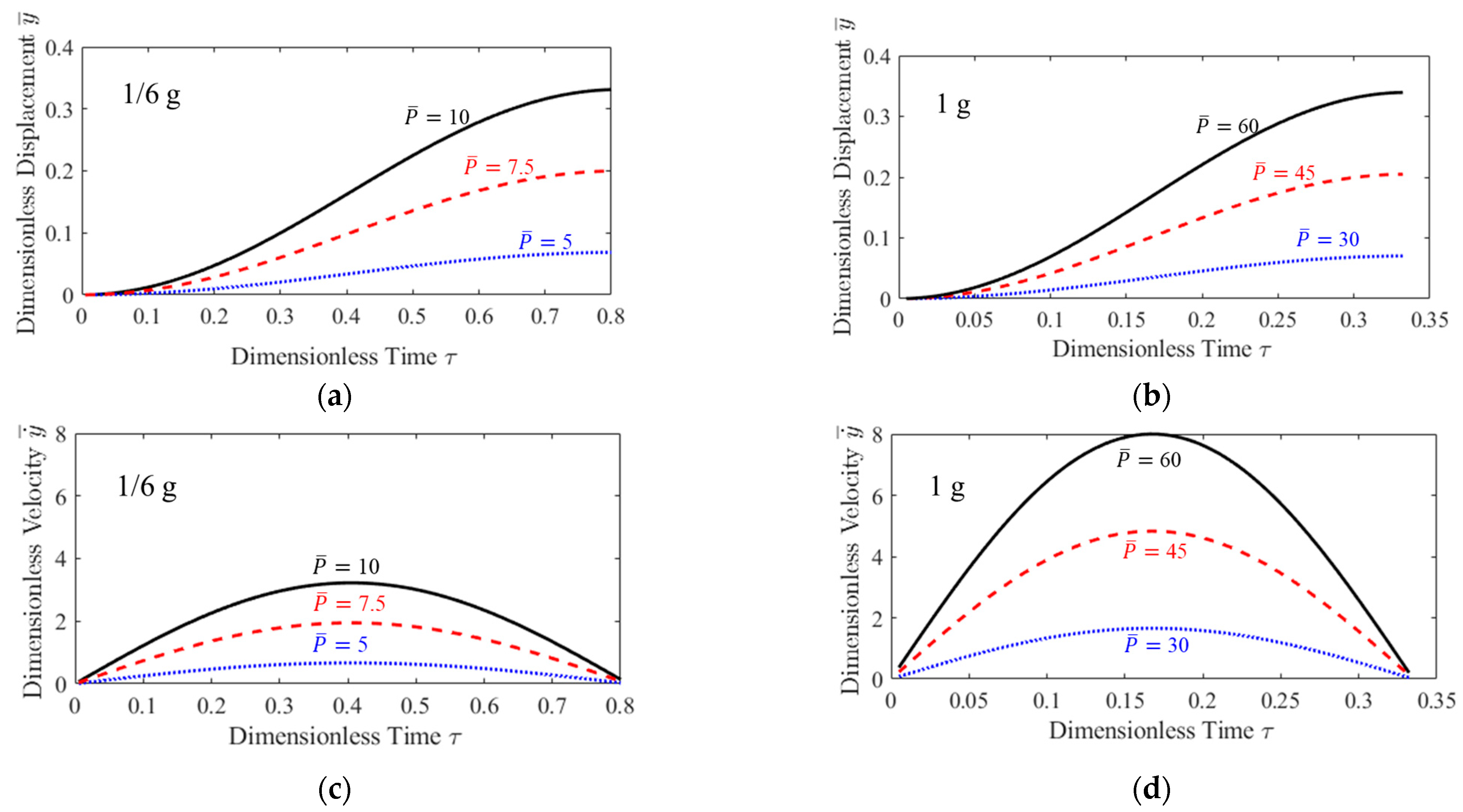
4.1. 1-DOF Movement in a Uniform Formation: Earth vs. Moon

Firstly, two simple scenarios, with one single DOF movement, are further studied, as shown in Figure 7. One is the penetration process driven by the axial thrust, and the other is the deflection of the rod embedded in the regolith induced by the lateral moment.

4.1.1. Case I of Penetration

In this case, three values of P ¯ (5, 7.5, and 10) are compared in Figure 10a,c under 1/6 Earth gravity of the Moon (1/6 g). In contrast, the values of P ¯ (30, 45, and 60) are compared in Figure 10b,d under an Earth gravity of 1 g. Both nondimensionalized displacement and velocity are plotted in the solid line and dotted line, respectively. The maximum dimensionless displacement is predicted under the constant driving force. The higher driving force leads to a deeper and faster penetration. This agrees well with the phenomena of punching the rod into soils in geotechnical engineering [20]. The main parameters used in the simulation are listed in Table 1.
The results in Figure 10a,c represent the case of 1/6 g on the Moon. To consider the gravity effect, the case of 1 g on the Earth is illustrated in Figure 10b,d. The maximum displacement under 1 g is reduced to roughly 1/6 compared to ones under 1/6 g at six times P ¯ . The amplitude of velocity is faster than the ones under 1/6 g, because of the higher kinetic energy of six times the level of P ¯ . It should be mentioned that the case of P ¯ = 5 cannot penetrate the soil to the same depth due to the high overburden pressure on the Earth. Therefore, the P ¯   required on the Earth to penetrate the same depth is roughly six times that on the Moon.

4.1.2. Case II of Deflection

In this case, three values of M ¯ (0.1, 0.5, and 1) are compared in Figure 11. The higher M ¯ = F l F / G r leads to the larger deviation of the steerable robot. The angular rotation reaches a limited value, and the angular velocity reduces gradually to zero at a constant torque due to the resistance of the soil.

4.1.3. Case III of in-Plane Directional Movement

Locomotion with directional controls is decomposed with three components ( x ,   y ,   θ ) simultaneously. The value of F/P is defined as the ratio of lateral to axial thrust. To discuss the effect of F/P, three values of F/P of 0.01, 0.02, and 0.05 are compared.
To investigate the contribution of P or F individually, one component of P or F is set as a constant, and another is set as a variable. Therefore, there are two situations: the directional motion with either the same value of lateral thrust or axial thrust, which is noted as “Constant P” or “Constant F”, respectively. It should be noted that the same values of P and F are in the case of F/P = 0.05 under 1/6 g and 1 g. The results of F/P are shown in Figure 12. The high value of F/P means there is a high potential to deflect and a low potential to penetrate, and vice versa. This nondimensionalized value is a crucial parameter to steer the robot and build up the curvature of the burrowing trajectory. For consideration of the gravity, the same value of F/P can drive the robot easier under lunar gravity (1/6 g) than the one under the Earth’s gravity (1 g). To summarize, the amplitude of the movement can be magnified by approximately six times from the Earth to the Moon under the same power consumption.

4.2. Trajectory Tracking via PD Control

To track a specified trace with PD control strategies, the difference between the given and predicted values of the displacements and velocities are the important quantities in PD-ODEs. Therefore, the performances of tracking are compared in terms of both the displacements and the velocities between the predicted and specified trajectory. In this case, k 1 and k 2 are set as a constant of the depth-independence. The main parameters used in the simulation are listed in Table 2.
The dogleg severity (DLS) is a measure of the change in direction of a well bore over a defined length, which is widely used for the oil and gas application to describe how the wellbore trajectory changes rapidly [52]. DLS is a terminology here to compare the curvature of trajectories or the robotic capability of steering. The DLS of trace is characterized by the curvature radius, Rs, and its rotation angle, θ R , as shown in Figure 13a.
One trajectory is designed as shown in Figure 13b and partitioned into three segments of 1, 2, and 3. The segments represent three stages of drilling: the vertical penetrating locomotion (blue shading), steering (yellow shading), and then locomotion along its tangential direction (white shading), respectively. In this case, the curvature radius (Rs) and its rotation angle ( θ R )are set as constants, where θ R is the same value of 3° and the curvature radius, Rs, is 100 m.
Here, the simulations of directional motion are conducted with the set of parameters   k 1 = 10 N/m, k 2 = 5 N/m, Rs = 100 m, and θ R = 3°. As the results show in Figure 14, the prediction follows well with the specified trajectory in both displacements and velocities. The fluctuation in the predicted velocities is due to the continuous adjustment during the steering motion and stepping into segment 3. The coupled PD method has the capability of tracking the pre-defined trajectory. The robot drills and reams a tubular-shaped borehole in the subsurface block during the directional drilling. The borehole diameter, R c , varies along the movement direction when the robot builds up a 3D curved tunnel, as shown in Figure 15a. The value of Rc/R is introduced as the ratio of actual borehole radius vs. the robotic body’s radius. Here, R c is defined as the projected radius of robotic cylinder body length perpendicular to the normal direction of a specified path. A simulated result is shown in Figure 15b. The plotted circles of Rc/R through this work are scaled by a magnified factor of 2 for a clear visualization of wellbore size. The color bar is normalized from the radius, R, to the diameter, 2R, of the robot. As illustrated, R c increases from segment 1 to segment 2. Near the end of segment 2, the R c decreases to R again, because the attitude angle of the robot is not deviating to ream the hole.

4.3. Parametric Studies on Steerability

4.3.1. Effect of the Curvature of Planned Trajectory

To investigate the performance of steering motion at the given trace, three DLS cases with a different curvatures radius, Rs, but the same rotation angle, θ R , of 3° are considered. The cases of Rs = 30 m, 100 m, and 300 m are simulated and compared, as shown in Figure 16. DLS is determined by the curvature, Rs, and a smaller Rs leads to a higher DLS or wellbore curvature. In this case, the drilling domain of interest is assumed to be the constant one with k 1 = 10 N/m and k 2 = 5 N/m.
The simulations are conducted under different specified paths with DLSs of Rs = 30 m, 100 m, and 300 m. As shown in Figure 17, the computational results indicate that the higher curvature of trajectory produces a larger horizontal movement and higher value of F/P. For the high curvature case, the value of F/P and Rc/R snaps during the locomotion across the segments with different DLSs. For the small curvature case, the shape of the wellbore becomes slender. This is because, under the relatively smaller DLS, the gradient of variation of the trace is actually smoother. Thus, the robot tends to adjust more easilly under the path with a smaller DLS. Actually, the variation of Rc/R along the trajectory relates to the steerability, manipulation, and energy consumption of a robot.

4.3.2. Effect of the Rotation Center in the Robotic Body

As shown in Figure 2, the ratio of a/b is defined as the relative rotation center of a steering robot. In this case, the arm length of lateral force is set the same as b. This ratio represents the coupled relationship between the rotation and the arm length of lateral force.
In this case, the given trajectory is defined as shown in Figure 13b. As shown in Figure 18, the value of a/b = 1 has the optimal bore hole diameter, but the values of a/b = 0.25 and 4 tend to have the higher Rc/R in the steering segment. The maximum Rc/R is produced at a/b = 4. Limited by its short arm length of lateral force, this makes it hard to offer a sufficient capability to steer. The results indicate that to meet the requirements for a fine tuning of attitude angle, the structural parameter a/b of the robot should be carefully considered in the design, especially with the limited steering capacity of actuators.

4.3.3. Effect of the Moving Velocity Control

In this section, the velocity control along the path is discussed. The velocity of steering the robot along the directional path is assumed to be a constant. These pre-set velocities are actually the resultant speeds, denoted as V s . Its components in both the axial and lateral directions are accordingly calculated based on the location of the robot along the pre-planned trajectory, as shown in Figure 13b.
The results of simulation are compared in Figure 19 for different targeted velocities ( V s ) of 1 mm/s, 5 mm/s, 10 mm/s, and 20 mm/s. The maximum Rc/R is decreased with the higher value of velocity. In the transition region between segments 1 and 2, the value of Rc/R is lower under the velocity of 1 mm/s. In contrast, the value of Rc/R is smaller with the faster locomotive velocity during the transition region between segments 2 and 3. The higher velocity might not give a sufficient time for the robot to adjust its orientation properly at the start, that is, the transition region between segments 1 and 2. The difference between the simulation and designed values of displacements and velocities in PD-ODEs is relatively greater under a higher velocity. Thus, an intense response in iterative steps might appear in these situations ( V s = 5 mm/s, 10 mm/s, and 20 mm/s). Accordingly, the value of F/P is increased with the rise in velocity. In the case of constant cruising speed, a high velocity could lead to a strong counteracting resistance, and therefore consume additional power to manipulate.

4.4. Directional Drilling in Different Geological Formations

4.4.1. A Layered Formation Model with a Set of Constant Stiffnesses

The interaction between the rod and regolith is described by three parameters: the compression stiffness, k 1 , in the x- direction and k 2 in the y-direction, and the torsional stiffness, G r . In this case, the stiffness coefficients are assumed to be constant layer by layer. To describe the effective stiffness in the robot at its local coordinated system, k 1 , k 2 , and G r are transferred to k 1 e , k 2 e , and G r e in a local coordinated system during each simulated iteration step, as described in Section 2.3. Here, the ratio of k 2 / k 1 is set as a constant value of 0.5 in all cases. For the comparison of cases, the pre-defined trajectory is the same one as for curvature radius Rs = 100 m and rotational angle   θ R = 3°, as shown in Figure 13b. The cruising speed, V s , is set at the same value of 2 mm/s.
The regolith zone is defined as a three-layered structure; the vertical stiffness of segment 1, 2, and 3 is set as 1 N/m, 100 N/m, and 1 N/m, respectively, noted as k 1 = 1:100:1. It is numerically expressed in the following way:
k 1 x = 1 x 0 ,   2 100 x 2 ,   7.3    1 x 7.3 ,   10
The lateral stiffness is fixed and determined as k 2 / k 1   = 0.5 in all cases. This situation corresponds to the reality of drilling into a hard formation layer from a soft layer. The simulated results are also compared with three uniform formation models under constant stiffness values of k 1 = 1, 50, and 100 N/m, respectively, and a layered formation with k 1 = 1:100:1. The results are shown in Figure 20. The locomotion in “harder” regolith could lead to a more elongated borehole shape compared with different k 1 . When there is a layered distribution of stiffness in depth, the segment with a “hard” formation actually helps the robot to maintain a good steering stability and adjustment of its attitude angle.

4.4.2. A Formation Model with a Linear Distribution of Stiffness

Considering the actual condition of the layered structure of regolith, stiffness k 1 in the x-direction and k 2 in the y-direction, and the torsional stiffness, G r , may vary with the depth direction due to overburden [53,54]. Furthermore, a depth-dependent stiffness can provide the high-fidelity prediction to simulate a practical robot–soil interaction for deep drilling on the Moon.
In this comparison, the given tracking path is determined with Rs = 100 m and θ R = 3°, as shown in Figure 13b. The cruising speed, V s , is a constant of 2 mm/s. As shown in Figure 21, three slopes of linear formations are considered, δ a v = 1, 1.5, and 2 N/m2, with the lateral stiffness ratios of k 2 k 1 = 0.5 ( δ a v / δ l v = 0.5). With the same set of parameters, steering in media of the higher stiffness, it can achieve the higher angular deflection. This indicates that, to some extent, steering in regolith with a higher (both vertical and lateral) stiffness makes it easier to adjust the attitude angle of the burrowing robot with a good stability.
In the case of a linear depth-depended stiffness distribution, the stiffness ratio of k 2 / k 1 is defined by the value of δ l v / δ a v . The overburden and confining pressures in the layered soil are represented in the value of k 2 / k 1 . To investigate the effect of a stiffness ratio of k 2 / k 1 on the steering, the linear slope of vertical stiffness is set at a constant of δ a v = 1 N/m2, and the ratios of k 2 / k 1 (which equals δ l v / δ a v ) is set as 0.5, 1, and 2, respectively. As the results show in Figure 22, the higher stiffness ratios of k 2 / k 1 leads to a slenderer wellbore geometry.
Overall, the results show that the different conditions of DLS of the designed trace, locomotive velocity, and possible stiffness of layered soils can influence the tracking performance of a self-burrowing robot. Currently, PD parameters are given as a certain set of values, so it is not necessary to strictly follow the desired path. In the near future, the control algorithm will be investigated in more details.

5. Conclusions

In this work, a predictive model of a self-locomotive burrowing device is proposed. A set of 3-DOF governing equations is derived to describe the kinematic states of a mole-like drilling robot. The trajectory and kinematics of locomotion is predicted numerically with the implementation of the Runge–Kutta method. The coupled equations with the proportional-derivate control method are developed to estimate the F/P and Rc/R along the prescribed trajectory. Parametric studies with planned trajectories, planet gravity, formations, and structural parameters are investigated for understanding the steerability and capacity of actuation during the drilling process.
The proposed reduced-order model serves as a simplified tool to simulate the operating and controlling scenarios of an autonomous burrowing robot within the lunar subsurface. It also provides an estimation of the operating difference between drilling experiments in a lunar environment and on Earth. It may be further expanded to consider full 3D trajectory planning and navigation algorithms coupled with the in-time subsurface imaging techniques of LPR and data-driven digital-twin development.
All in all, this model provides an initial attempt to plan the space missions of a drilling robot to obtain regolith samples through deep drilling within an extraterrestrial planet such as the Moon or Mars.

Author Contributions

Conceptualization, H.Z. and Z.Y.; methodology, Z.Y., R.M. and H.Z.; software, Z.Y. and R.M.; validation, Z.Y.; investigation, Z.Y.; writing—original draft preparation, Z.Y.; writing—review and editing, H.Z.; supervision, H.Z.; project administration, H.Z. and K.W.; funding acquisition, H.Z. and K.W. All authors have read and agreed to the published version of the manuscript.

Funding

H.Z. acknowledges the support from the China Manned Space Engineering Program and the Innovative Research Fund of the Chinese Academy of Sciences, through Grant No. JCPYJJ-22002. R.M. acknowledges support from the Innovative Research Fund of the Key Laboratory of Space Utilization, Chinese Academy of Sciences, under Grant No. CSU-JJKT-2020-5.

Data Availability Statement

The datasets generated and supporting the finds of this article are available from the corresponding author upon request.

Conflicts of Interest

The authors declare no conflict of interest.

References

  1. Aguilar, J.; Zhang, T.; Qian, F.; Kingsbury, M.; McInroe, B.; Mazouchova, N.; Li, C.; Maladen, R.; Gong, C.; Travers, M.; et al. A review on locomotion robophysics: The study of movement at the intersection of robotics, soft matter and dynamical systems. Rep. Prog. Phys. 2016, 79, 110001. [Google Scholar] [CrossRef] [Green Version]
  2. TZhang, T.; Wang, B.; Wei, H.; Zhang, Y.; Chao, C.; Xu, K.; Ding, X.; Hou, X.; Zhao, Z. Review on planetary regolith-sampling technology. Prog. Aerosp. Sci. 2021, 127, 100760. [Google Scholar] [CrossRef]
  3. Gorevan, S.P.; Myrick, T.M.; Batting, C.; Mukherjee, S.; Bartlett, P.; Wilson, J. Strategies for future Mars exploration: An infrastructure for the near and longer-term future exploration of the subsurface of Mars. In Proceedings of the 6th International Conference on Mars, Pasadena, CA, USA, 20–25 July 2003; pp. 20–25. Available online: https://ui.adsabs.harvard.edu/abs/2003mars.conf.3196G/abstract (accessed on 1 February 2023).
  4. Heiken, G.H.; Vaniman, D.T.; French, B.M. Lunar Sourcebook, a User’s Guide to the Moon; Cambridge University Press: Cambridge, UK, 1991; ISBN 9789780521332. [Google Scholar]
  5. Larose, E.; Khan, A.; Nakamura, Y.; Campillo, M. Lunar subsurface investigated from correlation of seismic noise. Geophys. Res. Lett. 2005, 32, L16201. [Google Scholar] [CrossRef] [Green Version]
  6. Glass, B.; New, M.; Voytek, M. Future space drilling and sample acquisition: A collaborative industry-government workshop. Icarus 2020, 338, 113378. [Google Scholar] [CrossRef]
  7. Lopez-Arreguin, A.; Montenegro, S. Towards bio-inspired robots for underground and surface exploration in planetary environments: An overview and novel developments inspired in sand-swimmers. Heliyon 2020, 6, e04148. [Google Scholar] [CrossRef]
  8. Barenboim, M.; Degani, A. Steerable Burrowing Robot: Design, Modeling and Experiments. In Proceedings of the IEEE International Conference on Robotics and Automation, Paris, France, 31 May–31 August 2020; pp. 829–835. [Google Scholar] [CrossRef]
  9. Lichtenheldt, R.; Becker, F.; Zimmermann, K. Screw-driven Robot for Locomotion into Sand. In Proceedings of the Ilmenau Scientific Colloquium, Ilmenau, Germany, 11–15 September 2017; pp. 11–15. Available online: https://elib.dlr.de/114033/ (accessed on 1 February 2023).
  10. Olaf, K.; Marco, S.; Fittock, M.; Georgios, T.; Torben, W.; Lars, W.; Matthias, G.; Jörg, K.; Tilman, S.; Christian, K.; et al. Design details of the HP3 mole onboard the InSight mission. Acta Astronaut. 2019, 164, 152–167. [Google Scholar] [CrossRef]
  11. Mizushina, A.; Omori, H.; Kitamoto, H.; Nakamura, T.; Osumi, H.; Kubota, T. A discharging mechanism for a lunar subsurface explorer with the peristaltic crawling mechanism. In Proceedings of the International Conference on Recent Advances in Space Technologies, Istanbul, Turkey, 12–14 June 2013; pp. 955–960. [Google Scholar] [CrossRef]
  12. Zhang, T.N.; Daniel, I.G. The effectiveness of resistive force theory in granular locomotion. Phys. Fluids 2014, 26, 101308. [Google Scholar] [CrossRef] [Green Version]
  13. Treers, L.K.; Cao, C.; Stuart, H.S. Granular Resistive Force Theory Implementation for Three-Dimensional Trajectories. IEEE Robot. Autom. Lett. 2021, 6, 1887–1894. [Google Scholar] [CrossRef]
  14. Gorevan, S.P.; Hong, K.Y.; Myrick, T.M.; Bartlett, P.W.; Singh, S.; Stroescu, S. An Inchworm Deep Drilling System for Kilometer Scale Subsurface Exploration of Mars (IDDS). In Proceedings of the Concepts and Approaches for Mars Exploration, Houston, TX, USA, 18–20 July 2000; p. 1. Available online: http://www.lpi.usra.edu/meetings/robomars/ (accessed on 1 February 2023).
  15. Zhang, W.; Jiang, S.; Tang, D.; Chen, H.; Liang, J. Drilling Load Model of an Inchworm Boring Robot for Lunar Subsurface Exploration. Int. J. Aerosp. Eng. 2017, 2017, 1282791. [Google Scholar] [CrossRef] [Green Version]
  16. Gouache, T.P.; Gao, Y.; Coste, P.; Gourinat, Y. First experimental investigation of dual-reciprocating drilling in planetary regoliths: Proposition of penetration mechanics. Planet. Space Sci. 2011, 59, 1529–1541. [Google Scholar] [CrossRef]
  17. Bar-Cohen, Y.; Zacny, K.; Badescu, M.; Lee, H.J.; Sherrit, S.; Bao, X.Q.; Freeman, D.; Paulsen, G.L.; Beegle, L. Auto-Gopher-2 An Autonomous Wireline Rotary Piezo-Percussive Deep Drilling Mechanism. In Proceedings of the 16th Biennial International Conference on Engineering, Science, Construction, and Operations in Challenging Environments, Cleveland, OH, USA, 9–12 April 2018; pp. 307–316. Available online: http://hdl.handle.net/2014/46258 (accessed on 1 February 2023).
  18. Bar-Cohen, Y.; Badescu, M.; Sherrit, S.; Bao, X.Q.; Lee, H.J. Auto-Gopher-2 (AG2)-Autonomous Wireline Rotary Piezo-Percussive for Deep Drilling. In Proceedings of the Lunar ISRU 2019-Developing a New Space Economy Through Lunar Resources and Their Utilization, Columbia, MD, USA, 15–17 July 2019; Volume 2152, p. 5104. Available online: https://ui.adsabs.harvard.edu/abs/2019LPICo2152.5104B/abstract (accessed on 1 February 2023).
  19. Williams, B.J.; Anand, S.V.; Rajagopalan, J.; Saif, M.T.A. A self-propelled biohybrid swimmer at low Reynolds number. Nat. Commun. 2014, 5, 3081. [Google Scholar] [CrossRef] [Green Version]
  20. Texier, B.D.; Ibarra, A.; Melo, F. Helical Locomotion in a Granular Medium. Phys. Rev. Lett. 2017, 119, 068003. [Google Scholar] [CrossRef] [Green Version]
  21. Maladen, R.D.; Ding, Y.; Umbanhowar, P.B.; Kamor, A.; Goldman, D.I. Mechanical models of sandfish locomotion reveal principles of high performance subsurface sand-swimming. J. R. Soc. Interface 2011, 8, 1332–1345. [Google Scholar] [CrossRef] [Green Version]
  22. Kang, W.; Feng, Y.; Liu, C.; Blumenfeld, R. Archimedes’ law explains penetration of solids into granular media. Nat. Commun. 2018, 9, 1101. [Google Scholar] [CrossRef] [Green Version]
  23. Feng, Y.; Blumenfeld, R.; Liu, C. Support of modified Archimedes’law theory in granular media. Soft Matter 2019, 15, 3008–3017. [Google Scholar] [CrossRef]
  24. Cundall, P.A.; Strack, O.D.L. A discrete numerical model for granular assemblies. Géotechnique 1979, 29, 47–65. [Google Scholar] [CrossRef]
  25. Xi, B.; Jiang, M.; Cui, L. 3D DEM analysis of soil excavation test on lunar regolith simulant. Granul. Matter 2021, 23, 1. [Google Scholar] [CrossRef]
  26. Kawamoto, R.; Andò, E.; Viggiani, G.; Andrade, J.E. All you need is shape: Predicting shear banding in sand with LS-DEM. J. Mech. Phys. Solids 2018, 111, 375–392. [Google Scholar] [CrossRef] [Green Version]
  27. Khademian, Z.; Kim, E.; Nakagawa, M. Simulation of Lunar Soil with Irregularly Shaped, Crushable Grains: Effects of Grain Shapes on the Mechanical Behaviors. J. Geophys. Res. Planets 2019, 124, 1157–1176. [Google Scholar] [CrossRef] [Green Version]
  28. Askari, H.; Kamrin, K. Intrusion rheology in grains and other flowable materials. Nat. Mater. 2016, 15, 1274–1279. [Google Scholar] [CrossRef]
  29. Kamrin, K. Nonlinear elasto-plastic model for dense granular flow. Int. J. Plast. 2010, 26, 167–188. [Google Scholar] [CrossRef] [Green Version]
  30. Kim, S.; Kamrin, K. Power-Law Scaling in Granular Rheology across Flow Geometries. Phys. Rev. Lett. 2020, 125, 088002. [Google Scholar] [CrossRef]
  31. Gerolymos, N.; Gazetas, G. Winkler model for lateral response of rigid caisson foundations in linear soil. Soil Dyn. Earthq. Eng. 2006, 26, 347–361. [Google Scholar] [CrossRef]
  32. De Rosa, M.; Maurizi, M. The influence of concentrated masses and pasternak soil on the free vibrations of euler beams—Exact solution. Journal of Sound and Vibration. J. Sound Vib. 1998, 212, 573–581. [Google Scholar] [CrossRef]
  33. Richard, T.; Detournay, E.; Fear, M.; Miller, B.; Clayton, R.; Matthews, O. Influence of bit-rock interaction on stick-slip vibrations of PDC bits. In Proceedings of the SPE Annual Technical Conference and Exhibition, San Antonio, TX, USA, 29 September–2 October 2002. [Google Scholar] [CrossRef]
  34. Detournay, E.; Richard, T.; Shepherd, M. Drilling response of drag bits: Theory and experiment. Int. J. Rock Mech. Min. Sci. 2008, 45, 1347–1360. [Google Scholar] [CrossRef]
  35. Liu, Y.; Lin, W.; Chávez, J.P.; De Sa, R. Torsional stick-slip vibrations and multistability in drill-strings. Appl. Math. Model. 2019, 76, 545–557. [Google Scholar] [CrossRef]
  36. Liu, J.; Wang, J.; Guo, X.; Dai, L.; Zhang, C.; Zhu, H. Investigation on axial-lateral-torsion nonlinear coupling vibration model and stick-slip characteristics of drilling string in ultra-HPHT curved wells. Appl. Math. Model. 2022, 107, 182–206. [Google Scholar] [CrossRef]
  37. Wanasinghe, T.R.; Wroblewski, L.; Petersen, B.; Gosine, R.G.; James, L.A.; De Silva, O.; Mann, G.K.I.; Warrian, P.J. Digital twin for the oil and gas industry: Overview, research trends, opportunities, and challenges. IEEE Access 2020, 8, 104175–104197. [Google Scholar] [CrossRef]
  38. Bimastianto, P.; Khambete, S.; AlSaadi, H.; Couzigou, E.; Al-Marzouqi, A.; Chevallier, B.; Qadir, A.; Pausin, W.; Laurent, V. Digital Twin Implementation on Current Development Drilling, Benefits and Way Forward. In Proceedings of the Abu Dhabi International Petroleum Exhibition & Conference, Abu Dhabi, United Arab Emirates, 9–12 November 2020. [Google Scholar] [CrossRef]
  39. Zhang, J.; Zhou, B.; Lin, Y.; Zhu, M.-H.; Song, H.; Dong, Z.; Gao, Y.; Di, K.; Yang, W.; Lin, H.; et al. Lunar regolith and substructure at Chang’E-4 landing site in South Pole–Aitken basin. Nat. Astron. 2021, 5, 25–30. [Google Scholar] [CrossRef]
  40. Molaro, J.; Byrne, S.; Le, J.-L. Thermally induced stresses in boulders on airless body surfaces, and implications for rock breakdown. Icarus 2017, 294, 247–261. [Google Scholar] [CrossRef] [Green Version]
  41. Hagermann, A.; Tanaka, S. Ejecta deposit thickness, heat flow, and a critical ambiguity on the Moon. Geophys. Res. Lett. 2006, 33, 1–5. [Google Scholar] [CrossRef] [Green Version]
  42. Liu, Y.; Yuan, Z.; Li, Y.; Zhao, H.F. A Three-Dimensional Path Planning Method of Autonomous Burrowing Robot for Lunar Subsurface Exploration. In Proceedings of the 2021 6th IEEE International Conference on Advanced Robotics and Mechatronics (ICARM), Chongqing, China, 3–5 July 2021; pp. 710–715. [Google Scholar] [CrossRef]
  43. Li, Y.P.; Huang, L.; Wang, K.; Zhao, H.F. Geometric Reconstruction Method for Predicting Shape of Irregular Rocks under Moon’s Subsurface Using Lunar Penetrating Radar Based on a Deep Learning Algorithm. Electron. Inf. Technol. 2022, 44, 1222–1230. [Google Scholar] [CrossRef]
  44. Yan, Y.; White, D.J.; Randolph, M.F. Penetration resistance and stiffness factors for hemispherical and toroidal penetrometers in uniform clay. Int. J. Geomech. 2011, 11, 263–275. [Google Scholar] [CrossRef]
  45. TVromen, T.; Detournay, E.; Nijmeijer, H.; Van De Wouw, N. Dynamics of Drilling Systems with an Antistall Tool: Effect on Rate of Penetration and Mechanical Specific Energy. SPE J. 2019, 24, 1982–1996. [Google Scholar] [CrossRef]
  46. Yan, Y.; Wiercigroch, M. Dynamics of rotary drilling with non-uniformly distributed blades. Int. J. Mech. Sci. 2019, 160, 270–281. [Google Scholar] [CrossRef]
  47. Meirovitch, L. Methods of Analytical Dynamics; McGraw-Hill: New York, NY, USA, 1970; ISBN 9780486137599. [Google Scholar]
  48. Lin, W.; Chávez, J.P.; Liu, Y.; Yang, Y.; Kuang, Y. Stick-slip suppression and speed tuning for a drill-string system via proportional-derivative control. Appl. Math. Model. 2020, 82, 487–502. [Google Scholar] [CrossRef]
  49. Dai, W.; Yang, J.; Wiercigroch, M. Vibration energy flow transmission in systems with Coulomb friction. Int. J. Mech. Sci. 2022, 214, 106932. [Google Scholar] [CrossRef]
  50. TAmer, T.S.; Bek, M.A.; Nael, M.S.; Sirwah, M.A.; Arab, A. Stability of the Dynamical Motion of a Damped 3DOF Auto-parametric Pendulum System. J. Vib. Eng. Technol. 2022, 10, 1883–1903. [Google Scholar] [CrossRef]
  51. Karatzia, X.; Mylonakis, G. Horizontal Stiffness and Damping of Piles in Inhomogeneous Soil. J. Geotech. Geoenvironmental Eng. 2017, 143, 04016113. [Google Scholar] [CrossRef] [Green Version]
  52. Bradley, H.B. Petroleum Engineering Handbook; Society of Petroleum Engineers: Richardson, TX, USA, 1987; ISBN 97815556301021555630103. [Google Scholar]
  53. Widisinghe, S.; Sivakugan, N. Vertical Stress Isobars for Trenches and Mine Stopes Containing Granular Backfills. Int. J. Géoméch. 2014, 14, 313–318. [Google Scholar] [CrossRef]
  54. Ting, C.H.; Sivakugan, N.; Read, W.; Shukla, S.K. Analytical Expression for Vertical Stress within an Inclined Mine Stope with Non-parallel Walls. Geotech. Geol. Eng. 2014, 32, 577–586. [Google Scholar] [CrossRef]
Figure 1. Conceptual diagram of self-burrowed steering locomotion in the lunar subsurface.
Aerospace 10 00190 g001
Figure 2. Free body diagram of the in-plane locomotion of the burrowing robot with a finite length: (a) free body diagram; (b) equivalent stiffness representation of granular medium.
Aerospace 10 00190 g002
Figure 3. Illustration of the kinematic relation of a moving rod in the granular medium.
Aerospace 10 00190 g003
Figure 4. Illustration of equivalent stiffness model of regolith and its mathematical description: (a) three hypothetical situations of resistive-stiffness distribution in depth, noted as “Constant”, “Layered”, and “Linear”; (b) the effective contact stiffness in the local coordinate system.
Aerospace 10 00190 g004
Figure 5. Schematic diagram of calculation process.
Aerospace 10 00190 g005
Figure 6. Schematic diagram of calculation process with PD control strategies.
Aerospace 10 00190 g006
Figure 7. Diagram of the 1-DOF motion: (a) penetration by the axial thrust; (b) deflection by the lateral thrust (rotational moment).
Aerospace 10 00190 g007
Figure 8. Comparison of numerical damping effects in the 1-DOF case: (a) penetration at a constant thrust; (b) deflection at a constant moment of rotation.
Aerospace 10 00190 g008
Figure 9. The comparison of time stepping size in the 1-DOF rotation case.
Aerospace 10 00190 g009
Figure 10. The motion of penetration at a constant nondimensional thrust: (a) at a constant nondimensional thrust of 5, 7.5, and 10 under 1/6 Earth gravity; (b) at a constant nondimensional thrust of 30, 45, and 60 under Earth gravity; (c,d) are the dimensionless velocities under 1/6 Earth gravity and Earth gravity, respectively.
Aerospace 10 00190 g010
Figure 11. The deflection at a constant moment of rotation at M ¯ = 0.1, 0.5, and 1: (a) angular displacement; (b) angular displacement velocities.
Aerospace 10 00190 g011aAerospace 10 00190 g011b
Figure 12. Directional penetration under a certain ratio between lateral and axial thrust force: (a) the directional motion under lunar gravity (1/6 Earth gravity) by a constant value of axial thrust; (b) the directional motion under lunar gravity by a constant value of lateral thrust; (c,d) the dimensionless displacements under Earth gravity by a constant value of axial thrust and lateral thrust, respectively.
Aerospace 10 00190 g012aAerospace 10 00190 g012b
Figure 13. Diagram of one planned trajectory: (a) the schematic diagram of DLS and a planned trajectory; (b) the planned trajectory of curvature radius Rs = 100 m and rotational angle   θ R = 3°.
Aerospace 10 00190 g013
Figure 14. Comparison of directional motion between simulation and designed regarding displacement and velocity: (a,b) the displacement histories in the vertical and horizontal directions, respectively; (c,d) the velocity histories in the vertical and horizontal directions. In the legend, ‘Sim’ represents the simulated results, and ‘Designed’ represents the specified trajectory or reference velocity.
Aerospace 10 00190 g014
Figure 15. Illustration of borehole development in a directional well: (a) diagram of steering motion based on the reference trajectory; (b) the predicted borehole radius of Rc/R formed by the robotic steering locomotion. Note: the color bar of the legend represents the scale range of Rc/R.
Aerospace 10 00190 g015
Figure 16. Illustration of three designed traces: (ac) the curvature radius Rs = 30 m, 100 m, and 300 m, respectively. The rotation angle θ R is 3° for all.
Aerospace 10 00190 g016
Figure 17. Predictions under different specified paths: (a) the dimensionless displacement and angular rotation of a steering robot; (b,c) the nondimensional variables of F/P and Rc/R varying with the trajectories with different DLSs, accordingly; (d) 3D representations of wellbore shapes corresponding to different planned trajectories. Note: the color bar of the legend represents the scale range of Rc/R.
Aerospace 10 00190 g017
Figure 18. Simulations under different parameters of a specified trace with different a/b ratio of 0.25, 1, and 4: (a,b) the nondimensional variables of F/P and Rc/R, respectively.
Aerospace 10 00190 g018
Figure 19. Simulations of a designed trace with different resultant velocities along the trace: (a) the nondimensional variables of F/P and Rc/R vary with different targeted velocities in the depth direction, accordingly; (b) the borehole shapes are formed under the given velocities. Note: the color bar of the legend represents the scale range of Rc/R.
Aerospace 10 00190 g019
Figure 20. Simulations for different formation models, including three cases of uniform formation: (a) the ratio of Rc/R varies with different models of stiffnesses; (b) the bore hole shapes are formed during drilling through the prescribed paths. Note: the color bar of the legend represents the scale range of Rc/R.
Aerospace 10 00190 g020
Figure 21. Simulations for directional drilling in a formation model with a linear distribution of stiffness.
Aerospace 10 00190 g021
Figure 22. Simulations under different stiffness ratios of k 2 / k 1 = 0.5, 1, and 2 in depth, with the same δ a v of 1 N/m2: (a,b) are the nondimensional variables of F/P and Rc/R, varying with the ratio of k 2 / k 1 .
Aerospace 10 00190 g022
Table 1. Main parameters of simulation.
NamesSymbolsValuesUnits (SI)
Mass of motion bodym1kg
Body length L B 1m
Arm length of lateral thrust, FlF0.8m
Cross-sectional diameter2R0.08m
Ratio of rotational center in lengtha/b0.25/
Vertical stiffness k 1 10N/m
Horizontal stiffness k 2 5N/m
Table 2. Main parameters of simulation with PD control.
NamesSymbolsValuesUnits (SI)
Mass of motion bodym1kg
Body length L B 1m
Arm length of lateral thrust, FlF0.8m
Cross-sectional diameter2R0.08m
Ratio of rotational center in lengtha/b0.25/
Axial proportional-control factor k p 1 1 × 10³kg/s2
Lateral proportional-control factor k p 2 8 × 10³kg/s2
Torsional proportional-control factor k p 3 1 × 10⁴kg·m2/s2
Axial derivative-control factor k D 1 100kg/s
Lateral derivative-control factor k D 2 100kg/s
Torsional derivative-control factor k D 3 1 × 10⁴kg·m2/s
Disclaimer/Publisher’s Note: The statements, opinions and data contained in all publications are solely those of the individual author(s) and contributor(s) and not of MDPI and/or the editor(s). MDPI and/or the editor(s) disclaim responsibility for any injury to people or property resulting from any ideas, methods, instructions or products referred to in the content.

