Remaining Useful Life Prediction for Aero-Engines Using a Time-Enhanced Multi-Head Self-Attention Model

Abstract

Data-driven Remaining Useful Life (RUL) prediction is one of the core technologies of Prognostics and Health Management (PHM). Committed to improving the accuracy of RUL prediction for aero-engines, this paper proposes a model that is entirely based on the attention mechanism. The attention model is divided into the multi-head self-attention and timing feature enhancement attention models. The multi-head self-attention model employs scaled dot-product attention to extract dependencies between time series; the timing feature enhancement attention model is used to accelerate and enhance the feature selection process. This paper utilises Commercial Modular Aero-Propulsion System Simulation (C-MAPSS) turbofan engine simulation data obtained from NASA Ames’ Prognostics Center of Excellence and compares the proposed algorithm to other models. The experiments conducted validate the superiority of our model’s approach.

1. Introduction

The rapid development of industry has led to a considerable increase in transportation and related industries. Due to the fact that the engine is the most essential part of mechanical equipment, its frequent use may result in the deterioration of its performance and, consequently, safety hazards in day-to-day work. As a result, the prediction of the RUL of the engine is one of the most significant technologies in the field of predictive maintenance.

Predictive maintenance is critical in industrial activities. At present, PHM [1] is widely employed in the aviation industry [2,3] as a result of the development of the industrial field. Failure prediction is an essential technology in PHM [4]. Typically, failure prediction uses the engine’s current parameters to accurately predict the engine’s RUL and perform maintenance decisions based on the predictions. The RUL is defined as the time interval between the device’s current time and the point at which it can no longer function normally. RUL prediction technology has the potential to considerably minimise aviation accidents caused by engine failures. At the same time, it can help to enhance maintenance reliability [5] and reduce maintenance costs [6]. Numerous RUL prediction algorithms have been reported in the literature. They can be classified into physics-based (model-based) and data-driven methods.

Numerous RUL prediction algorithms based on different theories have been proposed in the research. Physics-based methods focus on the recognition of failure mechanisms and rely on specific physical knowledge about damage propagation, which is typically complex and difficult to obtain [7]. Data-driven methods make use of statistical learning, machine learning, and deep learning to perform RUL estimation via collected run-to-failure data from machines by various online monitoring sensors. In the early days of the development of data-driven methods, many approaches for predicting the RUL of aircraft turbofan engines based on statistical learning have been proposed by researchers both at home and abroad. Miao et al. [8], Niito et al. [9], and Galar et al. [10] proposed the use of statistical learning-based models, such as SVM, to solve the problem of RUL predictive maintenance.

The RUL prediction method based on statistical learning has yielded some promising outcomes in dealing with specific system forecasting challenges. When dealing with longer time series and complex systems, however, high accuracy is difficult to achieve, resulting in forecast results that do not satisfy prediction expectations. Given the rapid development and extensive application of machine learning and deep learning, many researchers have recommended adopting a data-driven method to achieve RUL prediction. At the same time, the advancement of sensors, computer hardware, and big data computing has enabled the deep network structure to be more scalable and resilient. Deep learning has achieved success in a variety of sectors, and has also made significant strides in RUL-related domains in recent years.

Recently, an increasing number of scholars have attempted to employ deep architectures to solve RUL-related difficulties: Zhang et al. [11] used a Long Short-Term Memory Recurrent Neural Network (LSTM RNN) to investigate long-term dependencies on Li-ion battery degradation capacity. Lin et al. [12] used an attention model with Temporal Convolutional Neural Networks (TCNNs) to solve the solar power forecasting target. Qin et al. [13] proposed a Dual-Stage Attention-based Recurrent Neural Network (DA-RNN) to appropriately capture the long-term temporal dependencies, select the relevant driving series, and use the temporal attention model to select relevant encoder hidden states. Li et al. [14] and Babu et al. [15] adopted Deep Convolution Neural Networks (DCNNs) for prognostics.

With the continuous updating of technology, models based on CNNs or RNNs or combining simple temporal and spatial attention mechanisms in these networks can solve the problem of long-distance dependence and model accuracy to a certain extent. To “remember” relevant information and achieve a good target performance, the network will become complicated. However, computing resources are still one of the bottlenecks that limit the entire computer industry. The attention mechanism is based on the way humans perceive visual information. To facilitate an individual’s judgment, the human visual system tends to concentrate on the salient features of the image and ignore the irrelevant information [16]. As a result, when faced with issues in natural language processing or computer vision, some features of the input may be more helpful to decision making than others. In comparison to convolutional neural networks, the attention mechanism places a higher priority on the relevance of single layers. As the convolutional operations accumulate, a loss of information occurs between the layers of the convolutional neural network, which is amplified further by the pooling operation. The attention mechanism computes the relevance of features within a single layer, which virtually eliminates the loss associated with layer deepening. Furthermore, due to the network depth, the convolutional neural network requires extensive parameter modification and computational complexity, whereas the attention mechanism can compute the results more rapidly and efficiently. In comparison to the recurrent neural network, the recurrent neural network can degrade the model performance factor as the length of the input sequence increases or can result in computational inefficiencies due to the input sequence’s variable length and disorder. The attention mechanism can effectively assist the model in resolving difficulties. The recurrent neural network cannot achieve parallel computing on its own because it is dependent on the previous computing result, whereas the attention mechanism and convolutional neural network can.

Due to the attention mechanism’s application in various aspects of deep learning networks and its advantages over convolutional and recurrent neural networks, some scholars began to propose using only the attention mechanism to solve related problems and achieved good results. For instance, the Google machine translation team achieved excellent results by only utilizing the self-attention mechanism. Many researchers were inspired by the Transformer (self-attention) model to consider applying the self-attention model to other applications or developing it to achieve better outcomes. Meanwhile, the self-attention model has increasingly become the dominant paradigm utilised for a variety of difficulties. For instance, Google Brain’s ViT (Vision Transformer) [17] model successfully applied Transformer to the image domain.

For the classic NLP tasks, the inputs are usually short texts with limited sequential words; thus, they are easily handled by Transformers. Meanwhile, for the time-series prediction tasks, the inputs are time-series datum, whose length is equal to the time-series length multiplied by the number of features; thus, the size of such input data can be particularly large, which will be quite challenging for both the training and testing of Transformers. To address this problem, most scholars consider combining various feature extraction networks (e.g., CNN, LSTM) with the Transformer technique, using a sequential model to extract features from the original data, and then training the Transformer-based time-series prediction model. Liu et al. [18] utilised the CNN and attention model to extract features and adopted the Transformer network to solve the long-term dependency problems that arise when processing CM sensor data. Mo et al. [19] leveraged the Gated Convolutional Unit (GCU) to extract features and employed the Transformer encoder for the RUL estimation task.

Unlike the above-mentioned processing technique, this paper is inspired by ViT, which considers the data within a time window collectively as the smallest unit, i.e., regardless of the length of the time series and the number of features of the data in the window, they are simply viewed as the smallest unit similar to a word of a sentence. Hence, a long-term sequential task can be treated as a natural language processing task. Here, it is worth noting that ViT deals with the spatial relationship between images as a set of sequence information composed of multiple image patches; similarly, this paper understands a whole-time window as a statement with a temporal relationship that expresses complete information for speculating the result (remaining useful life).

It is argued in this paper that, in engine RUL prediction applications, the variation in service life is primarily influenced by some parameters at a specific moment, as well as its pre- and post-temporal sequence parameters. On such a basis, the self-attention model can better achieve feature extraction and can improve the performance of such tasks. In this research, the time sequence data are subdivided into smaller time sequence data (linear sequence), which are then imported into the Transformer model. The linear sequence data in this model are processed in the same way as the vocabulary in the NLP task. Supervised learning is used to train the entire model. Unlike language-related models, the time-series prediction task has strong temporality and therefore there is no need to ensure that the output has the same time and semantics as the input. In addition, since the prediction target is fixed, its result should not be a vague concept, such as semantics. Based on the above analysis, this paper adopts a supervised learning method, which employs a simple basic attention module to enhance the time sensitivity of the entire network, and a simple MLP module to predict the final result. In this way, this paper can predict time-series tasks more accurately.

We propose a prediction model for the RUL of aero-engines that is entirely based on a pure attention model improving on the multi-head self-attention model. The primary work consists of the following topics: firstly, it utilises a sliding window to pre-process time-series data; secondly, it trains the forecasting capacity of the multi-head self-attention model on RUL; and lastly, it utilises a simple timing feature attention model to accelerate feature selection and training.

The main contributions of this paper are as follows: From a theoretical perspective, this paper investigates the application of the pure attention model to prediction tasks, in particular using the patch method to obtain the feature relationship within the time series and between time series and improving the time attention model to strengthen the temporal feature information acquired by the multi-head self-attention model. From a practical perspective, we apply the pure attention model to the prediction of the remaining useful life of the engine to solve the automated maintenance problem of equipment.

The organisation of this paper is as follows: Section 2 describes the structure of the proposed model; Section 3 introduces the processing method of the dataset and experimental details; Section 4 presents the experimental results and analysis; and the conclusions and future perspectives of the work are exhibited in Section 5.

2. Architecture

We offer our time-enhanced multi-head self-attention model in this part of the paper for predicting the RUL of simulated aircraft engine data. The following section describes the proposed approach and its components.

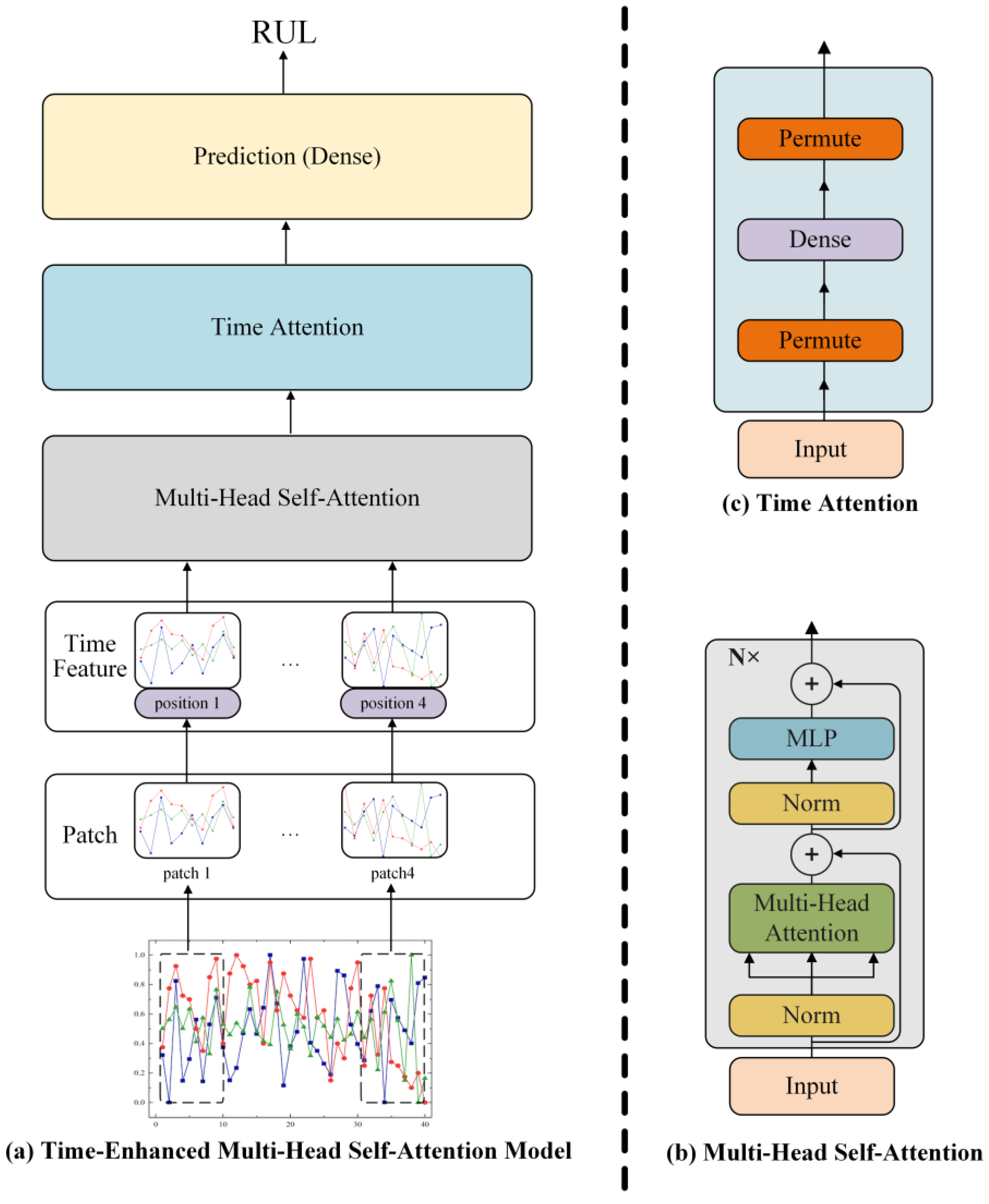
2.1. Time-Enhanced Multi-Head Self-Attention Model

A joint deep learning model combined with a multi-head self-attention (Transformer encoder) model and time-attention model was constructed to predict the RUL. Figure 1 illustrates the architectural design of the model. It is composed of five layers: the data time-division module, the time feature enhancement module, the multi-head self-attention module, the time-attention module, and the prediction module. This chapter introduces the modules involved in detail.

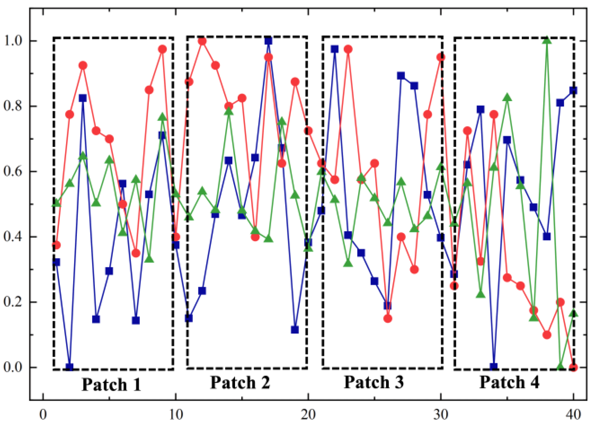
2.2. Data Time-Division Module

The standard Transformer encoder network’s input data are a group of text sequences. The prediction task presented in this paper was already a complete two-dimensional matrix with a time-series relationship. At the same time, to strengthen the continuous time-series relationship, we divided the input data with a time length of 40 into four patches with a time length of 10. This means that we treat each patch as a minimum unit, simply reshaping each patch into a one-dimensional vector to replace each word in natural language processing tasks. This can significantly lower the overall network’s computational complexity and better reflect key feature information. Additionally, it can reflect the time relationship within the patch. Figure 2 illustrates the division method.

2.3. Time Feature Enhancement Module

For the subsequent attention layer to better extract the time relationship between engine parameters and obtain relationship information between patches, this study added a position flag to reinforce the positional information between patches and to ensure that each patch contains both the engine parameter information for the current time period and the patch’s position (sequence) information. We also encoded the corresponding sequence information for each patch. The encoding equation is shown in Equation (1):

$$\begin{array}{c}P{E}_{\left(pos,2i\right)}=\sin \left(pos/10,{000}_{2i/d_{model}}\right)\\ P{E}_{\left(pos,2i+1\right)}=\cos \left(pos/10,{000}_{2i/d_{model}}\right)\end{array}$$

(1)

where pos represents the timing feature, and i represents the dimension, implying that each dimension of the timing feature corresponds to a sinusoid. The wavelengths form a geometric progression from 2π to 10,000·2π. This function enables the model to easily augment the temporal feature information with relative positions, since for any fixed offset K, $P{E}_{pos+K}$ can be represented as a linear function of $P{E}_{pos}$.

2.4. Multi-Head Self-Attention Module

The multi-head self-attention module is composed of the multi-head self-attention layer and the MLP layer. Multi-head self-attention can be interpreted as applying multiple self-attention models, collectively called the scaled dot-product attention function. The scaled dot-product attention function is a variant of attention. The input of this attention model is queried, keys of dimension $d_{k,}$ and values of dimension $d_v$. This attention model computes the dot products of the query with keys and divides the answer by $\sqrt{d_k}$. Finally, a SoftMax function is applied to obtain the weights of the values. The above values are integrated to obtain the publicity, as presented in Equation (2), where $d_k$ is the length of the input vector.

$$SelfAttention\left(Q,K,V\right)=\mathrm{softmax}\left(\frac{\mathrm{Q}{K}^T}{\sqrt{d_k}}\right)V$$

(2)

Figure 1 illustrates the multi-head self-attention layer. First we performed a layer norm operation on the whole patch before sending it to the multi-head self-attention layer. Then, we concatenated the outputs of the multi-head self-attention layer’s multiple attention functions. To calculate the attention function, the multi-head self-attention model maps a matrix with a larger dimension to a matrix with a smaller dimension, then splices and projects the results. The model architecture of the multi-head self-attention layer is shown in the lower half of subfigure (b) in Figure 1. Additionally, the equation is presented in Equation (3):

$$\begin{array}{c}MultiHead\left(Q,K,V\right)=Concat\left(hea{d}_1,···,hea{d}_h\right)W^O\\ hea{d}_i=Attention\left(Q{W}_i^Q,K{W}_i^K,V{W}_i^V\right)\end{array}$$

(3)

The MLP layer aims to obtain global timing feature information. The input of the MLP layer is its patch superimposed with the features information collected from the multi-head self-attention layer. This is then subjected to a layer norm operation, then supplied to a multi-layer perceptron for filtering and feature extraction. The model architecture of the MLP layer is shown in the upper half of subfigure (b) in Figure 1.

2.5. Time Attention Module

To predict the process of network layer feature extraction and accelerate the training process, we input the features that were extracted by the MLP layer perceptron screening and extraction into the attention layer. To start, we let the input pass through the Permute layer to invert the dimensions of the timing and MLP layer features. Then, using a fully connected layer and SoftMax, we calculated the weight of each timing feature and converted the dimension. Finally, we multiplied the input by the timing attention layer’s output value to achieve global time-point feature weighting. The subfigure (c) of Figure 1 illustrates the process.

2.6. Prediction Network Module

Unlike BERT [20] and other networks that added a special classification character to the data feature, the multi-head self-attention model is used to exchange information between different dimensions after collecting the time-attention layer’s features from the multi-head self-attention model. The extra classification features are employed in the final classification process. To ensure classification accuracy in the prediction task, this study chose to preserve more feature information and input it into the multi-layer perceptron to obtain the engine’s final life information.

2.7. Hyperparameter Selection

The benefit of deep learning for models is dependent on the parameters used in addition to the model itself. While there are usually minor differences in parameters while training the same model on different datasets, the manual parameter search is a somewhat ineffective strategy. The parameters were trained in this study using a parameter search library based on Bayesian optimisation. It is worth noting that, when some parameters were optimised in this study, the parameters were not properly selected (parameters other than the learning rate are presented in discrete numerical form). An algorithm used for automatic parameter selection, called Hyperopt [21], was used in this study to calculate the basic parameters of deep learning and the six hyperparameters (num head, d model, hidden layer, num layer, patch size, learning rate) in the network framework.

Table 1. Engine hyperparameter selection range table.

Hyperparameter	Range	Interval
patch size	[1, 10]	1
d model	[128, 1024]	64
hidden layer	[128, 2048]	64
num layer	[2, 4, 8]
num head	[2, 4, 8]
learning rate	[0.05, 0.02, 0.01, 0.005, 0.002, 0.001]

includes a list of these parameters.

3. Experiments

This section assesses our proposed method’s performance on aero-engine life prediction tasks and discusses the datasets, laboratory setup, parameter optimisation method, and assessment method used in our experiment. Finally, we analyse our experimental outcomes.

Our running environment for experimentation entails the following factors: The CPU of this experiment used Intel (R) Core (TM) i9-10900X. The memory was 96 G. The GPU used Nvidia GeForce RTX 3090. The environment for running was TensorFlow 2.4.0 + Python 3.8 + Win11.

3.1. Dataset Description

The dataset utilised in this study was NASA’s C-MAPSS engine degradation simulation dataset [22]. Each engine in this dataset contains data obtained from 21 sensors and three operational setup settings. This dataset classifies the entire dataset into four categories based on operational conditions and failure modes: FD001, FD002, FD003, and FD004. Figure 3 shows an example of three parameters of an engine (normalised data).

The dataset included a portion of the life cycle of multiple engines. Each engine is originally thought to be fairly healthy, but as the engine cycles through, the engine gradually wears out and eventually ceases to function. The data obtained from multiple engines formed the final dataset. The four datasets are listed in detail in

Table 2. The parameters of C-MAPSS datasets. Each dataset contains parameter information for multiple engines, from running to non-functioning.

C-MAPSS	FD001	FD002	FD003	FD004
Number of engines in training set	100	260	100	249
Number of engines in testing set	100	259	100	248
Operating conditions	1	6	1	6
Fault modes	1	1	2	2
Training set size	20,632	53,760	24,721	61,250
Testing set size	13,097	33,992	16,597	41,215

.

3.2. Data Preprocessing

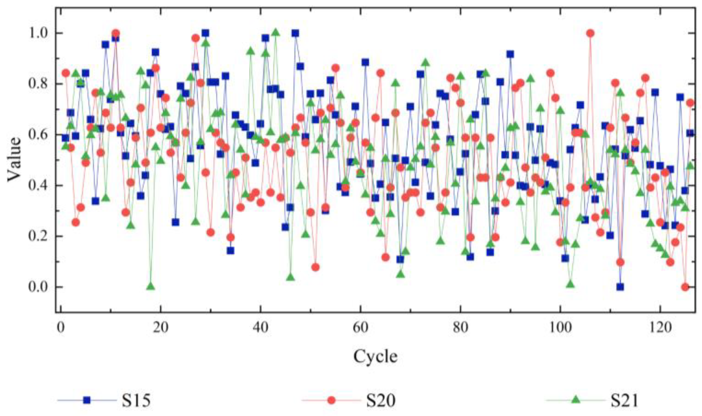
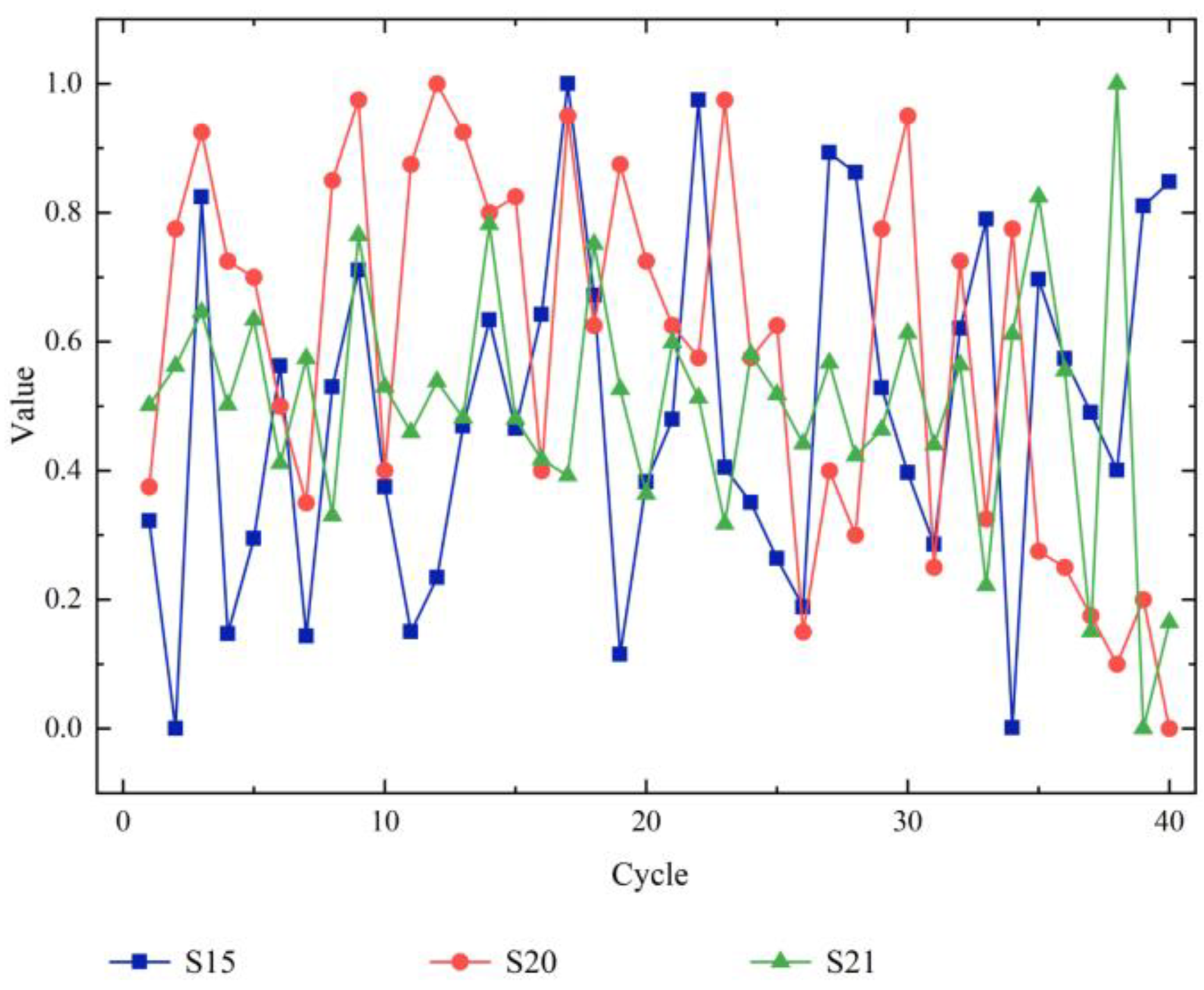
3.2.1. Feature Selection

We obtained improved data usability, simplified algorithms, and more easily understandable outcomes by reducing dimensionality and eliminating redundant or low-impact data. Finally, seventeen kinds of feature data were collected.

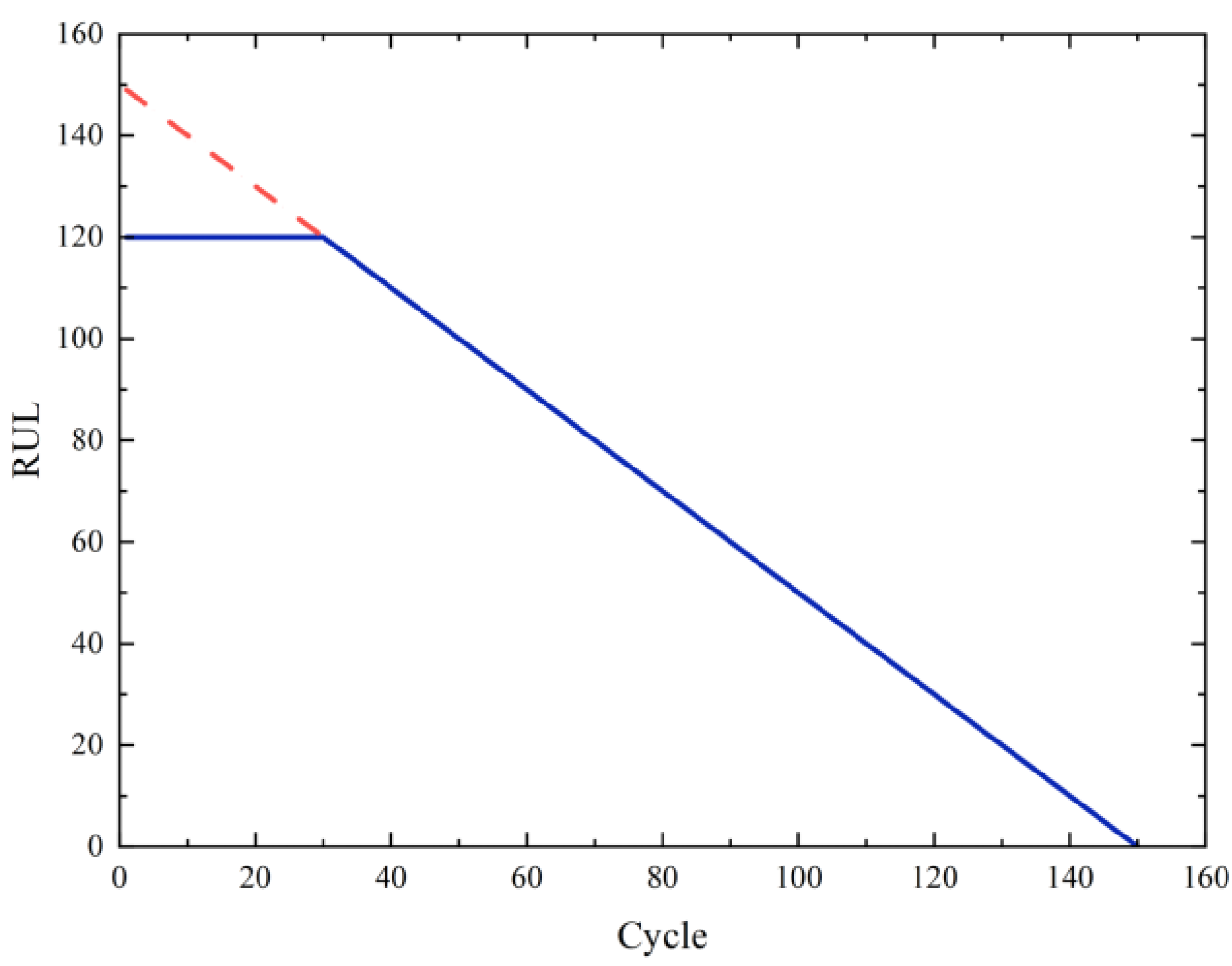
3.2.2. Calculating the Remaining Useful Life

The calculation for the RUL of the aircraft engine in the training set is shown in Equation (4). $Cycl{e}_{max}$ is the maximum number of operating cycles that each engine in the training set can achieve, and $Cycl{e}_{now}$ is the present number of operating cycles that each record can achieve.

$$RU{L}_{train}=Cycl{e}_{max}-Cycl{e}_{now},$$

(4)

Equation (5) shows the calculation of the RUL of the test set. The RUL is the engine’s actual RUL as documented in the RUL file. The $Cycl{e}_{max}$ is the maximum number of operating cycles that each engine has recorded in the test file, and $Cycl{e}_{now}$ is the current number of operating cycles associated with each record. The calculated RUL time correlates to the predicted label for each record. We observed that the longest engine running cycle in the training set was 362 cycles, the shortest was 128 cycles, and the average was 217 cycles; in the test set, the longest engine running cycle was 341 cycles, the shortest was 141 cycles, and the average was 218 cycles.

$$RU{L}_{test}=RUL+Cycl{e}_{max}-Cycl{e}_{now},$$

(5)

In reality, predicting the RUL of an aircraft engine based on its current operating parameters is difficult. Given that the data created by the long-term operation of the aero-engine are a long-time sequence and the engine’s performance is stable in the early phase of operation, the performance degradation is not evident. Due to a variety of factors, such as hardware wear and ageing during operation, the engine’s RUL reduces as the operation time grows. As illustrated in Figure 4, the piecewise linear degradation approach was employed to fit the connection between service time and remaining engine life. We obtained the number of cycles the engine continues to operate as the RUL and set a predetermined maximum RUL during the initial stages of engine operation.

3.2.3. Data Normalisation

Different features of data generally have distinct dimensions and dimensional units that affect the outcomes of unprocessed data analysis. To erase the dimensional influence between features, it is essential to normalise the data (normalisation processing) to scale different data to the same order of magnitude, allowing for a comprehensive comparative evaluation. Generally, there are two methods for data normalisation. The first is known as min–max normalisation, and the second is known as Z-score normalisation. Min–max normalisation was used to normalise the data in this study. The equation is as follows:

$$x^{\prime }=\frac{x-x_{min}}{x_{max}-x_{min}},$$

(6)

The preprocessing steps of data normalisation are data normalisation and the re-divide training set and the test set using the sliding time window. Specifically, the label of each window’s final data was used as the label for that window’s data, and the test set tests only the last window’s data.

3.2.4. Time Sliding Window

Time series data is vital to and prevalent in a wide variety of industries. Due to the high dimensionality and time-series characteristics of time series, direct training on the original data for regression prediction and other operations overlooks the short-term feature. This not only results in inefficient computing but also affects the algorithm’s accuracy and reliability. As a result, satisfactory results are impossible to achieve.

There are numerous approaches available to date for dealing with time series. The fixed-length sliding window is employed to cut and divide the original data for the aero-engine RUL prediction. By utilizing the divided sub-sequences data obtained for training prediction, one can effectively enhance the features of time-series data and improve the algorithm’s accuracy. The following are the specific algorithm steps. A time window with a time length of L and a sliding step size of S was selected based on the features of the time series; the first sliding window data were created by taking L pieces of original data from the first time point. Then, we moved the sliding window forward by the sliding step S along the time dimension to obtain the subsequent sliding window data. We repeated the previous step until the sliding window’s end reached the last original data. Finally, N groups of equal-scale sliding window data of size L*M are obtained.

At the same time, it was important for this paper to study the application of the attention model when the time window is regarded as the smallest unit. Therefore, in the choice of the time window length, the 40-step size commonly used in most papers was selected. As observed in Figure 5, the values of three sensors on the same engine are randomly chosen as raw data, and the sliding window slides forward along the time dimension with a fixed size. The size and meaning of the data training and test datasets after the time sliding window are shown in

Table 3. Size of dataset after sliding window.

Dataset	Train	Test
Input (simple num, window size, engine feature)	(11,631, 40, 21)	(96, 40, 21)
Output (simple num, RUL)	(11,631, 1)	(96, 1)

.

3.3. Optimisation Function

The preprocessed dataset was used to train the multi-head self-attention model with the Adam optimiser as the model’s optimiser function. Adam [23] is a method for dynamically adjusting the learning rate of each parameter. It combines the advantages of RMSprop and AdaGrad optimisation methods and employs gradient first- and second-order matrix estimates. This method provides several significant advantages over more typical random optimisation algorithms, such as Gradient Descent (SGD). Additionally, in many circumstances, the default optimiser is excellent. The Adam optimiser’s default parameters were utilised for training in this study.

3.4. Performance Evaluation Index

To assure the model’s successful overall performance, we evaluated our model and the comparative model by adopting three different performance metrics. The following factors are the detailed definitions and equations used for the two models:

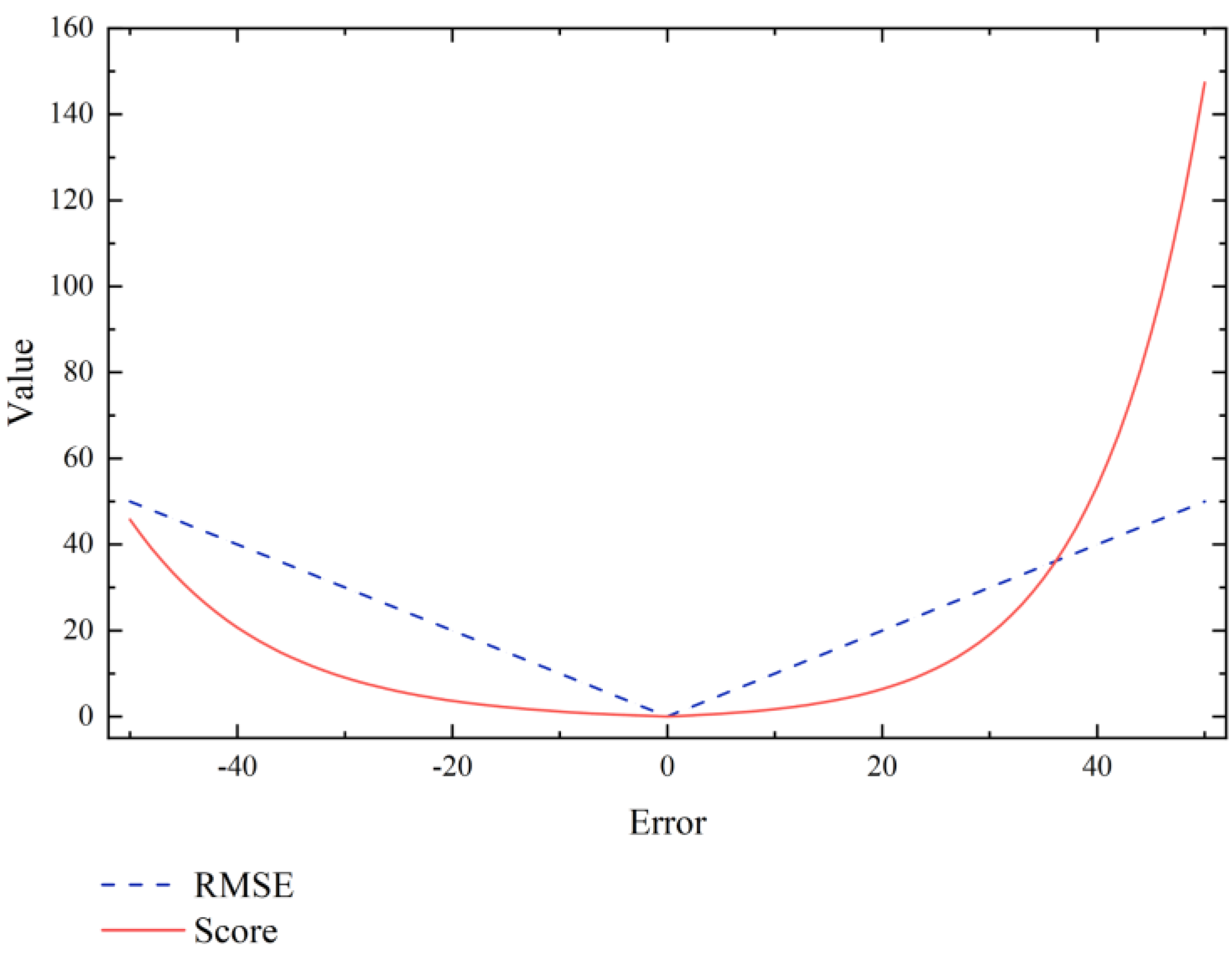
• The Root Mean Square Error (RMSE) was used to evaluate the experiment’s performance. The Root Mean Square Error (RMSE) is a frequently used performance metric for evaluating regression prediction models. It is equal to the square of the deviation and the square of the ratio of the predicted and actual values. It is used to quantify the deviation between predicted and observed values. The lower the deviation between the predicted and actual values, the more accurate the prediction model. The equation for the RMSE is as follows:

$$RMSE=\sqrt{\frac{1}{n}{\displaystyle \sum }_{i=1}^n{\left(y_i-\widehat{y}\right)}^2}$$

(7)

In the above equation, n represents the total number of predicted samples, y represents the true value of each sample, and $\widehat{y}$ represents the predicted value of each sample.

2.

When predicting the RUL of an aero-engine, there are two possible outcomes: the predicted RUL is less than the actual RUL, or the predicted RUL is greater than the actual RUL. In both circumstances, the approach used by RMSE bears the same penalty. In practice, however, the underestimated RUL prediction benefits from having an early warning signal, hence decreasing the probability of fatalities caused due to engine damage. As a result, the scoring index score is proposed in Equation (8). The cost of an overestimated RUL prediction, on the other hand, is significantly higher than the cost of an underestimated one. This method is more practical and enables a more accurate evaluation of the model prediction effect.

$$Score=\{\begin{array}{c}{\displaystyle {\displaystyle \sum }_{i=1}^n}\left(e^{-\left(\frac{\left({\widehat{y}}_i-y_i\right)}{13}\right)}-1\right) , \left({\widehat{y}}_i-y_i\right)<0\\ {\displaystyle {\displaystyle \sum }_{i=1}^n}\left(e^{\left(\frac{\left({\widehat{y}}_i-y_i\right)}{10}\right)}-1\right) , \left({\widehat{y}}_i-y_i\right)>0\end{array}$$

(8)

A comparison of the metrics is shown in Figure 6.

4. Results

We evaluated our proposed model using the RMSE and score evaluation functions, compared it to other existing models, and further analysed the results in this section.

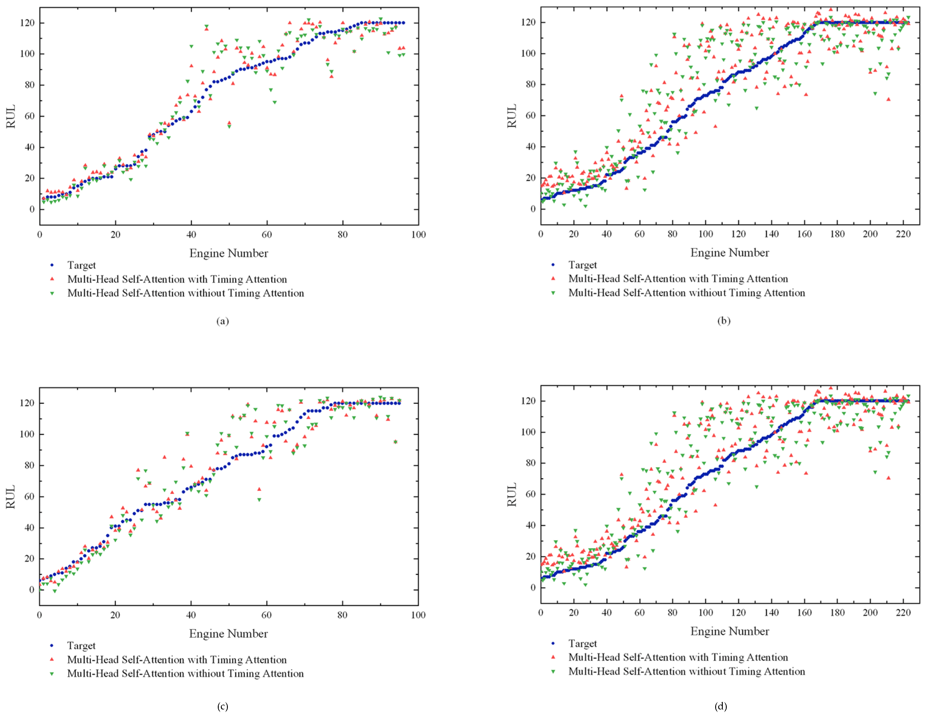
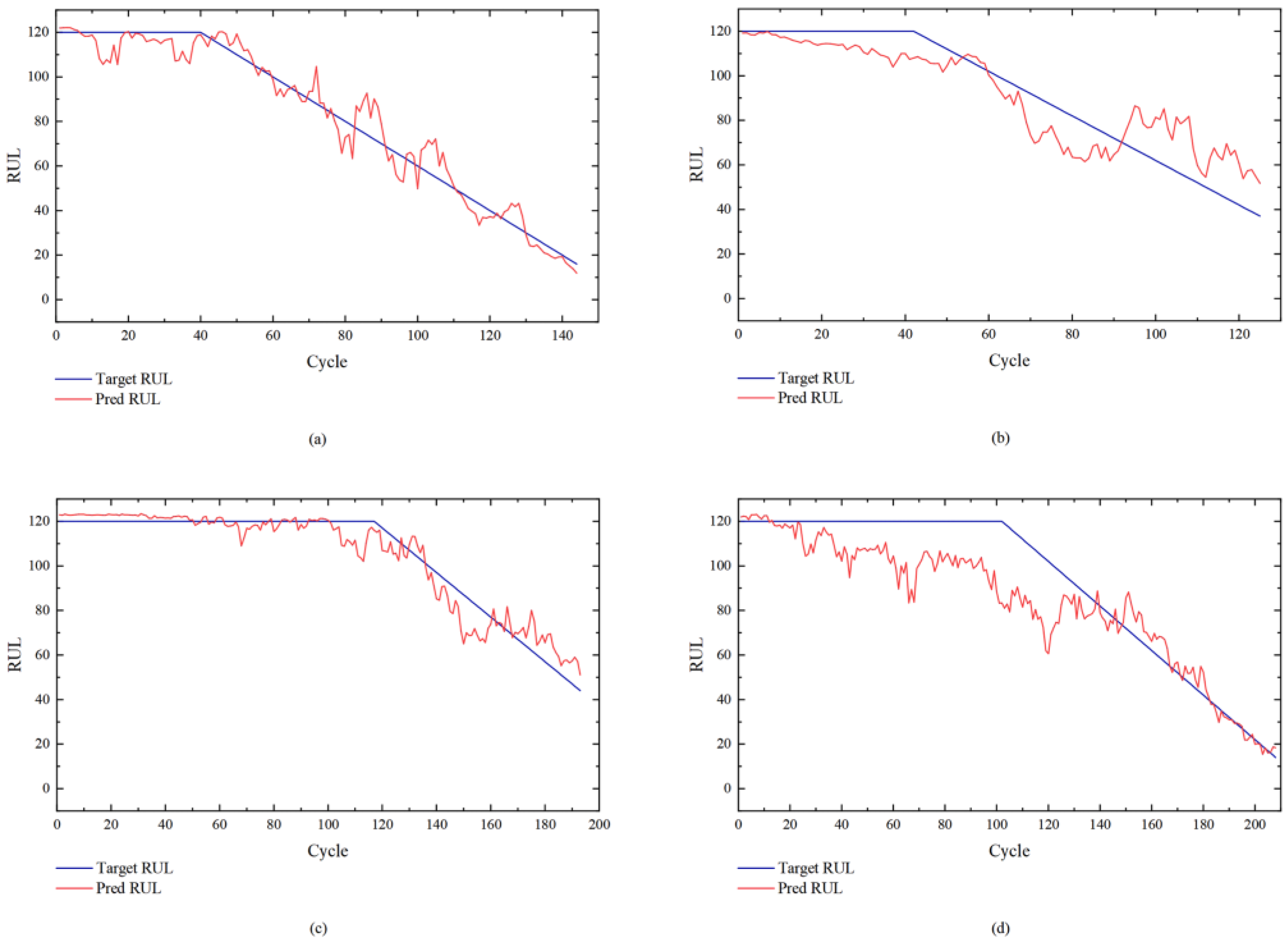
4.1. Experimental Results

Figure 7 depicts the experimental results of the proposed model on the CMAPSS dataset. Figure 7 illustrates the prediction outcomes of sub-datasets under diverse operation settings (for the convenience of observation, we sorted the remaining lifetimes observed from high to low). As indicated in Figure 7, the remaining service life prediction results for a single engine are not desirable. This may be because, although the dataset offers a high number of parameters, the relationship between the parameters and the degradation characteristics is unclear or the overall parameter values are very little. It is evident that the algorithm model provided in this study is vastly superior when the remaining service life of the engine is short. This could be because the engine’s parameters did not considerably alter throughout the early degradation period. Hence, this demonstrates that the model proposed in this study has the potential to effectively perform preventive tasks. In other words, the model can effectively provide pertinent recommendations when engine failure is imminent.

As a supplementary display, we extracted the prediction results of a single engine from each sub-dataset in Figure 8. Figure 8 demonstrates that when the result for a single engine is close to the critical value, the prediction effect is frequently greater than it was at the beginning of the degradation process. This partially supports the study’s results.

Combining Figure 6 and Figure 7, it is evident that the predictive effect of the FD001 and FD003 datasets are considerably greater than that of the FD002 and FD004 datasets. Considering the operating environment and fault state of the engine, we can conclude that the engine has an impact on the remaining service-life prediction. Specifically, FD001 is the strongest predictor because of its single working condition and single failure mode, whereas FD004 is the weakest predictor due to its 6 working conditions and 2 failure modes. Table 2 displays the operating conditions and failure modes for each dataset.

4.2. Comparison with Previous Work

Our proposed model is available in two variants, one with an attention model (with attention) and one without (no attention). We used the RMSE and score evaluation indicators to compare these models with many previous works on the C-MAPSS dataset; the best results are marked in bold.

Our paper compared the results to the best results in each subset and presented the percentage improvement of the results. As observed in

Table 4. Performance comparison between related methods and our proposed model on the C-MAPSS datasets. The evaluation function is the score.

C-MAPSS	YEAR	FD001	FD002	FD003	FD004
ConvJANET E-D [24]	2018	262.71	1401.95	333.79	2282.23
HDNN [25]	2019	245.00	1282.42	287.72	1527.42
BiLSTM + ED [26]	2019	273.00	3099.00	574.00	3202.00
RBM + LSTM [27]	2019	231.00	3366.00	251.00	2480.00
MS-DCNN [28]	2020	196.22	3747.00	241.89	2257.27
DA-CNN [29]	2020	229.48	1842.38	257.11	2317.32
RBPF [30]	2020	383.39	1226.97	375.29	2071.51
Attention Bidirectional LSTM [31]	2021	473	1223	676	2684
DCNN-LightGBM [32]	2021	232.0	-	277.8	-
KGHM [33]	2022	250.99	1131.03	333.44	3356.10
Double Attention-based Architecture [18]	2022	198	1575	290	1741
Transformer Encoder	2022	272.17	1045.70	228.92	2277.16
Transformer Encoder + Attention (this paper)	2022	183.75	1008.08	219.63	1751.23
Compare with State of the Art		+6.36%	+3.40%	+4.06%	−14.60%

and

Table 5. Performance comparison between related methods and our proposed model on the C-MAPSS datasets. The evaluation function is RMSE.

C-MAPSS	YEAR	FD001	FD002	FD003	FD004
ConvJANET E-D [24]	2018	12.67	16.19	12.80	19.15
HDNN [25]	2019	13.02	15.24	12.22	18.15
BiLSTM + ED [26]	2019	14.47	22.07	17.48	23.49
RBM + LSTM [27]	2019	12.56	22.73	12.10	22.66
MS-DCNN [28]	2020	11.44	19.35	11.67	22.22
DA-CNN [29]	2020	11.78	16.95	11.56	18.23
RBPF [30]	2020	15.94	17.15	16.17	20.72
Attention Bidirectional LSTM [31]	2021	15.87	16.59	15.10	14.36
GCU-Transformer [19]	2021	11.27	22.81	11.42	24.86
DCNN-LightGBM [32]	2021	12.79	-	13.21	-
KGHM [33]	2022	13.18	13.25	13.54	19.96
Double Attention-based Architecture [18]	2022	12.25	17.08	13.39	19.86
Transformer Encoder	2022	12.05	16.72	11.82	18.27
Transformer Encoder + Attention (this paper)	2022	10.35	15.82	11.34	17.35
Compare with State of the Art		+8.16%	−3.80%	+0.70%	−20.82%

, the models suggested in this study establish a commanding lead in the FD001 and FD003 datasets. However, only a few metrics in the FD002 and FD004 datasets produce superior outcomes. This may be because the FD002 and FD004 datasets work under more complex fault working conditions than the FD001 and FD003 datasets. Overall, our model performed well in simple working modes and was above average in complex situations. At the same time, the focus of this paper was mainly on discussing the extent to which attention models can be applied to the prediction task in this field, and we did not modify the fundamental network architecture for the task environment of engine-life prediction. This implies that the pure attention model has good performance in solving time-series problems, but adjustment for the problem is also essential. While our model shows good performance, there is a great deal of room for improvement.

5. Conclusions and Future Prospects

We presented a model for the engines’ RUL timing prediction in this study that was entirely based on the mechanism. On the C-MAPSS dataset, the model we proposed showed its superiority. In comparison to convolutional neural networks, recurrent neural networks, and their variants, the multi-head self-attention model is more efficient at extracting correlations from time-series data. Additionally, for time-series-related problems, effective information can be extracted and analysed with better accuracy and at a more rapid speed for related tasks after the addition of a time-attention model. The proposed multi-head self-attention model minimises model overestimation while enhancing overall fitting, potentially lowering the possibility of an accident caused by engine damage in actual applications.

Some deficiencies could be addressed further in future studies. First, our approach did not significantly improve in difficult circumstances. We believe that for the engine there is an exclusive network capable of processing the relevant data. Moreover, how to further enhance the model’s performance for time-series data is a topic worthy of discussion and exploration. In addition, because many applications and research directions have shifted in the research, the majority of research directions that apply the network to the RUL task are more concerned with reducing the network’s weight, while this study did not evaluate the relevant direction. Lastly, the optimisation of the model would be another intriguing topic for future research.

References

1. Wang, D.; Tsui, K.-L.; Miao, Q. Prognostics and health management: A review of vibration based bearing and gear health indicators. IEEE Access 2017, 6, 665–676. [Google Scholar] [CrossRef]
2. Pecht, M.G. A prognostics and health management roadmap for information and electronics-rich systems. IEICE ESS Fundam. Rev. 2009, 3, 25–32. [Google Scholar] [CrossRef] [Green Version]
3. Lau, D.; Fong, B. Special issue on prognostics and health management. Microelectron. Reliab. 2011, 2, 253–254. [Google Scholar] [CrossRef]
4. Bahdanau, D.; Cho, K.; Bengio, Y. Neural machine translation by jointly learning to align and translate. arXiv 2014, arXiv:1409.0473. [Google Scholar]
5. Saufi, M.S.R.M.; Hassan, K.A. Remaining useful life prediction using an integrated Laplacian-LSTM network on machinery components. Appl. Soft Comput. 2021, 112, 107817. [Google Scholar] [CrossRef]
6. Ahn, G.; Yun, H.; Hur, S.; Lim, S. A Time-Series Data Generation Method to Predict Remaining Useful Life. Processes 2021, 9, 1115. [Google Scholar] [CrossRef]
7. Fan, J.; Yung, K.C.; Pecht, M. Physics-of-failure-based prognostics and health management for high-power white light-emitting diode lighting. IEEE Trans. Device Mater. Reliab. 2011, 11, 407–416. [Google Scholar] [CrossRef]
8. Miao, J.; Li, X.; Ye, J. Predicting research of mechanical gyroscope life based on wavelet support vector. In Proceedings of the 2015 First International Conference on Reliability Systems Engineering (ICRSE), Beijing, China, 21–23 October 2015. [Google Scholar]
9. Nieto, P.G.; García-Gonzalo, E.; Lasheras, F.S.; de Cos Juez, F.J. Hybrid PSO–SVM-based method for forecasting of the remaining useful life for aircraft engines and evaluation of its reliability. Reliab. Eng. Syst. Saf. 2015, 138, 219–231. [Google Scholar] [CrossRef]
10. Galar, D.; Kumar, U.; Fuqing, Y. RUL prediction using moving trajectories between SVM hyper planes. In Proceedings of the 2012 Annual Reliability and Maintainability Symposium, Reno, Nevada, 23–26 January 2012. [Google Scholar]
11. Zhang, Y.; Xiong, R.; He, H.; Pecht, M.G. Long short-term memory recurrent neural network for remaining useful life prediction of lithium-ion batteries. IEEE Trans. Veh. Technol. 2018, 67, 5695–5705. [Google Scholar] [CrossRef]
12. Lin, Y.; Koprinska, I.; Rana, M. Temporal convolutional attention neural networks for time series forecasting. In Proceedings of the 2021 International Joint Conference on Neural Networks (IJCNN), Shenzhen, China, 18–23 July 2021. [Google Scholar]
13. Qin, Y.; Song, D.; Chen, H.; Cheng, W.; Jiang, G.; Cottrell, G. A dual-stage attention-based recurrent neural network for time series prediction. arXiv 2017, arXiv:1704.02971. [Google Scholar]
14. Li, X.; Ding, Q.; Sun, J.Q. Remaining useful life estimation in prognostics using deep convolution neural networks. Reliab. Eng. Syst. Saf. 2018, 172, 1–11. [Google Scholar] [CrossRef] [Green Version]
15. Sateesh Babu, G.; Zhao, P.; Li, X.L. Deep convolutional neural network based regression approach for estimation of remaining useful life. In Proceedings of the International Conference on Database Systems for Advanced Applications, Dallas, TX, USA, 16–19 April 2016. [Google Scholar]
16. Xu, K.; Ba, J.; Kiros, R.; Cho, K.; Courville, A.; Salakhudinov, R.; Zemel, R.; Bengio, Y. Show, attend and tell: Neural image caption generation with visual attention. In Proceedings of the International Conference on Machine Learning, PMLR, Lille, France, 7–9 July 2015. [Google Scholar]
17. Dosovitskiy, A.; Beyer, L.; Kolesnikov, A.; Weissenborn, D.; Zhai, X.; Unterthiner, T.; Dehghani, M.; Minderer, M.; Heigold, G.; Gelly, S.; et al. An image is worth 16 × 16 words: Transformers for image recognition at scale. arXiv 2020, arXiv:2010.11929. [Google Scholar]
18. Liu, L.; Song, X.; Zhou, Z. Aircraft engine remaining useful life estimation via a double attention-based data-driven architecture. Reliab. Eng. Syst. Saf. 2022, 221, 108330. [Google Scholar] [CrossRef]
19. Mo, Y.; Wu, Q.; Li, X.; Huang, B. Remaining useful life estimation via transformer encoder enhanced by a gated convolutional unit. J. Intell. Manuf. 2021, 32, 1997–2006. [Google Scholar] [CrossRef]
20. Devlin, J.; Chang, M.W.; Lee, K.; Toutanova, K. Bert: Pre-training of deep bidirectional transformers for language understanding. arXiv 2018, arXiv:1810.04805. [Google Scholar]
21. Bergstra, J.; Yamins, D.; Cox, D. Making a science of model search: Hyperparameter optimization in hundreds of dimensions for vision architectures. In Proceedings of the International Conference on Machine Learning, PMLR, Atlanta, GA, USA, 17–19 June 2013. [Google Scholar]
22. Saxena, A.; Goebel, K. Turbofan Engine Degradation Simulation Dataset; NASA Ames Research Center: Moffett Field, CA, USA, 2008; pp. 1551–3203. [Google Scholar]
23. Kingma, D.P.; Ba, J. Adam: A method for stochastic optimization. arXiv 2014, arXiv:1412.6980. [Google Scholar]
24. Astorga, N.O. Convolutional Recurrent Neural Networks for Remaining Useful Life Prediction in Mechanical Systems. Bachelor’s Thesis, Universidad de Chile, Santiago, Chile, 2018. [Google Scholar]
25. Al-Dulaimi, A.; Zabihi, S.; Asif, A.; Mohammadi, A. Hybrid deep neural network model for remaining useful life estimation. In Proceedings of the ICASSP 2019 IEEE International Conference on Acoustics, Speech and Signal Processing (ICASSP), Brighton, UK, 12–17 May 2019. [Google Scholar]
26. Yu, W.; Kim, I.Y.; Mechefske, C. Remaining useful life estimation using a bidirectional recurrent neural network based autoencoder scheme. Mech. Syst. Signal Process. 2019, 129, 764–780. [Google Scholar] [CrossRef]
27. Ellefsen, A.L.; Bjørlykhaug, E.; Æsøy, V.; Ushakov, S.; Zhang, H. Remaining useful life predictions for turbofan engine degradation using semi-supervised deep architecture. Reliab. Eng. Syst. Saf. 2019, 183, 240–251. [Google Scholar] [CrossRef]
28. Li, H.; Zhao, W.; Zhang, Y.; Zio, E. Remaining useful life prediction using multi-scale deep convolutional neural network. Appl. Soft Comput. 2020, 89, 106113. [Google Scholar] [CrossRef]
29. Song, Y.; Gao, S.; Li, Y.; Jia, L.; Li, Q.; Pang, F. Distributed attention-based temporal convolutional network for remaining useful life prediction. IEEE Internet Things J. 2020, 8, 9594–9602. [Google Scholar] [CrossRef]
30. Cai, H.; Feng, J.; Li, W.; Hsu, Y.M.; Lee, J. Similarity-based particle filter for remaining useful life prediction with enhanced performance. Appl. Soft Comput. 2020, 94, 106474. [Google Scholar] [CrossRef]
31. Shah, S.R.B.; Chadha, G.S.; Schwung, A.; Ding, S.X. A Sequence-to-Sequence Approach for Remaining Useful Lifetime Estimation Using Attention-Augmented Bidirectional LSTM. Intell. Syst. Appl. 2021, 10, 200049. [Google Scholar] [CrossRef]
32. Liu, L.; Wang, L.; Yu, Z. Remaining Useful Life Estimation of Aircraft Engines Based on Deep Convolution Neural Network and LightGBM Combination Model. Int. J. Comput. Intell. Syst. 2021, 14, 165. [Google Scholar] [CrossRef]
33. Li, Y.; Chen, Y.; Hu, Z.; Zhang, H. Remaining useful life prediction of aero-engine enabled by fusing knowledge and deep learning models. Reliab. Eng. Syst. Saf. 2023, 229, 108869. [Google Scholar] [CrossRef]
Figure 1. Frame diagram of multi-head self-attention and remaining useful life prediction models.
Aerospace 10 00080 g001
Figure 2. Time window serialisation.
Aerospace 10 00080 g002
Figure 3. Data sample for a single engine.
Aerospace 10 00080 g003
Figure 4. Schematic diagram of segmented linear degradation.
Aerospace 10 00080 g004
Figure 5. Sliding time window. Time window serialisation.
Aerospace 10 00080 g005
Figure 6. Comparison of the RMSE and score.
Aerospace 10 00080 g006
Figure 7. Comparison between the target and predicted RUL for test units. (a) FD001 test set. (b) FD002 test set. (c) FD003 test set. (d) FD004 test set.
Aerospace 10 00080 g007
Figure 8. RUL predictions of units belonging to different subsets. (a) Unit 19 in FD001. (b) Unit 15 in FD002. (c) Unit 1 in FD003. (d) Unit 8 in FD004.
Aerospace 10 00080 g008