1. Introduction
The aeroengine requires safe and reliable operation during the service period. However, as a complex aerodynamic system, aeroengine performance degradation will inevitably occur if it works under harsh conditions of high temperature, high pressure and high speed for a long time [
1]. At the same time, rapid changes in aeroengine operating conditions accelerate the degradation process and even the risk of fault and invalidity [
2]. At present, researchers mainly monitor, track and control the aeroengine status by collecting airborne sensor data of the aeroengine and analyze the degree of performance degradation for fault diagnosis to help formulate maintenance plans and improve flight safety [
3,
4]. The core content of the aeroengine gas path performance fault diagnosis is used to judge the performance degradation or fault condition of engine gas path components (compressor, turbine, etc.) or the overall engine through the deviation between the actual value of engine state parameters and the standard value under the healthy state [
5]. The state parameters are the parameters used to characterize the engine performance, while the
EGT of the engine is a key indicator to reflect the overall performance of the engine, and it is the key index of engine maintenance for airlines. The control parameters are relevant parameters that affect the engine state parameters [
6]. The baseline of the aeroengine is characterized as a nonlinear functional relationship between the state parameters and control parameters of the same engine fleet and model in a healthy, steady state. The deviation of the engine
EGT depends on the accuracy of the actual measurements and the engine
EGT baseline model. Accurate prediction of engine
EGT is essential to maintain engine operation, and an accurate engine
EGT baseline model is the basis of engine gas path performance monitoring and fault diagnosis. Therefore, accurate and reliable engine
EGT baseline modeling method is required [
7].
Baseline modeling of gas path state parameters of the aeroengine is mainly divided into two methods: model-based modeling and data-driven modeling. The physical model-based method builds a high-precision mechanical model based on aero-thermodynamic theory and engine operating characteristics without historical experience. Haglind and Elmegaard [
8] developed two models for predicting engine part–load performance, which can well predict exhaust temperatures. Song et al. [
9]. developed an engine performance prediction model and verified the accuracy of the model in predicting engine gas path state parameters. Sangjo et al. [
10]. proposed a modeling method in engine transient mode for the prediction of engine gas path state parameters. However, these methods require a complete engine component characteristic map, and complex modeling processes limit the computational performance and applicability [
11].
Data-driven methods do not require complex theory models but make full use of experience and knowledge in relevant fields to build state parameters and control parameters-related models based on actual measured data. Data-driven methods need to extract features from non-linear, high-dimensional sample data firstly. However, in practice, engine performance is affected by many parameters, which present complex non-linear relationships. Establishing an engine baseline model is a typical regression prediction problem which extracts non-linear characteristics from high-dimensional data. In recent years, with the development of machine learning and the progress of sensor technology, the data-driven baseline prediction of engine state parameters has attracted wide attention from academia and industry [
12]. Artificial neural network (ANN), as a powerful proxy model, has been widely used in engine state parameter baseline prediction [
13]. Nikpey et al. [
14,
15] developed an ANN model for micro-engines that can predict engine state parameters with high accuracy. Rua et al. [
16] developed a state parameter prediction model for an external combustion engine with ANN for thermal diagnosis of the engine. Yildirim et al. [
17] used polynomial regression to determine the input parameters of the model and used them as ANN inputs to establish the baseline model of engine state parameters. Yu Y et al. [
18] established the aeroengine
EGT baseline model by combining the kernel principal component analysis (KPCA) with the deep trust network (DBN). Omer Osman Dursun et al. [
19] predicted
EGT of the conceptual turboprop engine (C-TPE) by using artificial neural networks (ANN) and short and long-term memory (LSTM) methods. Although the neural network has a strong nonlinear fitting ability, it is prone to problems of divergence and low accuracy when the training sample set is small. In addition, other machine learning algorithms, such as support vector regression (SVR) [
20], extreme learning machine [
21,
22], regression tree [
23], and multivariate linear regression [
24,
25], have received extensive attention in the data-driven field. However, any machine learning algorithm has its limitations, and no algorithm can be perfectly applied to all tasks. Due to the diversity of engine flight data, on which the machine learning model has the highest prediction accuracy, the best calculation efficiency and strong applicability still need to be analyzed in detail.
Accurate monitoring and prediction of aeroengine performance is the core content of the aeroengine health management system. Aeroengine EGT is the key index for airlines to maintain engines. In order to obtain an accurate and reliable engine EGT baseline model, four aeroengine EGT baseline prediction frameworks based on machine learning are developed in this paper. Due to intense varying operating conditions of the aeroengine, noise exists in the data collected by sensors. Previous studies rarely considered the impact of measurement noise on baseline prediction, which may affect the accuracy of the baseline model. In order to eliminate the effect of noise on the accuracy of the baseline model as much as possible, the unscented Kalman filter (UKF) is used for data noise reduction. The original data was pre-processed, the correlation between each variable and EGT was analyzed, the engine EGTOEM value in ACARS flight data was taken as the target output and the extracted data features were input into the baseline models for forecasting. Four different machine learning algorithms were used to develop the engine baseline model in this paper, including the Generalized Regression Neural Network (GRNN), Radial Basis Function Neural Network (RBF), Support Vector Regression (SVR) and Random Forest (RF). At the same time, the performance of the four machine learning models was evaluated from the three aspects of training accuracy, prediction stability and calculation time. In this paper, the methodologies are designed not only to obtain high-precision EGT baseline models but also to ensure applicability of prediction frameworks.
2. Methodology
As the core of artificial intelligence, machine learning is specialized in studying how computers simulate or realize human learning behavior. It mainly uses induction and synthesis to obtain new knowledge or skills and reorganizes existing knowledge structures to continuously improve its own performance. Its applications cover all fields. Machine learning includes basic concepts such as instances, features, labels, feature vectors and datasets—where an instance is a data sample that describes an item or object, a feature represents the attribute of an instance, a label represents the required value or category of an instance, a feature vector represents a collection of all features associated with an instance and a data set is a collection of instances. The feature vector is usually represented as follows:
In the formula,
X represents the feature vector value,
d is the dimension of the eigenvector and
Y represents the label of the instance. The dataset containing
n instances can be represented as:
Baseline exhaust gas temperature prediction for the aeroengine based on data-driven methods belongs to supervised learning in machine learning. The task of supervised learning is to learn a model from the dataset of multiple instances and use the model to predict the Y of all unknown instances. Supervised learning relies on a large number of instance datasets and optimizes some super parameters by minimizing the objective function to obtain the required accuracy in the iterative process. The dataset is usually divided into the training set and the test set, namely, the training sample and the test sample. The instance samples in the training set are used to train the model, and the instance samples in the test set are used to evaluate the generalization performance of the model. These machine learning methods are briefly described in the following sections.
2.1. The GRNN
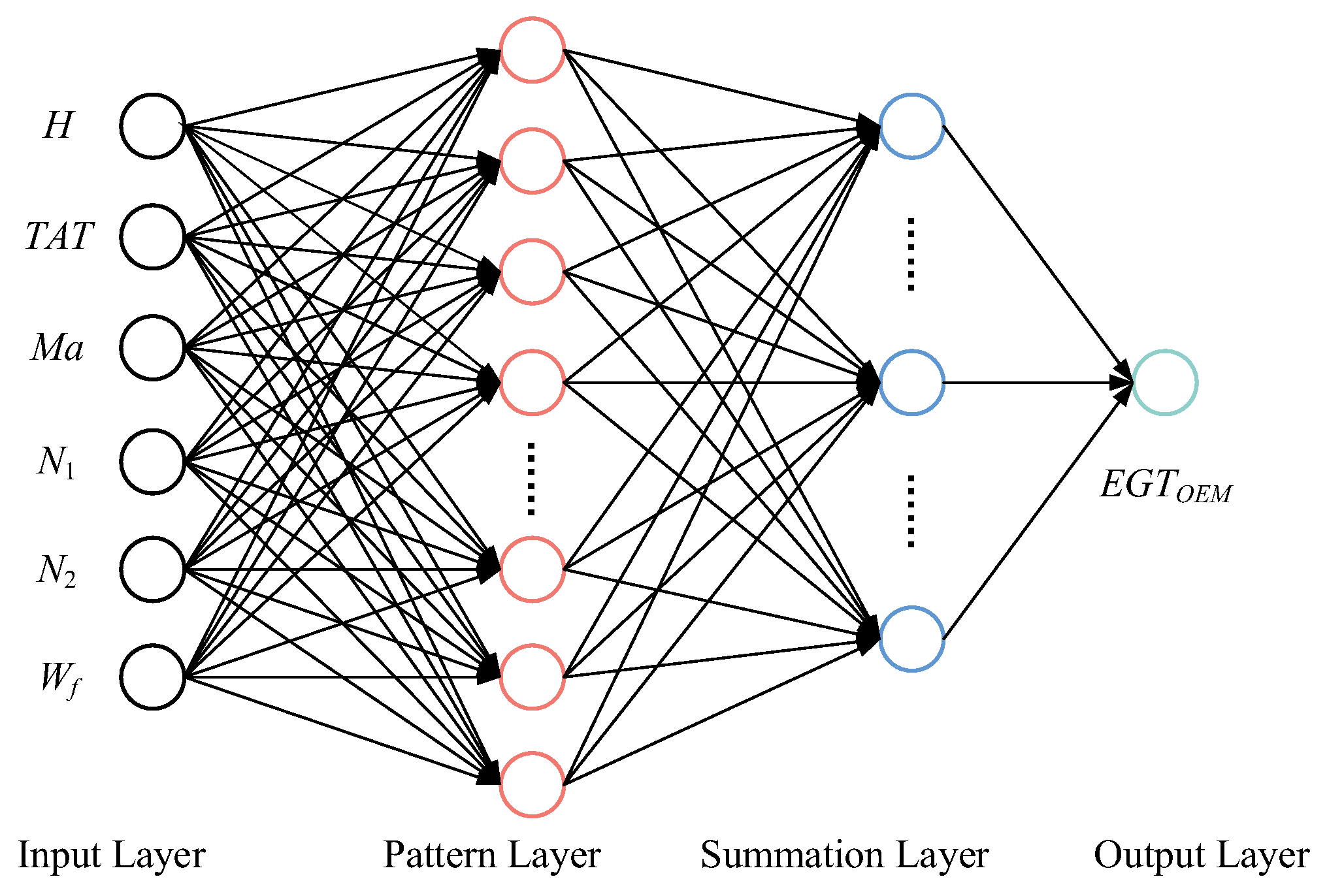
The network structure of the generalized regression neural network (GRNN) is shown in
Figure 1. The whole network consists of four layers of neurons: the first layer is the input layer of the GRNN; the number of neurons in the input layer is the same as the dimension of the input vector in the learning sample and the second layer is the pattern layer of the GRNN. The number of neurons in the pattern layer is equal to the number of learning samples
n. Each neuron corresponds to different samples. The third layer is the summation layer of the GRNN, in which two types of neurons are used for summation. The fourth layer is the output layer of the GRNN. The number of neurons in the output layer is equal to the dimension of the output vector in the learning sample [
26].
In the research of this paper, the GRNN is based on nonparametric nuclear regression, takes sample data as the verification condition of the posterior probability and carries out nonparametric estimation. Finally, the correlation density function between the dependent variable and independent variable in the GRNN is calculated from training samples, and the relative independent variable’s return value of the dependent variable is calculated. The parameter setting of the GRNN is convenient. The whole neural network can adjust the performance of the GRNN only by setting the smoothing factor in the GRNN’s core function [
27]. Where the joint probability density function of two random variables
x and
y in GRNN is assumed to be
f(
x,
y) and the observed sample of
x is
X, then the conditional mean is:
The unknown probability density function
f(
x,
y) can be obtained from the nonparametric estimates of the observed samples of
x and
y:
where
Xi and
Yi represent the observed values of
x and
y, respectively.
δ represents the smoothing factor;
n represents the number of samples, and
d represents the dimension of
x. From Equations (3) and (4):
Formula (5) represents the output of the network. The errors of the GRNN’s output data and training samples are mainly determined by the smoothing factor. By adjusting the smoothing factor, better performance can be obtained without iterative training, such as the traditional neural network. Compared with the traditional neural network, The GRNN has higher approximation accuracy and faster training speed and is not prone to local minimal problems.
2.2. The RBF
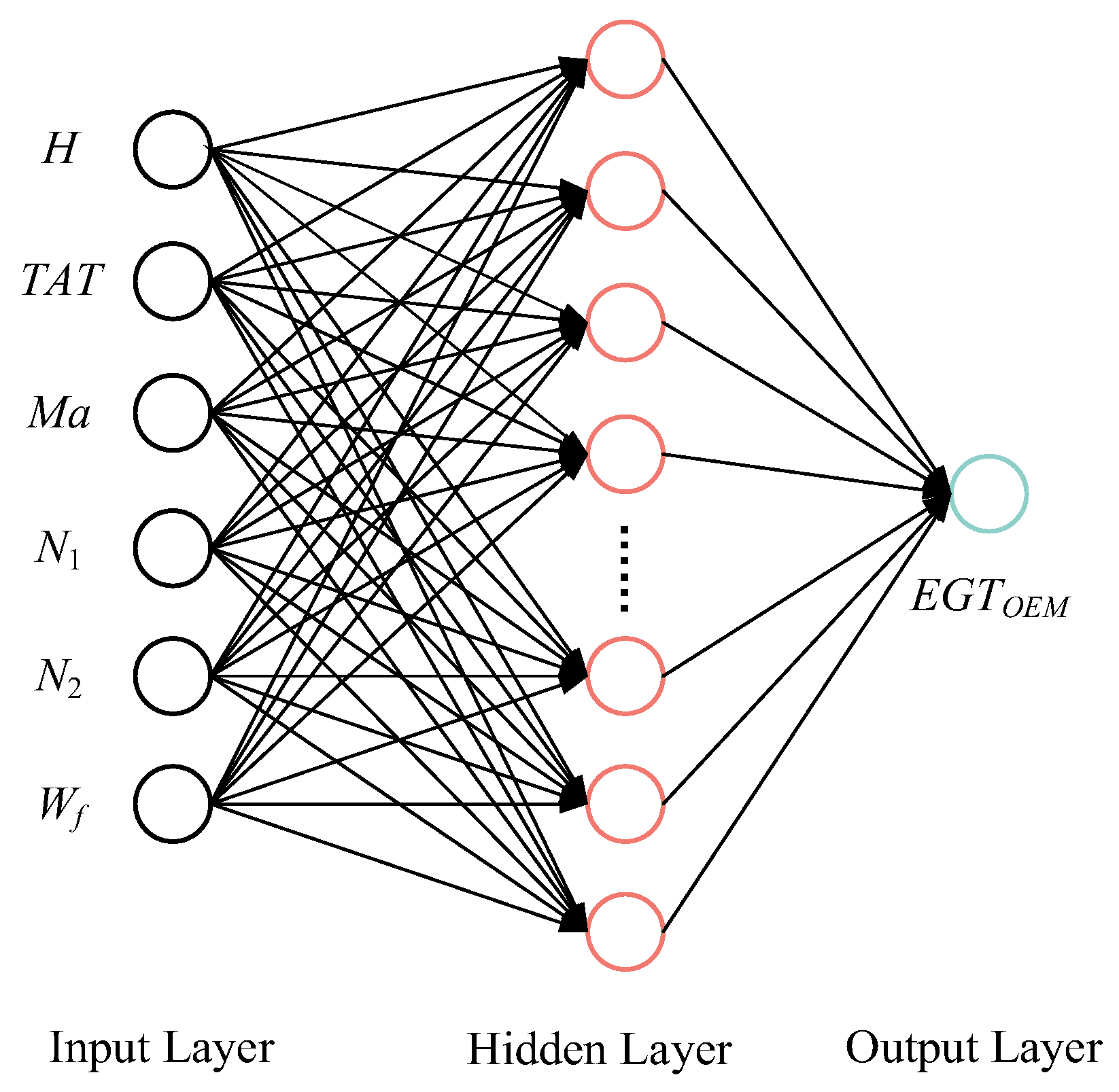
Radial Basis Function (RBF) network is a network with a simple structure and fast convergence speed that can approximate any nonlinear function. The RBF network has a good performance of uniform approximation to a nonlinear network and has been widely used in different industries and fields. The network structure of the RBF is shown in
Figure 2, which is a forward network composed of three layers: the first layer is the input layer, and the number of nodes is equal to the dimension of the input; the second layer is the hidden layer, and the number of nodes depends on the complexity of the problem; and the third layer is the output layer, and the number of nodes is equal to the dimension of the output data [
28].
Assuming that the input is a
d-dimensional vector
x and the output is a real value, the RBF network can be expressed as:
where
q is the number of hidden layer neurons,
ci and
wi are the corresponding centers and weights of the
i-th hidden layer neurons, respectively, and
ρ is the radial basis function. In this paper, the basis function is defined as the Gaussian function, so the basis function can be rewritten as follows:
The training of the RBF is divided into two steps: the first step is to determine the central
ci of neurons by clustering, and the second step is to determine the parameters
wi and
βi. The error between the predicted value and the real value of the output neuron reaches the minimum [
29].
2.3. The SVR
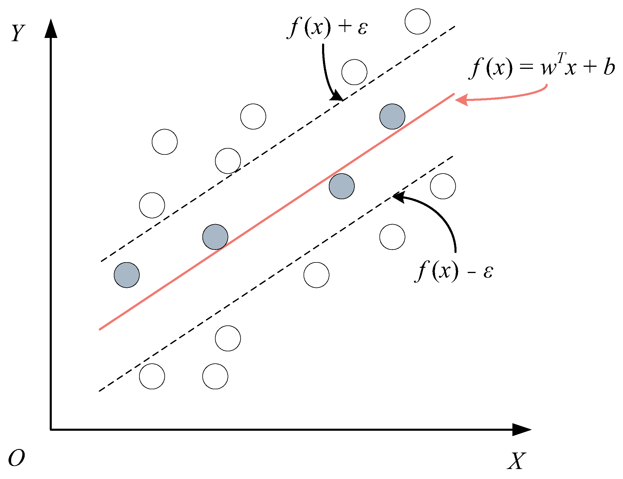
Support Vector Regression (SVR) is a nonparametric machine learning representative algorithm based on the kernel function, which has strong generalization ability. The computational objective is to find an optimal segregated hyperplane in the feature space and to use the minimization of structural risk to find the optimal regression hyperplane in the high-dimensional feature space. The basic principle is to map the low-dimensional feature space data to the high-dimensional feature space by introducing a kernel function [
30]. The formula for the SVR is as follows:
where
f(
x) represents the SVR model;
Φ(
x) represents the eigenvector after mapping
x and
w and
b are model parameters. In this study, the kernel function used is the Gaussian kernel, which can be expressed as follows:
where
κ represents the Gaussian kernel and
σ Represents the bandwidth of the Gaussian kernel. The training of the SVR model can be regarded as optimizing the model parameters to minimize the structural risk function. Different from the traditional regression model, SVR assumes that there is a maximum deviation of
ε between
f(
x) and the target value
y—that is, only when the absolute value of the difference between
f(
x) and
y is greater than
ε—as shown in
Figure 3.
The formula can be formalized as follows:
where
C is the regularization constant,
lε is the insensitive loss function,
ε is the tolerable deviation of SVR between
f(
x) and target value
y and
lε can be expressed as the following:
The SVR model fits the known data well and predicts the unknown data accurately, so it is used to predict the complex aeroengine exhaust gas temperature nonlinear problem.
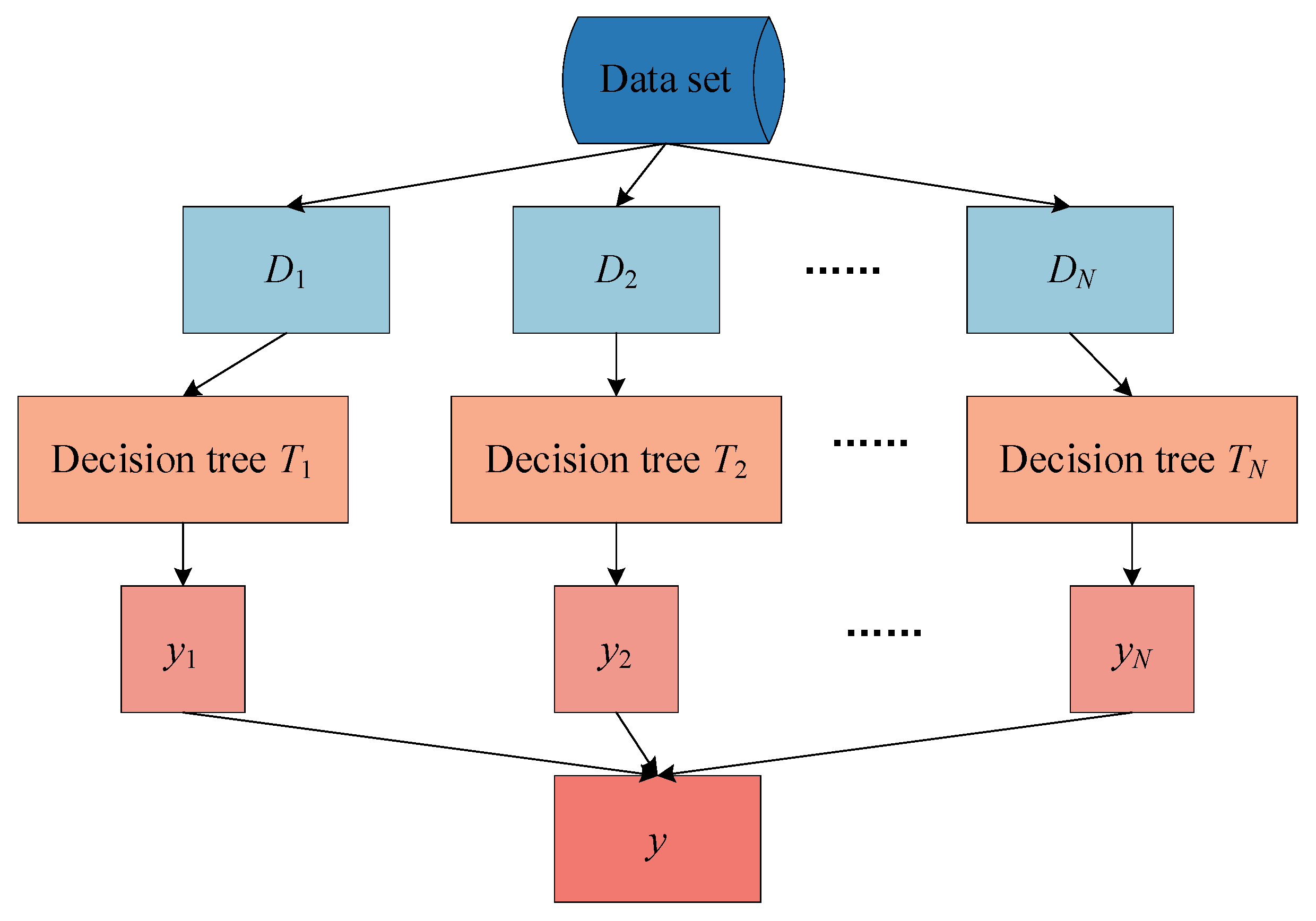
2.4. The RF
The RF is a supervised machine learning algorithm based on integrated learning. Integrated learning is a type of learning in which different types of algorithms are used or the same algorithms can be added multiple times to form stronger prediction models. The RF combines multiple algorithms of the same type, that is, trees for multiple decisions, so it is called ‘RF’. The decision tree is the building block of the RF, which is composed of many decision trees. Just as forests are collections of trees, the RF model predicts the final result by averaging the predicted results for each decision tree and is also considered collections of decision tree models. Each tree in the RF trains a subset of data, making the RF a powerful modeling technology that is much more powerful than a single decision tree. For regression problems, the final output is the average of all decision tree outputs. The basic idea behind the RF is to combine multiple decision trees to determine the final output, rather than relying on individual decision trees. When all decision trees are grouped in parallel, the error results are low because each decision tree is perfectly trained for a particular sample data [
31].
The process of the RF is shown in
Figure 4. In this study, the RF works as follows:
Randomly select N subsets of samples from the dataset.
Build a decision tree based on these N sample subsets.
Select the number of trees you want in the algorithm and repeat steps 1 and 2.
Each tree in the forest predicts the y value (output) and calculates the final value by averaging the predicted values of all decision trees in the forest.
Since the RF is insensitive to noise in the training set and uses an unrelated set of decision trees more robustly than a single set, which can avoid fitting problems, the RF algorithm has attracted much attention in the field of machine learning. This paper also chooses the RF as one of the models to build the exhaust gas temperature baseline of the aeroengine.
3. Prediction Process Framework
3.1. Data Preprocessing
The dataset for the EGT baseline model were derived from the ACARS (Aircraft Ratio Addressing and Reporting System) message data provided by an airline company. The aircraft health management and status monitoring based on the ACARS data can improve the fleet engineering management capability and maintenance efficiency and reduce the occurrence of aircraft abnormal events; the ACARS data has been widely used in various fields of civil aviation. However, as a complex thermodynamic system, the aeroengine has a complex working state and measurement noise of on-board sensors. These factors may lead to the additional influence of input parameters in the original aeroengine ACARS message data on model results, so the original data must be preprocessed.
3.1.1. Data Filtering
Airborne sensors are inevitably disturbed by various factors when recording data, which leads to abnormal data containing noise values. Therefore, noise reduction of the original aeroengine message data is needed. The Kalman Filter (KF) has been widely used in engine sensor data noise reduction due to its robustness [
32]. In this paper, the Unscented Kalman Filter (UKF) is used for data denoising. Assuming the measurement noise is Gaussian white noise, the calculation process is
UT transformation near the estimated point, calculating the mean and variance of the point set, and then performing nonlinear mapping to obtain the state probability density function [
33]. The nonlinear system of UKF can be represented as follows:
where
f is the nonlinear state equation function,
H is the nonlinear observation equation function
W(
k) and
V(
k) is the Gaussian white noise of the covariance matrix.
3.1.2. Data Cleaning
Since the airborne sensors may have signal transmission failure, part of the original aeroengine ACARS message data may be lost, and machine learning algorithms generally cannot handle the characteristics of missing data, which will lead to data quality degradation. Therefore, the missing values in the message data must be cleared to improve the data quality. In this paper, we use the Exponentially Weighted Moving Average (EWMA) to complete the missing values from the existing values. The expression is as follows:
where EWMA(
t) represents the estimated value
t,
Y(
t) represents the actual measured value at
t,
n represents the total number of data and
a represents the weight coefficient of historical measured values. The traditional moving average method replaces the missing value by calculating the arithmetic mean of the data on both sides of the missing value, while EWMA uses the moving average weighted by exponential decline, and the weight of each value decreases exponentially over time. The closer the data are, the heavier the weight is and the farther the data are also given a certain weight [
34]. The working conditions and conditions of the engine will change constantly, so EWMA can better cope with these sudden changes.
3.1.3. Data Scaling
When the magnitude scale of the input parameters varies greatly, the machine learning algorithm may not perform well. It is usually solved by scaling the data to make them have the same magnitude scale. In this study, minimum–maximum normalization is used to scale the data so that the original value is mapped to the set range. The formula is as follows [
35]:
where
xmax and
xmin are the maximum and minimum values of the data, and
x*
max and
x*
min are the newly preset maximum and minimum values. In this study, the setting range of
x*
max and
x*
min is [0, 1].
3.1.4. Data Partitioning
In data division, aeroengine ACARS message data are divided into a training set and a test set. The training set is used to learn and adjust the internal parameters of the model, and the test set is used to evaluate the performance of the model after learning. Data partitioning can avoid unnecessary deviation of the learning results of the model and ensure the universality of the model after learning as much as possible. In this study, 2170 data samples were extracted, and all data samples were preprocessed. Among them, 2000 data samples formed a training set, and 170 data samples formed a training set. Theoretically, the results of the model in the training set and test set should be basically the same.
3.2. Establishment of the Baseline Model
The model of the engine in this paper is the CFM56-5B engine, which is a two-axis turbofan engine with the large bypass. There are five gas path rotating parts: fan, low-pressure compressor, high-pressure compressor, high-pressure turbine and low-pressure turbine. The aeroengine ACARS message data usually only include the deviation value between the measured
EGT and the
EGT provided by the original equipment manufacturer (OEM).
EGT baseline value is obtained from this, and its formula is the following:
where
EGTOEM represents the baseline value of
EGT,
EGTm represents the measured value of
EGT and Δ
EGTOEM indicates the
EGT deviation value provided by the OEM.
The engine parameters recorded in ACARS message data include engine oil volume,
EGT, total power, low-pressure speed (
N1), high-pressure speed (
N2), fuel flow (
Wf), flight altitude (
H), total atmospheric temperature (
TAT), flight Mach number (
Ma), etc. Engine
EGT is affected by many factors. According to the literature [
36,
37], the parameters related to
EGT extracted from ACARS data are listed in
Table 1, including
H,
TAT,
Ma,
N1,
N2 and
Wf. Since they are the main parameters that affect the change of
EGT, these factors were used as input parameters of the baseline model, and the
EGTOEM was used as the output target of the model. To clarify the impact of these factors on
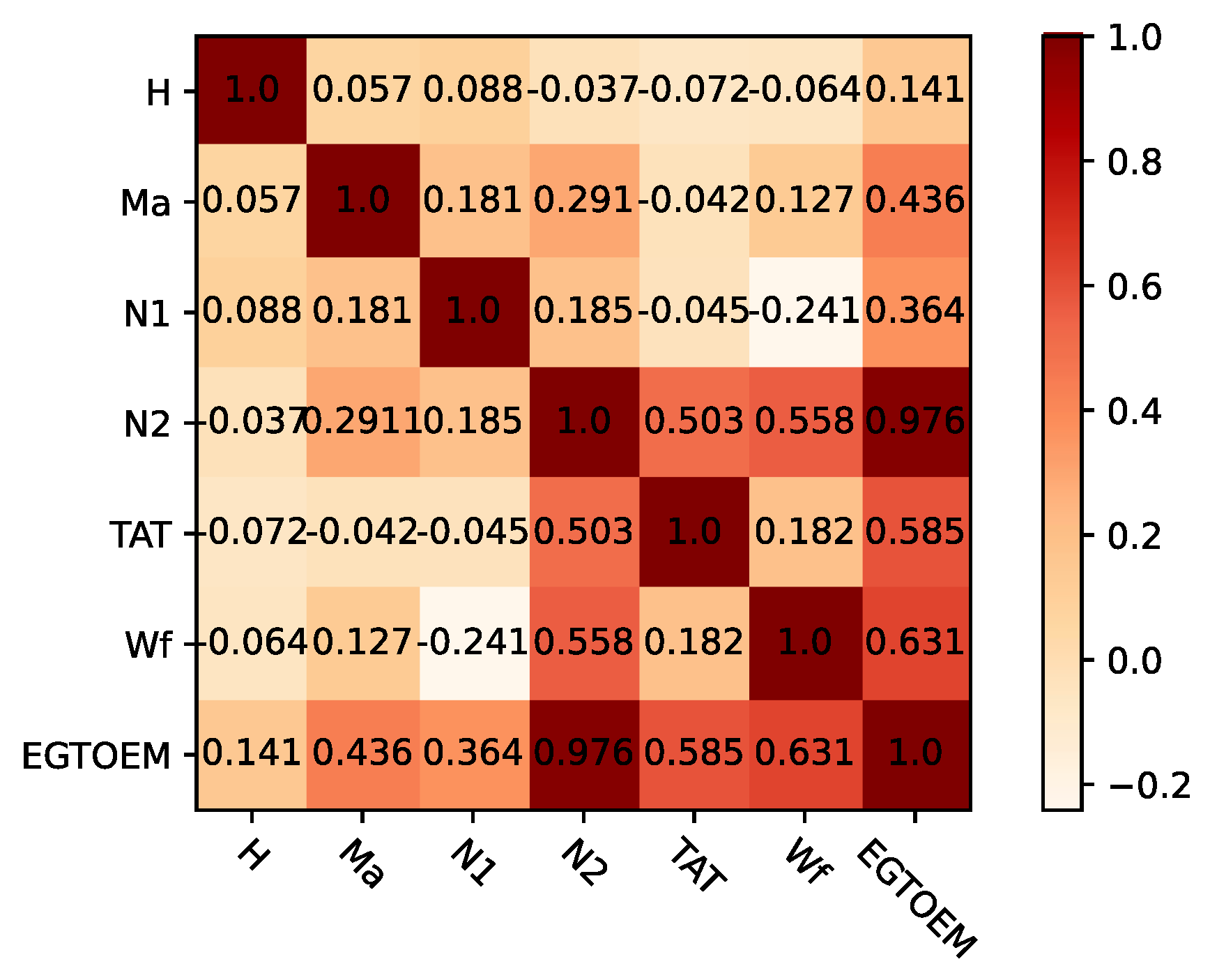
EGT baseline prediction, we conducted a correlation analysis on the training dataset according to Equations (16) and (17), as shown in
Figure 5.
where
cov(
X,
Y) is covariance calculation function;
X and
Y means the data of different features and
n is the sample number.
σX is the standard deviation of
X, and
σY is the standard deviation of
Y.
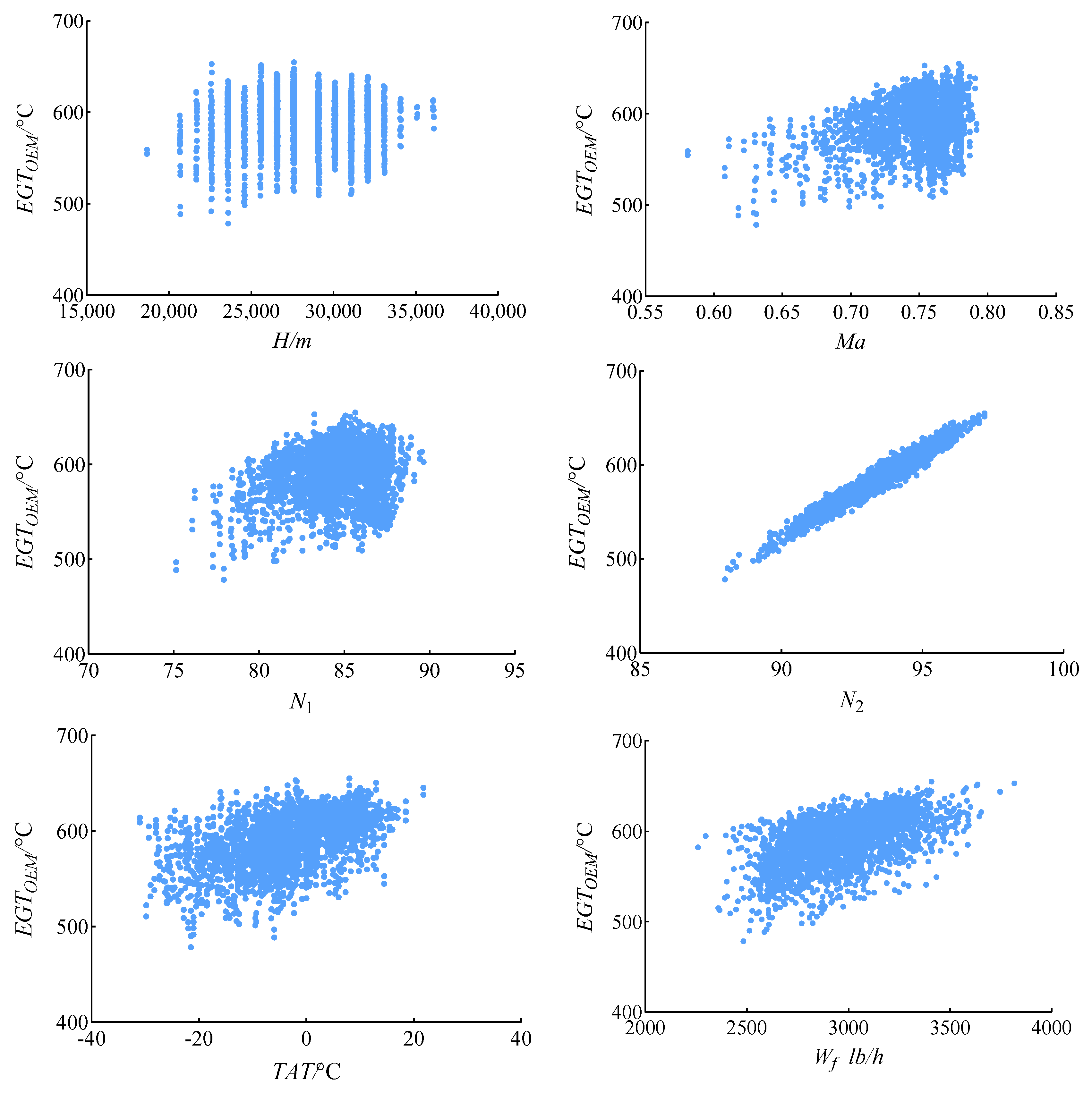
Figure 6 shows the scatter plot of these six parameter variables relative to
EGTOEM; the rotational speed is dimensionless. It can be seen that these parameters are highly correlated with
EGTOEM, so these parameters are considered to predict
EGTOEM. In addition, it can be seen that most parameters are positively correlated with
EGTOEM, and
N2 is significantly positively correlated with
EGTOEM. Compared with other parameters, the distribution of
H is not uniform because the flight altitude recorded by ACARS data in cruise state is relatively stable.
Ma is mainly distributed in the high-speed area, which is positively correlated with
EGTOEM.
TAT and
Wf are more widely distributed, and their effects on
EGTOEM are obviously positively correlated.
The
EGT baseline model can be expressed as follows:
In the formula, function f is used to characterize the nonlinear function between EGTOEM and the parameters that cause the change of EGT
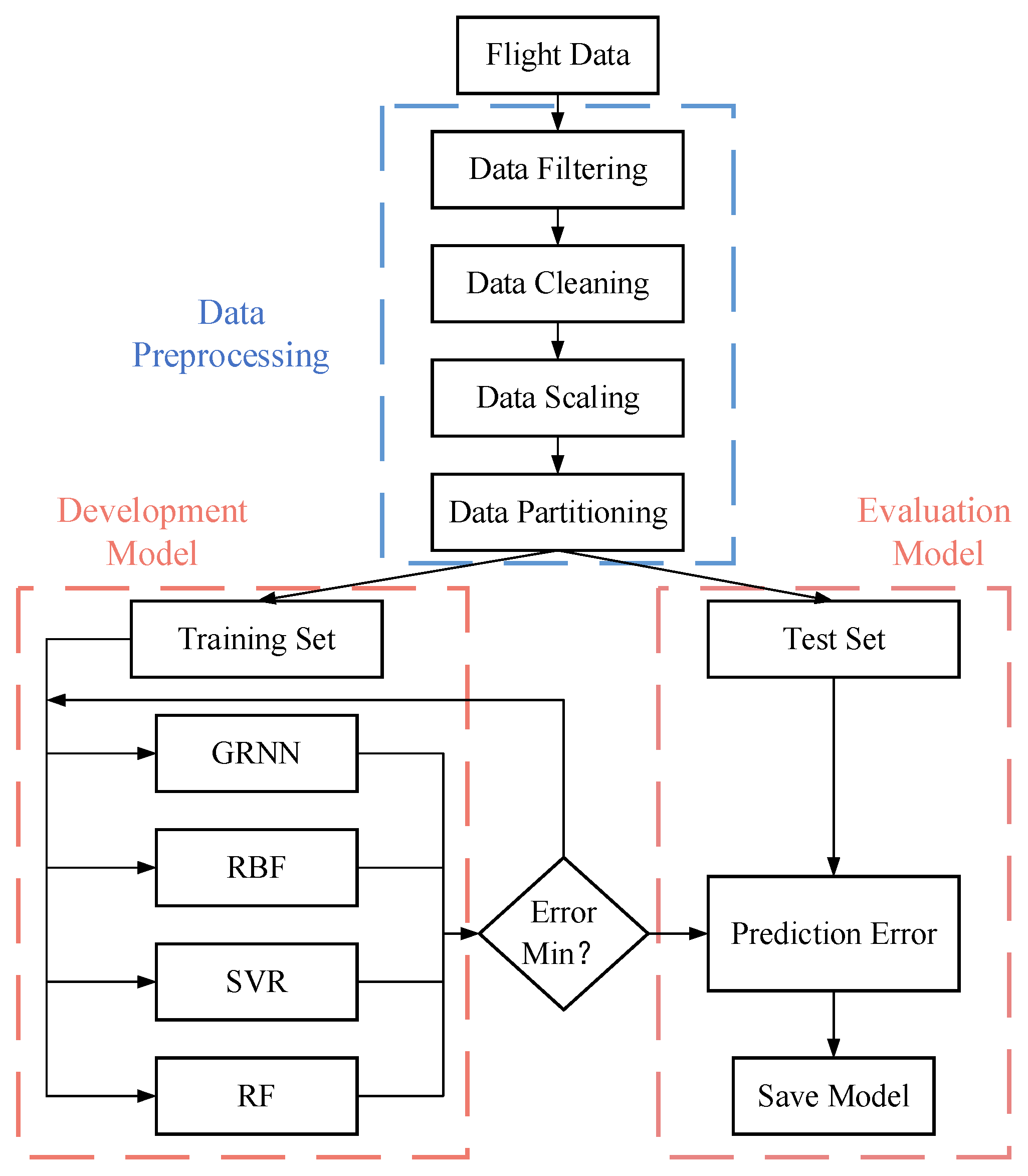
3.3. Process Framework
The process framework of
EGT baseline modeling is shown in
Figure 7, which mainly includes four steps:
Step 1: Obtain the aeroengine ACARS message data. The data in this paper come from the ACARS cruise message data of the CFM56-5B engine provided by an airline.
Step 2: Preprocessing of the original data. According to the engine type and gas path performance analysis method studied, the required input parameters are extracted; UKF is used for data noise reduction, and EWMA is used to complete missing data from existing data. The minimum–maximum normalization is used to scale the data, and the data are divided into a training set and a test set.
Step 3: Model development training. In this study, the GRNN, RBF, SVR and RF are used as basic machine learning methods, and EGT baseline model was developed using the training set.
Step 4: Test and evaluate the model. In this link, the data of the test set will be input into the trained model, and the performance of the model will be evaluated by the error between the predicted value calculated by the model and the actual value of the test set.
4. Case Study
The aeroengine message data in this study come from the ACARS cruise message data of the CFM56-5B engine provided by an airline in 2021, which is based on the health status or the post flight data of new engines. In this study, 2170 data samples of an aeroengine were extracted, and all data samples were preprocessed. Among them, 2000 data samples formed a training set, and 170 data samples formed a training set. Each raw data sample includes engine operating condition parameters (H, Ma), operating state parameters (N1, N2, Wf) and total engine exhaust temperature (EGT).
4.1. Training Result Analysis
In the training process, all the super parameters within the model will be continuously optimized until the training error of the model reaches the minimum to determine the optimal network structure. The four machine learning methods were developed under the language environment of MATLAB2020, and their settings are as follows:
GRNN. The GRNN follows the deep learning architecture shown in
Figure 1. The epochs and the batch size are set to 50 and 100, respectively.
RBF. The RBF follows the deep learning architecture shown in
Figure 2. Among them, the learning rate
η is set to 0.3, the number of hidden layer nodes is set to 7 and epochs and the batch size are set to 50 and 100, respectively.
SVR. The regularization parameter C in the SVR is set to 1 × 10³, γ is set to 0.1, ε is set to 1 × 10⁻³.
RF. The maximum depth, number of estimators and random state of the RF are set to 30, 100 and 2, respectively.
At the same time, the above methods are run on a PC with the AMD Ryzen 9 3900X CPU and Kingston 3200 MHz 32G memory in subsequent calculations to prevent other factors from having an additional impact on the performance evaluation of the model.
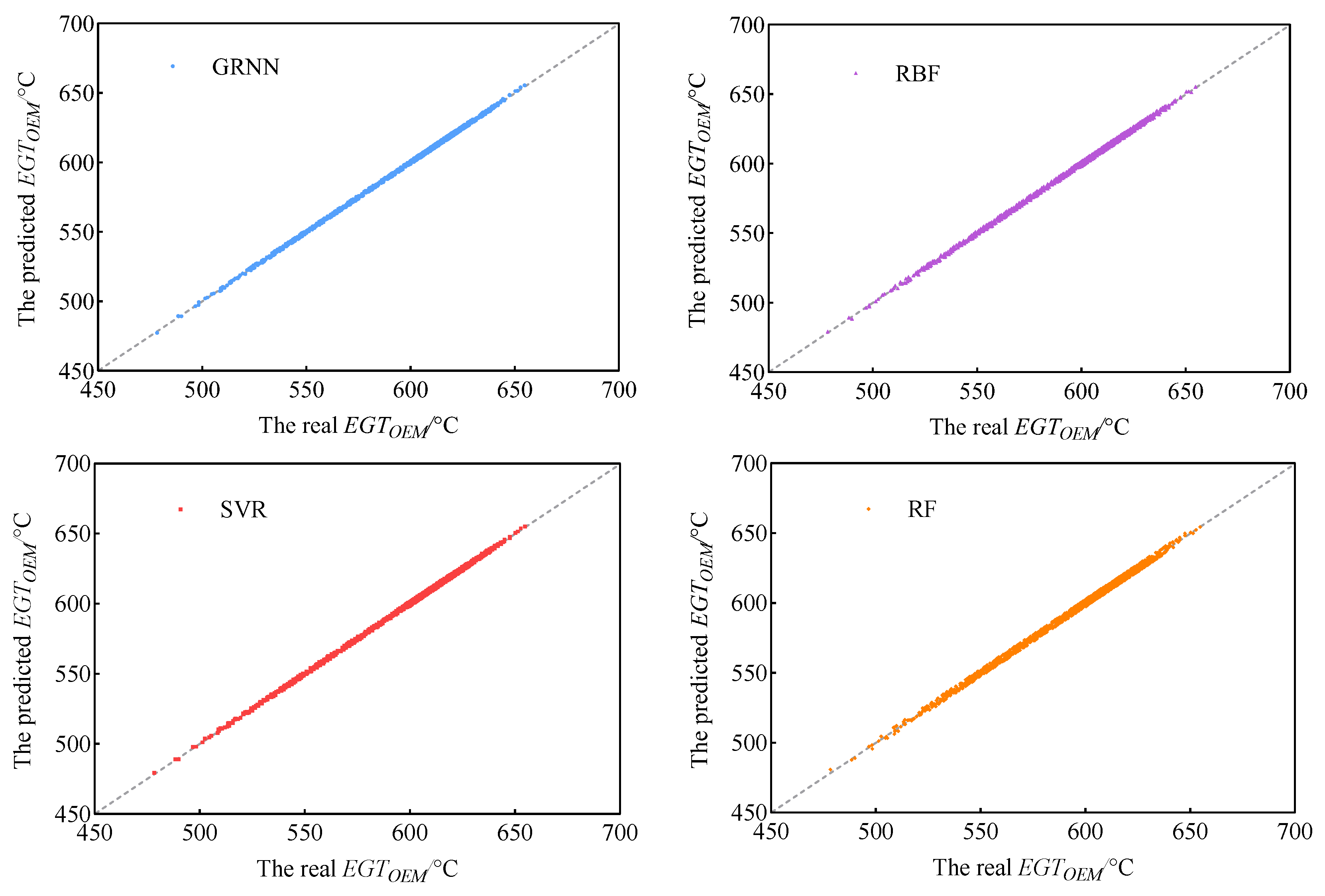
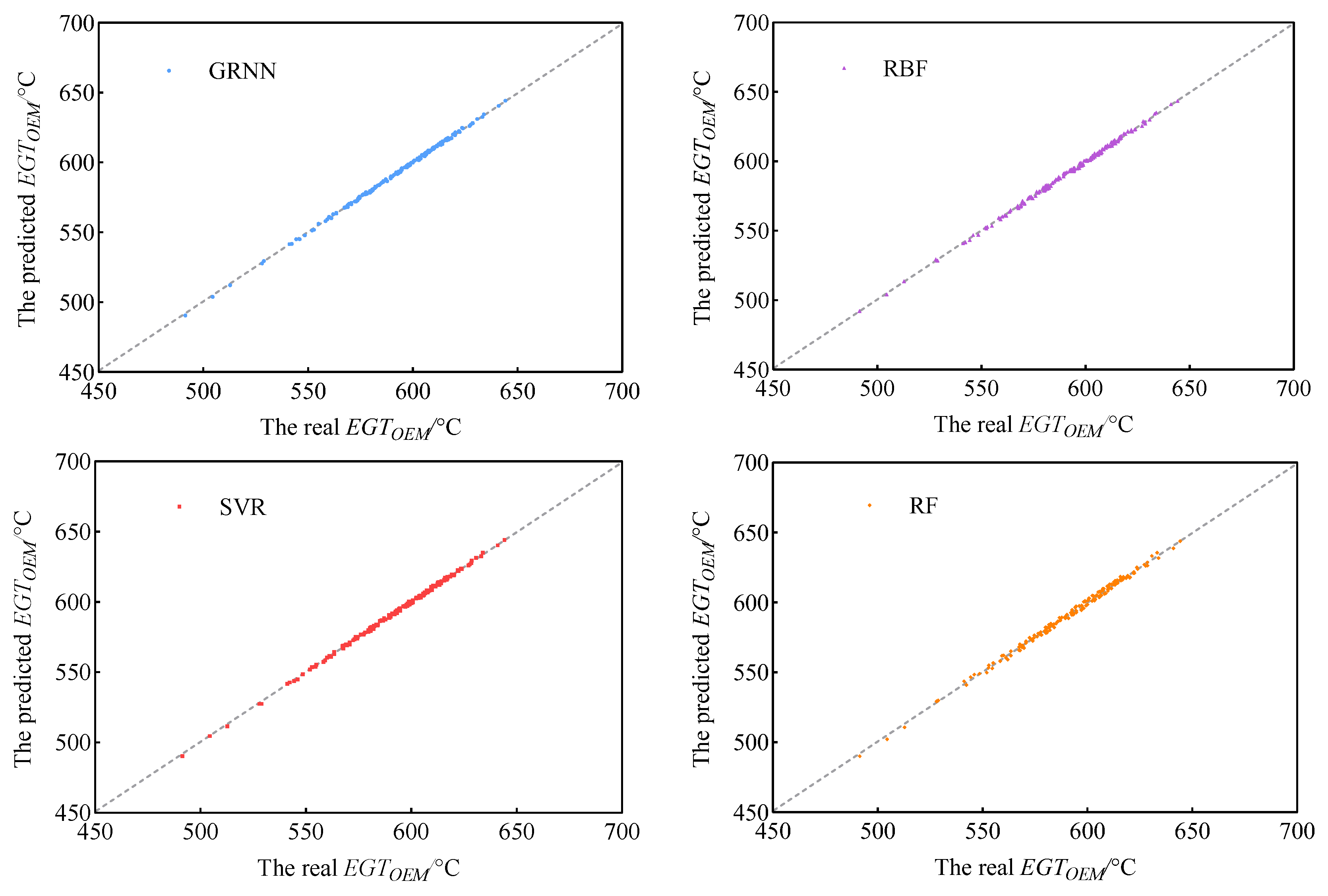
Figure 8 shows the training results of four machine learning models. From the detailed comparison in the figures, it can be seen that the training results of each model are basically consistent with the actual situation, and in most cases, their prediction points are almost at the accurate location of the 45° diagonal straight line in the figure. Prediction points from the GRNN and SVR are almost perfectly aligned with the 45°diagonal line, making it difficult to distinguish them. The prediction accuracy of the RF is slightly lower than other models. In order to better evaluate the training accuracy of these machine learning methods, this paper introduces the following equation comparison indicators, which are widely used to describe the prediction accuracy of data.
Relative error (RE) is calculated as follows:
where
yi and
y*i represent the actual value and predicted value of the
i-th data sample, respectively.
Mean absolute error (MAE) is calculated as follows:
Root mean square error (RMSE) is calculated as follows:
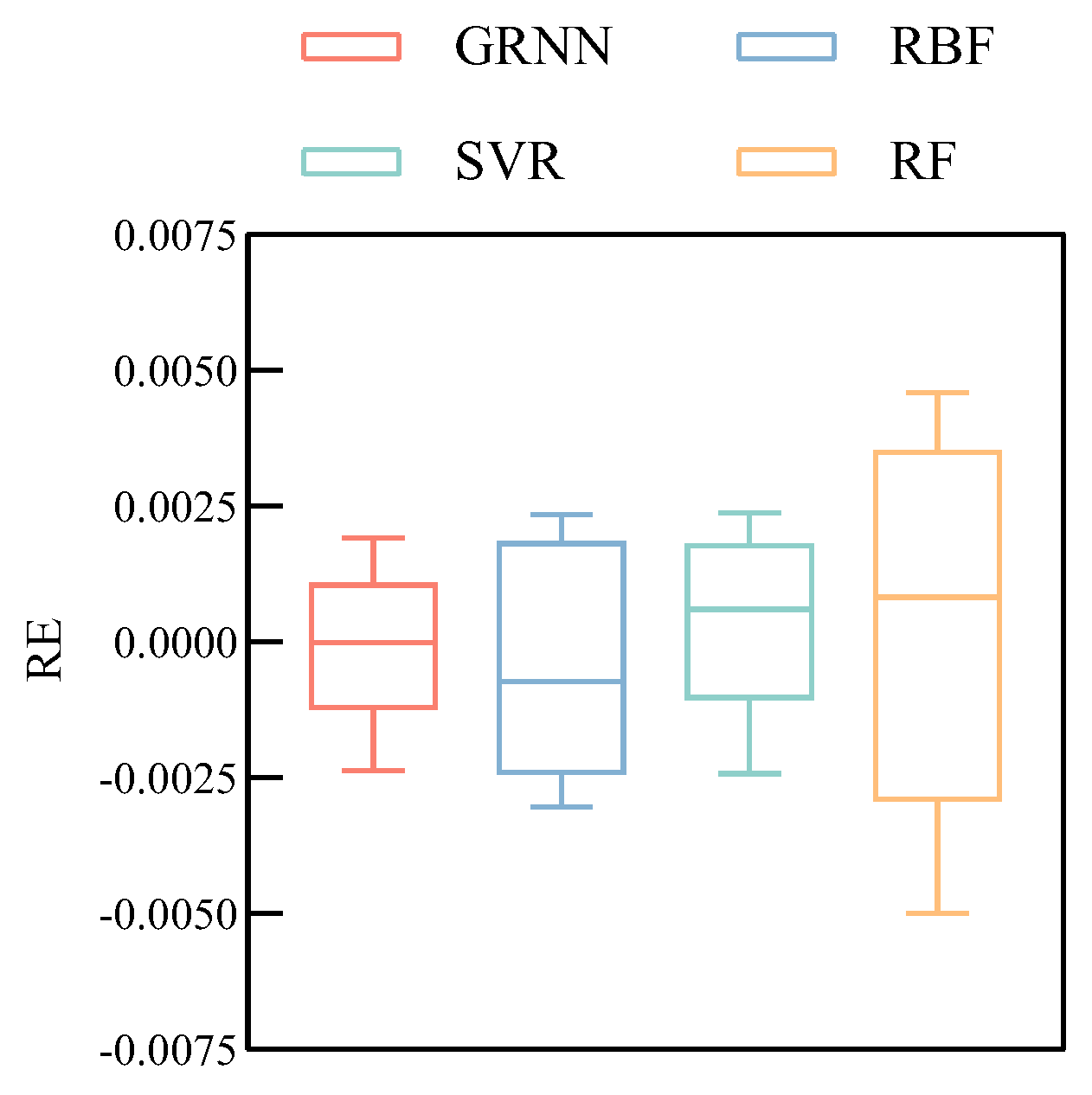
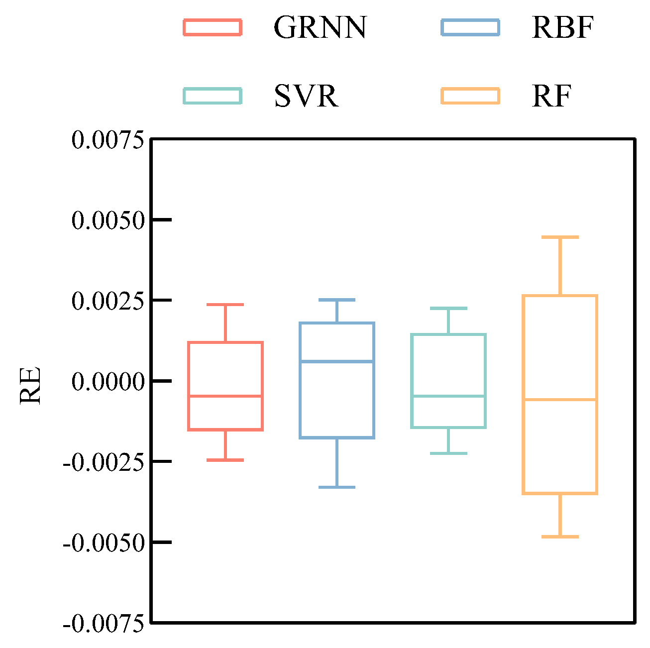
Figure 9 shows the training relative error block plot of each machine learning algorithm to further compare the training accuracy of each algorithm used.
Figure 7 shows that the GRNN and SVR have similar and lower relative errors of the training results, which means that the GRNN and SVR have better error accuracy. In contrast, the relative errors of training results from the RBF and RF are more widely dispersed in the figure, which indicates that their performance in predicting engine
EGT baseline is inferior to the GRNN and SVR.
Table 2 lists the MAE and RMSE of the training results of the four machine learning algorithms.
The RE results in
Figure 9 are similar to the predictions in
Table 2 and
Figure 8. The RE of the RBF and RF is widely distributed between ±0.15% and ±0.23%, while the RE of the GRNN and SVR can be well limited between ±0.10% and is significantly smaller than the RE of the RBF and RF. At the same time, it can be seen from
Table 2 that the training results of all models are very accurate. The MAE and RSME of the RBF are 1.496 × 10
−3 and 1.015, the MAE and RSME of the SVR are 1.141 × 10
−3 and 0.765, the MAE and RSME of the RF are 2.261 × 10
−3 and 1.435, the MAE and RSME of the GRNN are the lowest and their MAE and RSME are 1.092 × 10
−3 and 0.739, which indicates that the relative accuracy of the GRNN training results can reach 99.89% (calculated in (100%-MAPE)). At the same time, under the same calculation conditions, 2000 data points are processed, and the GRNN costs 4.43 × 10
−2 s in CPU time, the RBF costs 5.25 × 10
−2 s in CPU time, the RF costs 7.14 × 10
−2 s in CPU time, the SVR costs 4.92 × 10
−2 s in CPU time. The computing time of the GRNN is the lowest, indicating the highest computing efficiency. Although the training accuracy of these four algorithms is different, the actual deviation between them is very small. The lowest RF model training result accuracy can still reach 99.74%, which is enough to meet practical engineering applications.
4.2. Test Result Analysis
To further evaluate the prediction stability of the four machine learning algorithms,
Figure 10 and
Figure 11 and
Table 3 show the comparison of the prediction performance of the four algorithms in 170 sets of sample data test sets.
Figure 10 shows the test results of four machine learning models. It can be seen from
Figure 10 that the prediction points from the GRNN, RBF and SVR are almost at the exact position of the 45° diagonal line in the figure, and it is difficult to distinguish them. The prediction points of the RF have slight deviations from the 45° diagonal line in the figure. It can be seen that the GRNN, RBF and SVR have better prediction performances because their prediction points coincide more perfectly with the 45° diagonal line in the figure. There are slight deviations between the prediction points of the RF and the 45° diagonal in the figure, which means that its prediction performance is inferior to that of the GRNN, RBF and SVR.
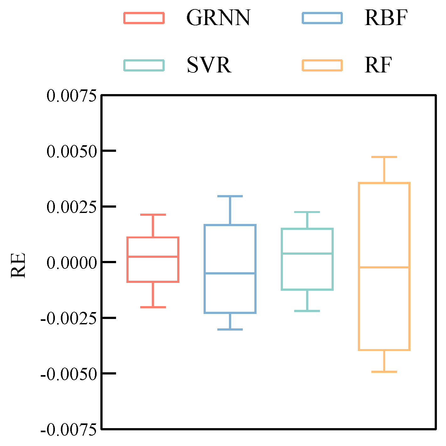
The prediction results in
Figure 11 are similar to those in
Table 3 and
Figure 10. The RE of the RBF and RF are widely distributed between ±0.16% and ±0.25%, while the RE of the GRNN and SVR can be well limited between ±0.12%, which is significantly smaller than the RE of the RBF and RF.
Table 3 shows the performance comparison of prediction results using 170 data sample points. In the table, the GRNN performs best in the engine
EGT baseline prediction, and its corresponding MAE and RSME are 1.094 × 10
−3 and 0.746, respectively, which indicates that the relative accuracy of the test results of the GRNN can also reach 99.89%. The MAE and RSME of the RBF are 1.513 × 10
−3 and 1.019, respectively, and the MAE and RSME of the RF are 2.276 × 10
−3 and 1.496, respectively. The prediction performance of the SVR is close to that of the GRNN, and its corresponding MAE and RSME are 1.126 × 10
−3 and 0.772, respectively. At the same time, under the same calculation conditions, when 170 data points are processed, the RBF costs 5.547 × 10
−3 s in CPU time, the RF costs 6.029 × 10
−3 s in CPU time, the SVR costs 1.9776 × 10
−3 s in CPU time, while the GRNN only costs 1.193 × 10
−3 s in CPU time, and the calculation time of the GRNN is the lowest, so the calculation efficiency is the highest. All the prediction error results of the four algorithms are consistent with the previous training set, and the differences between these algorithms are actually very small. Even if the RF can also achieve 99.77% of the test accuracy, all methods can achieve at least 99% of the prediction accuracy, which shows that these methods can be well used for engine
EGT baseline prediction.
4.3. Instance Verification
In order to further verify and compare the generalization ability and applicability of several algorithm models constructed in this paper, the ACARS flight data of another engine of the same model are selected as the verification sample, and the number of samples extracted after data processing is 500.
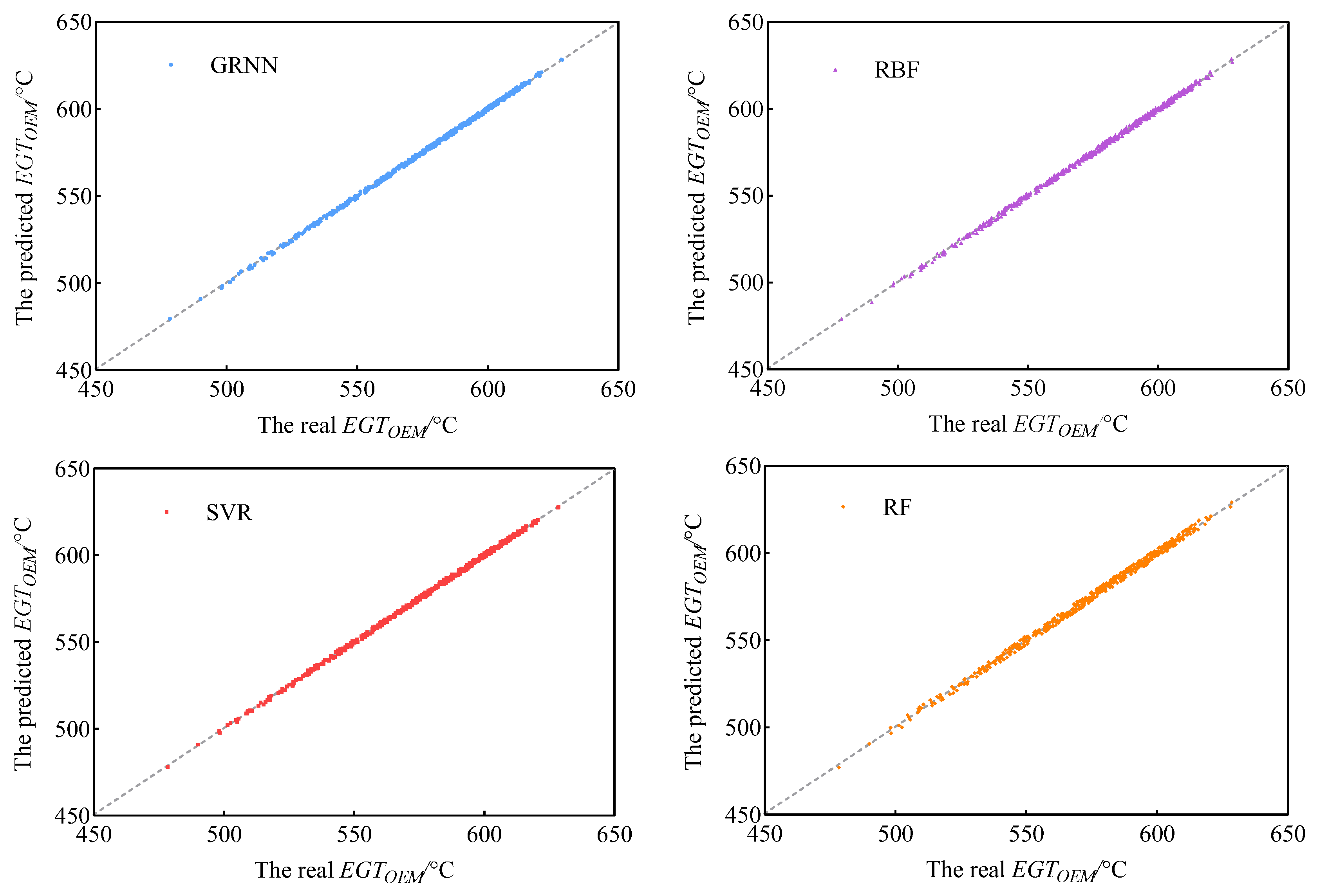
Figure 12 shows the verification results of four machine learning models. As shown in
Figure 12, almost all prediction points from the GRNN, RBF and SVR are precisely located at the exact position of the 45° diagonal line in the figure, while the prediction points from the RF are slightly different from the 45° diagonal line in the figure, which means that its prediction performance is inferior to that of the GRNN, RBF and SVR. It can be further seen from
Figure 11 what the RE differences of the four methods are. The convergence range of the GRNN and SVR is ±0.125%, while the RE of RBF and RF varies greatly between ±0.2% and ±0.25%, which is very consistent with the results in
Figure 11, indicating that the GRNN has better error accuracy.
Table 4 shows the performance comparison of the validation results using 500 data sample points. The results in
Table 4 are consistent with those in
Figure 12 and
Figure 13. The GRNN performs best in the engine
EGT baseline prediction, and its corresponding MAE and RSME are 1.132 × 10
−3 and 0.768, the MAE and RSME of the RBF are 1.538 × 10
−3 and 1.032, respectively; the MAE and RSME of the RF are 2.312 × 10
−3 and 1.507, respectively. The prediction performance of the SVR is close to that of the GRNN, and its corresponding MAE and RSME are 1.179 × 10
−3 and 0.781, respectively. All validation results of the four algorithms are consistent with those of the previous training set and test set, and the relative accuracy of the GRNN model validation results can still reach 99.88%. At the same time, under the same calculation conditions, 500 data points are processed, and the GRNN costs 3.512 × 10
−3 s in CPU time, the RBF costs 16.284 × 10
−3 s in CPU time, the RF costs 17.743 × 10
−3 s in CPU time, the SVR costs 5.812 × 10
−3 s in CPU time. The computing time of the GRNN is the lowest, indicating the highest computing efficiency. From the example verification, it can be seen that the GRNN is superior to the other models in predicting the engine
EGT baseline, with the highest calculation efficiency and higher prediction accuracy. The difference between these algorithms is actually very small. Even the RF can achieve 99.76% verification accuracy, and all methods can achieve at least 99% prediction accuracy, which shows that these methods can be well used for engine
EGT baseline prediction.
By comparing the calculation results in
Section 4.1 and
Section 4.2, four typical machine learning methods can achieve very good consistency for three different data samples. The GRNN and the SVR have better prediction accuracy, especially in the case study of testing and verification, and the GRNN uses the least CPU time to process the dataset and has the highest calculation efficiency. The GRNN is different from the output layer of the RBF in that it uses nonparametric estimation for subsequent probability processing, which has stronger advantages in nonlinear mapping ability and learning speed. The GRNN is an optimal regression, which can converge to more sample aggregation locations, is insensitive to sample data size, and is better at handling unstable data. The SVR has high classification accuracy and strong generalization ability when the sample size is not mass data, but it has no general criteria for selecting kernel functions for nonlinear problems and is sensitive to missing data, which may be the reason why its accuracy is slightly lower than the GRNN. Although the RF can better avoid over fitting, more trees lead to slower computing speed, so the RF consumed more computing time than other methods. All case studies show that the GRNN has better prediction accuracy, while the RBF can be ranked third. The difference between the four methods is very small, and the prediction accuracy of all four algorithms is very high, above 99%, which is applicable to the prediction of the engine
EGT baseline. In addition, the four typical machine learning methods for prediction purposes can also be used to predict other engine state parameter baselines in theory.
5. Conclusions
In this paper, CFM56-5B engine ACARS flight data were taken as a dataset, four data-driven frameworks were developed to predict engine EGT baseline, the relationship between EGT and other parameters were established. H, AT, Ma, N1, N2 and Wf were taken as input variables, and EGTOEM were taken as output variables in the prediction frameworks. Four different machine learning models were used to establish prediction frameworks, including the GRNN, RBF, SVR and RF. The prediction performance of four methods were compared and evaluated, and the main conclusions are as follows:
- (1)
The accuracy of all machine learning models can be higher than 99%, which meets the requirements of airlines. In particular, the GRNN used the same data to obtain lower errors than other machine learning models. In the training, testing and verification of EGT baseline model, the MAE of the GRNN are 1.092 × 10⁻³, 1.094 × 10⁻³ and 1.132 × 10⁻³, respectively.
- (2)
By comparing the calculation time of each model, it can be found that the GRNN has the best calculation efficiency. In the training, testing and verification of EGT baseline model, the GRNN consumed in CPU computing time 4.43 × 10⁻² s, 1.193 × 10⁻³ s and 3.512 × 10⁻³ s, respectively.
The methodologies can be employed by airlines to predict EGT baseline for the purpose of engine performance monitoring and health management and help airlines save maintenance costs. The EGT baseline models developed in this study have high accuracy and calculation efficiency. The prediction frameworks can effectively provide EGT baseline data, together with historical operating data, to quantify engine performance degradation.


