Low-Energy Transfer Design of Heliocentric Formation Using Lunar Swingby on the Example of LISA

Abstract

Space-based gravitational wave (GW) detection at low frequencies is of great scientific significance and has received extensive attention in recent years. This work designs and optimizes the low-energy transfer of the heliocentric formation of GW detectors, which starts from a geosynchronous transfer orbit and targets an Earth-like orbit. Based on the example of the Laser Interferometer Space Antenna (LISA), the transfer is first designed in two-body dynamical models and then refined in simplified high-fidelity dynamical models that only consider the major orbital perturbations evaluated here. The main contributions of this work are to present an adaptive model continuation technique and to exploit the lunar swingby technique to reduce the problem-solving difficulty and velocity increment of orbital transfer, respectively. The adaptive model continuation technique fully reveals the effect of perturbations and rapidly iterates the solutions to the simplified models. The simulation results show that the lunar swingby does reduce the energy needed to escape the Earth’s sphere of influence. It is found that the gravitation of the Earth–Moon system has a significant contribution to reducing the velocity increment. The solution of low-energy transfer in the simplified models is that the duration is 360.6615 days and the total velocity increment is 0.8468 km/s.

1. Introduction

Albert Einstein predicted the existence of gravitational waves (GW) based on general relativity, starting the research and discussion on gravitational-wave astronomy. The orbital-period decay measurements of binary pulsar PSR 1913+16 are consistent with the gravity theory of general relativity, indirectly suggesting the existence of GW [1,2]. However, the most convincing evidence for the existence of GW should be their direct detection, which is much more difficult. After decades of efforts, the Laser Interferometer Gravitational-Wave Observatory (LIGO) observed a transient GW signal named GW150914 in 2015, demonstrating the existence of binary stellar-mass black hole systems, which is the first direct detection of GW in human history [3]. The signal GW170817 [4], observed in 2017 by the Advanced LIGO and Advanced Virgo gravitational-wave detectors, is the first from binary neutron star inspiral. The signal GW200105 [5], observed in 2020 by LIGO–Virgo detector network, is the first from two compact binary coalescences. Henceforward a new observational window in physics has been opened.

GWs are unique and intensely informative about astrophysical processes, supporting the exploration of some of the most pressing problems in fundamental physics, astrophysics, and cosmology. The current detection approaches include ground-based detectors, space-based detectors, pulsar timing arrays, cosmic microwave background polarization, etc. Of the observatories mentioned above, those ground-based detectors detect the high-frequency part of the GW spectrum from ∼10 Hz to ∼10 kHz. The sensitivity of the ground-based detector is limited by the seismic noise, thermal noise, dynamic gravity gradient noise, quantum noise, and anthropogenic noise. Therefore, the relatively pure and low-frequency GWs are expected to be observed by space-based detectors [6,7]. LISA is an ESA-led space-based detector collaborating with NASA with well-proven technology. It was proposed by the LISA Consortium (an international collaboration of scientists) to observe GWs in the frequency range from $\sim {10}^{-4}$ Hz to $\sim {10}^{-1}$ Hz in the last century and was selected as a cornerstone mission in the ESA Horizon 2000-plus program [8]. LISA Pathfinder (LPF) is a dedicated technology validation mission for space-based detectors [9] operating from 2016 to 2017. LPF measured the essential performance and operation related to the stability, such as the drag-free and attitude control system [10] and noise performance [11], and validated the technical maturity of the LISA mission [12].

ESA made a proposal on the detailed concepts of the LISA mission and planned a launch around 2030 [13]. In this proposal, LISA is an equilateral triangle constellation separated by $2.5\times {10}^9$ m in Earth-trailing or Earth-leading heliocentric orbits at an angular distance of around 20 degrees. Existing orbital studies on LISA mainly concentrated on the formation design [14,15,16,17], but fewer on the orbital transfer. In the original LISA mission, the total velocity increment of three main transfer maneuvers in 16 months of transfer duration is estimated between 1.5∼2.1 km/s [18]. Bastante et al. proposed a transfer strategy of five impulses for adjusting the inclination, eccentricity, and phase angle to give a solution guess for solving the low-thrust transfer optimization problem through a gradient restoration algorithm [19]. Sweetser analyzed the end-to-end impulsive transfer process of a constellation of three spacecraft launched together into a heliocentric orbit trailing the Earth’s orbit by 20 degrees [20]. Xia et al. analyzed the relationship between the total velocity increment and the flight time and the relationship between the total velocity increment and the trailing angle behind the Earth by solving the Lambert’s problem. They further designed the transfer orbits, including the launch stage and the separation stage [21]. Joffre et al. studied the transfer design from the Earth towards Earth-Displaced Heliocentric Orbits in the Sun–Mean Earth–Moon Barycentre rotating frame [22]. The seasonal variations of the required velocity increment with the direct transfer strategy were calculated and analyzed, and then other alternative transfer strategies were suggested to reduce the fuel consumption and improve the compatibility of the launch. Martens et al. considered the relationship between the transfer velocity increment and the location of the constellation and optimized them together. They designed the transfer orbit using solar electric propulsion and analyzed the effect of insertion errors in the navigation process on the constellation stability [23].

The above studies involve the design of LISA’s transfer orbits. It is obvious that the optimal transfer design of heliocentric formation reduces the fuel requirement for the GW observation mission. To achieve this purpose, a practical approach is to fully consider and exploit the effects of multi-body dynamics [24,25]. However, among the existing studies on the transfer design of the GW detectors, most are based on the two-body dynamical model, but few consider multi-body effects. On the one hand, the transfer design results in the two-body model have not yet been improved in any high-fidelity model [20,21]. For the transfer orbit of the GW detectors, the effect of the multi-body dynamics is significant [26,27], and the error of the orbit propogation under the two-body model should be relatively large. The transfer design under the Sun–Earth three-body model is more accurate than that under the heliocentric two-body model, but other complex perturbations still need to be considered [22]. This work further explores the effects of other perturbations on the transfer. The orders of magnitude of multiple perturbations are calculated, and those which significantly impact the orbit are identified. The adaptive model continuation technique is proposed in this paper to obtain quantitatively the influence of each perturbation on the velocity increment of the transfer. On the other hand, most existing studies have only completed the design of heliocentric transfer orbits, assuming that the starting of the transfer is on the Earth escape orbit [19,20,23]. However, the transfer within the Earth’s sphere of influence (SOI) should be elaborately designed to reduce the overall launch and transfer costs [28], especially to increase the energy to escape the Earth’s SOI by the lunar swingby [29,30,31]. It is well known that the geosynchronous transfer orbit (GTO) is always used as an intermediate orbit for spacecraft with the destinations of high-altitude orbits such as geosynchronous or geostationary orbits. Thus, rather than directly launching the spacecraft into an Earth escape orbit, this work starts the transfer design from a GTO that can be reached by Ariane 5 [32] and, of course, is still within the Earth’s SOI. We are devoted to working out a well-designed low-energy transfer that positively exploits the perturbations in the Earth’s SOI to reduce the total velocity increment of transfer. Based on the above considerations, this work studies the design of low-energy impulsive transfer from a GTO to the center of the heliocentric formation in simplified high-fidelity dynamical models by utilizing the lunar swingby technique and the adaptive model continuation technique.

The remainder of this paper is organized as follows. In Section 2, the optimization problem and the dynamics are introduced. In Section 3, the approach for low-energy transfer design is described in detail. Specific design results for each stage are given in Section 4. Finally, conclusions are drawn in Section 5.

2. Problem Description

In this section, the optimization problem is described, and the reference frames and equations of motion for orbital transfer are presented.

2.1. Optimization Problem Statement

The start of the transfer is set to a GTO. The initial state of the spacecraft (S/C) is described by the classical orbital elements (COE), of which the values of semi-major axis (a), eccentricity (e), inclination (i), and argument of perigee ($\omega$) are fixed, and the right ascension of ascending node ($\Omega$) and the true anomaly (f) are considered as optimization variables. The end of the transfer is determined as an Earth-Tailing Heliocentric Orbit with 20 degrees behind the Earth [13], which is the center of the constellation, and the angle between the plane of the constellation and the ecliptic is 60 degrees, as shown in Figure 1. The high-thrust chemical thrust is applied to perform the orbital maneuvers, and the maneuvering process is considered as instantaneous impulses. Assume that the impulse vector is denoted by $\Delta \mathit{v}$, and the time moments immediately before and after the impulse are denoted by $t^{-}$ and $t^{+}$, respectively. The position and velocity vectors satisfy the following relations:

$$\left\{\begin{array}{c}\mathit{r}\left(t^{+}\right)=\mathit{r}\left(t^{-}\right)\hfill \\ \mathit{v}\left(t^{+}\right)=\mathit{v}\left(t^{-}\right)+\Delta \mathit{v}\hfill \end{array}\right.$$

(1)

For the general multi-impulse transfer problem, the process can be described as follows: the S/C maneuvers from a GTO into the transfer orbit at the beginning and reaches the terminal orbit at the end after several impulses. The transfer design problem in this work can be constructed as a nonlinear optimization problem. The optimization variables include the time moments and impulse vectors of several maneuvers. The problem needs to meet the boundary conditions as follows:

$$\left\{\begin{array}{c}a\left(t_s\right)=a_{\mathrm{GTO}},e\left(t_s\right)=e_{\mathrm{GTO}},i\left(t_s\right)=i_{\mathrm{GTO}},\omega \left(t_s\right)={\omega }_{\mathrm{GTO}}\hfill \\ a\left(t_f\right)=a_{\mathrm{E}},e\left(t_f\right)=e_{\mathrm{E}},i\left(t_f\right)=i_{\mathrm{E}},\Omega \left(t_f\right)={\Omega }_{\mathrm{E}},\omega \left(t_f\right)={\omega }_{\mathrm{E}},f\left(t_f\right)=f_{\mathrm{E}}-{20}^{\circ }\hfill \end{array}\right.$$

(2)

where $t_s$ and $t_f$ represent the initial and terminal time moments, respectively. The subscripts, GTO and E, represent the COE of the GTO and the Earth, respectively. The time constraint needs to be satisfied:

$$t_f-t_s<T_{max}$$

(3)

Other engineering constraints are not considered in this work. In practical problems, if requirements for communication, measurement, control, etc., need to be satisfied, their constraints should be added to the optimization problem. The objective is to minimize the total velocity increment:

$$minJ=\Delta V=\sum _{i=1}^n\parallel \Delta {\mathit{v}}_i\parallel$$

(4)

where n denotes the total number of impulses, and $\parallel ·\parallel$ represents the 2-norm.

2.2. Reference Frames

In this work, the following frames are used to describe the motion of the S/C.

• J2000 Earth-centered inertial (ECI) frame: The origin is at the center of the Earth. The basic plane ($XY$ plane) is the mean equator of epoch J2000.0, and the X-axis points to the intersection of the mean equator of J2000.0 with the mean ecliptic plane.
• J2000 Moon-centered inertial (MCI) frame: The origin is at the center of the Moon, and the directions of the three axes are the same as the J2000 ECI frame.
• Heliocentric equatorial reference frame (HERF): The origin is at the center of the Sun, and the directions of the three axes are the same as the J2000 ECI frame.

Let us denote the position and velocity vectors by $\mathit{r}$ and $\mathit{v}$, respectively. The superscript (E) denotes the position and velocity vectors with respect to the Earth in the J2000 ECI frame, the superscript (M) denotes the pair with respect to the Moon in the J2000 MCI frame, and the superscript (S) denotes the pair with respect to the Sun in the HERF. The subscripts represent the pair of the spacecraft, the Moon, and the Earth, respectively. The following relationships exist when describing the motion of spacecraft in different frames.

$$\left\{\begin{array}{c}{\mathit{r}}_{\mathrm{S}/\mathrm{C}}^{\left(\mathrm{E}\right)}={\mathit{r}}_{\mathrm{S}/\mathrm{C}}^{\left(\mathrm{M}\right)}+{\mathit{r}}_{\mathrm{Moon}}^{\left(\mathrm{E}\right)},{\mathit{v}}_{\mathrm{S}/\mathrm{C}}^{\left(\mathrm{E}\right)}={\mathit{v}}_{\mathrm{S}/\mathrm{C}}^{\left(\mathrm{M}\right)}+{\mathit{v}}_{\mathrm{Moon}}^{\left(\mathrm{E}\right)}\hfill \\ {\mathit{r}}_{\mathrm{S}/\mathrm{C}}^{\left(\mathrm{S}\right)}={\mathit{r}}_{\mathrm{S}/\mathrm{C}}^{\left(\mathrm{E}\right)}+{\mathit{r}}_{\mathrm{Earth}}^{\left(\mathrm{S}\right)},{\mathit{v}}_{\mathrm{S}/\mathrm{C}}^{\left(\mathrm{S}\right)}={\mathit{v}}_{\mathrm{S}/\mathrm{C}}^{\left(\mathrm{E}\right)}+{\mathit{v}}_{\mathrm{Earth}}^{\left(\mathrm{S}\right)}\hfill \end{array}\right.$$

(5)

When calculating the motion of spacecraft for orbital transfer, the following frames are also involved:

• The second realization of the International Celestial Reference Frame (ICRF2) [33]: The origin is the solar system barycenter, with the basic plane ($XY$ plane) close to the mean equator of epoch J2000.0 and the X-axis close to the intersection of the mean equator of J2000.0 with the mean ecliptic plane. The planetary and lunar ephemerides such as Jet Propulsion Laboratory (JPL)’s DE430 and DE431 [34] are described in this frame.
• Earth Centered Earth Fixed (ECEF) frame: The origin is at the center of the Earth. The X-axis is at the intersection of the Greenwich Meridian and the equatorial plane. The Z-axis is collinear with the Earth’s spin axis and points to the north.

The ICRF2 is an improved version of the first realization of the International Celestial Reference Frame (ICRF1) [35]. The ICRF1 is approximately consistent with the FK5 pole of J2000.0, and there are differences between the mean J2000.0 pole and the ICRF1 pole of ≈19 mas in ecliptic longitude and ≈4 mas in obliquity, which are within the error of the stellar realization. Therefore, the differences in the directions of the axes between the ICRF2 and HERF are not considered in this work.

Define the following rotation matrices:

$${\mathit{R}}_x\left(\alpha \right)=\left[\begin{array}{ccc}1& 0& 0\\ 0& cos\alpha & -sin\alpha \\ 0& sin\alpha & cos\alpha \end{array}\right],{\mathit{R}}_y\left(\alpha \right)=\left[\begin{array}{ccc}cos\alpha & 0& sin\alpha \\ 0& 1& 0\\ -sin\alpha & 0& cos\alpha \end{array}\right],{\mathit{R}}_z\left(\alpha \right)=\left[\begin{array}{ccc}cos\alpha & -sin\alpha & 0\\ sin\alpha & cos\alpha & 0\\ 0& 0& 1\end{array}\right]$$

(6)

Suppose ${\left(\underline{\mathit{r}}\right)}_{\mathrm{ECEF}}$ and ${\left(\underline{\mathit{r}}\right)}_{\mathrm{ECI}}$ denote the column arrays of the same vector in the J2000 ECI frame and ECEF frame, respectively, and the transition relationship between them is [36,37]:

$${\left(\underline{\mathit{r}}\right)}_{\mathrm{ECEF}}={\mathit{R}}_{EE}{\mathit{R}}_{ET}{\mathit{R}}_{TM}{\mathit{R}}_{MJ}{\left(\underline{\mathit{r}}\right)}_{\mathrm{ECI}}$$

(7)

The expressions for these matrices are as follows:

$$\left\{\begin{array}{c}{\mathit{R}}_{EE}={\mathit{R}}_y\left(x_p\right){\mathit{R}}_x\left(y_p\right)\hfill \\ {\mathit{R}}_{ET}={\mathit{R}}_z\left(-{\theta }_{GST}\right)\hfill \\ {\mathit{R}}_{TM}={\mathit{R}}_x(\overline{\epsilon }+\Delta \epsilon ){\mathit{R}}_z(\Delta \psi ){\mathit{R}}_x(-\overline{\epsilon })\hfill \\ {\mathit{R}}_{MJ}={\mathit{R}}_E\left(z_A\right){\mathit{R}}_y\left(-{\theta }_A\right){\mathit{R}}_z\left({\zeta }_A\right)\hfill \end{array}\right.$$

(8)

where $x_p$ and $y_p$ denote the components of polar motion, ${\theta }_{GST}$ denotes the Greenwich sidereal time, ${\zeta }_A$, $z_A$, and ${\theta }_A$ denote the precession of the equinoxes, $\overline{\epsilon }$ denotes the mean obliquity, and $\Delta \psi$ and $\Delta \epsilon$ denote the nutations in longitude and in obliquity, respectively [38]. The polar motion is set to zero due to its unpredictability many years later. Note that the transformation between the ECI and ECEF frames, expressed by Equations (7) and (8), will be used in the high-fidelity dynamical model for the geocentric orbits that considers perturbations, including especially the Earth’s nonspherical gravitation. This work will design and optimize the low-energy transfer in a simplified high-fidelity dynamical model for the geocentric orbits that regards the Earth as a rotating ellipsoid with regular angular velocity and will then investigate the solution error between the simplified high-fidelity model and the high-fidelity model, which will prove to be very small.

2.3. Equations of Motion for Orbital Transfer

The motion of the S/C can be divided into different phases according to the planetary SOI, and different central bodies are chosen to establish the equations of motion. According to the Earth’s SOI, the transfer orbit of S/C is composed of geocentric orbits and heliocentric orbits. As described in the following, the lunar swingby technique is adopted in order to increase the escape energy and reduce the required velocity increment of the transfer. Therefore, the selenocentric orbits are also included in the transfer. The transfer process of the spacecraft is shown in Figure 2. The 1st and 3rd segments belong to geocentric orbits, the 2nd segment belongs to selenocentric orbits, and the 4th segment belongs to heliocentric orbits.

In this work, there are three kinds of dynamical models for calculating the geocentric and heliocentric orbits: the two-body dynamical model, the simplified high-fidelity dynamical model, and the high-fidelity dynamical model, as shown in

Table 1. Different dynamical models of the geocentric orbits.

Perturbation	Two-Body Dynamical Model	Simplified High-Fidelity Dynamical Model	High-Fidelity Dynamical Model
Lunar gravitation	×	√	√
Nonspherical gravitation	×	√	√
Atmospheric drag	×	√	√
Solar gravitation	×	√	√
Solar radiation	×	√	√
Relativistic effects	×	×	√
Solid tides	×	×	√
Ocean tides	×	×	√
Rotation deformation	×	×	√

and

Table 2. Different dynamical models of the heliocentric orbits.

Perturbation	Two-Body Dynamical Model	Simplified High-Fidelity Dynamical Model	High-Fidelity Dynamical Model
Mercury gravitation	×	√	√
Venus gravitation	×	√	√
Earth gravitation	×	√	√
Mars gravitation	×	×	√
Jupiter gravitation	×	√	√
Saturn gravitation	×	×	√
Uranus gravitation	×	×	√
Neptune gravitation	×	×	√
Pluto gravitation	×	×	√
Lunar gravitation	×	√	√
Solar radiation	×	√	√

. There are two dynamical models for calculating the selenocentric orbits: the two-body dynamical model and the simplified high-fidelity dynamical model, as shown in

Table 3. Different dynamical models of the selenocentric orbits.

Perturbation	Two-Body Dynamical Model	Simplified High-Fidelity Dynamical Model
Earth gravitation	×	√
Solar gravitation	×	√
Solar radiation	×	√

. In Table 1, Table 2 and Table 3, the symbol × means that the perturbation is not considered, and the symbol √ means that the perturbation is considered. The transfer design will be first completed in the two-body models corresponding to the geocentric and heliocentric orbits, where the lunar swingby is equated to an instantaneous impulse. The segments of transfer orbit obtained in the two-body models will be used to calculate the perturbation accelerations counted into the high-fidelity models. We will simplify the high-fidelity models according to the orders of magnitude of the perturbation accelerations and the errors in the terminal state. Then, the transfer will be refined and corrected in the simplified high-fidelity models. Finally, the terminal state errors and the computational times of the transfer orbit will be individually compared between the simplified high-fidelity and high-fidelity models to support this simplification. The equations of motion of the spacecraft moving in the simplified high-fidelity models are given in this section, and the equations for the rest of the perturbation accelerations counted into the high-fidelity models can be referred to [36].

2.3.1. Equations of Motion on Geocentric Orbits

In the J2000 ECI frame, the equations of motion of the S/C is given by:

$$\left\{\begin{array}{c}\dot{\mathit{r}}=\mathit{v}\hfill \\ \dot{\mathit{v}}={\mathit{a}}_C+{\mathit{a}}_N+{\mathit{a}}_D+{\mathit{a}}_T+{\mathit{a}}_R\hfill \end{array}\right.$$

(9)

where $\mathit{r}$ and $\mathit{v}$ denote the position and velocity vectors with respect to the Earth in the J2000 ECI frame, respectively, ${\mathit{a}}_C$ denotes the central gravitational acceleration of the Earth, and ${\mathit{a}}_N$, ${\mathit{a}}_D$, ${\mathit{a}}_T$, and ${\mathit{a}}_R$ denote the accelerations caused by the Earth’s nonspherical gravitation, atmospheric drag, the third-body gravitation due to the Sun and Moon, and the solar radiation, respectively. The specific expressions of the perturbation accelerations are given below.

Since the Earth is not a regular sphere, the Earth’s nonspherical gravitation should be considered in addition to the central celestial body gravitation. In the ECEF frame, the potential function U of the Earth’s non-spherical gravitation is expressed in the form of a spherical harmonic function [39]:

$$U=\frac{{\mu }_{\mathrm{E}}}{r}\sum _{n=2}^{\infty }\sum _{m=0}^n{\left(\frac{R_{\mathrm{E}}}{r}\right)}^n{\overline{P}}_{nm}(sin\phi )\left({\overline{C}}_{nm}cosm\lambda +{\overline{S}}_{nm}sinm\lambda \right)$$

(10)

where $R_{\mathrm{E}}$ and ${\mu }_{\mathrm{E}}$ are the Earth’s reference radius and gravitational constant, respectively, $\phi$ and $\lambda$ are the geocentric latitude and geocentric longitude of the S/C in the ECEF frame, respectively, r is the geocentric distance, ${\overline{C}}_{nm}$ and ${\overline{S}}_{nm}$ are the normalized gravitational coefficients, and ${\overline{P}}_{nm}\left(u\right)$ is the normalized associated Legendre function of degree n and order m with respect to the variable u. In the simplified model for the geocentric orbits of this work, the Earth is simplified as a rotating ellipsoid, i.e., only ${\overline{C}}_{2,0}$ is considered, and note that $J_2=-{\overline{C}}_{2,0}=1.0826269\times {10}^{-3}$. Supposing the column array of $\mathit{r}$ in the J2000 ECI frame is ${[x,y,z]}^{\mathrm{T}}$, the column array of the Earth’s nonspherical gravitation acceleration (approximately equal to the $J_2$ perturbation acceleration) is:

$${\left(\underline{{\mathit{a}}_N}\right)}_{\mathrm{ECI}}\approx {\left(\underline{{\mathit{a}}_{J_2}}\right)}_{\mathrm{ECI}}=\frac{3}{2}\frac{{\mu }_{\mathrm{E}}{J}_2{R}_{\mathrm{E}}^2}{r^5}\left[\begin{array}{c}\frac{5x{z}^2}{r^2}-x\\ \frac{5y{z}^2}{r^2}-y\\ \frac{5z^3}{r^2}-3z\end{array}\right]$$

(11)

The acceleration of the atmospheric drag with area-mass ratio $S/m$ is:

$${\mathit{a}}_D=-\frac{1}{2}{C}_D\frac{S}{m}\rho \parallel \mathit{V}\parallel \mathit{V}$$

(12)

where $C_D$ is the atmospheric drag coefficient, $\rho$ the atmospheric density at the location of the S/C, and $\mathit{V}$ the velocity of the S/C relative to the atmosphere, calculated by the following equation:

$$\mathit{V}=\mathit{v}-{\mathit{\omega }}_{\mathrm{E}}\times \mathit{r}$$

(13)

where $\mathit{r}$ and $\mathit{v}$ are the position and velocity of the S/C with respect to the J2000 ECI frame, and ${\mathit{\omega }}_{\mathrm{E}}$ is the angular velocity vector of the Earth’s rotation. Supposing the column array of $\mathit{v}$ in the J2000 ECI frame is ${[v_x,v_y,v_z]}^{\mathrm{T}}$, the column array of $\mathit{V}$ in the J2000 ECI frame is approximated by:

$${\left(\underline{\mathit{V}}\right)}_{\mathrm{ECI}}=\left[\begin{array}{c}{v}_x+{\omega }_{\mathrm{E}}y\\ v_y-{\omega }_{\mathrm{E}}x\\ v_z\end{array}\right]$$

(14)

where ${\omega }_{\mathrm{E}}=\parallel {\mathit{\omega }}_{\mathrm{E}}\parallel$.

In addition to the Earth’s gravitation, the S/C is affected by the gravitation of the Sun, Moon, and other large planets. For the geocentric orbits in this work, only the gravitation of the Sun and Moon is considered. The perturbation acceleration of the third-body gravitation on the S/C is:

$${\mathit{a}}_T=-\sum _i{\mu }_i\left(\frac{\mathit{r}-{\mathit{r}}_i}{{∥\mathit{r}-{\mathit{r}}_i∥}^3}+\frac{{\mathit{r}}_i}{{∥{\mathit{r}}_i∥}^3}\right)$$

(15)

where ${\mu }_i=G{m}_i$ denotes the gravitational constant of the celestial body i, and ${\mathit{r}}_i$ denotes the position vector of the celestial body i with respect to the Earth in the J2000 ECI frame. Their column arrays of position vectors in the J2000 ECI frame are obtained directly from the planetary and lunar ephemerides.

In the J2000 ECI frame, the acceleration of the S/C from the solar radiation is expressed as:

$${\mathit{a}}_R=K{C}_R\frac{S}{m}\frac{L_s}{4\pi c}\frac{\mathit{r}-{\mathit{r}}_s}{{∥\mathit{r}-{\mathit{r}}_s∥}^3}$$

(16)

where $\mathit{r}$ and ${\mathit{r}}_s$ denote the position vectors of the S/C and the Sun with respect to the Earth in the J2000 ECI frame, respectively, $C_R$ the solar radiation coefficient, c the speed of light, $L_s$ the luminosity of the Sun, and K the visibility coefficient of the sunlight at the location of the S/C and is related to the ground-shadow model used. In this work, the simplification of $K\equiv 1$ is taken. The physical meanings of other symbols are the same as above.

2.3.2. Equations of Motion on Heliocentric Orbits

In the HERF, the equations of motion of the S/C is given by:

$$\left\{\begin{array}{c}\dot{\mathit{r}}=\mathit{v}\hfill \\ \dot{\mathit{v}}={\mathit{a}}_C+{\mathit{a}}_T+{\mathit{a}}_R\hfill \end{array}\right.$$

(17)

where $\mathit{r}$ and $\mathit{v}$ are the position and velocity with respect to the Sun in the HERF, respectively, ${\mathit{a}}_C$ the central gravitational acceleration of the Sun, ${\mathit{a}}_T$ the acceleration of the third-body gravitation due to the Earth–Moon system, Jupiter, Venus, and Mercury, and ${\mathit{a}}_R$ the acceleration of the solar radiation.

The acceleration of the third-body gravitation ${\mathit{a}}_T$ is calculated by Equation (15), where ${\mathit{r}}_i$ denotes the position vector of the celestial body i with respect to the Sun in the HERF, and ${\mu }_i=G{m}_i$ denotes the gravitational constant of celestial body i. Their column arrays of position vectors in the J2000 ECI frame are obtained directly from the planetary and lunar ephemerides. The acceleration of the solar radiation ${\mathit{a}}_R$ is expressed by Equation (16), where the vector difference $\mathit{r}-{\mathit{r}}_s$ should be replaced by $\mathit{r}$.

2.3.3. Equations of Motion on Selenocentric Orbits

In the J2000 MCI frame, the equations of motion of the S/C is given by:

$$\left\{\begin{array}{c}\dot{\mathit{r}}=\mathit{v}\hfill \\ \dot{\mathit{v}}={\mathit{a}}_C+{\mathit{a}}_T+{\mathit{a}}_R\hfill \end{array}\right.$$

(18)

where $\mathit{r}$ and $\mathit{v}$ are the position and velocity with respect to the Moon in the J2000 MCI frame, respectively, ${\mathit{a}}_C$ the central gravitational acceleration of the Moon, ${\mathit{a}}_T$ the acceleration of the third-body gravitation due to the Earth and Sun, and ${\mathit{a}}_R$ the acceleration of the solar radiation.

The acceleration of the third-body gravitation ${\mathit{a}}_T$ is calculated by Equation (15), where ${\mathit{r}}_i$ denotes the position vector of the celestial body i with respect to the Moon in the J2000 MCI frame, and ${\mu }_i=G{m}_i$ denotes the gravitational constant of the celestial body i. The acceleration of the solar radiation ${\mathit{a}}_R$ is calculated by Equation (16), where $\mathit{r}$ and ${\mathit{r}}_s$ here denote the position vectors of the S/C and the Sun with respect to the Moon in the J2000 MCI frame, respectively, and the physical meanings of other symbols are the same as above. Their column arrays of position vectors in the J2000 MCI frame are obtained directly from the planetary and lunar ephemerides.

3. Low-Energy Transfer Design

The transfer design of heliocentric formation in the high-fidelity models has challenges such as strong nonlinearity, sensitivity to initial values, and multiple locally optimal solutions. If the optimization problem is directly solved in the high-fidelity models, the computational burden is great, and the orbital perturbations may not be well utilized to reduce the velocity increment of the transfer. Therefore, the optimization is first carried out several times in the two-body models to quickly obtain multiple locally optimal solutions as candidates. Together with simplifying the dynamical models in Section 2, an adaptive model continuation technique will be proposed to iterate these multiple solutions from the two-body models to the simplified high-fidelity models, which will be completed quickly. Finally, the best solution among them is picked out as the design result. We compare the orbital terminal states and computational times under different dynamical models and verify that the simplification of the dynamical models is acceptable and effective.

In addition, the inclination of a GTO with respect to the Earth’s equator is $6^{\circ }$, and the angle between the equatorial plane and the ecliptic plane is about $23.{43}^{\circ }$. The inclination of the lunar orbit to the equatorial plane ranges from $18.{28}^{\circ }$ to $28.{58}^{\circ }$. It has potential to utilize lunar gravitation to reduce the transfer energy.

3.1. Design of Lunar Swingby

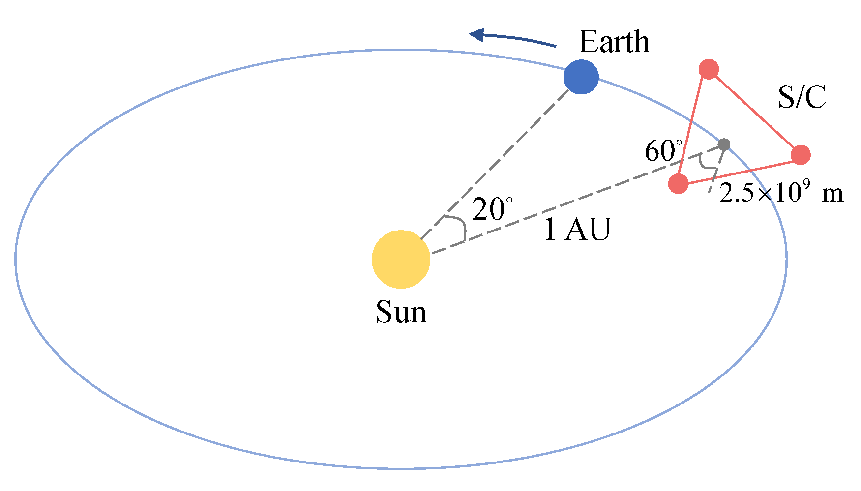
Limited to the launch vehicle capacity and the energy requirement for later science operation, the GW detection mission desires an ingenious transfer design with little transfer energy. Swingby is usually considered to reduce the velocity increment or transfer time. The orbit of the S/C is designed to pass near a planet and use its gravitation to increase the energy, change the inclination, reduce the mission time, and achieve other purposes. In this work, the lunar swingby is designed to reduce the velocity increment of transfer.

In the preliminary design, the swingby is modeled as an instantaneous impulse [40]. The differences in the positions and time moments immediately before and after the swingby are not considered, and the corresponding positions are consistent with the position of the swingby celestial body at the swingby time moment. In the lunar swingby, let us denote the time moments immediately before and after the swingby by $t_{-}$ and $t_{+}$, respectively, and the position vectors of the S/C with respect to the Earth in the J2000 ECI frame before and after the swingby by ${\mathit{r}}_{-}$ and ${\mathit{r}}_{+}$, respectively. The position vector of the Moon with respect to the Earth in the J2000 ECI frame at the time moment of the lunar swingby is denoted by ${\mathit{r}}_M$. The following relationships exist:

$$\left\{\begin{array}{c}{t}_{-}=t_{+}=t_M\hfill \\ {\mathit{r}}_{-}={\mathit{r}}_{+}={\mathit{r}}_M\hfill \end{array}\right.$$

(19)

The relative velocity between the S/C and the swingby celestial body is called hyperbolic excess speed and is denoted by ${\mathit{v}}_{\infty }$. Suppose that ${\mathit{v}}_{\infty }^{-}$ denotes the hyperbolic excess speed when entering the lunar SOI and ${\mathit{v}}_{\infty }^{+}$ denotes the hyperbolic excess speed when leaving the lunar SOI. They hold the forms:

$$\left\{\begin{array}{c}{\mathit{v}}_{\infty }^{-}={\mathit{v}}_{-}-{\mathit{v}}_M\hfill \\ {\mathit{v}}_{\infty }^{+}={\mathit{v}}_{+}-{\mathit{v}}_M\hfill \end{array}\right.$$

(20)

where ${\mathit{v}}_{-}$ and ${\mathit{v}}_{+}$ denote the velocity vectors of the S/C with respect to the Earth in the J2000 ECI frame immediately before and after the swingby, respectively, and ${\mathit{v}}_M$ denotes the position vector of the Moon with respect to the Earth in the J2000 ECI frame at the time moment of lunar swingby.

When the S/C is within the lunar SOI, only the lunar gravitation is considered, which means that the orbit of the S/C in the SOI is a hyperbolic curve. The turn angle of the hyperbolic curve, $\delta$, is determined by the swingby radius $r_M$, the magnitude of hyperbolic excess velocity $v_{\infty }$, and the gravitational constant of the Moon ${\mu }_M$:

$$\delta =2\arcsin \left(\frac{{\mu }_M}{{\mu }_M+r_M{v}_{\infty }^2}\right)$$

(21)

The hyperbolic excess speed ${\mathit{v}}_{\infty }^{+}$ lies on a circular cone with ${\mathit{v}}_{\infty }^{-}$ as the axis and $\delta$ as the top angle, and its magnitude is equal to ${\mathit{v}}_{\infty }^{-}$. The coordinate system $M-\xi \eta \zeta$ is established with the Moon as the center, as shown in Figure 3, where the $\xi$-axis is parallel to ${\mathit{v}}_{\infty }^{-}$, the $\zeta$-axis is parallel to the normal of the plane formed by ${\mathit{v}}_{\infty }^{-}$ and ${\mathit{v}}_M$, and the $\xi$-axis, $\eta$-axis and $\zeta$-axis form a right-handed coordinate system.

The unit vectors of the coordinate axes are denoted by $\mathit{i}$, $\mathit{j}$, and $\mathit{k}$:

$$\mathit{i}=\frac{{\mathit{v}}_{\infty }^{-}}{v_{\infty }},\mathit{k}=\frac{{\mathit{v}}_{\infty }^{-}\times {\mathit{v}}_M}{∥{\mathit{v}}_{\infty }^{-}\times {\mathit{v}}_M∥},\mathit{j}=\mathit{k}\times \mathit{i}$$

(22)

Assuming that no active orbital maneuver is applied during the swingby, the hyperbolic excess speed ${\mathit{v}}_{\infty }^{+}$ immediately after the lunar swingby and the velocity increment $\Delta v_{\mathrm{swingby}}$ obtained from the swingby are given by:

$$\begin{array}{c}\hfill {\mathit{v}}_{\infty }^{+}=v_{\infty }[cos\delta \mathit{i}+(sin\delta sin\psi )\mathit{j}+(sin\delta cos\psi )\mathit{k}]\end{array}$$

(23)

$$\begin{array}{cc}\hfill \Delta v_{\mathrm{swingby}}& ={\mathit{v}}_{\infty }^{+}-{\mathit{v}}_{\infty }^{-}={\mathit{v}}_{+}-{\mathit{v}}_{-}\hfill \\ \hfill & =v_{\infty }[(cos\delta -1)\mathit{i}+(sin\delta sin\psi )\mathit{j}+(sin\delta cos\psi )\mathit{k}]\hfill \end{array}$$

(24)

where $\psi$ denotes the angle between the projection of ${\mathit{v}}_{\infty }^{+}$ in the $\eta \zeta$ plane and the $\zeta$-axis, with values in the range $[0,2\pi )$. When ${\mathit{v}}_{\infty }^{-}$, $r_p$, and $\psi$ are determined, the velocity increment of the swingby, $\Delta v_{\mathrm{swingby}}$, and the hyperbolic excess speed after the swingby, ${\mathit{v}}_{\infty }^{+}$, can be obtained. In general, it is necessary to apply a maneuver after swingby to ensure reaching the next target.

The above impulsive model of swingby is an approximation, and it is suitable for the preliminary design of orbit. When the perturbations before swingby and the lunar SOI are considered, the initial state needs to be corrected if the effect of swingby in the initial design is to be achieved. In lunar and interplanetary trajectories, the B-plane coordinate system and B-plane parameters (notated as $BT$ and $BR$) are efficient in describing the arrival conditions at a target celestial body. The B-plane parameters are nearly linear functions of the initial orbital conditions [41].

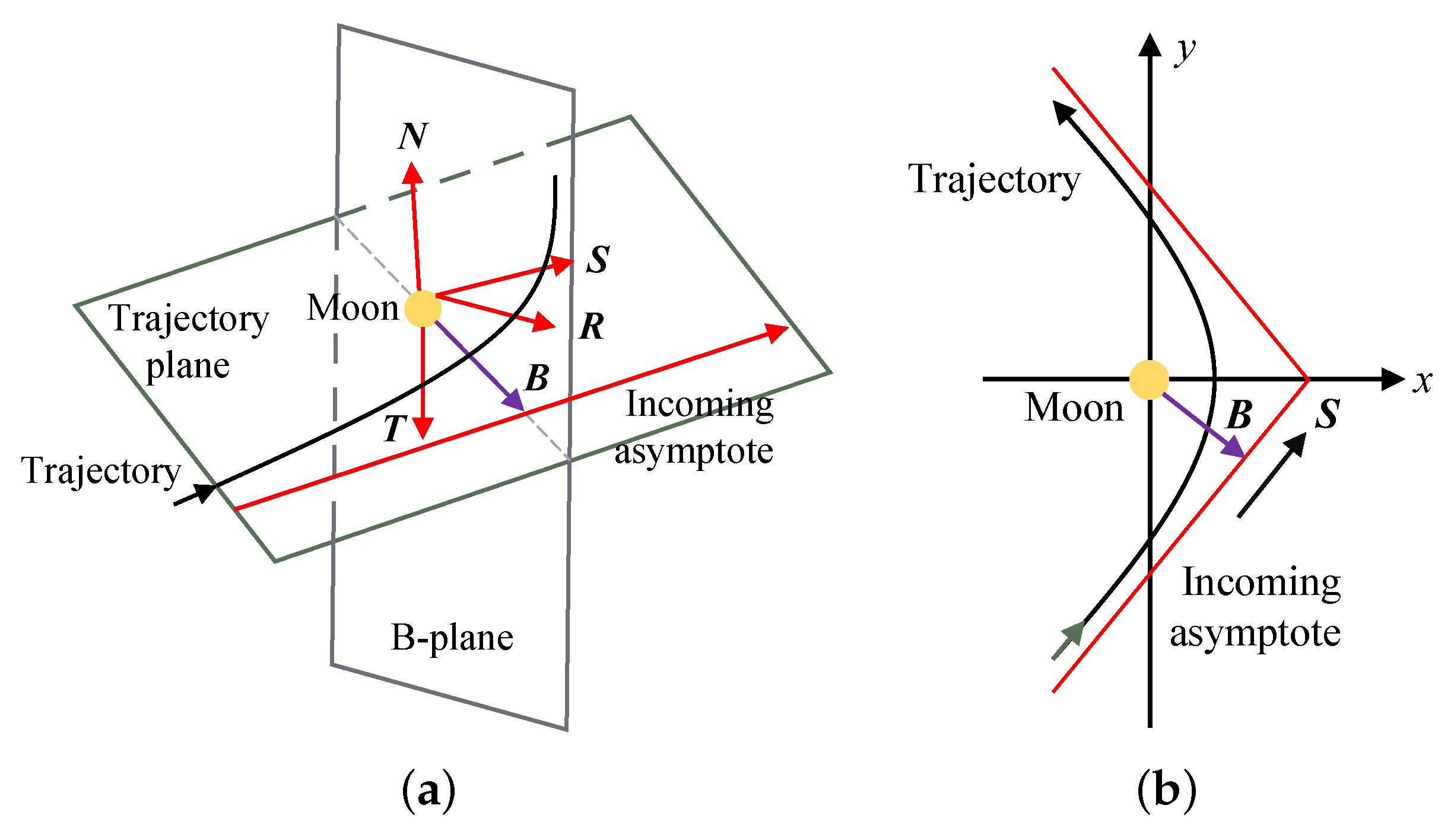
In the case of the lunar swingby, the B-plane is defined as the plane past the lunar center and perpendicular to the incoming asymptote of the S/C, and the vector $\mathit{B}$ points from the lunar center to the intersection of the B-plane and the incoming asymptote, as shown in Figure 4. The direction normal to the lunar orbit is adopted as the reference direction, denoted by $\mathit{N}$. The B-plane coordinate system is described by three orthogonal unit vectors $\mathit{S}$, $\mathit{R}$, and $\mathit{T}$, as shown in Figure 4. They are defined as:

$$\mathit{S}=\frac{{\mathit{v}}_{\infty }^{-}}{\parallel {\mathit{v}}_{\infty }^{-}\parallel },\mathit{T}=\frac{\mathit{S}\times \mathit{N}}{\parallel \mathit{S}\times \mathit{N}\parallel },\mathit{R}=\mathit{S}\times \mathit{T}$$

(25)

The B-plane parameters are the projections of $\mathit{B}$ on $\mathit{T}$ and $\mathit{R}$:

$$BT=\mathit{B}·\mathit{T},BR=\mathit{B}·\mathit{R}$$

(26)

The target B-plane parameters denoted by $B{T}_t$ and $B{R}_t$ are calculated from the hyperbolic excess speed ${\mathit{v}}_{\infty }^{-}$ and ${\mathit{v}}_{\infty }^{+}$ in the preliminary design, and the relationship between them satisfies Equations (20)–(24). The normal unit vector of the hyperbolic orbital plane is:

$${\mathit{n}}_t=\frac{{\mathit{v}}_{\infty }^{-}\times {\mathit{v}}_{\infty }^{+}}{\parallel {\mathit{v}}_{\infty }^{-}\times {\mathit{v}}_{\infty }^{+}\parallel }$$

(27)

The energy of the hyperbolic orbit, E, satisfies [42]:

$$E=\frac{1}{2}{∥{\mathit{v}}_{\infty }^{-}∥}^2-\frac{{\mu }_M}{∥{\mathit{r}}_{\infty }^{-}∥}=-\frac{{\mu }_M}{2a_t}$$

(28)

where ${\mathit{r}}_{\infty }^{-}$ denotes the position vector with respect to the Moon when entering the lunar SOI, and $a_t$ denotes the semi-major axis of the hyperbolic orbit. In fact, $\frac{{\mu }_{\mathrm{E}}}{∥{\mathit{r}}_{\infty }^{-}∥}$ is close to 0. Therefore, the semi-major axis $a_t$ of the hyperbolic orbit is approximated by the following equation:

$$a_t=-\frac{{\mu }_M}{{∥{\mathit{v}}_{\infty }^{-}∥}^2}$$

(29)

The magnitude of the vector ${\mathit{B}}_t$ is equal to the magnitude of the semi-imaginary axis of the hyperbolic orbit, $b_t$:

$$∥{\mathit{B}}_t∥=|b_t|=|a_t|cot\left(\frac{\delta }{2}\right)$$

(30)

where $\delta$ is calculated by Equation (21). The target vector ${\mathit{B}}_{\mathit{t}}$ is expressed as:

$${\mathit{B}}_t=∥{\mathit{B}}_t∥\mathit{S}\times {\mathit{n}}_t$$

(31)

Then, the unit vectors of the B-plane coordinate system $\mathit{S}$, $\mathit{R}$, and $\mathit{T}$ are calculated by Equation (25). The target B-plane parameters $B{T}_t$ and $B{R}_t$ are calculated by replacing $\mathit{B}$ with ${\mathit{B}}_t$ in Equation (26).

The actual B-plane parameters are calculated according to the position vector ${\mathit{r}}_a$ and velocity vector ${\mathit{v}}_a$ with respect to the Moon when entering the lunar SOI in the real dynamical model. The unit normal vector ${\mathit{n}}_a$ of the actual orbital plane and eccentricity vector ${\mathit{e}}_a$ are given by [42]:

$${\mathit{n}}_a=\frac{{\mathit{r}}_a\times {\mathit{v}}_a}{\parallel {\mathit{r}}_a\times {\mathit{v}}_a\parallel },{\mathit{e}}_a=\frac{1}{{\mu }_M}\left[\left({∥{\mathit{v}}_a∥}^2-\frac{{\mu }_M}{∥{\mathit{r}}_a∥}\right){\mathit{r}}_a-({\mathit{r}}_a·{\mathit{v}}_a){\mathit{v}}_a\right]$$

(32)

Then, the vector $\mathit{S}$ is given by:

$$\mathit{S}=cos\beta \frac{{\mathit{e}}_a}{\parallel {\mathit{e}}_a\parallel }+sin\beta \frac{{\mathit{n}}_a\times {\mathit{e}}_a}{\parallel {\mathit{n}}_a\times {\mathit{e}}_a\parallel }$$

(33)

where $\beta ={cos}^{-1}\left(1/\parallel {\mathit{e}}_a\parallel \right)$. The semi-major axis $a_a$ is given by:

$$\begin{array}{c}\hfill a_a=\frac{{\mu }_M\parallel {\mathit{r}}_a\parallel }{2{\mu }_M-{\parallel {\mathit{v}}_a\parallel }^2\parallel {\mathit{r}}_a\parallel }\end{array}$$

(34)

The magnitude of the actual vector, ${\mathit{B}}_a$, is equal to the magnitude of the semi-imaginary axis of the hyperbolic orbit, $b_a$:

$$\begin{array}{c}\hfill ∥{\mathit{B}}_a∥=|b_a|=|a_a|\sqrt{{\parallel {\mathit{e}}_a\parallel }^2-1}\end{array}$$

(35)

The actual vector ${\mathit{B}}_a$ is expressed as:

$${\mathit{B}}_a=∥{\mathit{B}}_a∥\mathit{S}\times {\mathit{n}}_a$$

(36)

The unit vectors of the B-plane coordinate system, $\mathit{R}$ and $\mathit{T}$, are calculated by Equation (25), while $\mathit{S}$ is calculated by Equation (33). Then, the actual B-plane parameters, $B{T}_a$ and $B{R}_a$, are calculated by replacing $\mathit{B}$ with ${\mathit{B}}_a$ in Equation (26).

The B-plane parameters $BT$ and $BR$ have been successfully applied to the design of lunar swingby trajectories [43]. The responses of $BT$ and $BR$ to the initial conditions are approximately linear, and the changes of $BT$ and $BR$ with respect to the initial conditions (the partial derivatives) are of the same order of magnitude. In this work, two components of the departure velocity vector, denoted by $v_1$ and $v_2$, at the initial time moment $t_s$ are chosen as design variables, and the target B-plane parameters are constrained to complete the swingby correction, i.e., to find the solution of the following equation:

$$\mathit{f}\left(v_1,v_2\right)=\left[\begin{array}{c}B{T}_a-B{T}_t\hfill \\ B{R}_a-B{R}_t\hfill \end{array}\right]=\left[\begin{array}{c}0\hfill \\ 0\hfill \end{array}\right]$$

(37)

3.2. Adaptive Model Continuation Technique

The solution of the transfer design in complex dynamical models is obtained based on the solution in simplified dynamical models. This process is called model continuation. This work involves the model continuation that iterates multiple optimal solutions from the two-body models to the simplified high-fidelity models.

The solutions in the two-body models provide the initial values of local optimization in the simplified high-fidelity models. However, the differences between the two kinds of models are significant. If the local optimization is directly performed in the complex models, it will suffer from the problem of difficult convergence. Even if the convergence result is occasionally obtained, it will deviate from the initial optimal point. Therefore, an adaptive model continuation technique is proposed to overcome these difficulties. The perturbation accelerations are sequenced according to their order of magnitude from largest to smallest and gradually added to the dynamical models. When the ith perturbation should be added, the dynamic equation of the S/C is:

$$\ddot{\mathit{r}}={\mathit{a}}_C\left(\mathit{r}\right)+\sum _{j=1}^{i-1}{\mathit{a}}_j(\mathit{r},\dot{\mathit{r}},t)+{ϵ}_i{\mathit{a}}_i(\mathit{r},\dot{\mathit{r}},t)$$

(38)

where ${\mathit{a}}_C$ denotes the acceleration caused by the central body, ${\mathit{a}}_j$ and ${\mathit{a}}_i$ the perturbation accelerations, and ${ϵ}_i$ the model continuation parameter, which gradually increases from 0 to 1. The convergent result is considered as the initial value for the next optimization with the increase of ${ϵ}_i$.

Theoretically, the solution in the complex models can be obtained based on the solution in the simplified models by model continuation if the parameter ${ϵ}_i$ increases slowly enough. However, a too small step size that increases the continuation parameter brings redundancy in computational times. Meanwhile, the appropriate step size depends on the strength of the perturbation. Even for the same perturbation, the appropriate step size may change with the continuation parameter. It will show by the numerical simulation of model continuation that when increasing ${ϵ}_i$ with constant step size, convergence difficulty occurs sometimes. If the problem is solved by further reducing the constant step size, it may cause a waste of computational resources. Therefore, the model continuation technique with an adaptive step size variation is proposed, and the pseudocode is shown in Algorithm 1.

Algorithm 1: Adaptive Model Continuation Technique

The idea of the adaptive model continuation technique is as follows. The continuation parameter ${ϵ}_i$ is increased by step size d. For the ith perturbation, the parameters are first given: the initial step size $d_0$, decline rate $\alpha$, growth rate $\beta$, convergence judgment parameter c, and calculation times $\kappa$. The optimization problem with a series of ${ϵ}_i$ is solved in turn, where ${ϵ}_i=min\left({ϵ}_{i0}+d,1.0\right)$, and ${ϵ}_{i0}$ is equal to the value of ${ϵ}_i$ in the last convergence of the optimization. The optimization result corresponding to ${ϵ}_{i0}$ is adopted as the initial value for the current optimization, denoted by ${\mathit{x}}_0$. After one step of local optimization, judge whether it converges according to the relative error between the old and new indexes. This optimization is considered converged if the relative error is less than the given parameter c. If it converges, ${ϵ}_{i0}$, ${\mathit{x}}_0$, and J are updated. Whether to increase the step size d is judged according to the value $\kappa$, which records the times of local optimization from the last convergence to this convergence. If the current local optimization does not converge, the step size d is reduced, and ${ϵ}_i$ is calculated again. Then, the optimization problem is solved as before.

3.3. Summary of Design Process

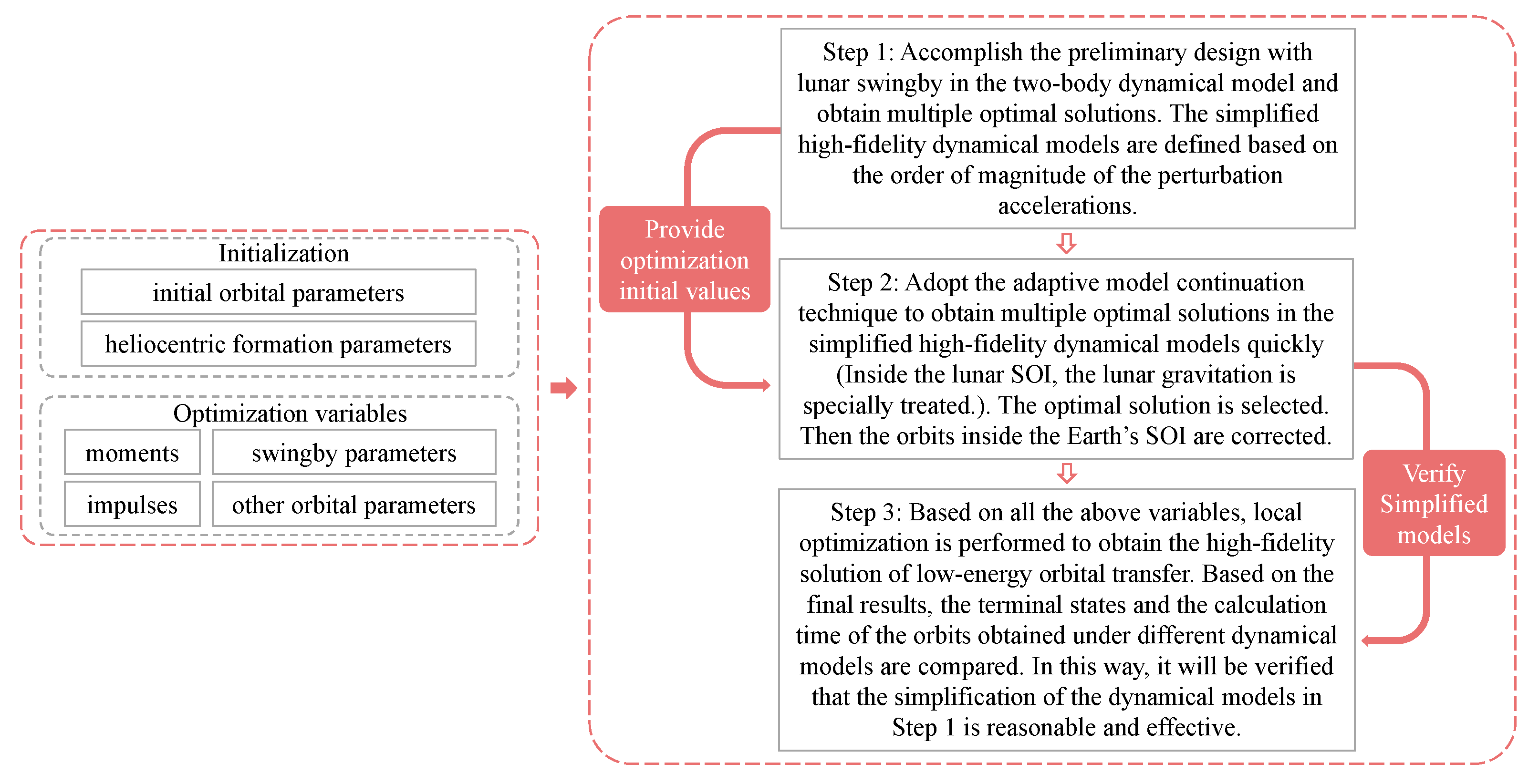
A summary of the design process is presented in a flow chart, as shown in Figure 5. The initial and target orbital parameters are determined based on the existing studies on heliocentric formation. The optimization variables are classified into four classes: time moments, impulses, swingby parameters, and other orbital parameters. The entire design approach consists of three steps.

Step 1: Preliminary design of the transfer orbit in the two-body models. To improve the probability of finding the global optimal solution, the optimization problem is solved in the two-body models first. In these models, the computational efficiency can be greatly improved by using analytic orbital theory and the well-established method of solving the Lambert’s problem [44]. The swingby is equated to an instantaneous impulse and is characterized by two design parameters. The design with the minimum number of impulses is considered first, and then the number of impulses is increased and examined whether the results are better with limited computational resources and acceptable computational times. The solutions are saved for Step 2, and the simplified high-fidelity models are defined based on the order of magnitude of the perturbation accelerations.

The patched-conic approximation is generally applied in the preliminary design for complex trajectory optimization problems. In the patched-conic model, the dynamic environment in this work is assumed to consist of three independent gravitational fields associated with the Earth, Moon, and Sun, respectively, and separated by the Earth’s SOI and the lunar SOI. The orbit of the S/C in a certain SOI is a conic curve without perturbations. When the spacecraft arrives at the SOI, it is necessary to perform the translations expressed by Equation (5) to ensure that the orbit is continuous across the SOI. In the two-body models, if the states of the S/C at the time moment $t_1$ and time moment $t_2$ are given, the velocity increment of the transfer between the two states can be obtained by solving the Lambert’s problem.

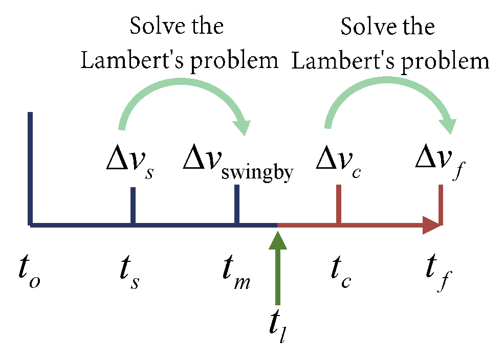
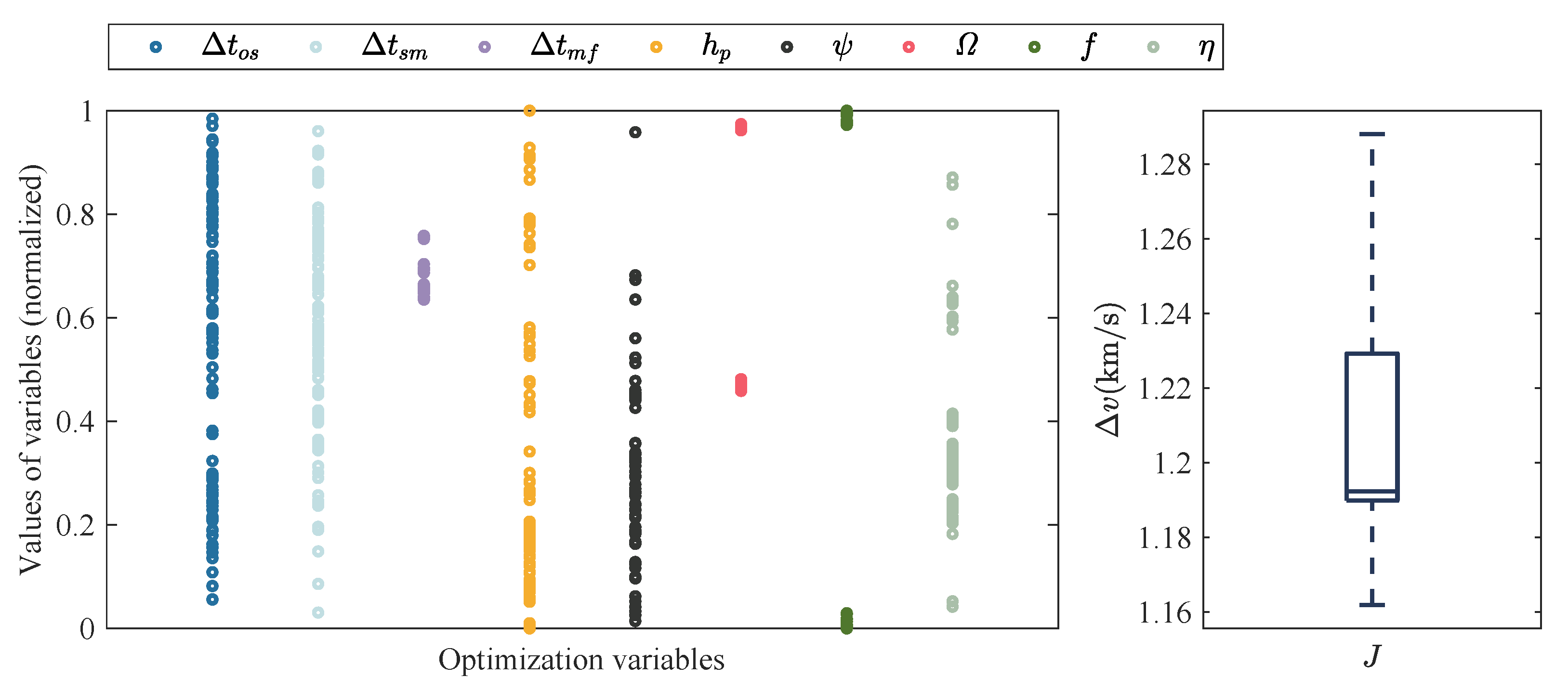
The minimum number of impulses is first applied to achieve lunar swingby and then to rendezvous with the center of the constellation, and an optimization problem with eight variables needs to be solved. Let us denote the start time of the design mission by $t_o$, the start time of the transfer by $t_s$, the time moment of the lunar swingby by $t_m$, and the end time of the transfer by $t_f$. Suppose the S/C leaves the Earth’s SOI at the time moment $t_l$. The eight optimization variables are as follows: the duration from $t_o$ to $t_s$, denoted by $\Delta t_{os}$, the duration from $t_s$ to $t_m$, denoted by $\Delta t_{sm}$, the duration from $t_m$ to $t_f$, denoted by $\Delta t_{mf}$, the lunar swingby altitude and angle, denoted by $h_p$ and $\psi$, respectively, the RAAN of the initial GTO, denoted by $\Omega$, and its true anomaly at the time moment $t_s$, denoted by f, and the scale from 0 to 1 characterizing the time moment of the orbital correction maneuver between $t_l$ and $t_f$, denoted by $\eta$. The time moment of the orbital correction maneuver denoted by $t_c$ is expressed by:

$$t_c=t_l+\eta \left(t_f-t_l\right)$$

(39)

The impulses are applied at $t_s$, $t_c$, and $t_f$, and their magnitude are denoted by $\Delta v_s$, $\Delta v_c$, and $\Delta v_f$, respectively. They are obtained by solving the Lambert’s problem with different revolutions and selecting the solution with the smallest velocity increment. The objective function to be minimized is:

$$minJ=\Delta v_s+\Delta v_c+\Delta v_f$$

(40)

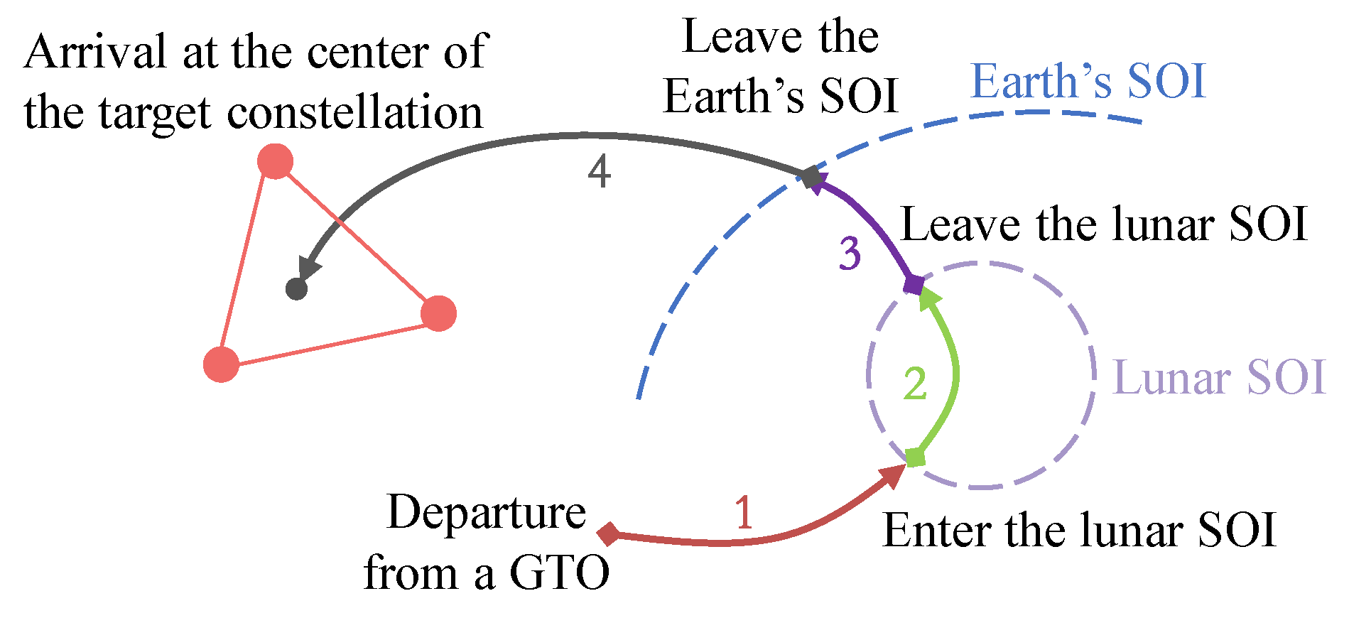
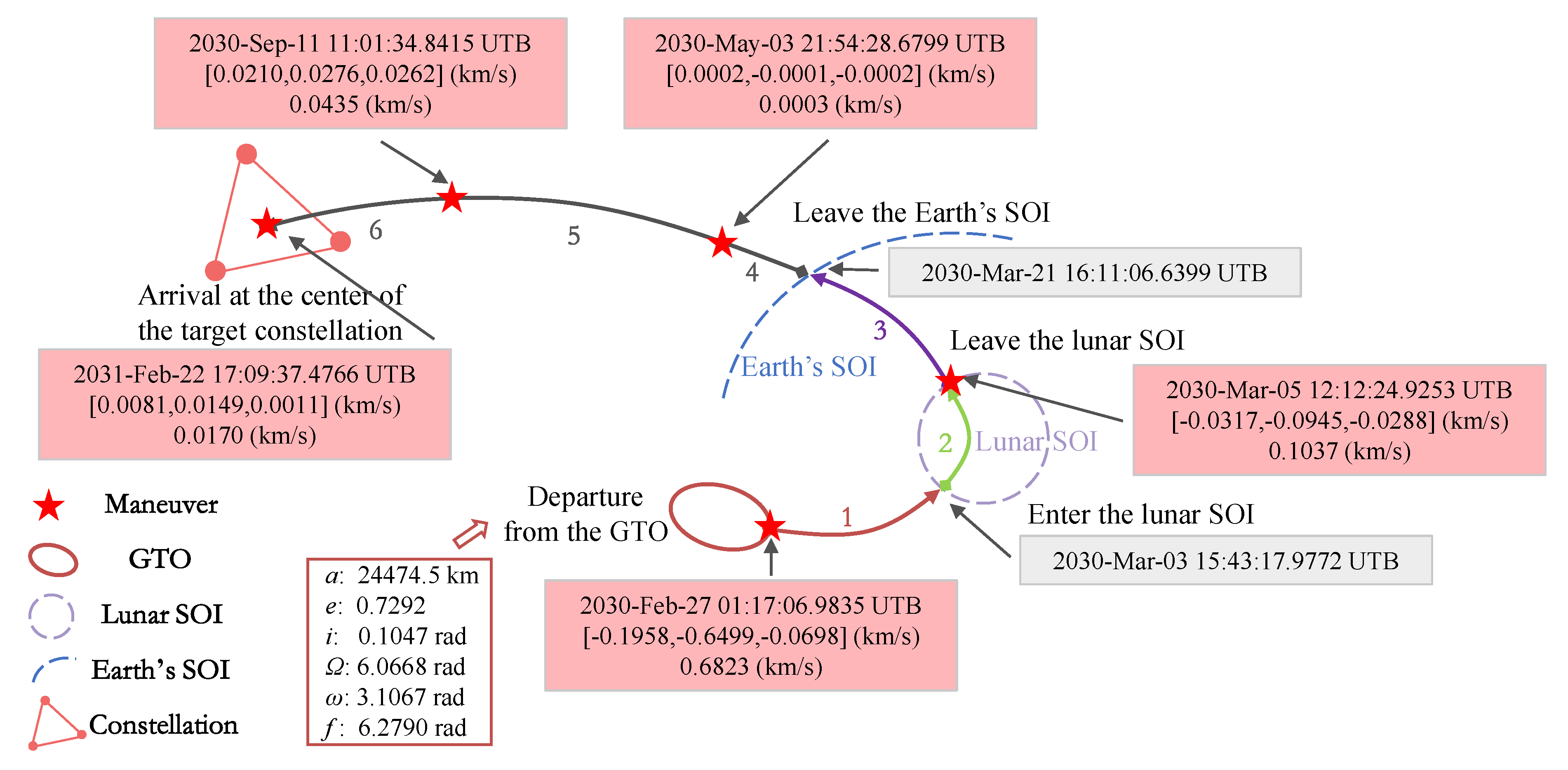
In addition to the initial and final states, the constraints include: (1) The spacecraft should fly by the Moon at the time moment $t_m$; (2) The total transfer duration should be less than the time limit $T_{max}$. The transfer process of the S/C is shown in Figure 6. The blue part is the geocentric orbits, and the red is the heliocentric orbits. The translations from the J2000 ECI frame to the HERF are completed at the boundary of the Earth’s SOI at the time moment $t_l$, which are expressed by Equation (5). The equations of motion of the S/C changes from Equation (9) to Equation (17) without perturbations. The orbits with the time intervals from $t_s$ to $t_m$ and $t_c$ to $t_f$ are obtained by solving the Lambert’s problem, and the remaining orbits are obtained by calculating the equations of motion under the two-body models.

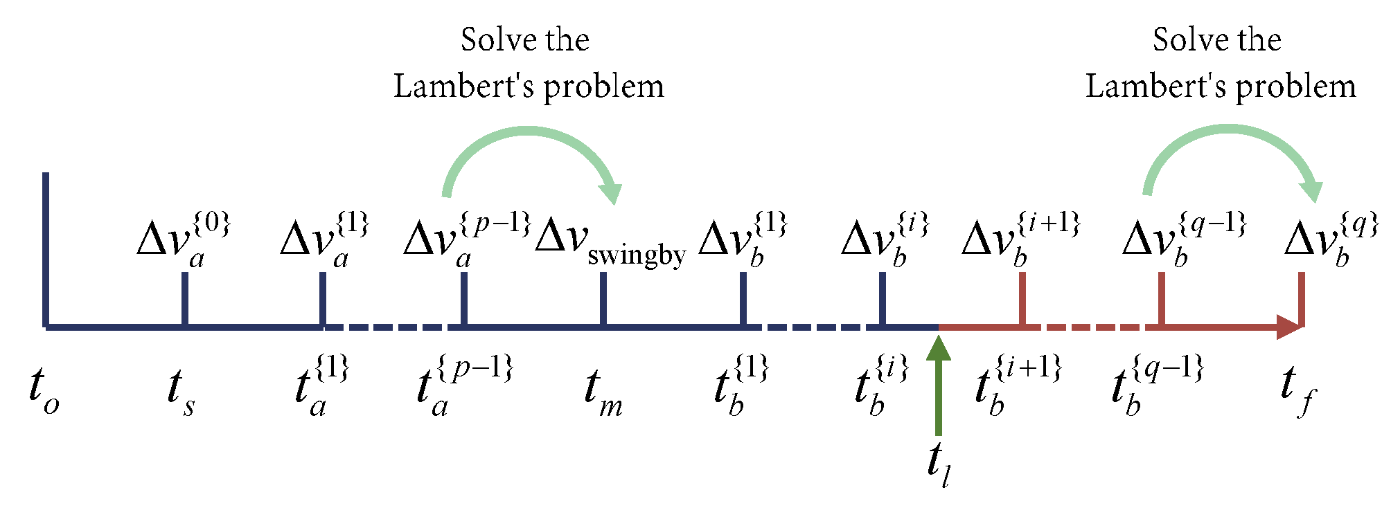
Based on the above calculations, the multi-impulse transfer model will be attempted next, as shown in Figure 7. The number of impulses applied from $t_s$ to $t_m$ is $p\left(p⩾1\right)$, and the number of impulses applied from $t_m$ to $t_f$ is $q\left(q⩾2\right)$. Compared with the minimum impulse number transfer model, some optimization variables are added including: $\Delta {\mathit{v}}_a^{\left\{0\right\}}$, ⋯, $\Delta {\mathit{v}}_a^{\{p-2\}}$, $t_a^{\left\{1\right\}}$, ⋯, $t_a^{\{p-1\}}$, $\Delta {\mathit{v}}_b^{\left\{1\right\}}$, ⋯, $\Delta {\mathit{v}}_b^{\{q-2\}}$, $t_b^{\left\{1\right\}}$, ⋯, and $t_b^{\{q-2\}}$. The transfer orbits from $t_a^{\{p-1\}}$ to $t_m$ and from $t_b^{\{q-1\}}$ to $t_f$ are obtained by solving the Lambert’s problem.

The subsequent numerical experiments will illustrate that the transfer with a total of three maneuvers, as shown in Figure 6, is sufficient in this study. The optimizations are repeated $n_{\mathrm{opt}}$ times in Step 1 to obtain $n_{\mathrm{opt}}$ optimal solutions.

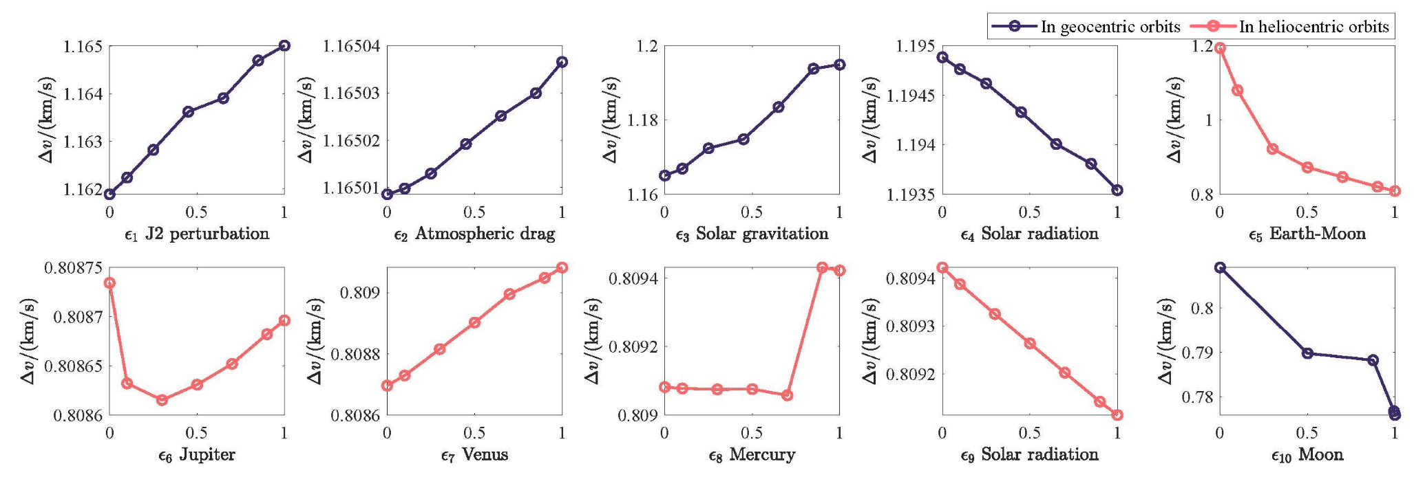
For the high-fidelity models, some of the perturbations are too small to have a discernible effect on the orbit. While the other perturbations must be considered; otherwise, they may lead to significant errors. Therefore, to improve the computational efficiency and keep a small terminal error, it is necessary to retain the perturbations that significantly impact the orbit and ignore those with less impact. Based on the segments of transfer orbit designed in the two-body models, the positions and velocities at multiple discrete time moments on the transfer orbit are obtained. The perturbation accelerations counted into the high-fidelity models of the geocentric and heliocentric orbits are calculated. After normalizing the perturbation accelerations by the central celestial body gravitation acceleration, the simplified high-fidelity models are drawn according to the orders of magnitude and their influences on the terminal states. The final low-energy transfer orbit is refined in these simplified high-fidelity models.

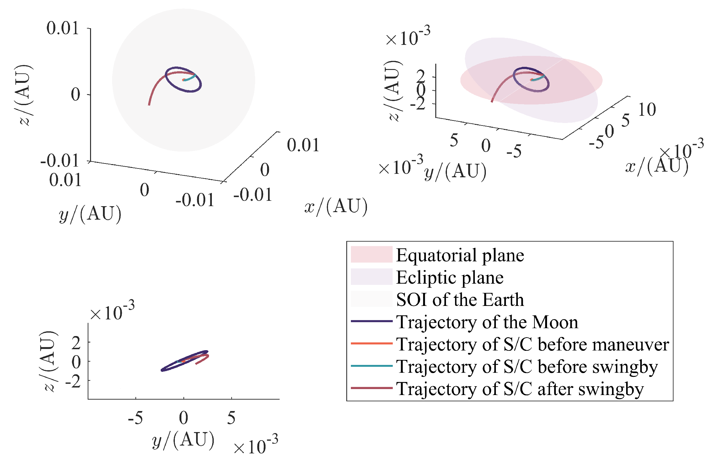
Step 2: Model continuation and swingby correction. This step utilizes the results of Step 1. The $n_{\mathrm{opt}}$ optimal solutions are iterated from the two-body models to the simplified high-fidelity models by the adaptive model continuation technique. The swingby process is specially treated and corrected to obtain approximate orbits in the lunar SOI. Then, the optimal solution among them is picked out. The space size of the lunar SOI and the simplified high-fidelity model of the selenocentric orbits are considered. We maintain the heliocentric orbit unchanged and correct the geocentric orbit. The departure velocity from the GTO is adjusted to shoot the target B-plane parameters. After leaving the lunar SOI, an impulse is added to satisfy the following position constraint at the Earth’s SOI. Finally, another impulse is added at the Earth’s SOI to meet the velocity constraint. In this way, the correction of the geocentric orbit is completed. The details are as follows.

Substep 1: The $n_{\mathrm{opt}}$ optimal solutions are iterated from the two-body models to the approximate simplified high-fidelity models by the adaptive model continuation technique. The lunar gravitation perturbation for the geocentric orbits is still not considered. The lunar swingby is treated as an instantaneous impulse. Each step of the model continuation, corresponding to a change in the model continuation parameter ${ϵ}_i$, solves an optimization problem using a local optimization algorithm. This optimization problem has fourteen variables (include the components of vector variables) as follows: the duration from $t_o$ to $t_s$, denoted by $\Delta t_{os}$, the duration from $t_s$ to $t_m$, denoted by $\Delta t_{sm}$, the duration from $t_m$ to $t_f$, denoted by $\Delta t_{mf}$, the lunar swingby altitude and angle, denoted by $h_p$ and $\psi$, respectively, the RAAN of the initial GTO, denoted by $\Omega$, its true anomaly at the time moment $t_s$, denoted by f, the scale from 0 to 1 characterizing the time moment of the orbital correction maneuver between $t_l$ and $t_f$, denoted by $\eta$, three components of the impulse $\Delta {\mathit{v}}_s$ at the time moment $t_s$, and three components of the impulse $\Delta {\mathit{v}}_c$ at the time moment $t_c$. In the optimization problem, the constraints to be satisfied and the objective function are the same as in the preliminary design. However, since the solution of the two-point boundary-value problem considering the perturbations cannot be obtained by directly solving the Lambert’s problem, the residuals of the position constraints at $t_m$ and $t_f$ are added to the objective function as penalty terms. The order of model continuation that adds the perturbations in turn into the dynamical models is the $J_2$ perturbation of the Earth, atmospheric drag, solar gravitation, and solar radiation for the geocentric orbits, and the gravitation of the Earth–Moon system, Jupiter, Venus, and Mercury, and the solar radiation for the heliocentric orbits.

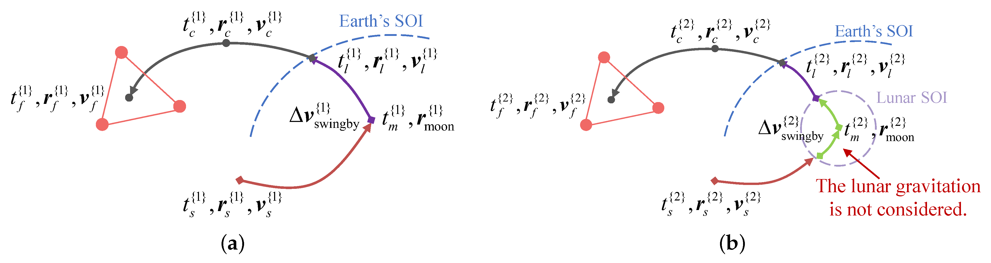
Substep 2: The space size of the lunar SOI is considered, and the lunar gravitation is gradually added to the dynamical model for the geocentric orbits by gradually increasing the continuation parameter. There is a special treatment inside the lunar SOI [45]. When the S/C flies inside the lunar SOI, the lunar gravitation is set to 0. The S/C flies by the Moon at the time moment $t_m$ under the influence of the Earth’s gravitation and other perturbations. At this time moment, the lunar swingby is still equivalent to an instantaneous impulse. Note that the design result of Substep 1 is regarded as the initial value of the optimization problem corresponding to Substep 2. The difference between Substep 1 and Substep 2 is only in the dynamical models. The variables, constraints, and objective function in this optimization problem are the same as described in the immediately preceding paragraph. A schematic diagram of Substeps 1 and 2 is shown in Figure 8, where t, $\mathit{r}$, and $\mathit{v}$ denote the time moments, position vectors, and velocity vectors, respectively, and the subscripts s, m, l, c, and f represent the time moments of the departure from the GTO, the flyby of the Moon, the departure from the Earth’s SOI, the orbital correction, and the arrival at the target position, respectively. The superscripts {1} and {2} are used in subfigures (a) and (b) to distinguish the results of Substeps 1 and 2, respectively.

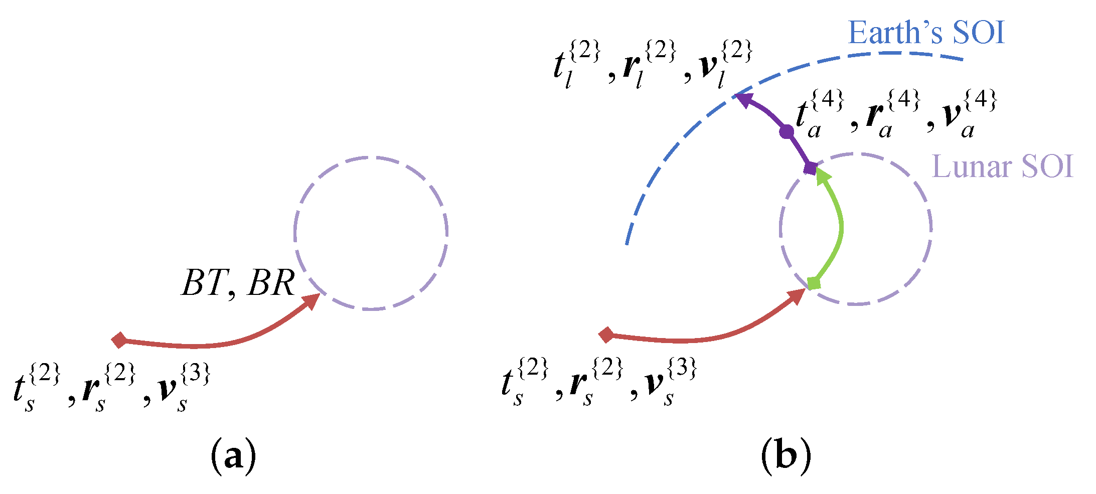
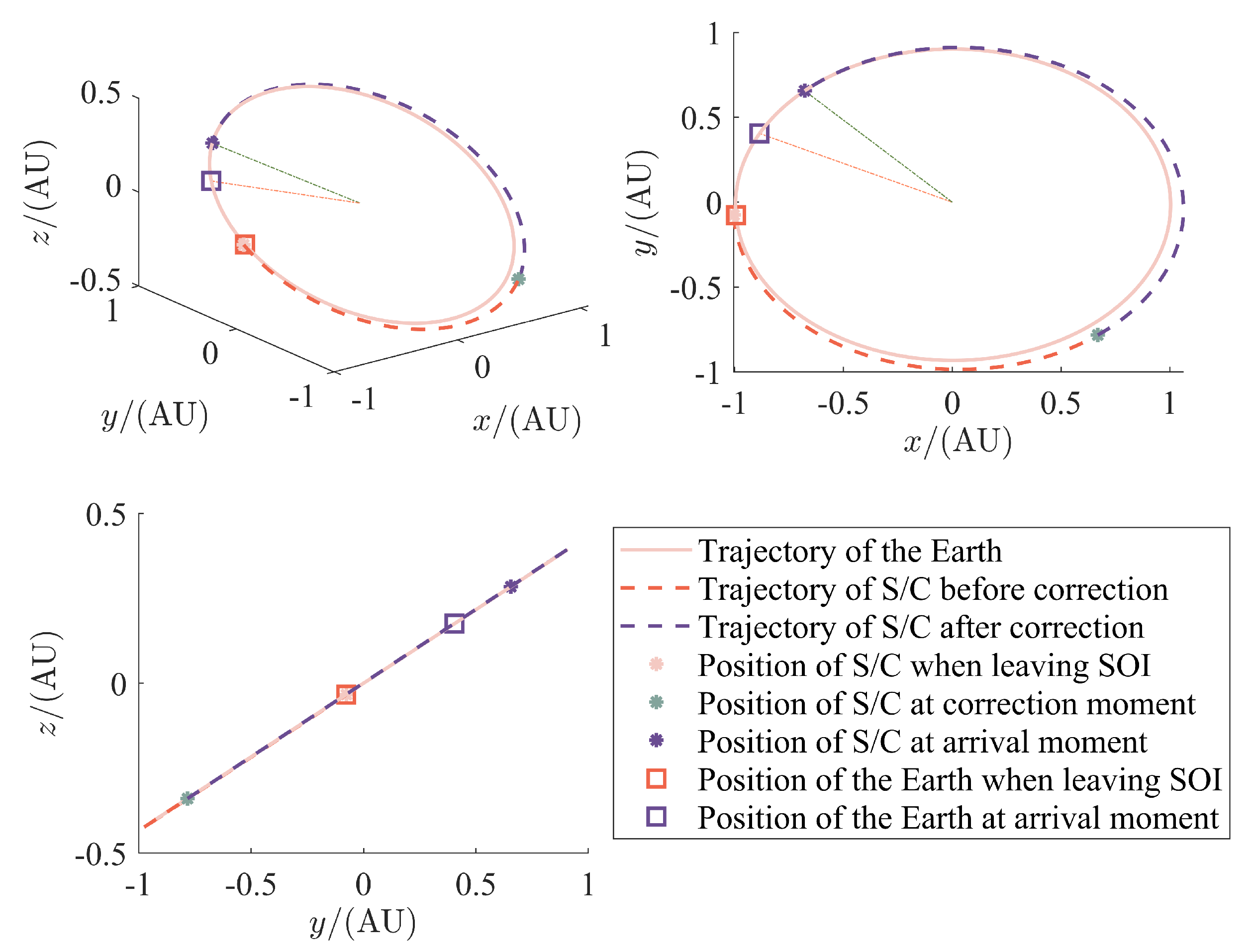
Substep 3: The optimal solution among $n_{\mathrm{opt}}$ solutions in Substep 2 is picked out to complete the subsequent design. We maintain the heliocentric orbit unchanged and correct the geocentric orbit. This means that the time moment of arrival at the Earth’s SOI and the corresponding position and velocity remain the same as the design result of Substep 2. In the above substeps, the lunar swingby effect is equivalent to an instantaneous impulse, and the orbit inside the lunar SOI is approximate. Therefore the departure velocity from the GTO needs to be corrected to achieve the desired lunar swingby effect. The B-plane parameters $BT$ and $BR$ are used to correct the impulse at the departure time moment $t_s$ as mentioned in Section 3.1. This requires shooting the nonlinear Equation (37). After the correction, the S/C still cannot reach the position of the Earth’s SOI designed in the previous step at the time moment $t_l$. The time moment of leaving the lunar SOI is denoted by $t_{m2}$. A correction impulse is added in the orbit during the time moment $t_{m2}$ to the time moment $t_l$. Another impulse is added at the time moment $t_l$ to meet the velocity requirement. The two impulses are denoted by $\Delta {\mathit{v}}_a$ and $\Delta {\mathit{v}}_b$, and the corresponding time moments are denoted by $t_a$ and $t_b$, where $t_b=t_l$. The schematic diagram of Substep 3 is shown in Figure 9, where the subscript a represents the time moment of the orbital correction between $t_{m2}$ and $t_l$, and the rest symbols have the same meaning as in Figure 8. The superscripts {3} and {4} are used in subfigures (a) and (b) to distinguish the results after shooting the B-plane parameters and adding two correction impulses in Substep 3. Note that when the superscripts of the symbols in Figure 8 and Figure 9 are the same, their values are the same.

Step 3: Local optimization and validation of the simplified dynamical models. A local optimization problem should be solved. It has twenty optimization variables, twelve from Substep 1 of Step 2 (except for the swingby parameters $r_p$ and $\psi$) and eight from the swingby correction ($t_a$, $t_b$, and six components of $\Delta {\mathit{v}}_a$ and $\Delta {\mathit{v}}_b$ in total). The ranges of the optimization variables are kept unchanged. The objective function to be minimized is:

$$minJ=\Delta v_s+\Delta v_c+\Delta v_a+\Delta v_b+\Delta v_f$$

(41)

where $\Delta v_a$ and $\Delta v_b$ are the magnitude of $\Delta {\mathit{v}}_a$ and $\Delta {\mathit{v}}_b$, respectively, and the rest of the symbols have the same physical meaning as in Equation (40). The states at the initial and final time moments need to be satisfied, and the total transfer duration should be less than the time limit $T_{\max }$. Then, the simplified high-fidelity solution of low-energy orbital transfer is obtained by local optimization. As mentioned in Section 2, for the geocentric orbits, in addition to the central gravitation of the Earth, the orbit of the spacecraft is affected by the perturbations due to the Earth’s nonspherical gravitation, atmospheric drag, solar gravitation, lunar gravitation, solar radiation, relativistic effects, solid tides, ocean tides, Earth’s rotational deformation, etc. For the heliocentric orbits, in addition to the solar gravitation, the orbit of the spacecraft is affected by the perturbations due to the gravitation of Mercury, Venus, Earth, Mars, Jupiter, Saturn, Uranus, Neptune, Pluto, the Moon, the solar radiation, etc. In the simplified high-fidelity models, the perturbations due to the Earth’s nonspherical gravitation, atmospheric drag, lunar gravitation, solar gravitation, and solar radiation are considered for the geocentric orbits, and the perturbations due to the gravitation of the Earth–Moon system, Jupiter, Venus, and Mercury, and the solar radiation are considered for the heliocentric orbits. Based on the design results in Step 2, we can calculate the terminal position and velocity relative errors obtained by integrating the equations of motion in the high-fidelity dynamical models and simplified high-fidelity models and record the computational times spent on propagating a single orbit. We will further verify that simplifying the dynamical models is reasonable and effective. The relative errors of terminal position and velocity and the ratio of computational times between the model j and the model i are defined as:

$$e_r=\frac{∥{\mathit{r}}_j-{\mathit{r}}_i∥}{∥{\mathit{r}}_i∥},e_v=\frac{∥{\mathit{v}}_j-{\mathit{v}}_i∥}{∥{\mathit{v}}_i∥},c_t=\frac{t_{\mathrm{cost}\mathrm{j}}}{t_{\mathrm{cost}\mathrm{i}}}$$

(42)

where ${\mathit{r}}_j$, ${\mathit{v}}_j$, and $t_{\mathrm{cost}\mathrm{j}}$ denote the terminal position and velocity and computational times of propagating a single orbit under the model j, respectively, and ${\mathit{r}}_i$, ${\mathit{v}}_i$, and $t_{\mathrm{cost}\mathrm{i}}$ denote those under the model i, respectively. Smaller $e_r$ and $e_v$ means that the two models are close to each other, and smaller $c_t$ means that it takes a shorter time to propagate the orbit under the model j.

4. Results and Discussion

1 January 2030, is chosen as the start time of the designed mission, which is denoted by $t_o$ as stated before. The duration of the transfer is limited to 540 days. The start orbit of the transfer is set to the GTO launched by the Ariane 5 [32], and the orbital parameters are shown in

Table 4. Orbital parameters of the GTO.

Orbital Parameters	Value	Unit
Inclination	6	degree
Altitude of perigee	250	km
Altitude of apogee	35,943	km
Argument of perigee	178	degree

. The right ascension of ascending node and the true anomaly at the initial time moment of the transfer are considered as optimization variables. The planetary and lunar ephemerides are obtained from the DE430 ephemeris of JPL [34].

The example of LISA is simulated to demonstrate the presented design approach. The specific implementation details, results, and analysis of the three parts of the design approach are described in turn.

4.1. Preliminary Design in Two-Body Dynamical Models

First, a global optimization algorithm is utilized to find the global optimal solution as well as possible in the two-body models. The minimum number of impulses is first investigated, and the ranges of the eight variables are shown in

Table 5. Ranges of optimization variables.

Variables	Lower Bound	Upper Bound	Unit
$\Delta t_{os}$	0.0	12.0	month
$\Delta t_{sm}$	0.0	6.0	month
$\Delta t_{mf}$	0.0	16.0	month
$h_p$	200	1000	km
$\psi$	0.0	2$\mathsf{\pi }$	rad
$\Omega$	0.0	2$\mathsf{\pi }$	rad
f	0.0	2$\mathsf{\pi }$	rad
$\eta$	0.0	1.0	/

.

The particle swarm optimization (PSO) algorithm [46] is adopted to solve the optimization problem of preliminary design, which is a stochastic search algorithm based on population collaboration developed by simulating the foraging behavior of a flock of birds. Each particle is regarded as a search individual in the N-dimensional space, and the current position of the particle is a candidate solution to the corresponding optimization problem. The velocity of the particle is dynamically adjusted according to the historical optimal position of the particle and the historical optimal position of the swarm. The PSO algorithm balances the global and local search through parameters. It does not need to calculate the gradient and is widely used in trajectory optimization problems because of its fast convergence speed and strong versatility. The parameter setting of the PSO algorithm in this work is referred to Jiang et al. [47]. As the number of iterations increases, the inertia factor $\omega$ decreases linearly from 0.9 to 0.4, and the self-confidence $c_1$ and swarm confidence $c_2$ decreases linearly from 2.5 to 0.5, respectively. The maximal velocity $V_{max}$ is 0.8.

To speed up the computational efficiency, we adopt a multi-core parallel technique and use a technique of discrete storage and linear interpolation for the Earth and the Moon ephemerides. The positions and velocities of the Earth and the Moon are obtained from the JPL’s DE430 [34], with the Earth ephemerides stored with step size 0.01 day and the Moon ephemerides stored with step size 0.005 day. All variables are normalized to $[0,1]$ according to their upper and lower bounds when using the PSO algorithm. In this work, the swarm size is set to 5000, the maximal iteration number is set to 5000, and the optimization is repeated 100×. All the tests are run on an Intel Core i9-12900K Processor with 16 cores and 24 threads at 3.0 GHz. The program is run on the C++ platform.

The optimization program is run 100 times independently according to the parameter setting of the PSO algorithm above, and the consequent 100 optimal solutions are recorded. They are shown in Figure 10, which depicts the values of optimization variables and the total velocity increments as the objective function J. We use a boxplot to measure the dispersion of J. Among the 100 independent solutions, the values of $\Delta t_{mf}$, $\Omega$, and f are more concentrated. After denormalization, the average value of $\Delta t_{mf}$ is 321.3093 days, $\Omega$ is concentrated around 6.0665 rad and 2.9515 rad, and f is concentrated around 0.0038 rad. The values of the other variables are distributed in [0, 1] without obvious aggregation. As for the velocity increments of the 100 solutions, the maximum is 1.2880 km/s, the minimum is 1.1619 km/s, the mean is 1.2092 km/s, and the standard deviation is 0.0276 km/s. All optimization variables of the best solution are shown in

Table 6. Values of optimization variables in the two-body dynamical models.

Results	Value	Unit
$\Delta t_{os}$	57.0635	day
$\Delta t_{sm}$	5.5817	day
$\Delta t_{mf}$	355.1359	day
$h_p$	655.9315	km
$\psi$	1.9007	rad
$\Omega$	6.0780	rad
f	6.2648	rad
$\eta$	0.4100	/

and

Table 7. Magnitudes of maneuver and swingby impulses in the two-body dynamical models.

Results	Value	Unit
$\Delta v_s$	0.6783	km/s
$\Delta v_c$	0.0036	km/s
$\Delta v_f$	0.4799	km/s
$\Delta v_{\mathrm{swingby}}$	1.2527	km/s

, where $\Delta v_{\mathrm{swingby}}$ is the velocity increment due to the lunar swingby. The total transfer duration is 360.7176 days and the total velocity increment to be provided by the engine is 1.1619 km/s. The geocentric and heliocentric trajectories are shown in Figure 11 and Figure 12.

Then, the multi-impulse transfer model is investigated. An optimization problem is constructed for the multi-impulse model with the optimization variables, objective function, and constraints as described in Section 3.3. The following two approaches are tried: (1) Directly search for the optimal solution of the optimization problem with the multi-impulse transfer model using the global optimization algorithm, i.e., the PSO algorithm. (2) locally optimize the problem using the local optimization algorithm library NLopt [48]. The solution corresponding to the minimum impulse number model is regarded as the initial value for solving this optimization problem. NLopt is a general library of optimization algorithms for nonlinear optimization, containing a variety of global and local optimization algorithms that can solve unconstrained and constrained optimization problems and handle nonlinear and inequality constraints. According to the calculation, the total velocity increment corresponding to the multi-impulse model is not significantly better than that corresponding to the minimum impulse number transfer model. Therefore, we finally adopted the transfer design with three maneuvers in the preliminary design.

The perturbation accelerations counted into the high-fidelity models are calculated based on the states on the transfer orbit obtained under the two-body models. The parameters of the high-fidelity models are as follows. For the geocentric orbits, the EGM96 [49] is used to model the nonspherical gravitation perturbation, and the highest order of the spherical harmonic coefficients is set to 20. For the atmospheric drag, the drag coefficient is set to 2.2, and the area-mass ratio of the S/C is set to 0.01. The atmospheric density at a certain point is calculated by linear interpolation with the 1976 standard atmosphere model [50]. For the solar and lunar gravitation perturbations, the accelerations are calculated according to the third-body gravitation model. For the solar radiation acceleration, the solar radiation coefficient is 1.5, the speed of light is $2.99792458\times {10}^8$ m/s, and the luminosity of the Sun is $3.823\times {10}^{26}$ W. A cylindrical ground shadow model is used, which regards sunlight as parallel light. In addition to the above perturbations, relativistic effects, solid tides, ocean tides, and the Earth’s rotational deformation are also considered. As for the relativistic effects, only the first-order post-Newtonian effect is considered, which is the largest one. For the heliocentric orbits, the perturbation accelerations of the gravitation of the Mercury, Venus, Earth, Moon, Mars, Jupiter, Saturn, Uranus, Neptune, and Pluto, and the solar radiation are considered. The ranges of the order of magnitude of the above perturbation accelerations along the 1st, 3rd, and 4th orbit segments in Figure 2 are estimated (normalized by the central gravitation of the Earth), as shown in

Table 8. Orders of magnitude of the perturbation accelerations for the geocentric orbits.

Accelerations (Normalized)	1st	3rd
Lunar gravitation 1	${10}^{-7}$∼${10}^0$	${10}^{-5}$∼${10}^0$
Nonspherical gravitation	${10}^{-9}$∼${10}^{-2}$	${10}^{-12}$∼${10}^{-9}$
Atmospheric drag	$0\sim {10}^{-5}$	0
Solar gravitation 2	${10}^{-7}$∼${10}^{-5}$	${10}^{-5}$∼${10}^0$
Solar radiation	${10}^{-8}$	${10}^{-8}$
Relativistic effects	${10}^{-13}$∼${10}^{-8}$	${10}^{-15}$∼${10}^{-13}$
Solid tides	${10}^{-14}$∼${10}^{-7}$	${10}^{-17}$∼${10}^{-13}$
Ocean tides	${10}^{-15}$∼${10}^{-8}$	${10}^{-18}$∼${10}^{-15}$
Rotation deformation	${10}^{-18}$∼${10}^{-9}$	${10}^{-20}$∼${10}^{-15}$

¹ At the lunar SOI, the lunar gravitation acceleration is of the same order of magnitude as the Earth’s gravitation acceleration. ² At the Earth’s SOI, the solar gravitation acceleration is of the same order of magnitude as the Earth’s gravitation acceleration.

and

Table 9. Orders of magnitude of the perturbation accelerations for the heliocentric orbits.

Accelerations (Normalized)	4th
Earth gravitation 1	${10}^{-7}$∼${10}^0$
Lunar gravitation	${10}^{-9}$∼${10}^{-2}$
Jupiter gravitation	${10}^{-8}$∼${10}^{-7}$
Solar radiation	${10}^{-8}$
Venus gravitation	${10}^{-8}$
Mercury gravitation	${10}^{-9}$∼${10}^{-8}$
Saturn gravitation	${10}^{-9}$
Mars gravitation	${10}^{-10}$
Uranus gravitation	${10}^{-11}$
Neptune gravitation	${10}^{-11}$
Pluto gravitation	${10}^{-16}$∼${10}^{-15}$

¹ At the Earth’s SOI, the solar gravitation acceleration is of the same order of magnitude as the Earth’s gravitation acceleration.

. According to the orders of magnitude of the perturbation accelerations and the error in the terminal state of the transfer orbit calculated under different dynamical models, the perturbations of the Earth’s nonspherical gravitation, atmospheric drag, lunar gravitation, solar gravitation, and solar radiation are considered for the geocentric orbits; meanwhile, the perturbations of the gravitation of the Earth–Moon system, Jupiter, Venus, and Mercury, and the solar radiation are considered for the heliocentric orbits. When we design the transfer orbit, the dynamical model of the selenocentric orbits is required only in the last step, at which the lunar swingby is corrected. Moreover, the flight time of the S/C in the lunar SOI is relatively short. Therefore, considering that the perturbation accelerations of the Earth’s nonspherical gravitation and atmospheric drag as far as the Moon are too weak to consider, only the gravitation of the Moon, Earth, and Sun, and the solar radiation are adopted into the equations of motion on the selenocentric orbits.

The simplified models are effective in balancing the computational accuracy and computational efficiency. To support this simplification, we will verify the accuracy and efficiency in Section 4.3.

4.2. Adaptive Model Continuation and Swingby Correction

As described in Section 3.3, three substeps are required to complete the model continuation and swingby correction. In Substep 1, $n_{\mathrm{opt}}$ optimal solutions are iterated from the two-body models to the approximate simplified high-fidelity models by the adaptive model continuation technique, where for the geocentric orbits, only the lunar gravitation perturbation is not considered. The lunar swingby is treated as an instantaneous impulse. This substep entails solving a series of optimization problems based on the adaptive model continuation technique. As mentioned before, this series of optimization problems has fourteen optimization variables, six of which are impulse components that have values between −1 km/s and 1 km/s. The ranges of the other optimization variables are shown in Table 5. The values of the optimization variables obtained in Section 4.1 and the values of the impulses obtained by solving the corresponding Lambert’s problem constitute the initial values for this substep. The order of model continuation that adds the perturbations in turn into the dynamical models is the $J_2$ perturbation of the Earth, atmospheric drag, solar gravitation, and solar radiation for the geocentric orbits, and the gravitation of the Earth–Moon system, Jupiter, Venus, and Mercury, and the solar radiation for the heliocentric orbits. In our simulation, for each perturbation, the initial step size is 0.1, the decline rate is 0.5, and the growth rates are 1.5 and 2.0 for the geocentric and heliocentric orbits, respectively. The maximum step size does not exceed 0.2, and the convergence judgment parameter is 0.01.

In Substep 2, add the lunar gravitation perturbation when propagating the geocentric orbits outside the lunar SOI. Inside the lunar SOI, the lunar gravitation is not considered, and the lunar swingby effect is still equivalent to an instantaneous impulse. In this substep, the lunar gravitation is gradually added to the dynamical models by the adaptive model continuation technique, corresponding to solving a series of optimization problems. In the series of optimization problems, the optimization variables along with their ranges and the expressions of the objective functions and constraints are the same as in Substep 1, and their initial values are adopted from the solutions of Substep 1. In this simulation, the initial step size is 0.2, the decline rate is 0.5, the growth rate is 2.0, the maximum step size is 0.2, and the convergence judgment parameter is 0.01.

The best of the $n_{\mathrm{opt}}$ solutions obtained after Substep 1 and Substep 2 is picked out for the subsequent corrections. The results of Substep 1 and Substep 2 are shown in Figure 13, where each subplot represents a model continuation process of one perturbation, where ${ϵ}_i,i=1,\cdots ,10$ represent, for the geocentric orbits, the $J_2$ perturbation, atmospheric drag, solar gravitation, and solar radiation, for the heliocentric orbits, the gravitation of the Earth–Moon system, Jupiter, Venus, and Mercury, and the solar radiation, and for the geocentric orbits, the lunar gravitation, respectively. The points of each subplot indicate the convergent solutions, the horizontal coordinate indicates the value of ${ϵ}_i$ at convergence, which is calculated by the adaptive model continuation technique, and the vertical coordinate indicates the corresponding velocity increment. The parameter values also affect the final result. Too large a step size may produce poor optimization results due to underutilization of the perturbation, which is essentially caused by jumping out of the current local optimal solution. The change in velocity increment after increasing the corresponding model continuation parameter from 0 to 1 for each perturbation is collated in

Table 10. Changes of velocity increment in model continuation.

	Perturbation	Increase or Decrease	Value (km/s)
In geocentric orbits	$J_2$ perturbation	+	$3.1157\times {10}^{-3}$
	Atmospheric drag	+	$2.7970\times {10}^{-5}$
	Solar gravitation	+	$2.9845\times {10}^{-2}$
	Solar radiation	−	$1.3405\times {10}^{-3}$
In heliocentric orbits	Earth-Moon system gravitation	−	$3.8481\times {10}^{-1}$
	Jupiter gravitation	−	$3.8132\times {10}^{-5}$
	Venus gravitation	+	$3.8555\times {10}^{-4}$
	Mercury gravitation	+	$3.4022\times {10}^{-4}$
	Solar radiation	−	$3.0718\times {10}^{-4}$
In geocentric orbits	Lunar gravitation	−	$3.3302\times {10}^{-2}$

, where + indicates an increase in velocity increment and − indicates a decrease. The most significant effect on the transfer velocity increment is due to the gravitation of the Earth–Moon system for the heliocentric orbits, and the velocity increment decreases from 1.1935 km/s to 0.8087 km/s after adding it. Except for this, the solar and lunar gravitation for the geocentric orbits has large effects on the change of velocity increment. The other perturbations cause changes in velocity increment below 0.01 km/s. The gravitation of the Earth–Moon system, Jupiter, and Moon, and the solar radiation help reduce the velocity increment required for the transfer. It is inferred that it is necessary to consider the simplified high-fidelity models in the transfer design. It is worth noting that the change of velocity increment after considering the lunar gravitation for the geocentric orbits is small. Combined with the subsequent correction results, it is shown that equating the swingby effect with an instantaneous impulse in the preliminary design is reasonable and accurate, which may provide a good initial value for the subsequent design.

The values of all optimization variables and the magnitudes of the impulses of the best solution are shown in

Table 11. Values of optimization variables after Substep 1 and Substep 2.

Results	Value	Unit
$\Delta t_{os}$	57.0529	day
$\Delta t_{sm}$	5.4528	day
$\Delta t_{mf}$	355.4343	day
$h_p$	232.6900	km
$\psi$	1.7544	rad
$\Omega$	6.0668	rad
f	6.2792	rad
$\eta$	0.4809	/
$v_{sx}$	−0.1301	km/s
$v_{sy}$	−0.6661	km/s
$v_{sz}$	−0.0698	km/s
$v_{cx}$	0.0323	km/s
$v_{cy}$	0.0352	km/s
$v_{cz}$	0.0275	km/s

and

Table 12. Magnitudes of maneuver and swingby impulses after Substep 1 and Substep 2.

Results	Value	Unit
$\Delta v_s$	0.6822	km/s
$\Delta v_c$	0.0551	km/s
$\Delta v_f$	0.0385	km/s
$\Delta v_{\mathrm{swingby}}$	1.3677	km/s

, where $\Delta v_{\mathrm{swingby}}$ is the velocity increment due to the lunar swingby. The total transfer duration is 360.8871 days and the total velocity increment to be provided by the engine is 0.7758 km/s. Comparing the values of the velocity increments in Table 7 and Table 12, the main change is in $\Delta v_f$, indicating that the addition of the perturbations reduces the magnitude of the propulsive impulse at the terminal time moment.

Then, the orbit inside the Earth’s SOI is corrected by Substep 3. The solution of Substep 2 includes the position and velocity corresponding to the departure time moment $t_s$ of the spacecraft, the position and velocity corresponding to the time moment $t_l$ of leaving the Earth’s SOI, and the swingby parameters $r_p$ and $\psi$. The position and velocity corresponding to the time moment $t_l$ should be the same as the corresponding values in Substep2. The target B-plane parameters $B{T}_t$ and $B{R}_t$ are calculated using the the swingby parameters $r_p$ and $\psi$. Maintaining the departure time moment and the corresponding position unchanged, the actual B-plane parameters $B{T}_a$ and $B{R}_a$ of the spacecraft when it reaches the lunar SOI are made as close to the target B-plane parameters by adjusting the two components of the corresponding velocity as possible. This requires solving the system of binary nonlinear equations, as described in Equation (37). The corresponding system of equations with $[\Delta v_{sx},\Delta v_{sy}]$, $[\Delta v_{sx},\Delta v_{sz}]$, and $[\Delta v_{sy},\Delta v_{sz}]$ as three sets of variables are solved, respectively. Combining the results of the two correction impulses in subsequent calculations, the solution with the smallest increase in velocity increment is chosen. MinPack-1 [51], a package of FORTRAN subprograms for solving nonlinear equations and nonlinear least squares problems, is used to solve Equation (37). It is a widely used and relatively well-developed package in which the section on solving nonlinear equations has been translated into C++ programming language in our simulations. In the problem of shooting the B-plane parameters, the relationships between $BT$ and $BR$ and the initial velocity are nearly linear, and the solving of nonlinear equations converges after a few iterations. Then, the velocity at the time moment of departure is updated according to the solution of the nonlinear equations, and the time moment, position, and velocity of the spacecraft when it leaves the lunar SOI are obtained. The addition of an impulse at a suitable time moment after leaving the lunar SOI enables the spacecraft to meet the position at the time moment $t_l$ designed in Substep 2. This impulse is denoted by $\Delta {\mathit{v}}_a$. An impulse is applied at the time moment $t_l$ to meet the velocity at the time moment $t_l$ designed in Substep 2. This impulse is denoted by $\Delta {\mathit{v}}_b$.

The results corresponding to the three sets of optimization variables $[\Delta v_{sx},\Delta v_{sy}]$, $[\Delta v_{sx},\Delta v_{sz}]$, and $[\Delta v_{sy},\Delta v_{sz}]$ are listed in

Table 13. Results of swingby correction.

Variables	$[{\mathit{BT}}_{\mathit{t}},{\mathit{BR}}_{\mathit{t}}]$ (km)	$\mathbf{\Delta }{\mathit{v}}_{\mathit{s},0}$ (km/s)	$[{\mathit{BT}}_{\mathit{a}},{\mathit{BR}}_{\mathit{a}}]$ (km)	$\mathbf{\Delta }{\mathit{v}}_{\mathit{s}}$ (km/s)	$\mathbf{\Delta }{\mathit{v}}_{\mathit{a}}$ (km/s)	$\mathbf{\Delta }{\mathit{v}}_{\mathit{b}}$ (km/s)	$\mathbf{\Delta }{\mathit{v}}_{\mathbf{tot}}$ (km/s)
$[\Delta v_{sx},\Delta v_{sy}]$	[−4688.26, −2255.5]	0.6822	[−4687.9280, −2255.5854]	0.6823	0.1697	0.0151	0.1849
$[\Delta v_{sx},\Delta v_{sz}]$			[−4688.2573, −2255.5030]	0.7049	0.1678	0.0152	0.2057
$[\Delta v_{sy},\Delta v_{sz}]$			[−4870.1398, −468.9880] 1	0.6832	0.1385	0.0957	0.2352

¹ Solving the system of nonlinear equations is not successful.

, where $[B{T}_t,B{R}_t]$ and $[B{T}_a,B{R}_a]$ denote the target and actual B-plane parameters after shooting, respectively, $\Delta v_{s,0}$ denotes the magnitude of the impulse at departure in Substep 2, $\Delta v_s$, $\Delta v_a$, and $\Delta v_b$ denote the magnitudes of the impulses at the departure time moment, at the first correction time moment, and at the second correction time moment, respectively, and $\Delta v_{\mathrm{tot}}$ denotes the increased velocity increment in Substep 3 compared with the result of Substep 2. It is worth noting that the increased velocity increment differences between the three sets of optimization variables are not large. Exceptionally, when $[\Delta v_{sy},\Delta v_{sz}]$ are used as the optimization variables, even the shooting Equation (37) does not converge, the increased velocity increment still is little. This further illustrates that it is feasible to equate the lunar swingby with an instantaneous impulse in the preliminary design, but the error is not negligible. The results corresponding to $[\Delta v_{sx},\Delta v_{sy}]$ are adopted for the subsequent design.

4.3. Local Optimization and Validation of Simplified Dynamical Models

Based on the above simulation results and analyses, a local optimization with twenty variables is performed to obtain the high-fidelity solution of low-energy orbital transfer, which is solved by NLopt. We present the low-energy orbital transfer design result in Figure 14, which shows the initial orbital parameters, the time moment of each impulse and its component and magnitude, the time moments of entry and escape from the lunar SOI, and the time moment of escape from the Earth’s SOI. The transfer requires a velocity increment of 0.8468 km/s from the engine and a total transfer time of 360.6615 days.

Finally, we compare the terminal states obtained under the two-body dynamical models, the simplified high-fidelity dynamical models, and the high-fidelity dynamical models with the same initial state and record their computational times of propagating a single orbit segment. The relative errors in position and velocity and the ratios of computational times of the results under different dynamical models with respect to the results under the high-fidelity models are calculated separately and denoted by $[e_r,e_v,c_t]$. The parameters of the high-fidelity dynamical models are the same as those described in Section 4.1. We use the initial and final time moments and the initial states of the 1st, 3rd, and 5th orbits in Figure 14 to obtain $[e_r,e_v,c_t]$ under different models relative to the high-fidelity models, collated in

Table 14. Relative errors in terminal states and ratios of computational times under different models.

Orbit	Two-Body Dynamical Models	Simplified High-Fidelity Dynamical Models
1	$[2.7063\times {10}^{-2},4.9719\times {10}^{-1},2.8986\times {10}^{-6}]$	$[2.2414\times {10}^{-4},2.0569\times {10}^{-3},1.9671\times {10}^{-3}]$
3	$[9.2615\times {10}^{-2},1.5074\times {10}^{-1},4.8193\times {10}^{-6}]$	$[2.8641\times {10}^{-5},4.66314\times {10}^{-5},1.1428\times {10}^{-3}]$
5	$[1.9182\times {10}^{-3},5.2137\times {10}^{-4},6.0821\times {10}^{-6}]$	$[6.8541\times {10}^{-6},7.8446\times {10}^{-6},1.5509\times {10}^{-3}]$

. We can find that the relative error of the state (position and velocity) under the simplified high-fidelity models in the geocentric low orbit is ∼${10}^{-3}$, in the geocentric high orbit is ∼${10}^{-5}$, and in the heliocentric orbit is ∼${10}^{-6}$. The ratio of the computational times between the simplified models and the high-fidelity models is only ∼${10}^{-3}$. Therefore, simplifying the dynamical models in this work is reasonable and effective.

5. Conclusions

An efficient low-energy transfer design approach that includes the lunar swingby technique and the model continuation technique is proposed in this work. The lunar swingby technique is presented to increase the escaping energy and, thus, reduce the velocity increment required for the transfer. This technique includes specific treatments of the lunar swingby under different dynamical models. In the preliminary design, the effect of the swingby is equated to an instantaneous impulse and described by two parameters that are optimized along with other design variables. Then, the transfer orbit is corrected by three steps: calculating the approximate equivalent orbit in the lunar SOI, correcting the velocity at departure using the B-plane parameters, and adding two correction impulses to obtain the accurate orbit under the simplified high-fidelity models. The simulation results show that the lunar swingby reduces the velocity increment of the transfer, and it is reasonable to equate it to an instantaneous impulse in the preliminary design, which provides a good initial value for the subsequent accurate design. The adaptive model continuation technique is proposed to iterate the transfer design solution from the two-body dynamical models to the simplified high-fidelity dynamical models. This technique uses adaptive steps to increase the model continuation coefficients, which control the proportion of every perturbation acceleration added into the simplified high-fidelity models. A series of local optimization problems are quickly solved for the transfer trajectories that take full advantages of various perturbations. The technique is tested with simulations, and the effect of each perturbation on the velocity increment required for the transfer is concluded, where the gravitation of the Earth–Moon system for the heliocentric orbits makes an important contribution to the reduction of the velocity increment.

The presented low-energy orbital transfer design approach for the heliocentric formation of gravitation wave detection is validated by the example of LISA. The optimization is repeated 100 times in the two-body dynamical models to obtain 100 sets of solutions, among which the maximum value of the total velocity increment required for the transfer is 1.2880 km/s, and the minimum value is 1.1619 km/s. The total transfer time of the optimal solution is 360.7176 days, and the total velocity increment is 1.1619 km/s. According to the orders of magnitude of the perturbation accelerations and the error in the terminal state of the transfer orbit calculated under different dynamical models, the simplified high-fidelity dynamical models for the geocentric orbits, heliocentric orbits, and selenocentric orbits are built, respectively, and the whole transfer design consisting of three segments is given in these models. The solutions are iterated from the two-body models to the simplified high-fidelity models according to the model continuation order determined by the orders of magnitude of the perturbation accelerations. After being refined by the model continuation, the total transfer time is 360.8871 days, and the total velocity increment is 0.7758 km/s. The utilization of the gravitation of the Earth–Moon system significantly reduces the velocity increment of the transfer, especially the magnitude of the impulse when reaching the target position. The low-energy transfer design is finally refined after the swingby correction and local optimization. As a result, the transfer of LISA requires a velocity increment of 0.8468 km/s from the engine and a total transfer time of 360.6615 days. In the early design of the LISA mission, the velocity increment of the transfer to the LISA configuration from the GTO achieved by Ariane 5 is between 1.5 and 2.1 km/s, depending on the launch window, and the transfer time is within 16 months [18]. Our design with less velocity increment and transfer time indicates that specifically utilizing the orbital perturbations, especially the lunar gravitation, can significantly favor the low-energy transfer to high-altitude orbits.

References

1. Peters, P.C. Gravitational radiation and the motion of two point masses. Phys. Rev. 1964, 136, B1224. [Google Scholar] [CrossRef]
2. Weisberg, J.M.; Taylor, J.H. Gravitational radiation from an orbiting pulsar. Gen. Relativ. Gravit. 1981, 13, 1–6. [Google Scholar] [CrossRef]
3. Abbott, B.P.; Abbott, R.; Abbott, T.D.; Abernathy, M.R.; Acernese, F.; Ackley, K.; Adams, C.; Adams, T.; Addesso, P.; Adhikari, R.X.; et al. Observation of gravitational waves from a binary black hole merger. Phys. Rev. Lett. 2016, 116, 061102. [Google Scholar] [CrossRef] [PubMed] [Green Version]
4. Abbott, B.P.; Abbott, R.; Abbott, T.D.; Acernese, F.; Ackley, K.; Adams, C.; Adams, T.; Addesso, P.; Adhikari, R.X.; Adya, V.B.; et al. GW170817: Observation of gravitational waves from a binary neutron star inspiral. Phys. Rev. Lett. 2017, 119, 161101. [Google Scholar] [CrossRef] [PubMed] [Green Version]
5. Abbott, R.; Abbott, T.; Abraham, S.; Acernese, F.; Ackley, K.; Adams, A.; Adams, C.; Adhikari, R.; Adya, V.; Affeldt, C.; et al. Observation of gravitational waves from two neutron star-black hole coalescences. Astrophys. J. Lett. 2021, 915, L5. [Google Scholar] [CrossRef]
6. Miller, M.C.; Yunes, N. The new frontier of gravitational waves. Nature 2019, 568, 469–476. [Google Scholar] [CrossRef] [Green Version]
7. Bailes, M.; Berger, B.; Brady, P.; Branchesi, M.; Danzmann, K.; Evans, M.; Holley-Bockelmann, K.; Iyer, B.; Kajita, T.; Katsanevas, S.; et al. Gravitational-wave physics and astronomy in the 2020s and 2030s. Nat. Rev. Phys. 2021, 3, 344–366. [Google Scholar] [CrossRef]
8. Danzmann, K.; The LISA Study Team. LISA: Laser Interferometer Space Antenna for gravitational wave measurements. Class. Quantum Gravity 1996, 13, A247–A250. [Google Scholar] [CrossRef] [Green Version]
9. Antonucci, F.; Armano, M.; Audley, H.; Auger, G.; Benedetti, M.; Binetruy, P.; Bogenstahl, J.; Bortoluzzi, D.; Bosetti, P.; Brandt, N.; et al. The LISA Pathfinder mission. Class. Quantum Gravity 2012, 29, 124014. [Google Scholar] [CrossRef]
10. Schleicher, A.; Ziegler, T.; Schubert, R.; Brandt, N.; Bergner, P.; Johann, U.; Fichter, W.; Grzymisch, J. In-orbit performance of the LISA Pathfinder drag-free and attitude control system. CEAS Space J. 2018, 10, 471–485. [Google Scholar] [CrossRef]
11. Armano, M.; Audley, H.; Baird, J.; Binetruy, P.; Born, M.; Bortoluzzi, D.; Castelli, E.; Cavalleri, A.; Cesarini, A.; Cruise, A.; et al. Beyond the required LISA free-fall performance: New LISA Pathfinder results down to 20 μHz. Phys. Rev. Lett. 2018, 120, 061101. [Google Scholar] [CrossRef] [Green Version]
12. Wanner, G. Space-based gravitational wave detection and how LISA Pathfinder successfully paved the way. Nat. Phys. 2019, 15, 200–202. [Google Scholar] [CrossRef]
13. Amaro-Seoane, P.; Audley, H.; Babak, S.; Baker, J.; Barausse, E.; Bender, P.; Berti, E.; Binetruy, P.; Born, M.; Bortoluzzi, D.; et al. Laser Interferometer Space Antenna. arXiv 2017, arXiv:1702.00786. [Google Scholar]
14. Yang, C.; Zhang, H. Formation flight design for a LISA-like gravitational wave observatory via Cascade optimization. Astrodynamics 2019, 3, 155–171. [Google Scholar] [CrossRef]
15. Joffre, E.; Wealthy, D.; Fernandez, I.; Trenkel, C.; Voigt, P.; Ziegler, T.; Martens, W. LISA: Heliocentric formation design for the laser interferometer space antenna mission. Adv. Space Res. 2021, 67, 3868–3879. [Google Scholar] [CrossRef]
16. Liu, P.; Jiao, B.; Dang, Z. Design method of polygon formation for space-based gravitational-wave detection. Hangkong Xuebao/Acta Aeronaut. Astronaut. Sin. 2022, 43, 26907. [Google Scholar] [CrossRef]
17. Xie, X.; Jiang, F.; Li, J. Design and optimization of stable initial heliocentric formation on the example of LISA. Adv. Space Res. 2022, 71, 420–438. [Google Scholar] [CrossRef]
18. Cornelisse, J. LISA mission and system design. Class. Quantum Gravity 1996, 13, A251. [Google Scholar] [CrossRef]
19. Bastante, J.C.; Caramagno, A.; Peñín, L.F.; Belló-Mora, M.; Rodríguez-Canabal, J. Low thrust transfer optimisation of satellites formations to heliocentric Earth trailing orbits through a gradient restoration algorithm. Acta Astronaut. 2004, 55, 495–507. [Google Scholar] [CrossRef]
20. Sweetser, T.H. An end-to-end trajectory description of the LISA mission. Class. Quantum Gravity 2005, 22, S429–S435. [Google Scholar] [CrossRef]
21. Xia, Y.; Li, G.; Heinzel, G.; Rüdiger, A.; Luo, Y. Orbit design for the Laser Interferometer Space Antenna (LISA). Sci. China Phys. Mech. Astron. 2010, 53, 179–186. [Google Scholar] [CrossRef]
22. Joffre, E.; Martens, W.; Renk, F.; Moro, V. Astrodynamics techniques for missions towards Earth trailing or leading heliocentric orbits. In Proceedings of the 7th International Conference on Astrodynamics Tools and Techniques (ICATT), Oberpfaffenhofen, Germany, 6–9 November 2018. [Google Scholar]
23. Martens, W.; Joffre, E. Trajectory design for the ESA LISA mission. J. Astronaut. Sci. 2021, 68, 402–443. [Google Scholar] [CrossRef]
24. He, B.; Shen, H. Solution set calculation of the Sun-perturbed optimal two-impulse trans-lunar orbits using continuation theory. Astrodynamics 2020, 4, 75–86. [Google Scholar] [CrossRef]
25. Qi, Y.; de Ruiter, A. Trajectory correction for lunar flyby transfers to libration point orbits using continuous thrust. Astrodynamics 2022, 6, 285–300. [Google Scholar] [CrossRef]
26. Li, X.; Qiao, D.; Cheng, Y. Progress of three-body orbital dynamics study. Lixue Xuebao/Chin. J. Theor. Appl. Mech. 2021, 53, 1223–1245. [Google Scholar] [CrossRef]
27. Qi, Y.; Qiao, D. Stability Analysis of Earth Co-orbital Objects. Astron. J. 2022, 163, 211. [Google Scholar] [CrossRef]
28. Wang, Y.; Zhang, Y.; Qiao, D.; Mao, Q.; Jiang, J. Transfer to near-Earth asteroids from a lunar orbit via Earth flyby and direct escaping trajectories. Acta Astronaut. 2017, 133, 177–184. [Google Scholar] [CrossRef]
29. Wang, Y.; Zhang, R.; Zhang, C.; Zhang, H. Transfers between NRHOs and DROs in the Earth-Moon system. Acta Astronaut. 2021, 186, 60–73. [Google Scholar] [CrossRef]
30. Zhang, R.; Wang, Y.; Zhang, C.; Zhang, H. The transfers from lunar DROs to Earth orbits via optimization in the four body problem. Astrophys. Space Sci. 2021, 366, 49. [Google Scholar] [CrossRef]
31. Peng, C.; Zhang, H.; Wen, C.; Zhu, Z.; Gao, Y. Exploring more solutions for low-energy transfers to lunar distant retrograde orbits. Celest. Mech. Dyn. Astron. 2022, 134, 4. [Google Scholar] [CrossRef]
32. Perez, E. Ariane 5 User’s Manual; ArianeSpace: Evry-Courcouronnes, France, 2011; pp. 3–271. [Google Scholar]
33. Fey, A.L.; Gordon, D.; Jacobs, C.S.; Ma, C.; Gaume, R.A.; Arias, E.F.; Bianco, G.; Boboltz, D.A.; Böckmann, S.; Bolotin, S.; et al. The second realization of the international celestial reference frame by very long baseline interferometry. Astron. J. 2015, 150, 58. [Google Scholar] [CrossRef]
34. Folkner, W.M.; Williams, J.G.; Boggs, D.H.; Park, R.S.; Kuchynka, P. The planetary and lunar ephemerides DE430 and DE431. Interplanet. Netw. Prog. Rep. 2014, 196, 42–196. [Google Scholar]
35. Ma, C.; Arias, E.F.; Eubanks, T.M.; Fey, A.L.; Gontier, A.M.; Jacobs, C.S.; Sovers, O.J.; Archinal, B.A.; Charlot, P. The international celestial reference frame as realized by very long baseline interferometry. Astron. J. 1998, 116, 516–546. [Google Scholar] [CrossRef]
36. Liu, L. Orbit Theory of Spacecraft; National Defence Industry Press: Beijing, China, 2000. [Google Scholar]
37. Vallado, D.A. Fundamentals of Astrodynamics and Applications; Microcosm Press: Hawthrone, CA, USA, 2013. [Google Scholar]
38. IAU SOFA Board. IAU SOFA Software Collection. 2021. Available online: http://www.iausofa.org (accessed on 25 January 2021).
39. Pavlis, N.K.; Holmes, S.A.; Kenyon, S.C.; Factor, J.K. The development and evaluation of the Earth Gravitational Model 2008 (EGM2008). J. Geophys. Res. Solid Earth 2012, 117, 8916. [Google Scholar] [CrossRef] [Green Version]
40. Sims, J.A. Delta-V Gravity-Assist Trajectory Design: Theory and Practice. Ph.D. Thesis, School of Aeronautics and Astronautics, Purdue University, West Lafayette, IN, USA, 1996. [Google Scholar]
41. Kizner, W. A method of describing miss distances for lunar and interplanetary trajectories. Planet. Space Sci. 1961, 7, 125–131. [Google Scholar] [CrossRef]
42. Battin, R.H. An Introduction to the Mathematics and Methods of Astrodynamics; AIAA: Reston, VA, USA, 1999. [Google Scholar]
43. Carrico, J.; Hooper, H.; Roszman, L.; Gramling, C. Rapid design of gravity assist trajectories. In ESA, Spacecraft Flight Dynamics; NASA: Washington, DC, USA, 1991. [Google Scholar]
44. Izzo, D. Revisiting Lambert’s problem. Celest. Mech. Dyn. Astron. 2015, 121, 1–15. [Google Scholar] [CrossRef]
45. He, S.; Zhu, Z.; Peng, C.; Ma, J.; Zhu, X.; Gao, Y. Optimal design of near-Earth asteroid sample-return trajectories in the Sun–Earth–Moon system. Acta Mech. Sin. 2016, 32, 753–770. [Google Scholar] [CrossRef]
46. Kennedy, J.; Eberhart, R. Particle swarm optimization. In Proceedings of the ICNN’95—International Conference on Neural Networks, Perth, Australia, 27 November–1 December 1995; Volume 4, pp. 1942–1948. [Google Scholar]
47. Jiang, F.; Baoyin, H.; Li, J. Practical techniques for low-thrust trajectory optimization with homotopic approach. J. Guid. Control. Dyn. 2012, 35, 245–258. [Google Scholar] [CrossRef]
48. Johnson, S.G. The NLopt Nonlinear-Optimization Package. 2014. Available online: http://ab-initio.mit.edu/nlopt (accessed on 4 December 2021).
49. Lemoine, F.G.; Kenyon, S.C.; Factor, J.K.; Trimmer, R.G.; Pavlis, N.K.; Chinn, D.S.; Cox, C.M.; Klosko, S.M.; Luthcke, S.B.; Torrence, M.H.; et al. The Development of the Joint NASA GSFC and the National Imagery and Mapping Agency (NIMA) Geopotential Model EGM96; Technical Report; NASA: Washington, DC, USA, 1998. [Google Scholar]
50. Minzner, R.A. The 1976 Standard Atmosphere and its relationship to earlier standards. Rev. Geophys. 1977, 15, 375–384. [Google Scholar] [CrossRef]
51. More, J.J.; Garbow, B.S.; Hillstrom, K.E. User Guide for MinPack-1; Argonne National Lab.: Lemont, IL, USA, 1980. [Google Scholar]
Figure 1. Schematic diagram of LISA.
Aerospace 10 00018 g001
Figure 2. Schematic diagram of the transfer process.
Aerospace 10 00018 g002
Figure 3. Schematic diagram of the swingby. (a) Hyperbolic orbit of the swingby. (b) Coordinate system M ξ η ζ .
Aerospace 10 00018 g003
Figure 4. Schematic diagram of the B-plane. (a) Three-dimensional schematic diagram. (b) Trajectory plane.
Aerospace 10 00018 g004
Figure 5. Flow chart of general approach.
Aerospace 10 00018 g005
Figure 6. Minimum impulse number transfer model.
Aerospace 10 00018 g006
Figure 7. Multi-impulse transfer model.
Aerospace 10 00018 g007
Figure 8. Schematic diagram of Substeps 1 and 2 of model continuation and swingby correction. (a) Substep 1. (b) Substep 2.
Aerospace 10 00018 g008
Figure 9. Schematic diagram of Substep 3 of model continuation and swingby correction. (a) Shoot the B-plane parameters. (b) Add two correction impulses.
Aerospace 10 00018 g009
Figure 10. One hundred optimal results in the two-body dynamical models.
Aerospace 10 00018 g010
Figure 11. Geocentric trajectories in preliminary design.
Aerospace 10 00018 g011
Figure 12. Heliocentric trajectories in preliminary design.
Aerospace 10 00018 g012
Figure 13. Model continuation process for each perturbation.
Aerospace 10 00018 g013
Figure 14. Schematic diagram of low-energy orbital transfer.
Aerospace 10 00018 g014