1. Introduction
Post-capture control is a high-priority task in missions of on-orbit debris clearance [
1,
2,
3]. Sandberg [
4] proposed online optimization of a combined attitude orbital motion, while Raigoza [
5] augmented the method with autonomous orbital motion for multiple debris collision avoidance. Considering that the geometric shape of the capture point is irregular and unpredictable in the capture process, a combination spacecraft (PCCS) would undergo different configurations during post-capture operation [
6,
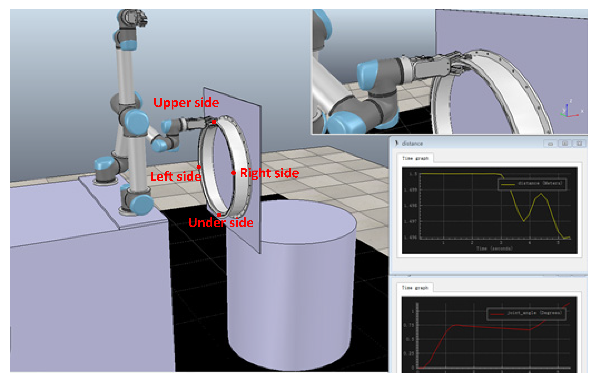
7]. We conducted a simulation analysis on the configuration change in the combined spacecraft during post-capture control, as shown in
Figure 1 and
Table 1. Details of this simulation are the same as the experimental parameters in
Section 5, and the experiment is performed under standard conditions with 1 atmosphere pressure and at 25 degrees centigrade. The space robot used a robotic arm to capture the geometric irregularities of space debris, such as the docking ring of the scrapped spacecraft. During the post-capture operation process, it can be found that the configuration of the combined spacecraft was time-varying. This time-varying configuration would cause the inertial parameters to change, making it difficult to construct the dynamics of the combined spacecraft. It further affects the success of the post-capture control. Therefore, a proper control method for all configurations is critical to achieve accurate orbital and attitude operation. Investigations of space robots have focused on the collision avoidance control of module transportation [
8,
9,
10], disturbance robust control [
11,
12] and model uncertainty adaptive control [
13,
14]. Few methodologies or design practices are in place to help engineers design with space operation in mind. For example, very little work has been carried out on the benefits and disadvantages of control system algorithms for space operation applications.
Mohan et al. [
15] proposed a dynamic control model generation method for on-orbit assembly tasks. A dynamic model was built of different stages, such as the capture, transport, and docking phases. On the basis of this, the dynamic control model generation method of the space robot was proposed. Maybeck et al. [
16] proposed the reconfigurable flight control based on the multi-model adaptive control method, which solved the control problem of the entry module of the Mars Science Laboratory. She et al. [
17] designed an adaptive controller for on-orbit service missions dependent of the model generation method. Model generation architectures were classified by the amount of a priori information by designer. Additionally, unknown parameters identification of each stage is required.
The dynamical parameters identification method is a mainstream technique for space operation, and a large number of investigations have been carried out using this method. As an example of the space robot estimation algorithms, Nguyen-Huynh et al. [
18] developed an online momentum-based estimation method for inertia parameter identification after the space manipulator grasps an unknown target. On the basis of this, an adaptive reactionless control algorithm was provided for the combined spacecraft attitude stabilization. Norman et al. [
19] provided an onboard parameter estimation scheme based on measurement equations describing the angular momentum and kinetic energy states of the rigid-body system. Mortari et al. [
20] provided an optimal linear attitude estimator algorithm of spacecraft attitude using the minimum-element attitude parameterization. According to the above investigations, the diagonal elements of spacecraft inertia matrix identification can be successfully realized. However, as reported in [
21], the takeover of a non-cooperative target can also have significant effects on the non-diagonal elements of the inertia matrix, and the effects may impart large amounts of error on the control of the combined systems. In response to this problem, Thienel et al. [
22] presented a spacecraft inertia adaptive identification method, which could estimate all spacecraft inertia components instead of only estimating the diagonal elements of the inertia matrix. Crassidis et al. [
23] made a survey of nonlinear attitude estimation methods.
The dynamic control model generation and unknown parameters identification methods can theoretically solve the control problem of space operation. However, the control precision is affected by the particle degree of the dynamic classification, and strongly related to the prior experience of the designer. In contrast to the above model-dependent control methods, Hou et al. [
24] put forward a MFC method, which can achieve convergence without a dynamics model. Bu et al. [
25] studied the stability of the MFC method in the case of data loss. Wang et al. [
26] proposed a MFC method considering external environmental disturbance, which eliminated the influence of environmental disturbance on the motion of space robots. Vikas et al. [
27] proposed a control framework of a soft robot based on the model-free theory to solve the time-varying problem of the model in the operation process. Han et al. [
28,
29] applied the model-free control (MFC) method to the post-capture combined spacecraft for the first time. In Refs. [
28,
29], researchers believed that the configuration change only caused the inertia of the combined spacecraft to change and, based on this assumption, the MFC was designed and verified. However, She et al. [
17] proposed that the relatively non-linear motion inside the combined spacecraft was the most important influence caused by the configuration change. The above investigations show that the application MFC to PCCS has not yet formed a unified cognition, and that it would benefit from further research. Compared with Refs. [
28,
29], the main contributions of this paper are as follows:
- (1)
The standardized expression form of a multiple input and multiple output (MIMO) system for the attitude and orbital dynamics of PCCS is proposed;
- (2)
An online optimization method of the data mapping model is provided to guarantee the rapid convergence of MFC;
- (3)
The test system based on the ground-based three-axis spacecraft simulator is built to verify the effectiveness of the application of the MFC method to the attitude and orbital control of PCCS.
In the development that follows, the mission scenario and problem statement were provided in
Section 2. The discrete dynamic linearization proof method of the PCCS system was derived in
Section 3. In
Section 4, the online optimization method of the data mapping model is presented for the MFC of PCCS. In
Section 5, a test system based on the ground-based three-axis spacecraft simulator was built to verify the effectiveness of application of the MFC method to the operation of PCCS. Finally, in
Section 6, concluding remarks summarize presented results.
2. Mission Scenario and Problem Statement
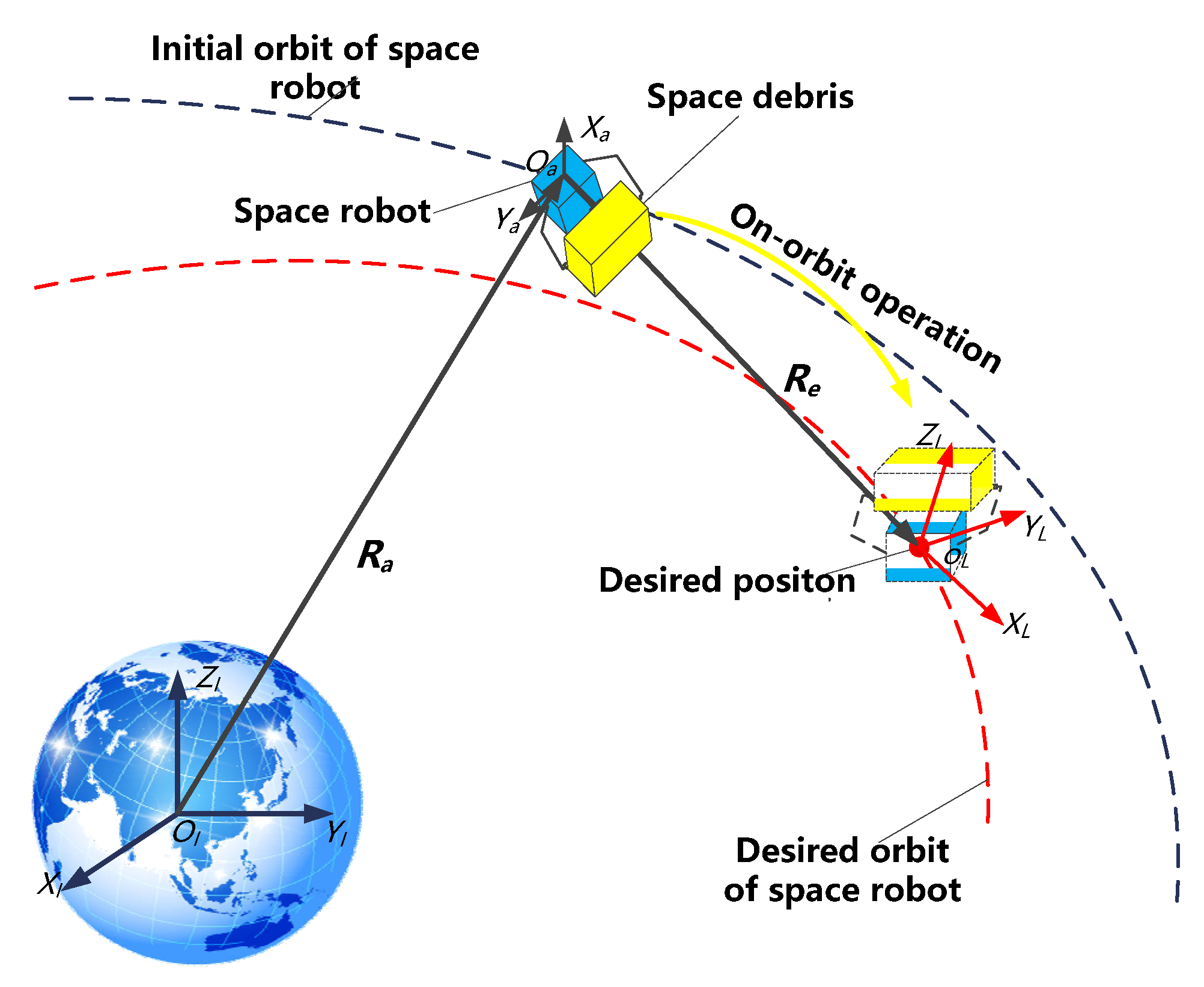
The mission scenario is designed to be an on-orbit operation of PCCS, which includes two control process, namely attitude control and orbital control.
Figure 2 depicts the mission system. Three coordinate frames are introduced in the scenario. Their definitions are given as follows.
The Earth centered inertial (ECI) frame . This frame is attached to the Earth, where axis points to the vernal equinox, axis points to the North Pole, and axis is in the equatorial plane and complies with the right-hand rule.
The body centered (BC) frame
. This frame, shown in
Figure 1, is attached to the space robot, where origin
is the combined spacecraft center, and the three axes
,
, and
are along the inertial principal axes of the space robot, respectively.
The virtual centered (VC) frame . The origin is the virtual desired point, and its axes are parallel to the inertial coordinate system.
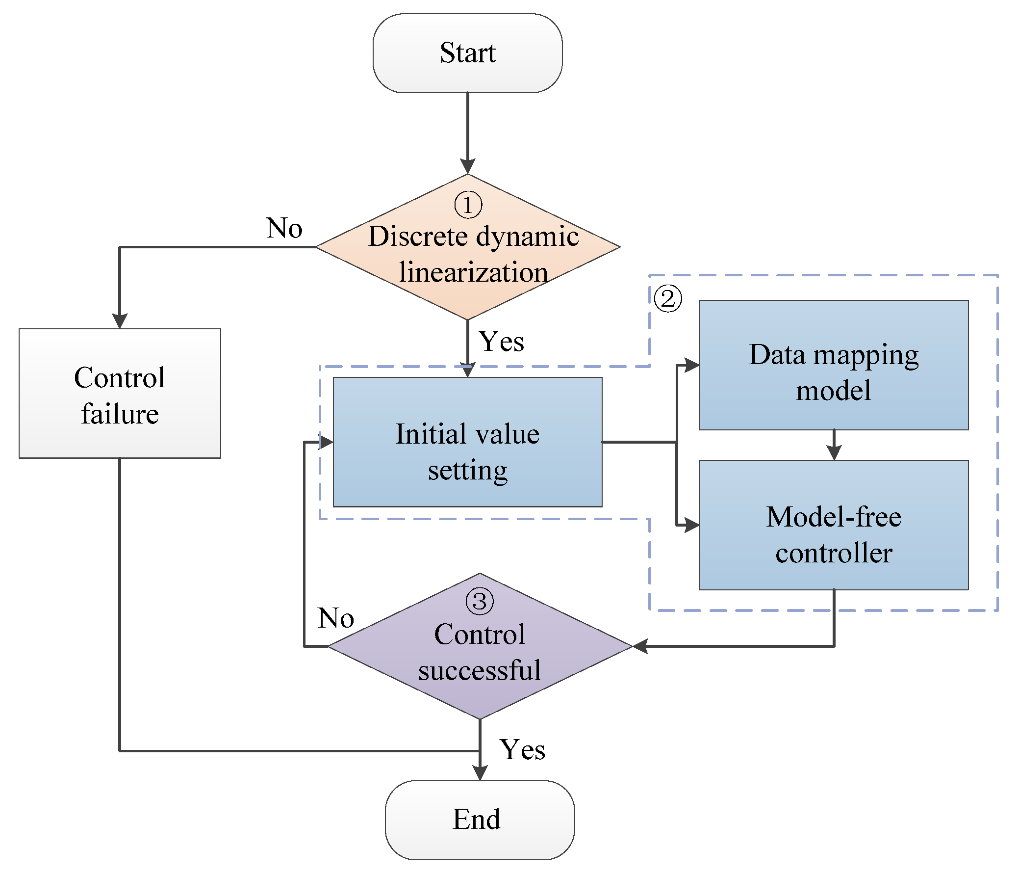
When applying MFC method to this mission scenario, further control flow was represented in
Figure 3.
It can be seen from
Figure 3 that the control process has three key links, as follows:
① Discrete dynamic linearization—based on the input and output variables, the MFC method is applicable only when the nonlinear dynamic equation of the space robot can be discretely and dynamically linearized;
② Initial values assignment of data mapping model and MFC—initial values assignment is key for the convergence of MFC, since the convergence time of the MFC method is positively related to the accuracy of the data mapping model, and the appropriate initial assignment can realize the rapid construction of the data mapping model;
③ Control effectiveness verification—the MFC method investigated in this paper was aimed at a PCCS, which had a variable configuration and time-varying dynamics. Control effectiveness was difficult to verify by the method of numerical modeling. It is necessary to construct the PCCS simulator with space–ground consistency to verify the effectiveness of control.
In response to the above three issues, the discrete dynamic linearization method of the dynamics model for PCCS was proposed in this paper. Then, an initial value online optimization method was proved. On the basis of this, a test system based on the ground-based three-axis spacecraft simulator was built to verify the effectiveness of control.
4. Online Optimization of the Data Mapping Model
As shown in Equation (16), the model-free controller is constructed by using the input data and the output . The advantage of this method is that, based on a limited number of input and output data, the MFC method can realize its control objective in real-time without pre-training. However, in Equation (16), in addition to the constant parameters , , the controller also includes the time-varying matrix . In particular, is key for the convergence characteristics of the controller. Considering that is the dynamic linear relationship matrix between input data and output data, as shown in Equation (15). In this paper, is defined as the data mapping model.
As far as the researchers know, there is no research on the optimal assignment of in MFC theory. In engineering applications, the initial value of is usually set to a very small value to ensure that the initial control input is too large to cause the combined spacecraft to lose control. However, the result of this method is that it will lead to control divergence due to external interference. In this paper, combining the discrete linearization equation of the PCCS in Chapter 3, the initial assignment of the data mapping model is optimized to ensure that the control process can converge without causing the combined spacecraft to lose control.
According to Equation (13), we can obtain the following:
Based on Equations (15) and (18), the initial value of the data mapping model can be optimized as follows:
where
is the initial value of the data mapping model
;
denotes the initial value of
;
and
denote the initial estimate of
and
, respectively.
The mass and moment of inertia of the PCCS are unknown, since the operation object is a non-cooperative target. Therefore, is an unknown value. The purpose of the following development is to propose an estimation method for .
In Equation (19),
,
, and
consist of
,
,
,
,
, and
, where
,
,
, and
is measurable. Here,
can be directly estimated using the input and output data at the first moment. Equation (20) is as follows:
When estimating
, the nonlinear influence caused by the configuration change and the external influence are ignored. Based on the Equation (4), the formula can then be developed as follows:
where
,
.
In the post-capture control task of non-cooperative targets, the matrix
is completely unknown. As mentioned in
Section 1, the traditional solution for this problem is to estimate the matrix. However, it is determined that Equation (21) is unsolvable if one considers the nine elements of matrix
as unknowns. Therefore, the previous investigations assume that the inertia matrix has a symmetric form, that is
,
,
, and the number of unknowns is reduced to six. Then, the least squares method or Kalman filter method are used to estimate the six unknown parameters. However, it is obvious that the PCCS is not a regular rigid body in actual situations, which means that the assumption that the matrix
is symmetrical does not hold. This is also an important reason why traditional dynamic parameter identification and model-based control methods are difficult to apply to PCCS operation.
The model-free controller used in this paper has the function of data model self-adaptation and does not need to obtain the precise dynamic parameters of the combination. In the actual situation, considering the actual situation, the parameters of the inertia principal axis are much larger than other parameters and, thus,
. Therefore, we only estimate the parameters of the principal axis of inertia. Then, Equation (21) can be further expressed as follows:
The initial value of the data mapping model, , was obtained though the above method. This method can provide an exact initial value of parameter , instead of the initial value given by the researcher based on experience.
5. Experimental Results
This section will apply the proposed control and optimization method to the problem of post-capture combined spacecraft attitude and orbital control, along with accompanying experimental results.
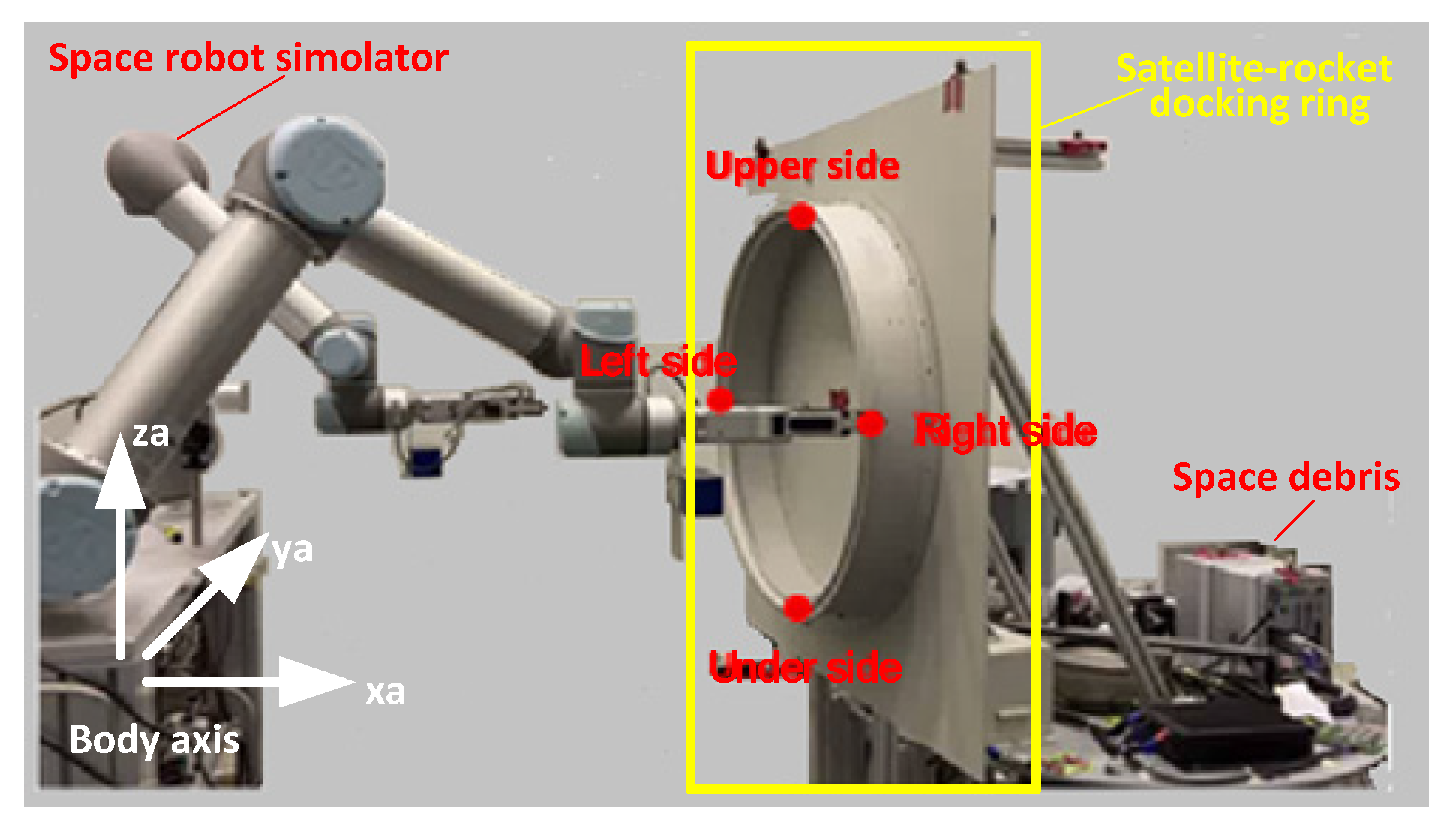
To test the proposed control and optimization method on the ground, firstly, a three-degree-of-freedom simulator of PCCS was developed.
Figure 4 shows the structure of the simulator. The space robot used two robotic arms to capture the docking ring of the space debris. The mass of the space robot and the space debris are roughly equal, at about 120 kg. The single-axis attitude freedom of the simulator is actuated by a flywheel. The theoretical maximum torque of the flywheel is 0.1 N·m, and the maximum speed is 6000 revolutions per second. The two-axis position freedom of the simulator is actuated by eight sets of thrusters. The theoretical maximum force of the thrusters is 0.1 N. The control torque of the flywheel and the control force of thrusters (the input data of PCCS) are transferred to the control computer through the RS232 serial port. The position data and attitude date (the output data of PCCS) are measured by eight cameras and transferred to the control computer through the RS232 serial port. The sampling period is 0.1 s. In the experimental system, a personal computer was used as the control computer to develop the control program by using Simulink software. During the control process, the configuration of the simulator changes with time.
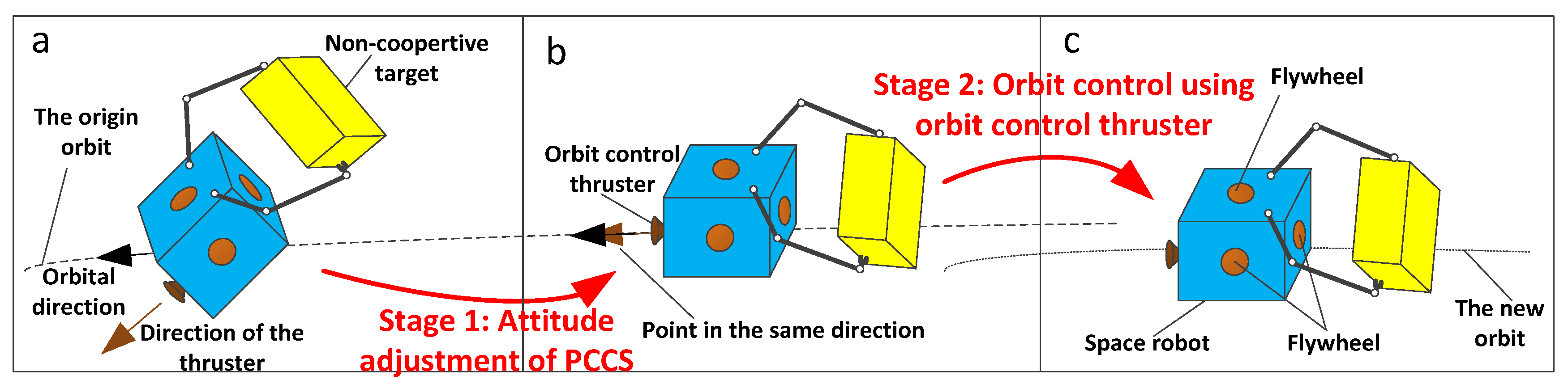
To test the proposed control and optimization method on the ground, secondly, an orbit change task was designed. In this task, the space debris was dragged off the origin orbit to a new orbit.
Figure 5 shows the flow of this task. As shown in
Figure 5, this task was divided into two stages. The first stage is the attitude adjustment of PCCS. The purpose of this stage was to adjust the attitude of the combined spacecraft and to provide a feasible attitude condition for the orbit change in PCCS. The second stage is the orbit control of PCCS and, in this step, the combined spacecraft maneuvered into a new orbit by using its orbit control thruster. Orbit change is a common method for space debris removal missions to free up precious orbital resources occupied by space debris. In the experiment, two cases were designed to simulate the two stages of orbit change task, namely attitude maneuver control and position maneuver control.
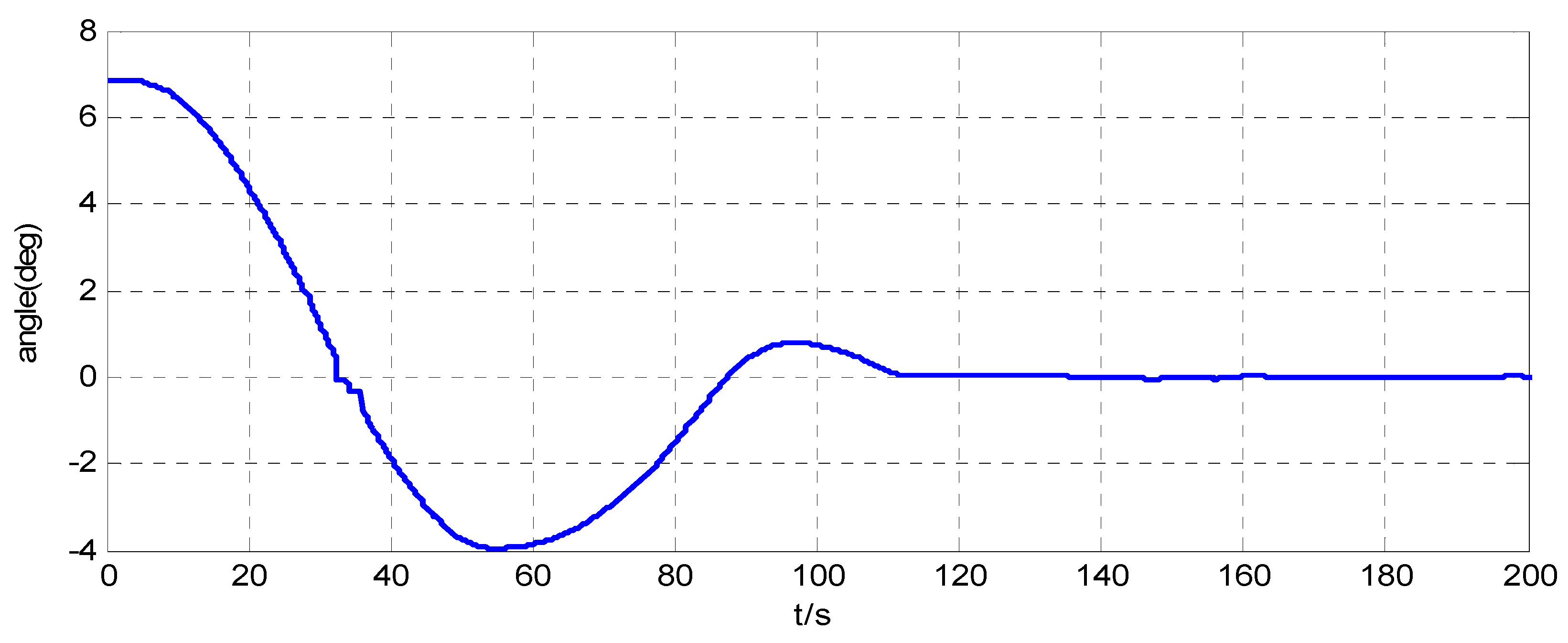
Case 1. Attitude maneuver control
In this case, two groups of tests are provided. In the first group of tests, the initial angle and angular velocity of the simulator are
and
, respectively. The desired angle and angular velocity of the simulator are set to
and
, respectively. The parameters of controller
,
,
,
, and these parameters are defined in Equations (16) and (17). In addition, based on the three-degree-of-freedom simulator of PCCS shown in
Figure 4, the attitude maneuver control around the z-axis was realized by using the flywheel installed on the space robot simulator. The tests results are shown as
Figure 6,
Figure 7,
Figure 8 and
Figure 9.
In the second group of tests, the initial angle and angular velocity of the simulator are
and
, respectively. The desired angle and angular velocity of the simulator and parameters of the controller are the same as that of the first group of tests. The tests results are shown as
Figure 10,
Figure 11,
Figure 12 and
Figure 13.
Case 2. Position maneuver control
In this case, two groups of tests are provided. In the first group of tests, the initial position and velocity of the simulator are
and
, respectively. The desired position and velocity of the simulator are set to
and
, respectively. The parameters of controller
,
,
,
, and these parameters are defined in Equations (16) and (17). The position maneuver control along the x-axis was realized by using the thruster installed on the space robot simulator. Test results are shown as
Figure 14,
Figure 15,
Figure 16 and
Figure 17.
In the second group of tests, the initial position and velocity of the simulator are
and
, respectively. The desired position and velocity of the simulator are set to
and
, respectively. The parameters of the controller are the same as those of the first group of tests. Test results are shown as
Figure 18,
Figure 19,
Figure 20 and
Figure 21.
The attitude maneuver control experimental results are shown in
Figure 6,
Figure 7,
Figure 8,
Figure 9 and
Figure 10.
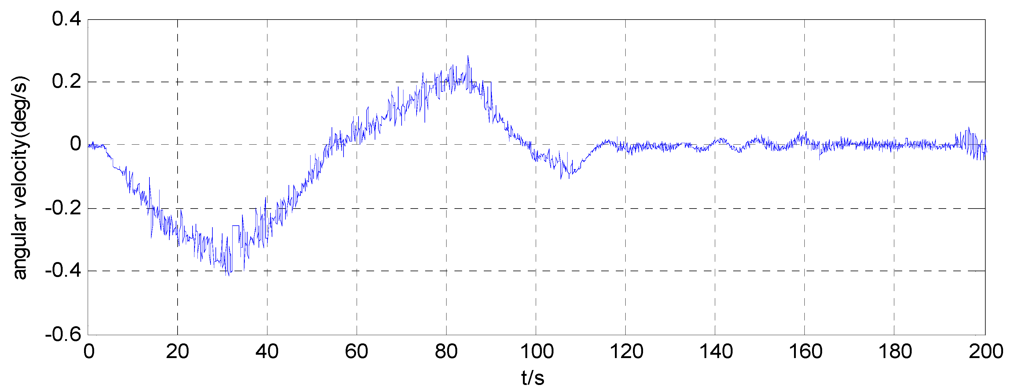
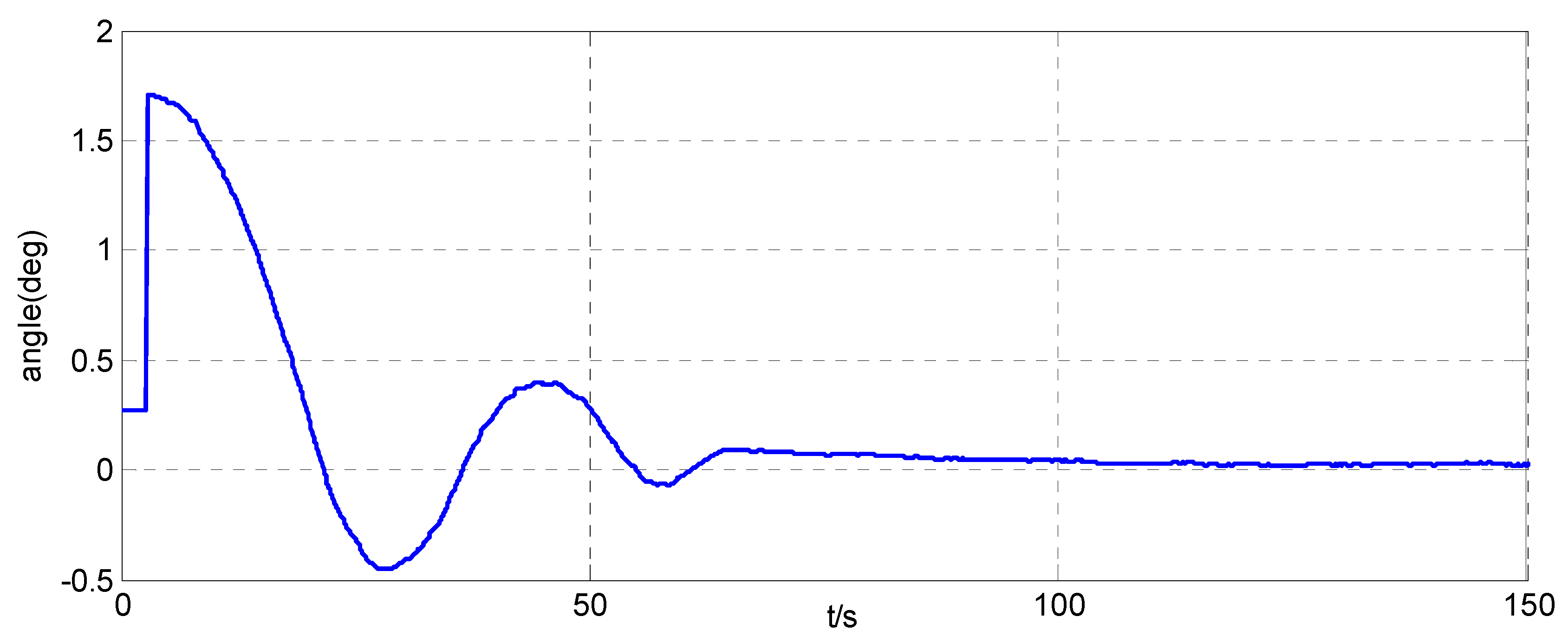
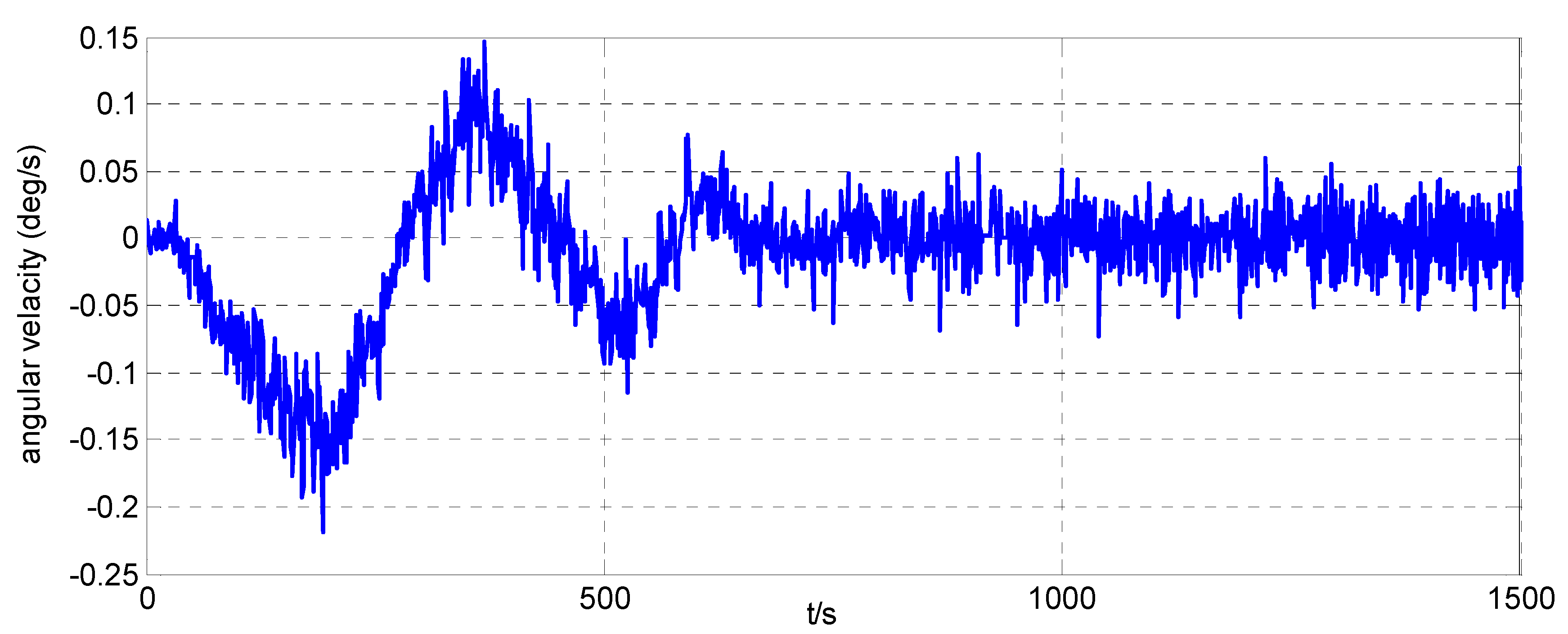
Figure 6 and
Figure 10, and
Figure 7 and
Figure 11, are the angle curve and angular velocity curve of the simulator, respectively.
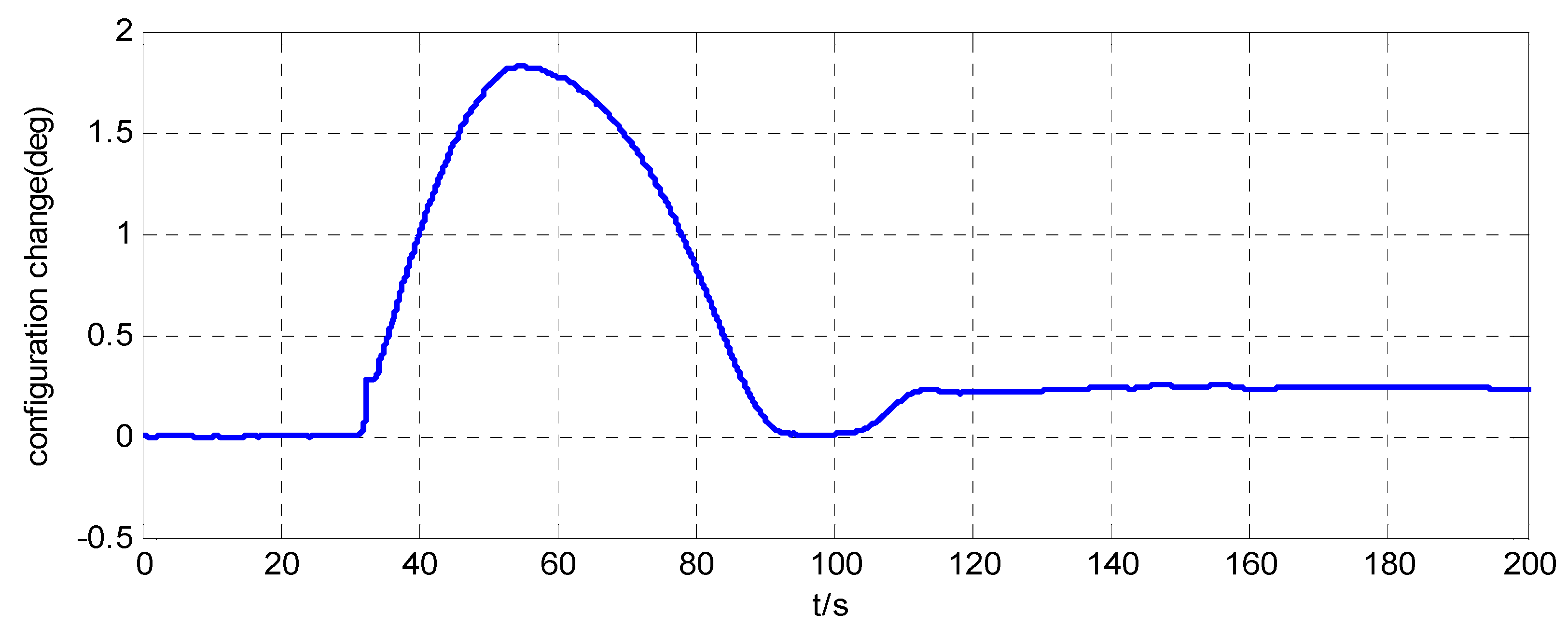
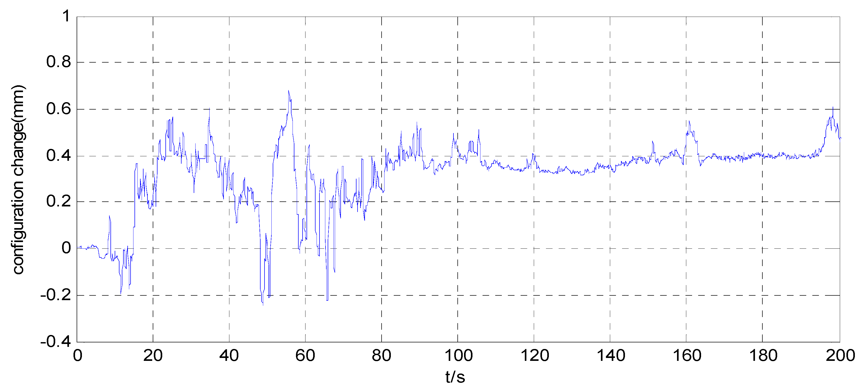
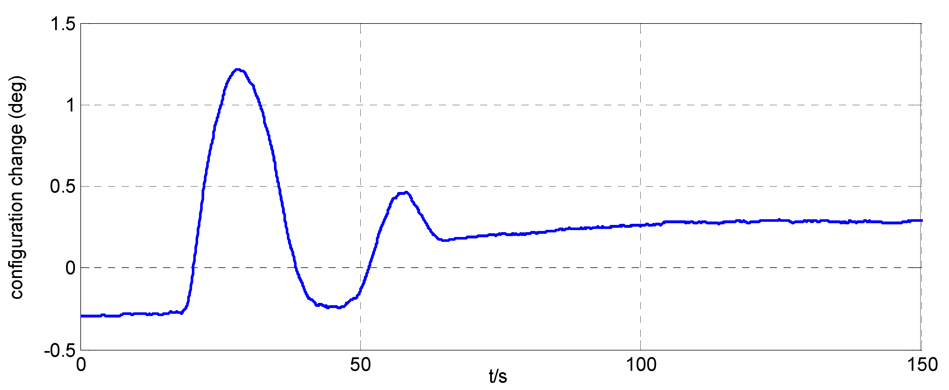
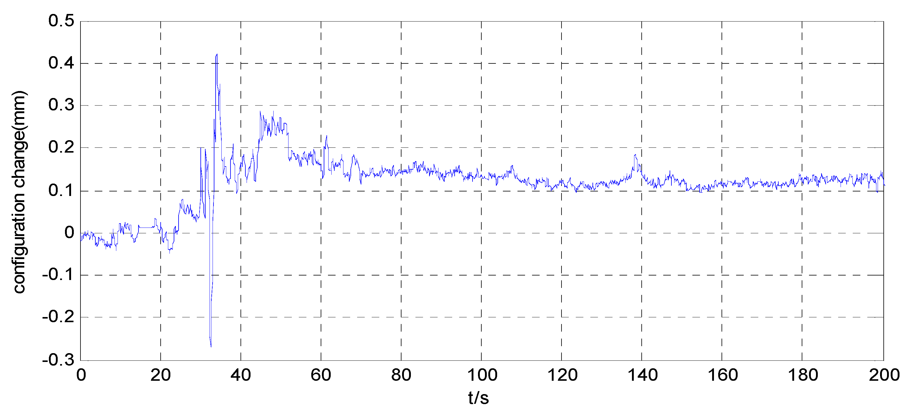
Figure 8,
Figure 9,
Figure 12 and
Figure 13, show the configuration change inside the combined spacecraft during the attitude maneuver. From
Figure 6,
Figure 7,
Figure 10 and
Figure 11, it can be observed that the angle and angular velocity of the simulator converge to the desired states asymptotically. The attitude configuration change can reach nearly
during the control process, as shown in
Figure 8 and
Figure 12. Compared with attitude configuration, the position configuration change in the simulator is relatively small, at about 1 mm, as shown in
Figure 9 and
Figure 13. In the case of the above configuration changes, the attitude control of the spacecraft still achieves very high accuracy by using the MFC method, as shown in
Figure 6,
Figure 7,
Figure 10 and
Figure 11. In addition, we adjusted the initial angle of the simulator and carried out several groups of tests. The test results show that model-free control algorithm can also achieve a good control effect, if the energy of the actuator is sufficient. That is, the control effect is independent of the initial state of the system.
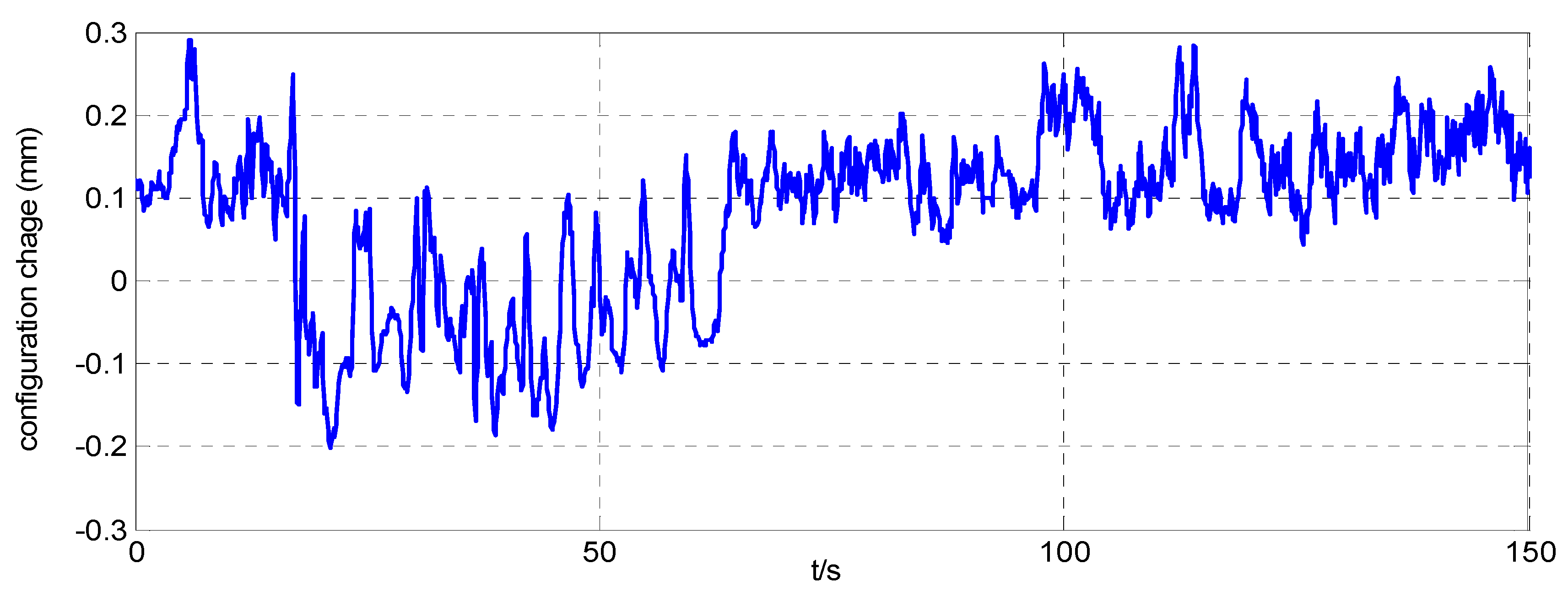
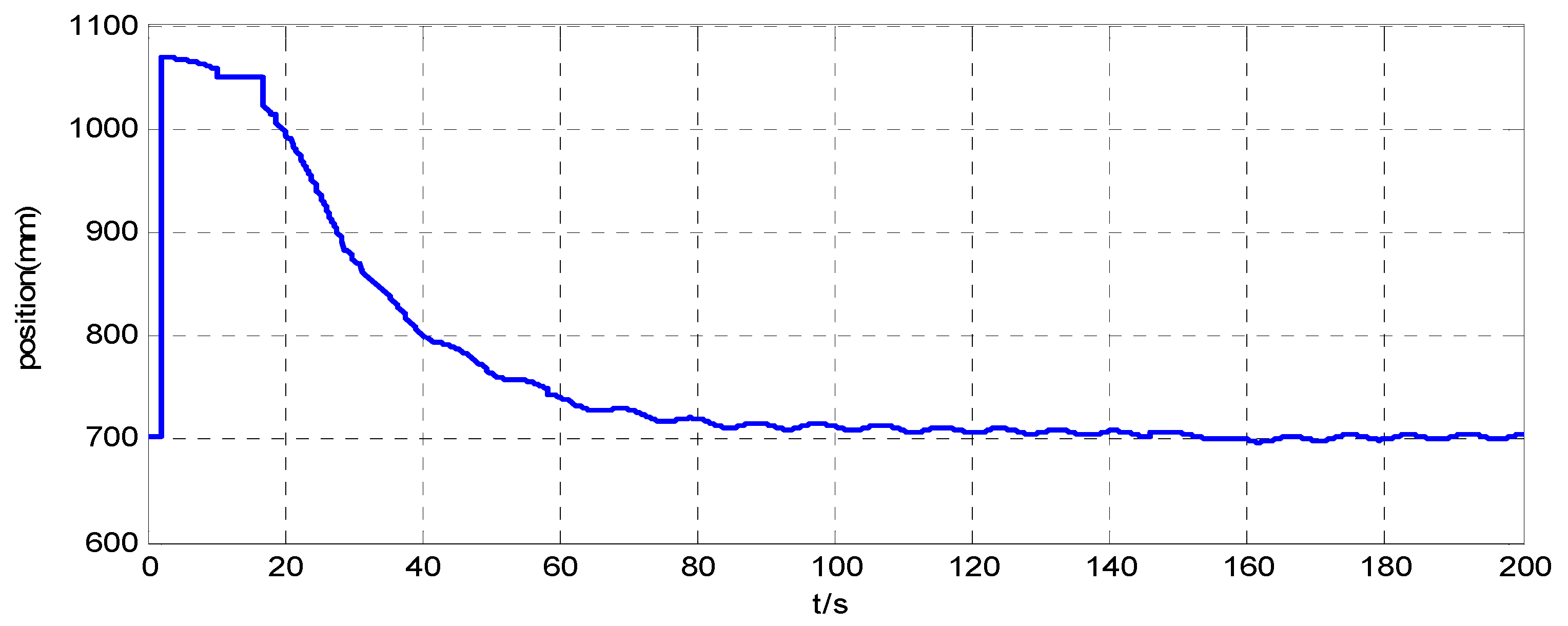
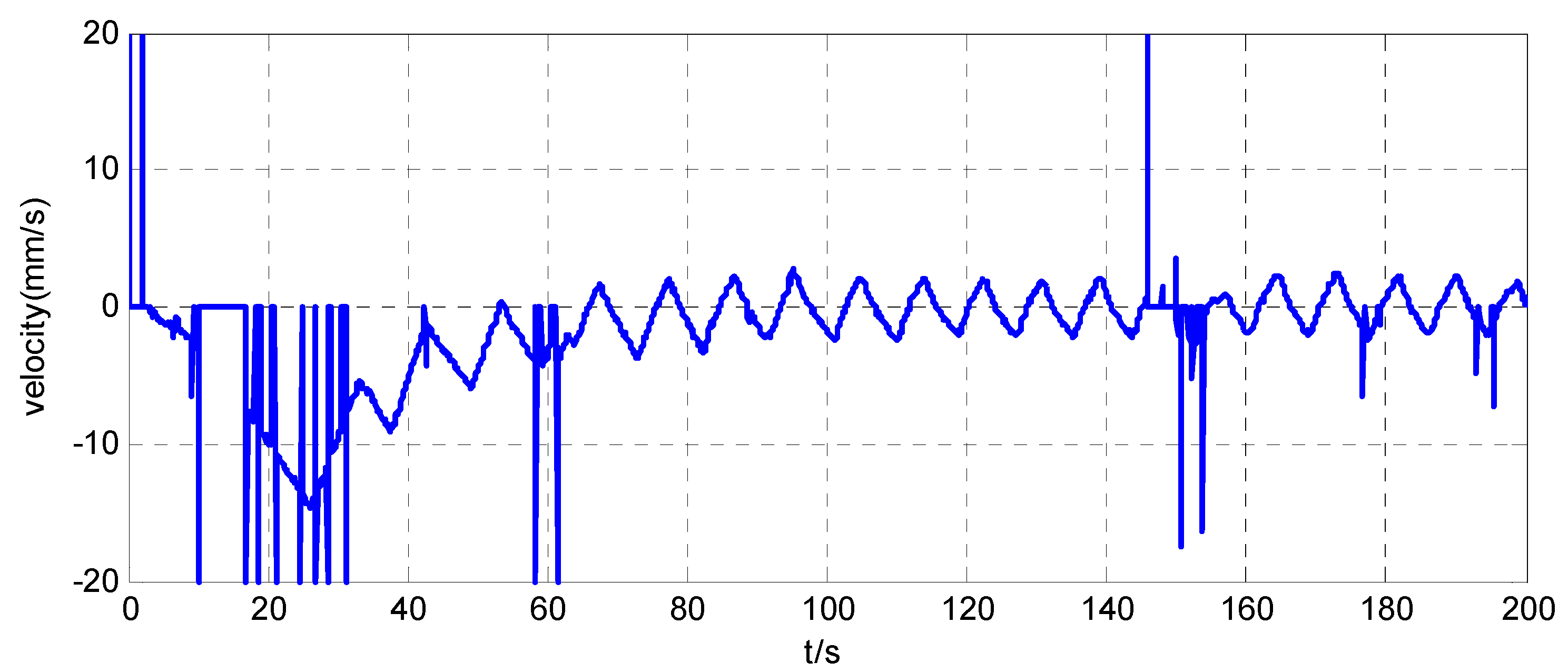
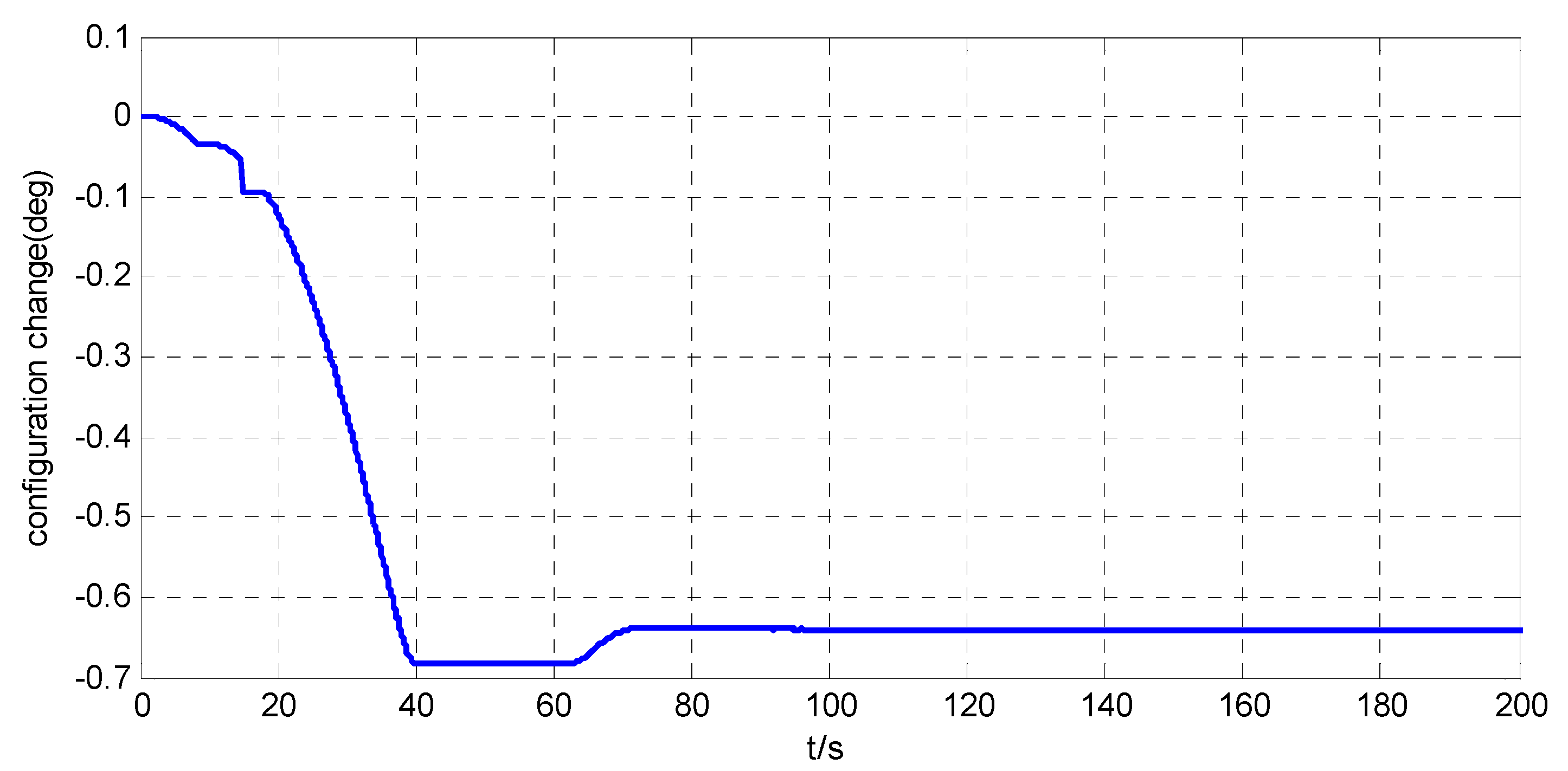
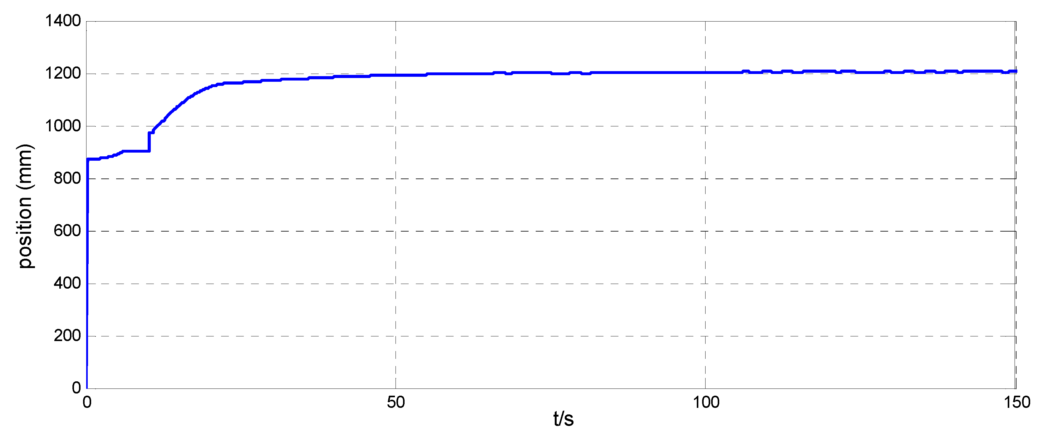
The position maneuver control experimental results are shown in
Figure 14,
Figure 15,
Figure 16,
Figure 17,
Figure 18,
Figure 19,
Figure 20 and
Figure 21.
Figure 14 and
Figure 18, and
Figure 15 and
Figure 19, show the position curve and velocity curve of the simulator, respectively.
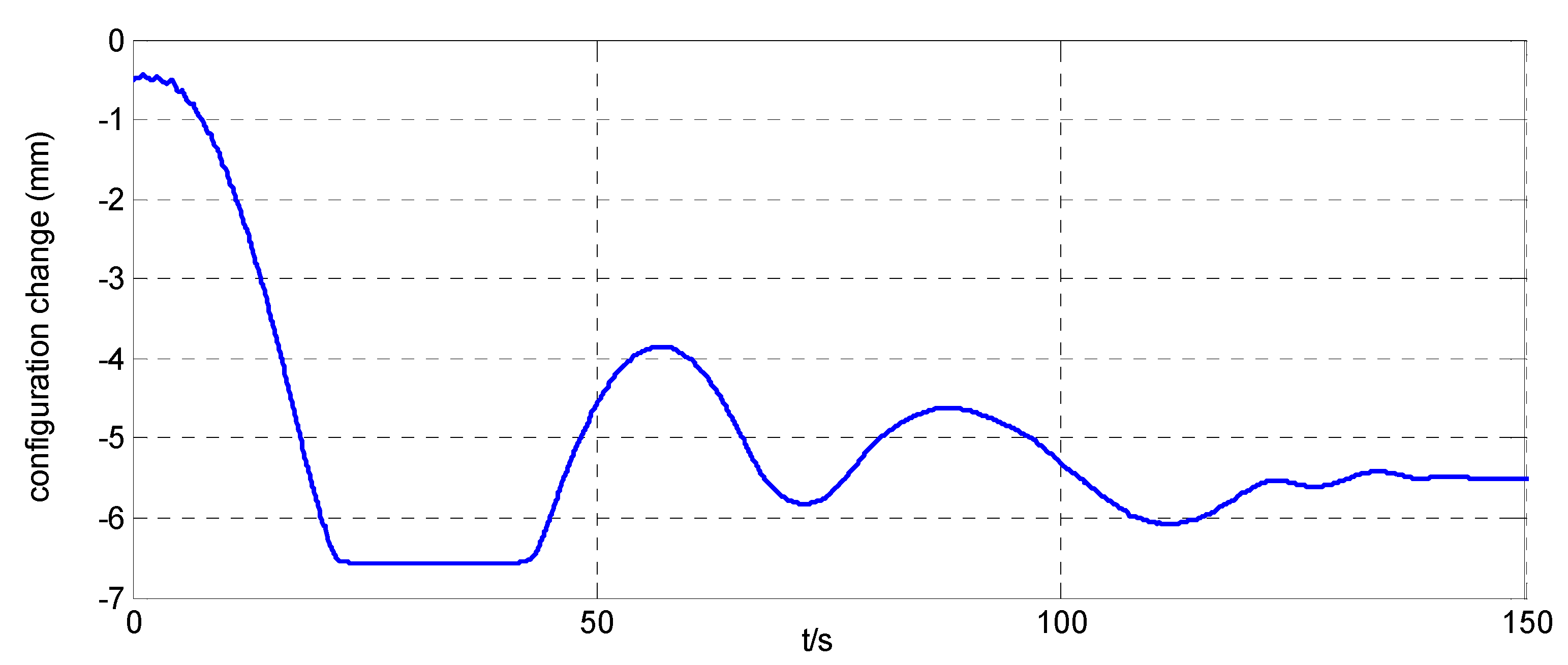
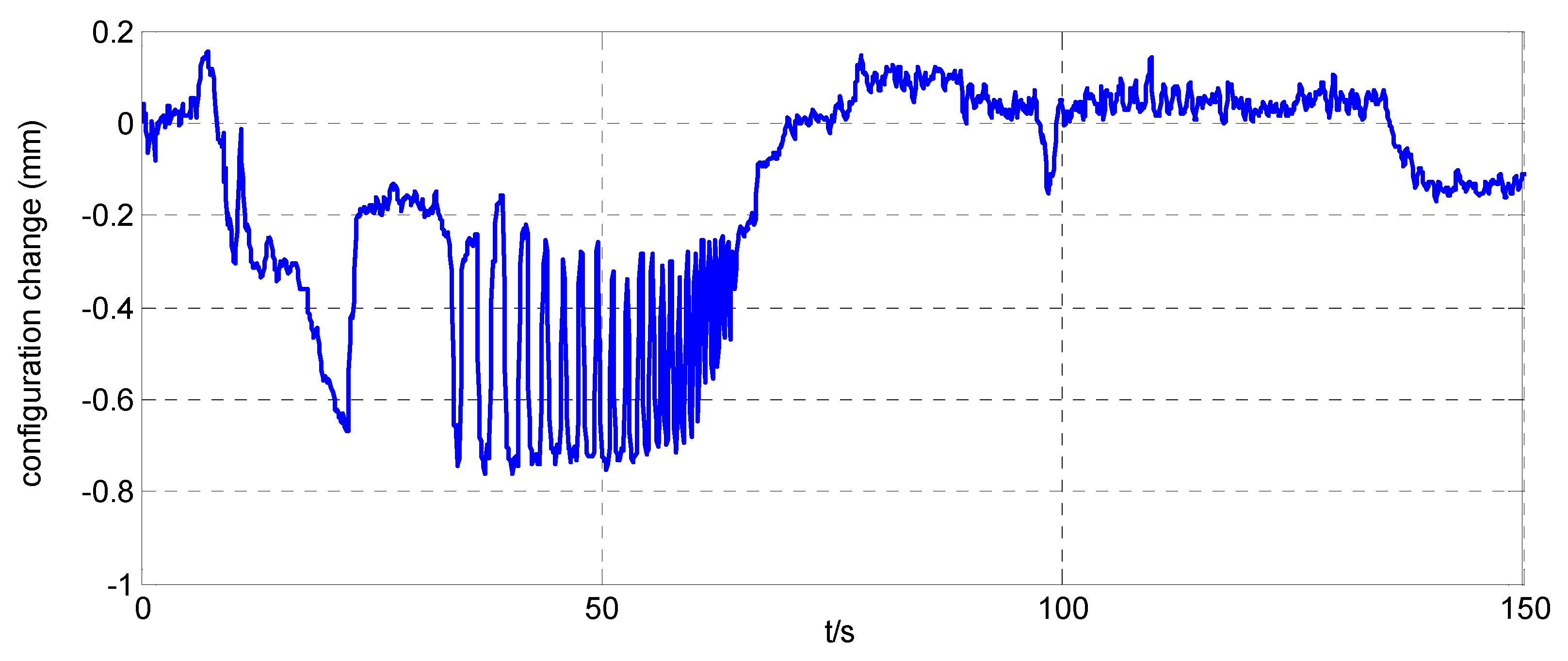
Figure 16,
Figure 17,
Figure 20 and
Figure 21, show the configuration change inside the combined spacecraft during the position maneuver. As shown in
Figure 14,
Figure 15,
Figure 18 and
Figure 19, the position control of combined spacecraft is achieved by using the control and optimization method proposed in this paper, in the case of measurement errors in individual data. Furthermore, during the position maneuver control, the simulator has a configuration change. The maximum angle configuration change can reach nearly
. From the above experimental results, the effectiveness of the application of the MFC and optimization method to the operation of PCCS is proved.
According to the ground test results, the advantage of MFC in spacecraft attitude and orbit control is its fault tolerance. That is, even if the measured data is distorted at a certain time, the control curve is still smooth and good control effect can be achieved finally. In contrast, the weaknesses of MFC is that it has many parameters, which makes it difficult to achieve a good control effect. As shown in
Figure 6 and
Figure 10, the attitude curve has overshoot, and this is a result of non-optimal parameter selection. To solve this problem, our next work is to design an adaptive parameter adjustment algorithm to achieve the optimal control effect of MFC.


