Article

High-Accuracy Finite Element Model Updating a Framed Structure Based on Response Surface Method and Partition Modification

1
School of Mechanical Engineering, Dalian University of Technology, Dalian 116024, China
2
State Key Laboratory of Robotics, Shenyang Institute of Automation, Chinese Academy of Sciences, Shenyang 110169, China
3
School of Mechanical Engineering & Automation, Northeastern University, Shenyang 110819, China
*
Author to whom correspondence should be addressed.
Aerospace 2023, 10(1), 79; https://doi.org/10.3390/aerospace10010079
Submission received: 23 October 2022 / Revised: 11 January 2023 / Accepted: 12 January 2023 / Published: 13 January 2023

Abstract

:
In this paper, a finite element model updating (FEMU) method is proposed based on the response surface model (RSM) and genetic algorithm (GA) to establish a high-precision finite element (FE) model of space station scientific experiment racks. First, the fine solid and mixed FE models are established, respectively, and a comparison of the modal test results is conducted. Then, an orthogonal experimental design is used to analyze the significance of the parameters, and the variables to be modified are determined. The design parameters are sampled via the Latin hyperbolic method and are substituted into the FE model to obtain the modal parameters of the scientific experiment rack. The mapping relationship between the design and modal parameters is fitted by constructing the Kriging function, and the RSM is established. The design parameters of the scientific experiment rack are optimized via GA, and the initial FE model is updated, which has the advantage of improving the computing efficiency. Finally, the updated FE model of the experiment rack is verified by frequency sweep and random vibration tests. The experimental results show that the proposed approach has high precision and computing efficiency, and compared with the test results, the modal frequency errors of the updated model are within 5%, and the vibration response errors under random excitation of the updated model are within 7%.

1. Introduction

The framed structure with a combined form made of beams and skin has been widely used in engineering equipment, and its dynamic characteristics are significant performance indicators, especially in aerospace fields, including in scientific experiment racks on space stations. The scientific experiment rack has lots of requirements in terms of its dynamic characteristics, including a lightweight design, anti-vibration and shock-resistance capabilities during the launch phase, long-term use stability, and low vibration in orbit [1,2,3,4]. To realize the effective dynamics analysis and reasonable vibration control of the framed structures, a high-accuracy finite element (FE) model is urgently needed. At present, the most effective and reliable method is to build and update the FE model based on the manufactured structure to obtain a high-accuracy dynamic simulation model. In this paper, by taking the space station scientific experiment rack as a typical framed structure, the research on the FE modeling approach and updating method of a high-accuracy FE model is proposed, which can provide the basis for the vibration response forecasting of framed structures under complex load and excitation conditions.
Lots of work has been carried out on the FE modeling of complicated framed structures, mainly involving the processing approach used on beam and plate combinations and connection types. Aiming at studying the bolted joints in framed structures combined with beams and plates, the Sandia National Laboratory and the University of Illinois Laboratory simulated the nonlinear dynamic behaviors of framed structures considering the nonlinear stiffness and damping characteristics of bolted joints both experimentally and numerically [5,6]. Zang et al. [7] took a three-layer framed structure with bolted joints as the object and established three types of models, a solid FE model, a plate-beam FE model, and a 3-DOFs lumped mass model. The modal calculation results of the three FE models were compared with the experimental results. Then, the influence of uncertain factors, such as the bolted connection complexity, machining and assembly errors, and inaccuracy of the material parameters on the FE modeling were also discussed, and reasonable updating parameters were determined. Chang et al. [8] utilized a hybrid model combined with solid and truss elements to study the long-term effects of bridge creep. Sliseris et al. [9] proposed a multi-scale FEM for beams and frames with complex topological structures, in which the beam elements were used for coarse scales, and the continuous elements were used for fine scales. Compared with the full-scale continuum model, the multi-scale FEM can obtain the displacement, shear deformation, and local stress–strain gradients of the framed structures.
In FEMU approach research, the direct correction method and parameter modification method are commonly used. The direct correction method directly modifies the mass matrix and the stiffness matrix of the FE model. In [10], a new FEMU problem was formulated as an optimal matrix approximation problem with a significant physical meaning. The results of the numerical examples of structural dynamics show that the proposed optimal matrix method works well. Friswell et al. [11] extended the direct matrix correction method to simultaneously modify the stiffness matrix and damping matrix, which were verified by a cantilever beam. Compared with the direct correction method, the physical meaning of the parameter modification method is more clear. For example, Fox et al. [12] presented the first-order sensitivity expressions of linear structures by differentiating the characteristic equation to modify the model. Friswell et al. [13] demonstrated the effectiveness of parameterizing the modes at the element level and used the beam offset geometric and element modal parameters to modify the mechanical joints and boundary conditions. In [14], a fuzzy updating method was proposed to consider the uncertainty of the measured modal parameters, and it was verified by updating the FE model of a practical bridge with the measured modal parameters. In [15], a two-stage Bayesian FEMU procedure was presented for the prior estimation of measured modal parameters. It was shown that the proposed methodology could identify the FE model parameters with a high level of accuracy.
Recently, the sensitivity analysis method (SAM) and RSM based on the finite element were developed. The FEMU method based on the sensitivity method needs to perform a step-by-step iterative calculation, and the FE model with modified parameters is recalculated after each iteration, which usually requires a large number of calculations [16]. Mottershead et al. [17] gave a detailed sensitivity-based FEMU tutorial, applying sensitivity results to evaluate the effects of the parameters that needed to be corrected on the output. Cao et al. [18] proposed a nonlinear sensitivity-based FEMU method considering the local nonlinearity of the structure. Taking a cantilever beam with multiple nonlinear supports as a research object, the effect of the initial parameters on the performance of the proposed method was analyzed. The results showed that the proposed method could effectively update the nonlinear FE model, even in the presence of interfered measurement data and different initial parameters in the FE model. Izham et al. [19] used framed structures with bolted joints as the research object; the obtained modal parameters were the natural frequency, mode shape, and damping ratio through finite element analysis (FEA) and experimental modal analysis (EMA), and they determined selected parameters using a sensitivity analysis to update the framed FE model, thereby reducing the natural frequency difference between the FEA and EMA. The RSM refers to fitting the complex implicit relationship between the structural feature quantities and the parameters via building an explicit response surface function and establishing a surrogate model to replace the FE model to optimize the iteration process. The RSM calculation efficiency was significantly improved. Umar [20] proposed a model-updating method by combining the improved particle swarm optimization (PSO) and RSM to update the bridge model with thirteen variables, and an accurate FEM was obtained. Based on the response surface updating model and element modal strain energy (EMSE) damage index, the effectiveness of the proposed damage identification method for four simply supported steel beams through tests was verified by Niu et al. [21]. The results show that the proposed method has great potential for damage identification in real framed structures.
In this paper, an experiment rack simulator is manufactured, and an investigation of high-precision FE modeling, the FEMU method, and experimental verification are systematically performed. First, the fine solid FEM and mixed FEM of an experiment rack simulator are established, respectively. A modal correlation analysis between the calculation results and experiment results is conducted. Then, the significance analysis method is applied to select sensitive the design variables of an experiment rack simulator, and four selected design variables are sampled via the Latin hypercube method, which are inputted to calculate the modal parameters. Based on the above calculation results, the Kriging function method is used to establish the response surface model. The design parameters are optimized by GA to modify the established FE model. Finally, the updated model is verified by multi-condition tests, such as frequency sweep and random vibration tests.

2. FEMs and Modal Analysis of Experiment Rack Simulator

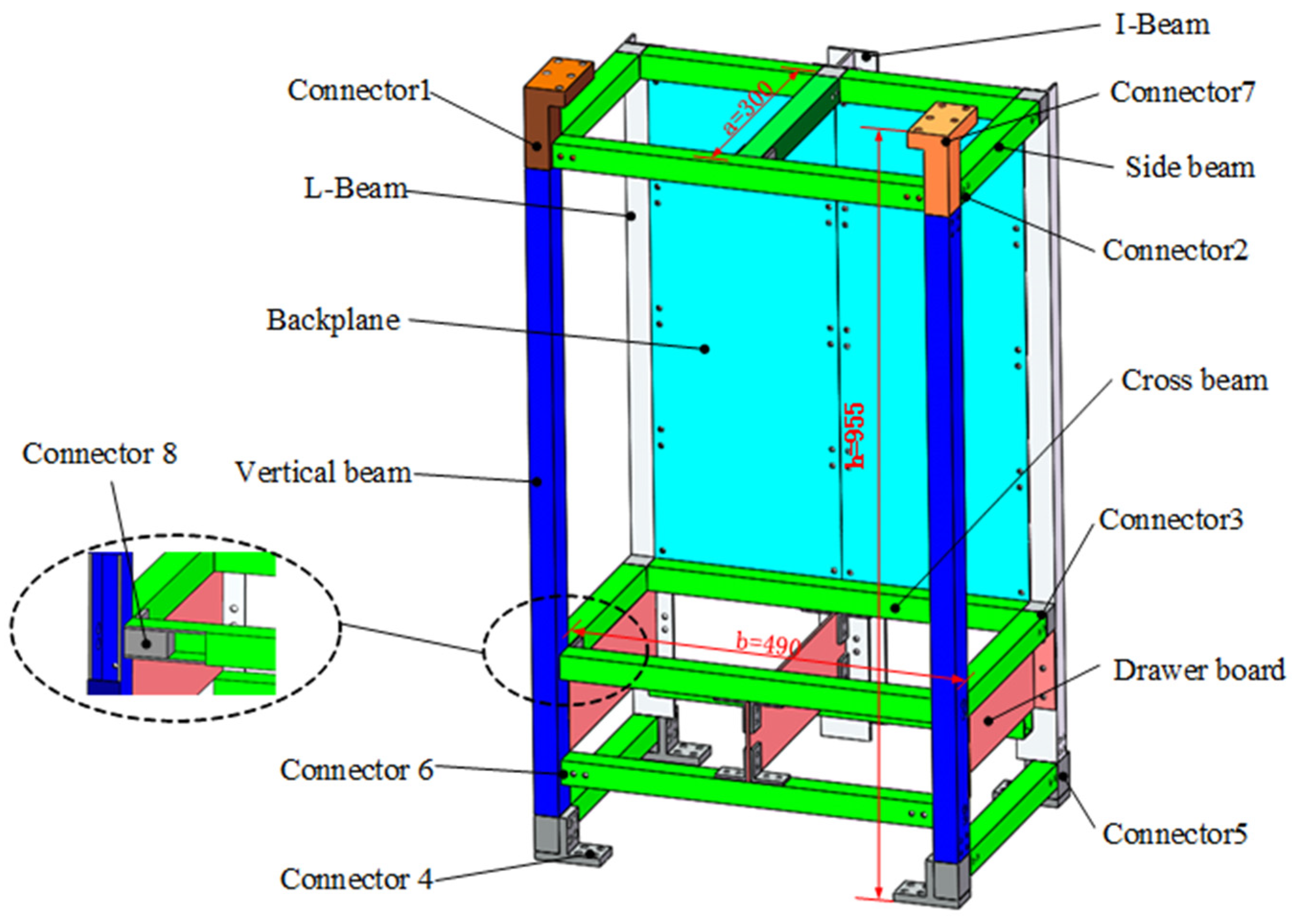
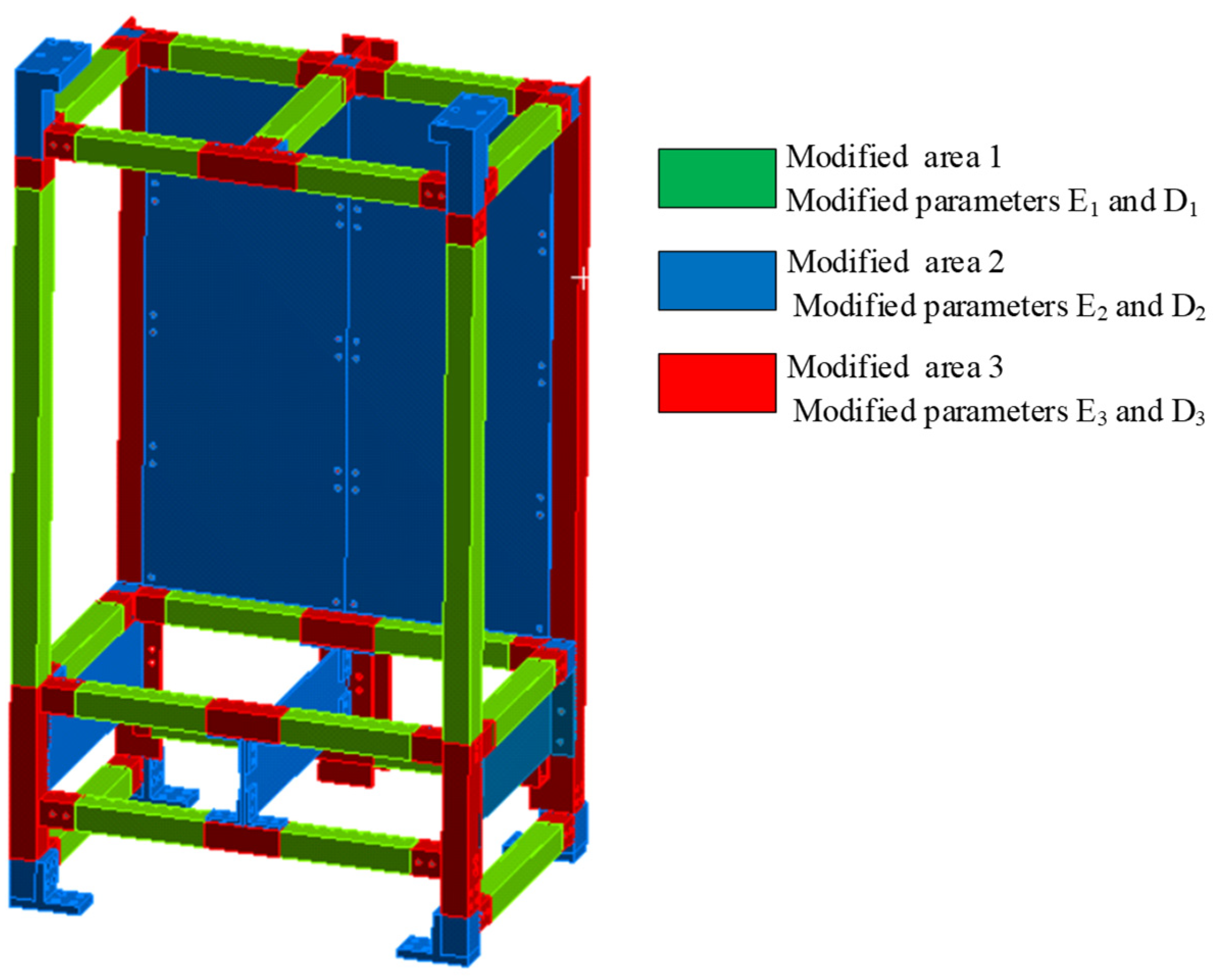
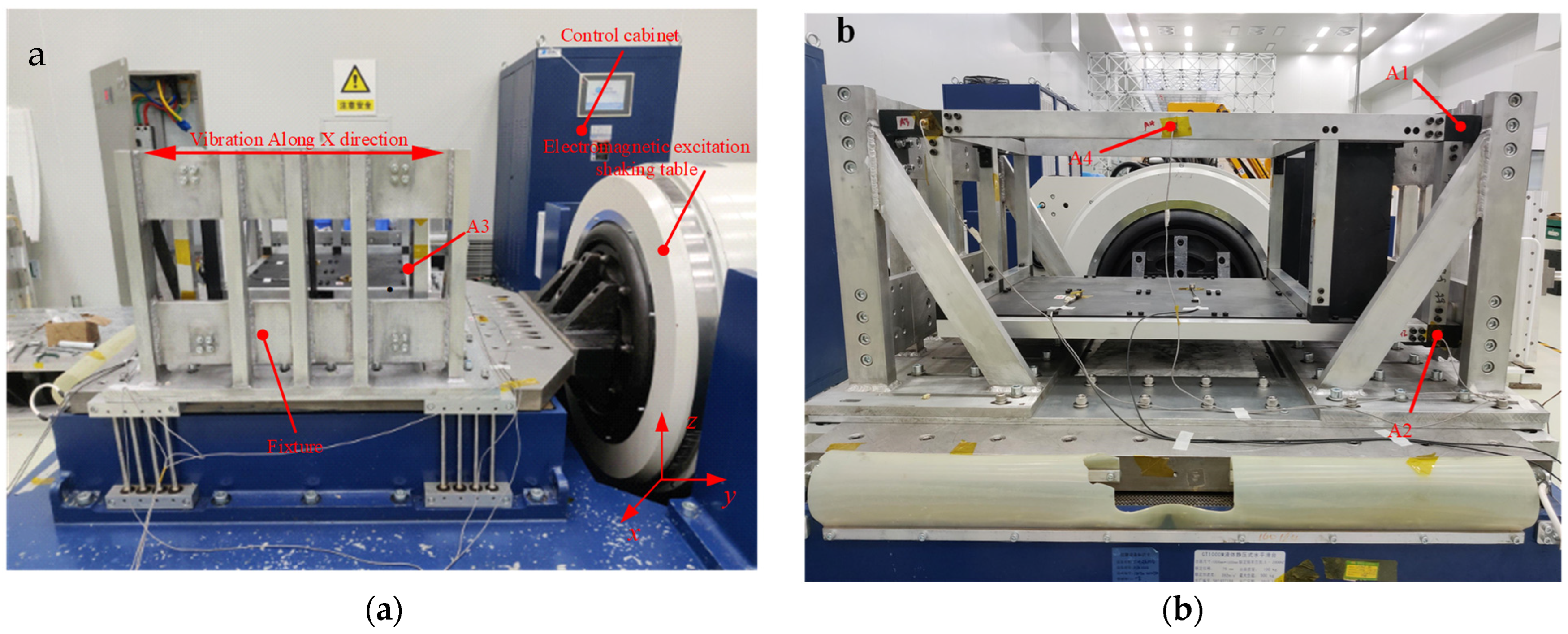
2.1. Structure Description

A space station scientific experiment rack simulator is depicted in Figure 1, which is a typical framed structure. It mainly comprises the beams, side beams, vertical beams, L-beams, I-beams, backplanes, drawer boards, connectors, and screws. The beam structure and connector are connected together by screws, the backplanes are fixed to L-beams and I-beams by screws, and the drawer boards are fixed to vertical and L-shaped beams by screws. The backplanes and side planes are the main load-bearing components.

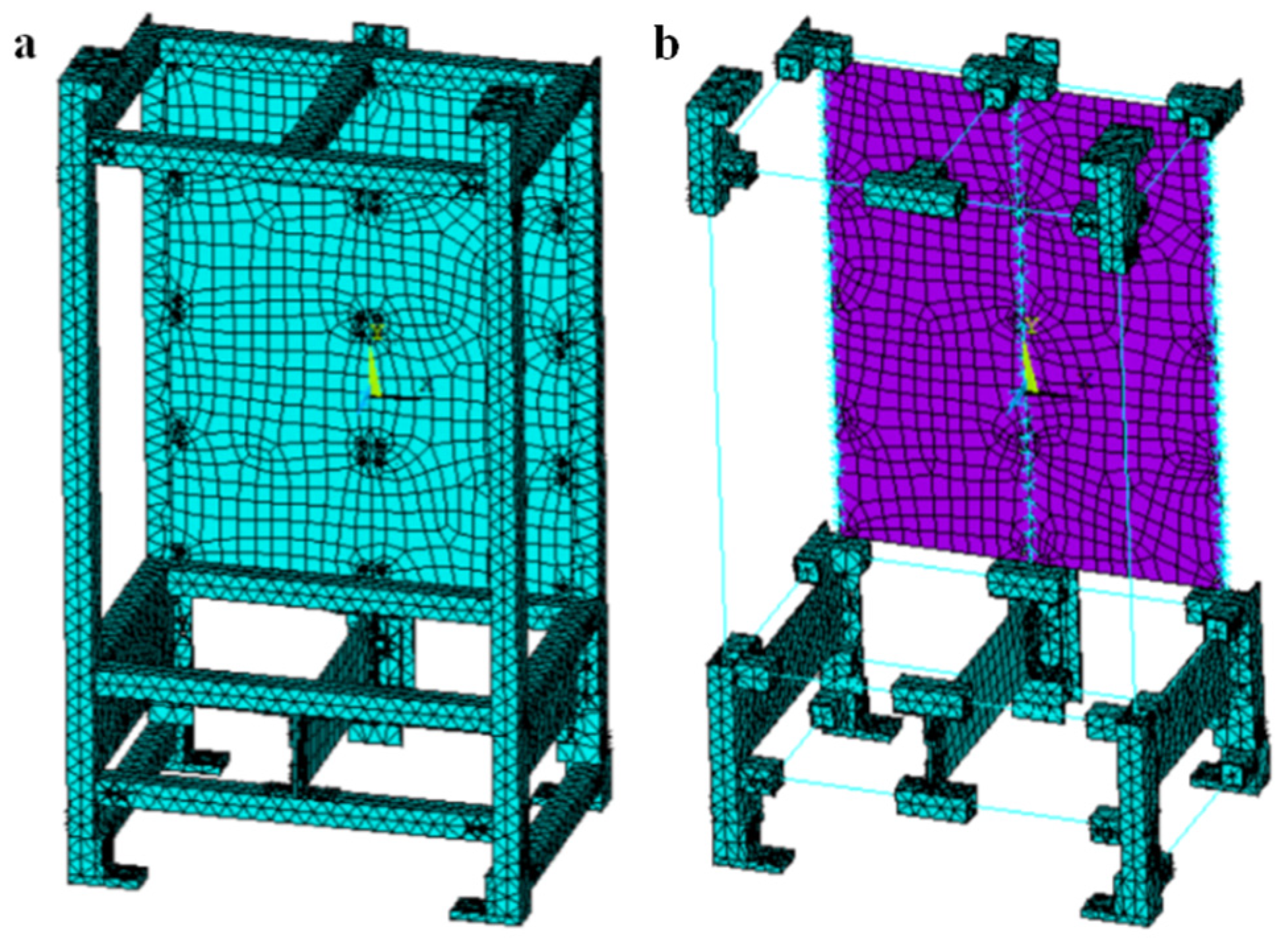
2.2. Two Types of FE Models

The experiment rack simulator is modeled with many different element types, including the beam elements, shell elements, and solid elements, based on the commercial finite element analysis (FEA) software ANSYS. The elements of FE simulation are ordered from macroscopic to microscopic: the beam element, plate element, and solid element. In actual engineering, if we start working at a large scale, a beam element or plate element can be chosen as the macro element so that the analysis time is short and the efficiency is high, but the local accurate stress distribution cannot be obtained. If we start working at a small scale, a solid element can be chosen as a micro-unit so that the accuracy of the analysis result is high, but the modeling analysis takes a long time [22]. Mixed elements modeling techniques can avoid the drawbacks mentioned above; that is, the key parts are modeled with micro-elements, the other parts are built with macro-elements, and the multiple point constraint (MPC) method is used to realize the connection between the macro-elements and micro-elements. In this section, the solid FE model and mixed FE model of the experiment rack simulator are established, respectively, and the two FE models are further modified.
Since the experiment rack simulator model contains more than 200 screws, it is not easily used for FE modeling when complex dynamic characteristics such as friction, contact, and the tightening of the screw connections are considered. Hence, the screws are simplified to be beam elements. A beam element has a circular section, and the radius and length are the same as they are in an actual screw. Since the connection between the connector and beam is an interference fit, the contact between the connector and beam is set as non-separating contact, with tangential displacement being allowed and normal displacement not being allowed.
For the solid FE model depicted in Figure 2a, the experiment rack simulator is modeled with solid186 elements, except for the screws. The material attributes of all of the beam structures are 6063 Aluminum, and those of the backplanes, drawer boards, and connectors are Q235 steel. For the mixed FE model of the experiment rack simulator depicted in Figure 2b, the solid186 element is used to model the connectors, the shell181 element is used to model the backplanes and drawer boards, and the plate thickness is set to 4 mm constantly. The rest of them are modeled using beam188 elements, and the beam section shape is controlled by real constants, including rectangular beams, square beams, L-beams, and I-beams. The MPC method connects the different elements, and the constraints between the beam endpoints and solid joint surface nodes are built. The element types, material attributes, and the number of elements and nodes of the two experiment rack simulator FE models are listed in Table 1. The number of nodes and elements contained in the solid FE model of the experiment rack simulator is 2.3 times that of the mixed FE model. Therefore, the mixed FE model of the experimental rack simulator has a higher calculation efficiency.

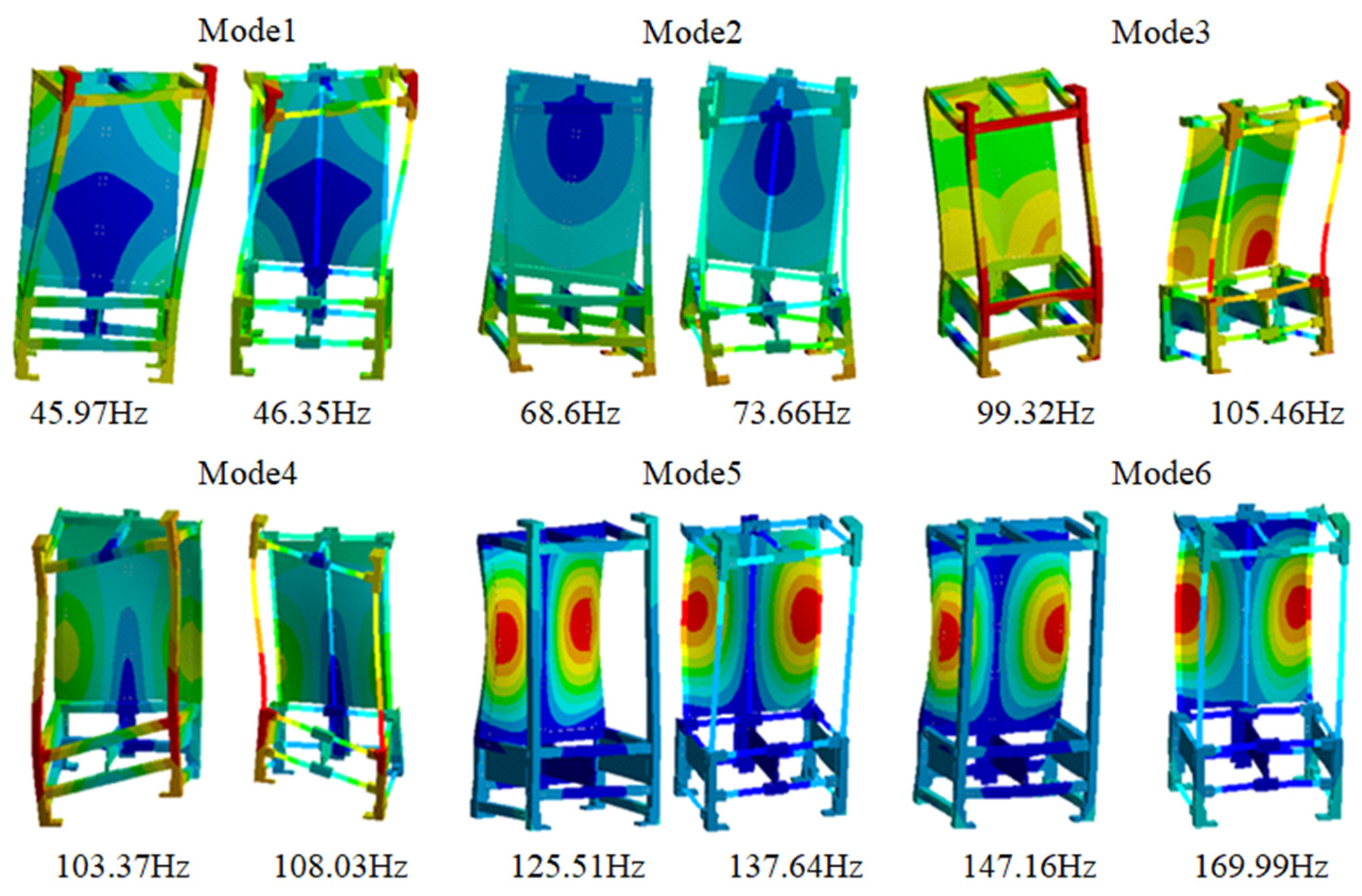
2.3. Calculated Modal Results

The free modal analysis was carried out on the experiment rack simulator. Ignoring the first six rigid body modes, the first six ones calculated the modal frequencies, and the mode shapes of the experiment rack simulator were obtained, as depicted in Figure 3. It can be observed that the first six mode shapes of the experiment rack simulator solid FE model are consistent with those of the mixed FE model, but the natural frequencies of the experiment rack simulator mixed FE model are higher than those of the solid FE model, and the higher the order is, the greater the frequency difference is.

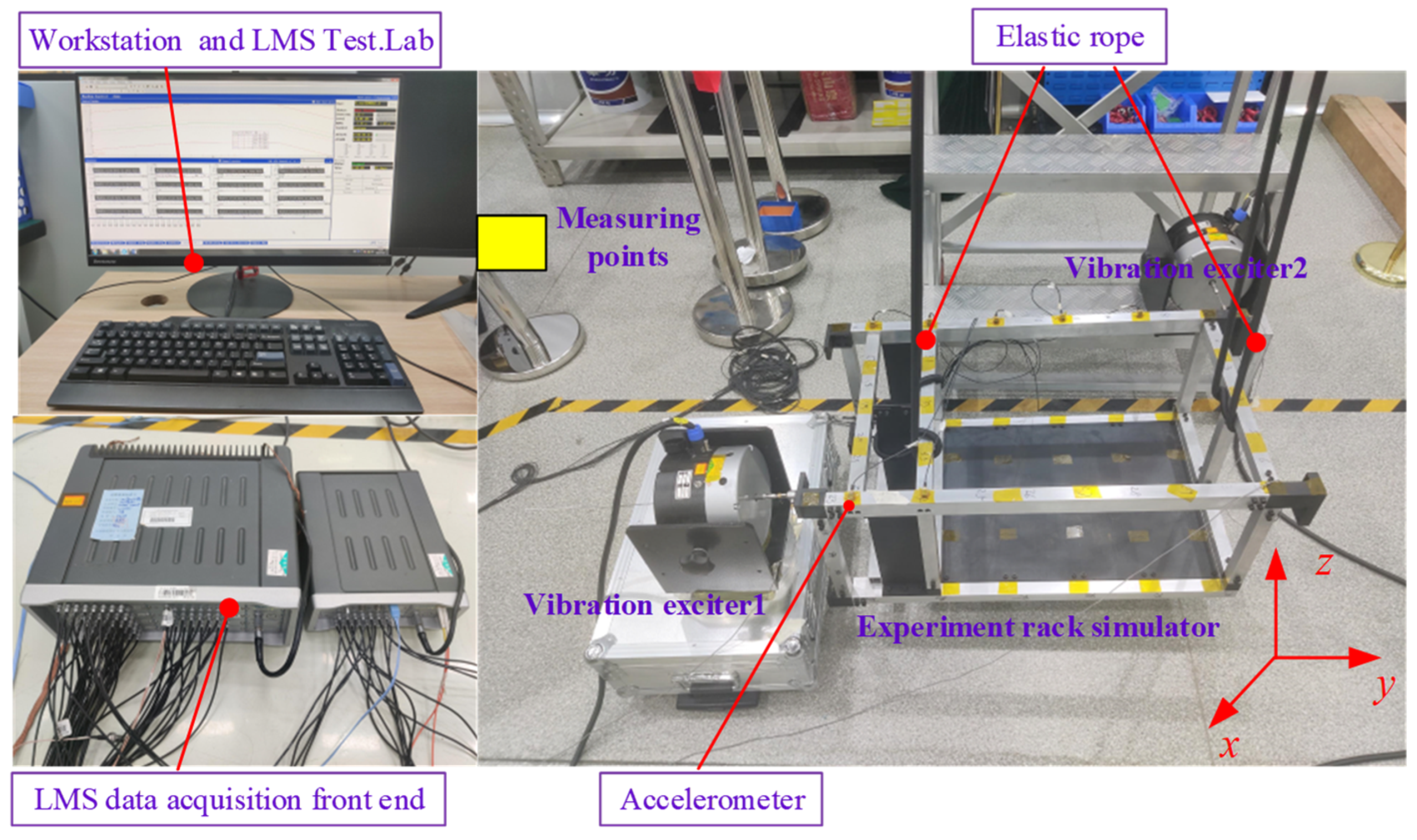
2.4. Measured Modal Results

A test system for the free modal analysis of the experiment rack simulator was built, as shown in Figure 4, including a mobile workstation, an LMS data acquisition front-end controller, a vibration exciter, triaxial accelerometers, and an elastic rope. The free boundary condition of the experiment rack simulator was simulated by means of elastic rope hoisting. Two vibration exciters were placed horizontally to excite the X-direction and Y-direction vibrations of the experiment rack simulator. The acceleration sensors were pasted onto the measuring points of the experiment rack simulator using glue (the yellow tapes are shown in Figure 4). Considering that the experiment rack simulator mainly consists of beam and plate structures, it was good enough to arrange a certain number of sensors evenly on each beam and plate to obtain the required mode shapes. The vibration environment of the experiment rack was mainly sinusoidal excitation at 4–200 Hz, and only the first six mode shapes were analyzed. The measured first six mode shapes and frequencies of the experiment rack simulator are shown in Figure 5.

2.5. Correlation Analysis
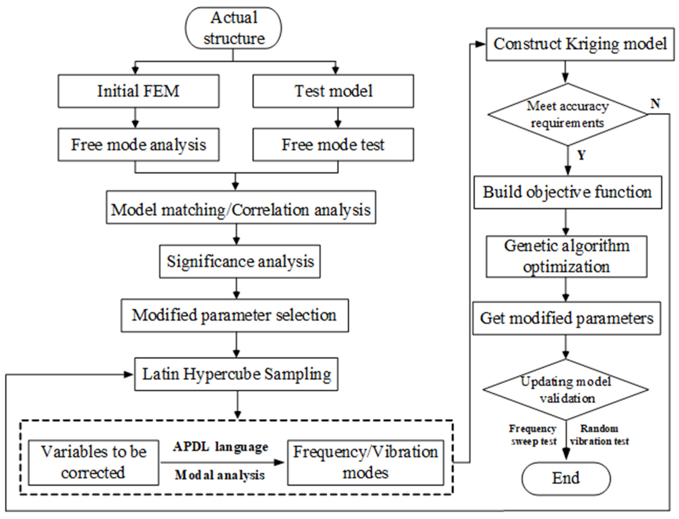
A frequency correlation analysis of the corresponding order was carried out on the experimental and calculated results. The frequency correlation represents the relative deviation between the test modal frequency (ωEMA) and the calculated frequency (ωFEA), and it is expressed as follows:
ε % = ( ω E M A ω F E A ) ω E M A
The ideal value of ε is zero. The greater the difference is between ε and 0, the worse the correlation is between the test modal frequency and calculated frequency. The first six order frequency correlation results of the experiment rack simulator were calculated, and they are listed in Table 2. It can be seen that the maximum error of the first six order natural frequency between the test frequencies and calculated frequencies of the finite solid FE model is 12.50%, and that between the test frequencies and calculated frequencies of the mixed FE model is 14.47%. In engineering, the established FE model can be considered to be accurate when the frequency error is within 5% [23]. Therefore, it is necessary to update the FE model of the experiment rack simulator.

3. RSM and FEMU

3.1. Fundamental of RSM

Currently, the commonly used response surface models include the quadratic polynomial, BP neural network, Gaussian radial basis function, Kriging model, and support vector machine. Based on polynomial interpolation, the Kriging model gives the maximum value of the unknown point through the variance change in the sample points, with high fitting accuracy [24]. The Kriging model assumes that the objective function and the design variables satisfy the following relationship.
Y = P T ( X ) β + S ( X )
where P(X) is the polynomial base function, β is the corresponding undetermined coefficient, S(X) is the fitting deviation function with a mean of 0 and a variance of σ2, and its covariance can be expressed as follows.
cov ( S ( u ) , S ( v ) ) = σ 2 R ( u , v )
where R(u, v) is the correlation function, but when the Gaussian correlation function is used, it can be expressed as follows.
R ( u , v ) = i = 1 n exp ( λ i d i 2 )
where λi represents the attenuation of the correlation between the sampling points with the increase in the distance di between the two points. The estimated values of the undetermined coefficient β and variance σ2 can be obtained from the sample point matrix X(Pj(xi)), the response value array Y(yi(X)), and the correlation matrix R(R(xi, xj)).
β ^ = ( X T R 1 X ) 1 X T R 1 Y
σ 2 = 1 N ( Y X β ^ ) T R 1 ( Y X ^ )
Using the maximum likelihood estimation method, the likelihood function takes the maximum value, and the corresponding λi is obtained.
L ( λ i ) = { N ln σ 2 + ln [ det ( R ) ] }
For an unknown point xi, an estimate of y(xi) can be given as follows.
y ( x i ) = P T ( x i ) β ^ + r T ( x i ) R 1 ( Y X β ^ )
where r(xi) represents its correlation array with sample points.
The key steps in the response surface analysis are data sampling and data fitting. The Latin sampling method ensures the orthogonality and uniformity of the sampling points. Combining the established RSM with GA, the correction of the FE model can be completed. The FEMU procedure is shown in Figure 6.

3.2. Significance Analysis

In the parameter modification method, appropriate modification parameters need to be selected, and a significance analysis can guide the selection of the correction parameters by eliminating the parameters that are insensitive to the response and retaining the highly significant parameters, which can greatly reduce the dimension of the response surface model and save on the computational costs [25]. To facilitate the finite element calculation, the complex contact between the connector and the aluminum profile is simplified into non-separated contact, which is the main reason for the difference between the simulation and the experiment. Therefore, a partition correction of the experiment rack simulator is performed, and the experiment rack simulator is divided into three modified areas based on the framed structure characteristics, where modified area 3 is the beam connection area, modified area 1 is the beam non-connection area, and modified area 2 is the non-beam structure area, as shown in Figure 7. The elastic modulus and density of the materials in the three regions are initially selected as the design parameters that needed to be corrected.
The orthogonal experimental design method is adopted, and there are three levels, 80%, 100%, and 120%, of the initial value of each modification parameter. The specific values of the modification parameters on each level are shown in Table 3. For the convenience of expressing the parameters that needed to be corrected, it is expressed as xi (i = 1,2, …, 5). According to the parameters and the number of levels, the orthogonal design test is carried out using the first five columns of the L18(37) orthogonal table, and the parameters that needed to be corrected are selected according to the orthogonal table. The material of the experiment rack simulator is parameterized by APDL language, and the first six natural frequencies of 18 tests are obtained. The six order frequencies are the corresponding natural frequencies after modal matching: the first, second, fourth, fifth, seventh, and ninth order frequencies of the finite element analysis. The orthogonal table and simulation results are shown in Table 4 and Table 5.
According to the calculated frequencies in Table 5, the range analysis and variance analysis of five parameters were performed, and the significance analysis results are shown in Table 6, where 1 indicates that the parameter has a significant effect on the modal frequency of corresponding order, and 0 indicates that the parameter has no significant effect on the modal frequency of the corresponding order. Therefore, it can be concluded that factors X1, X3, and X5 have highly significant effects, while X2 and X4 have non-significant effects. Therefore, the elastic modulus of the non-connected beams, connected beams, non-beam structures, and the density of the non-beam structures were selected as the parameters that needed to be corrected.

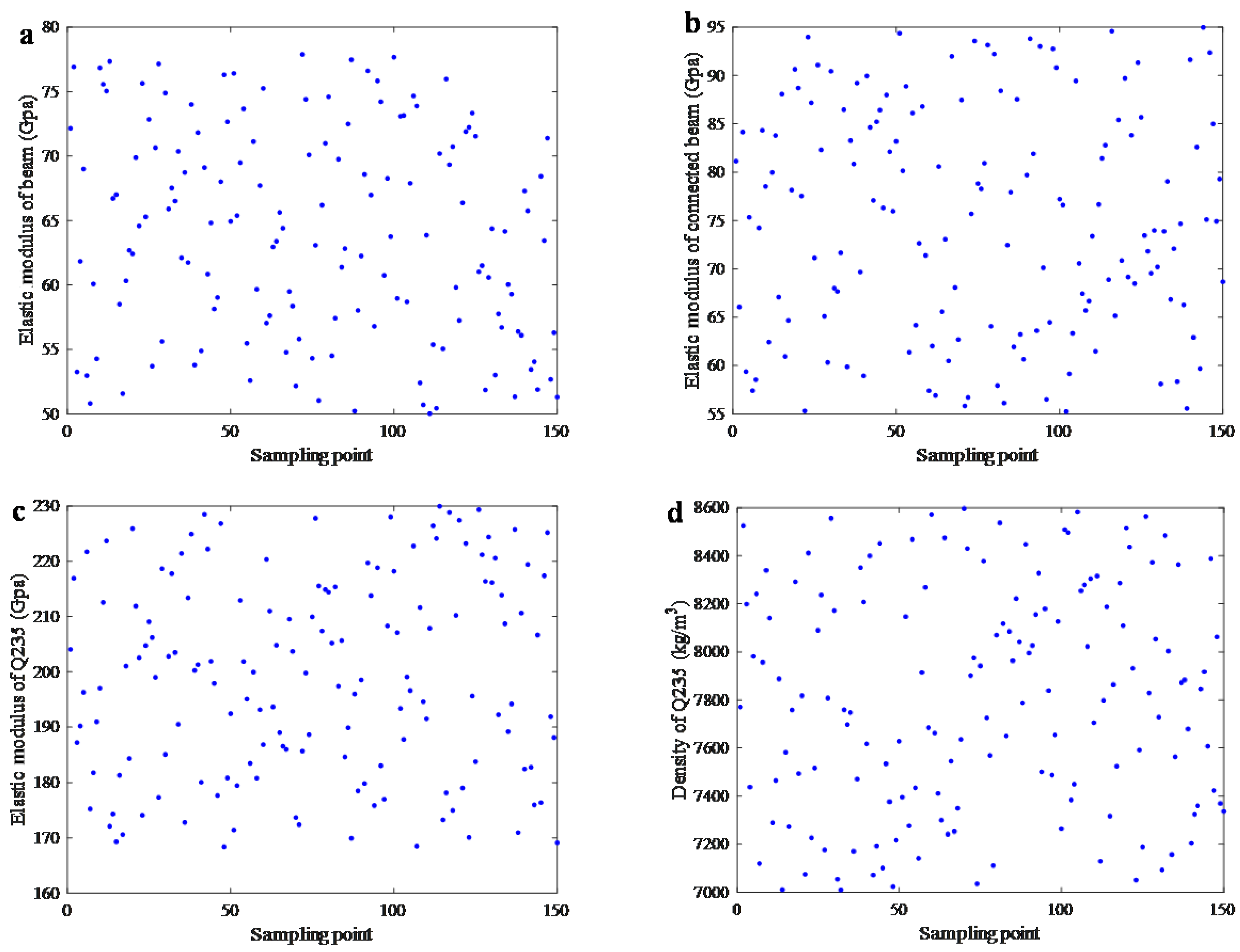
3.3. Establishment of RSM
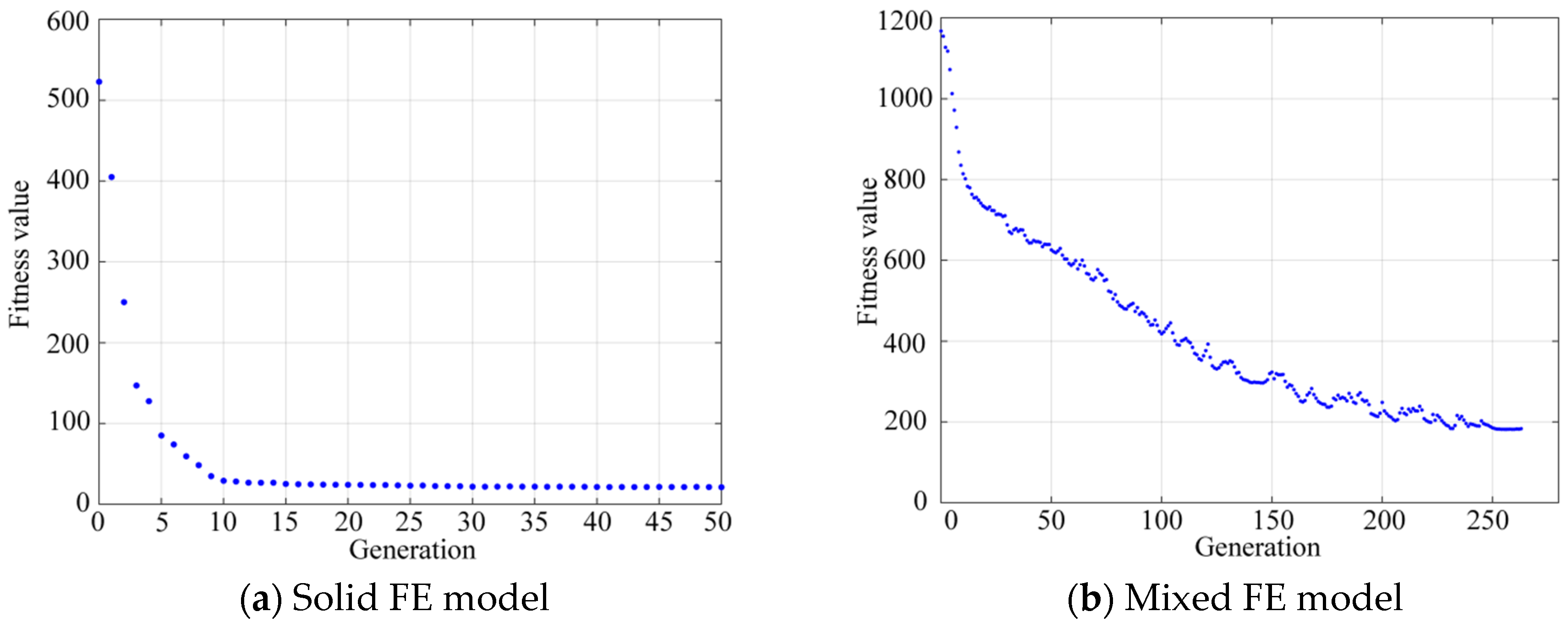
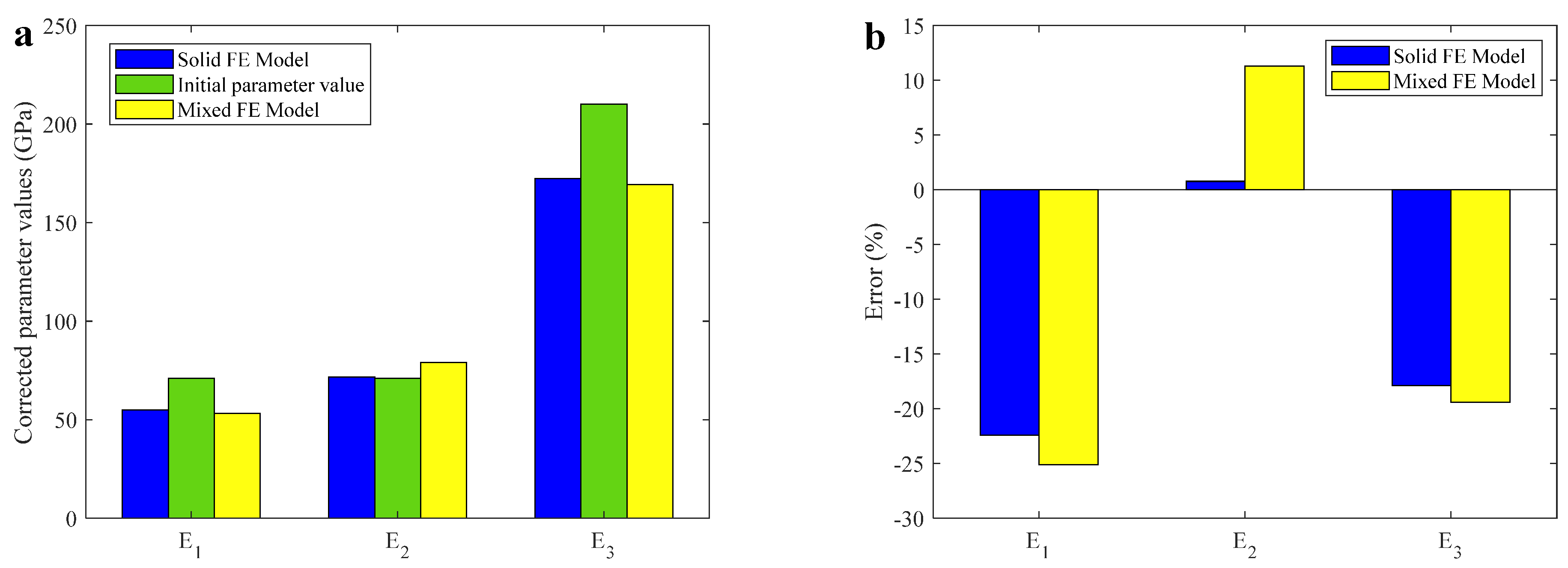
According to the significance analysis results, the elastic modulus of the non-connected beams, connected beams, non-beam structures, and the density of non-beam structures were selected as the parameters that needed to be corrected. According to the actual elastic modulus and density values of 6063 and Q235, respectively, it was determined that the elastic modulus of the non-connected beams ranges from 50 GPa to 78 GPa, the elastic modulus of the non-beam structure ranges from 168 GPa to 230 GPa, the elastic modulus range of connected beams is from 55 GPa to 95 GPa, and the non-beam structure density ranges from 7000 kg/m3 to 8600 kg/m3. Within the above range, 150 sampling points were sampled via the Latin hypercube method, as shown in Figure 8.
The 150 sets of material parameters obtained by the Latin hypercube method were imported into ANSYS, and the first six orders of natural frequency corresponding to different material parameters of the solid FE model and the mixed FE model were calculated, respectively, as shown in Table A1(a,b).
The material parameters obtained by the Latin hypercube method and the corresponding six orders of natural frequencies were imported into the MATLAB software, and the RSM between the objective functions and design variables was constructed according to the Gaussian correlation function and the Kriging model. To verify the established RSM’s accuracy, the design variables within the same range of the values were sampled via the Latin hypercube method, again, to obtain three verification groups, and the objective function values obtained via FEM and RSM are listed in Table A2(a,b). It can be seen that relative errors of the objective function values between the RSM and two FE models are both within 0.5%, and the established RSM can be considered to have sufficient accuracy.

3.4. FEMU

Taking the square sum of the relative error of the first six order frequencies obtained by the constructed Kriging surrogate model and those obtained by the experiment as the objective function, GA was used to optimize the solution. The objective function is given below.
Min f i t ( x ) = Min i = 1 n ( E R ( f k r i g i , f r i ) + ( 1 M A C ( ϕ k r i g i ϕ r i ) )
where x is the parameter that had to be corrected; n is the modal order; fkrigi and φkrigi are the natural frequency and mode shape of the i-th order calculated by the Kriging model, respectively; fri and φri are the natural frequency and mode shape of the i-th order obtained in the experiment.
In engineering tests, if the modal shape is used as the correction target, a narrowing modal shape error may cause the correction result to be inconsistent with the real structure, increase the number of calculations in the optimization solution, and reduce the solution’s efficiency, and hence, in the process of model correction of the actual structure, only the modal frequency was used as a correction objective function, and the mode shape was used as the evaluation index [26]. The objective function of modal frequency is constructed below.
Min f i t ( x ) = Min i = 1 n ( E R ( f k r i g i , f r i ) = Min i = 1 n | f k r i g i f r i f r i | 2
In the optimization process, the setting variable ranges were 50–78 GPa, 55–95 GPa, 168–230 GPa, and 7000 kg/m3–8600 kg/m3. The optimal solution was obtained via GA, the initial population was set to 100, the crossover operator was set to 08, the mutation operator was set to 0.005, and the maximum number of iterations was set to 300. Figure 9 shows the change curve of the objective function values with the iterative optimization. It can be seen from Figure 9a that for the solid FE model, when the 10th iteration was performed, the fitness value converged, and the corresponding elastic modulus of the non-connected beams is 55.04 GPa, the elastic modulus of the connected beams is 71.55 GPa, the elastic modulus of the non-beam structures is 172.40 GPa, and the density of the non-beam structures is 7822 kg/m3; the objective function value is the smallest one. It can be seen from Figure 9b that for the mixed FE model, when the 251st iteration was performed, the fitness value converged, and the corresponding elastic modulus of the non-connected beams is 53.18 GPa, the elastic modulus of the connected beams is 79.04 GPa, the elastic modulus of the non-beam structures is 169.27 GPa, and density of the non-beam structures is 8140 kg/m3; the objective function value is the smallest one.
The corrected parameter values before and after the optimization are shown in Figure 10. It can be observed that after the FEMU of the solid FE model and mixed FE model of the experiment rack simulator, the modification parameters E1 and E3 were significantly reduced, and the modification parameter E2 was slightly increased. This is because the rigidity of the Aluminum profile part fixed on the connection block by bolts is greater than that of the Aluminum profile part without bolts between the layers, which is consistent with the actual situation.
The optimized material parameters were recalculated, and the calculated first six order frequencies are shown in Figure 11. It can be seen that the first six order frequency errors of each order are within 5%, indicating that the FEMU model of the experiment rack simulator is in good agreement with the experimental model.

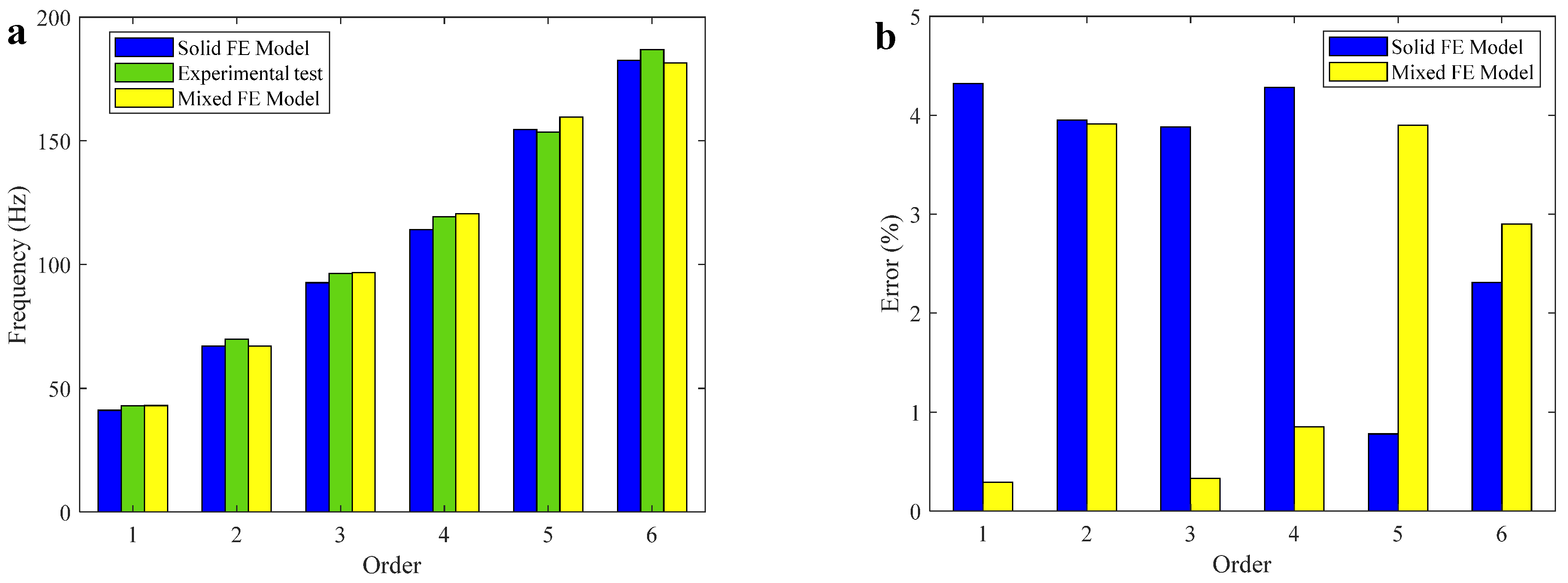
4. Experimental Validation for FEMU

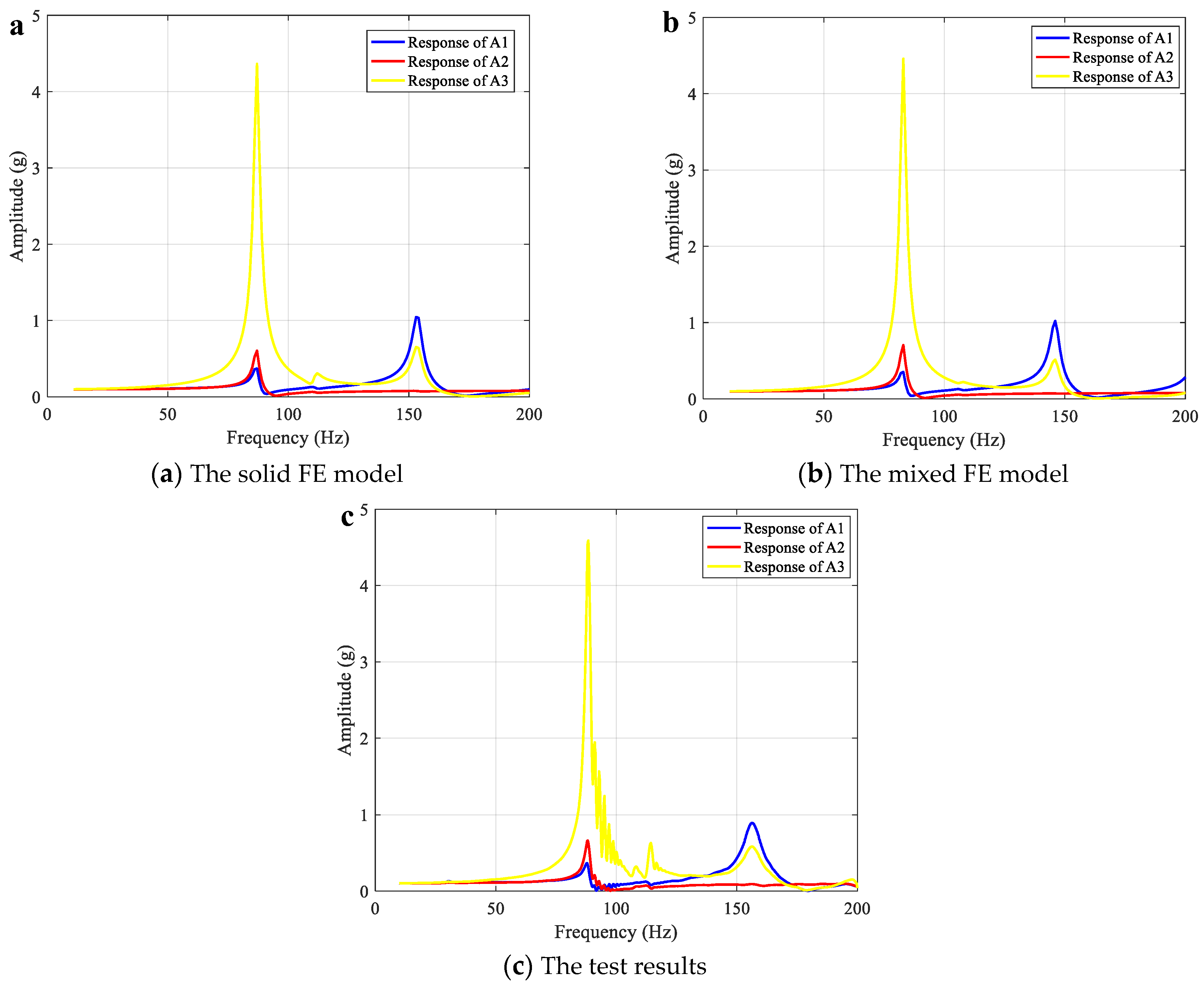
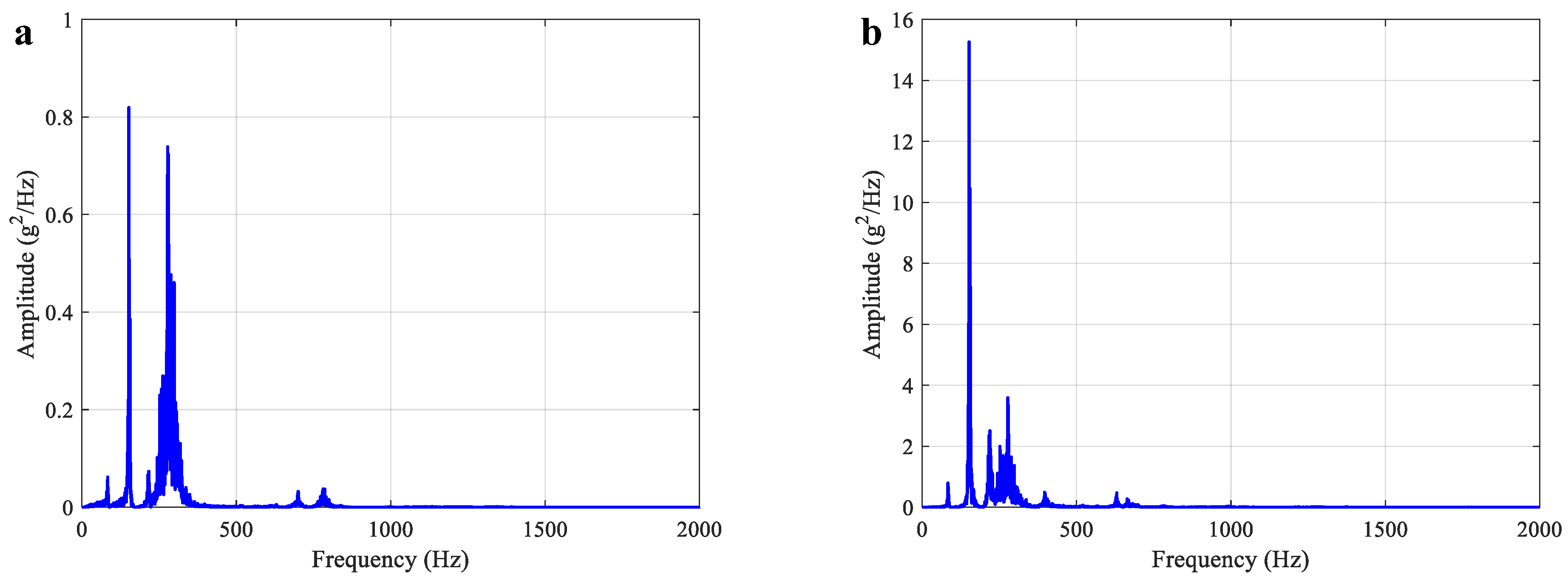
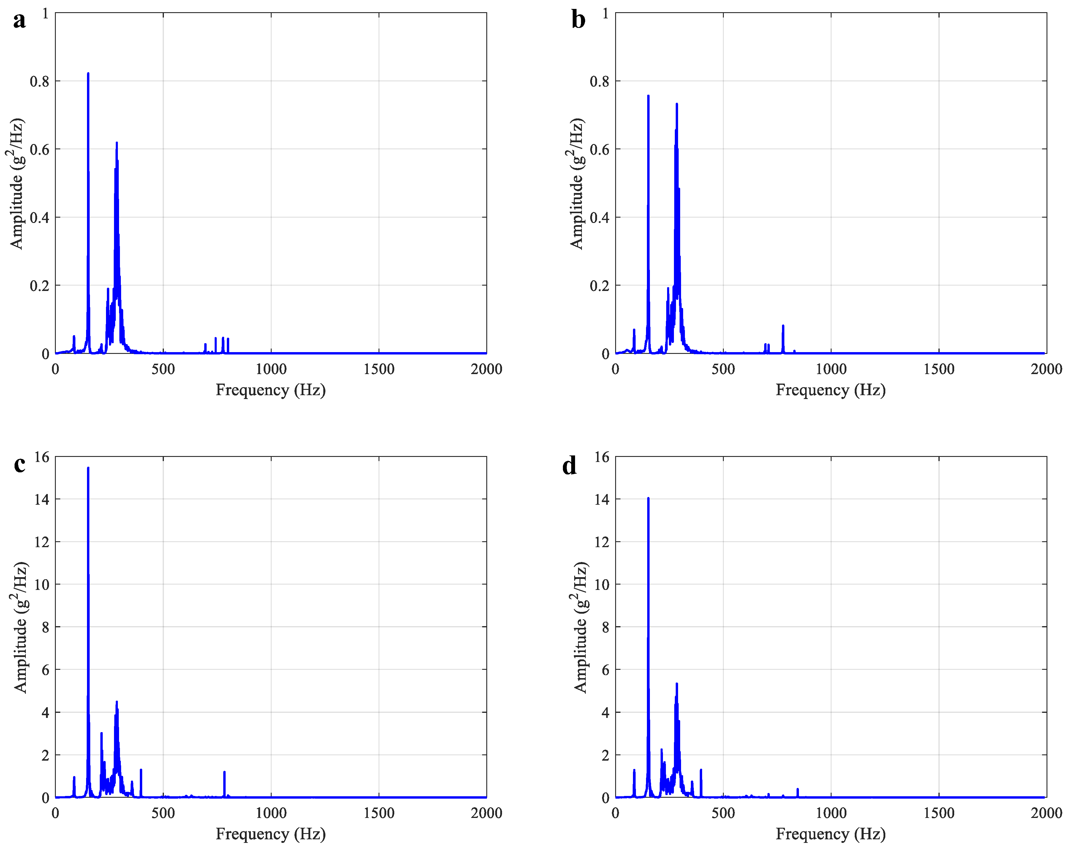
4.1. Sweep Frequency Test

The accuracy of the two updated FE models was first verified by the sweep frequency test. The experiment rack simulator was excited along the X direction, the excitation amplitude was 0.1 g, and the sine sweep frequency range was 4–200 Hz. The vibration response of three measuring points, A1, A2, and A3, were arranged. The test system and measuring points’ layout are shown in Figure 12. The simulation results of two FE models and experimental results under the sweep frequency condition are shown in Figure 13 and Table 7. It can be observed that the test and calculated vibration responses are in good agreement. The error of the first order resonance frequency value is within 5%, and the response error corresponding to the first order resonance frequency is within 5%. Therefore, the FEMU models can be used to predict the vibration response of actual structures.

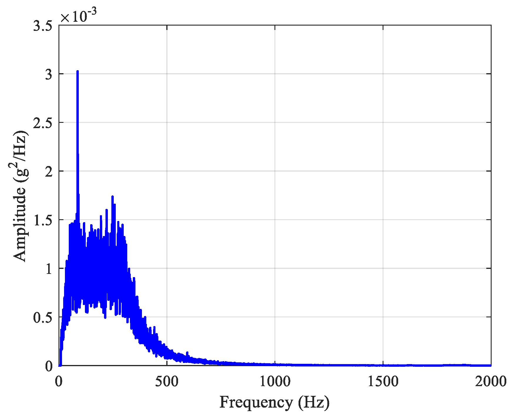
4.2. Random Vibration Test

The accuracy of the two updated FE models was further verified by a random vibration test. The specific settings were as follows: the random vibration range was 10–2000 Hz, the excitation direction was the X direction, and the vibration response of two measuring points, A1 and A4, were arranged. The input acceleration power spectral density (PSD) is shown in Figure 14. The simulation results of the two FE models and experimental results under random excitation are shown in Figure 15 and Figure 16 and Table 8. It can be observed that the test and calculated random vibration responses of point A1 and point A4 are in good agreement, and the root mean square (RMS) error of the vibration response is within 7%. Therefore, the FEMU models can also be used to predict the random vibration response of the actual structures. Both the random vibration and sweep frequency test results verify the accuracy of the proposed updated FE models.

5. Conclusions

In this paper, the solid FE model and the mixed FE model of the experiment rack simulator were established, and the FEMU of the experiment rack simulator was conducted by a combination of RSM and GA. The main conclusions are as follows:
(1) First, according to the structural form and connection characteristics of the experiment rack, the solid FE model and the mixed FE model of the experiment rack simulator were established. The number of elements and nodes in the solid FE model was 2.3 times higher than that of the mixed FE model. The maximum frequency error of the mixed FE model was smaller than that of the solid FE model, which indicates that the mixed FE model is more accurate and efficient.
(2) Then, partition modification was adopted to determine the main modification areas, and the experiment rack simulator was divided into three modification areas. A further significance analysis of the modification parameters of three modification areas was performed, and four sensitive design variables were selected. The Latin hypercube sampling method was utilized to sample the design variables points and the Kriging response surface model between the parameters that needed to be corrected, and the modal parameters of the experiment rack simulator were established and optimized by GA, thereby improving the calculation efficiency and accuracy of FEMU models.
(3) Finally, frequency sweep and random vibration tests were carried out on an experimental rack simulator. The results show that the vibration response error of the experiment rack simulator under sweep frequency excitation was within 5%, and the RMS errors of vibration response of the experiment rack simulator under random excitation were within 7%. The proposed FEMU method of experimental rack simulator is precise and efficient, and it can thus help us to predict the vibration behavior of a real structure.

Author Contributions

Conceptualization, methodology: Q.H.; software, validation, formal analysis, investigation, writing—original draft preparation: Q.Z.; project administration, supervision: J.L.; formal analysis, investigation: C.Y. All authors have read and agreed to the published version of the manuscript.

Funding

This research was funded by the National Natural Science Foundation of China, grant number 12072069.

Institutional Review Board Statement

Not applicable.

Informed Consent Statement

Not applicable.

Data Availability Statement

Not applicable.

Acknowledgments

The authors would like to acknowledge Zhaodong Fang and Fukun Li for their assistance with the experiments.

Conflicts of Interest

The authors declare no conflict of interest.

Nomenclature

ωFEAThe calculated frequency via FEM.
ωEMAThe test modal frequency.
fkrigiThe natural frequency of the i-th order calculated by the Kriging model.
φkrigiThe mode shape of the i-th order calculated by the Kriging model.
friThe natural frequency of the i-th order obtained by the experiment.
φriThe mode shape of the i-th order obtained by the experiment.
P(X)The polynomial base function.
βThe corresponding undetermined coefficient.
S(X)The fitting deviation function with a mean of 0 and a variance of σ2.
R(u, v)The correlation function.

Appendix A

Table A1. (a). Design variable sampling points of solid FE model and corresponding first six natural frequencies. (b). Design variable sampling points of mixed model and corresponding first six natural frequencies.
(a)
ParameterX1X2……X149X150
E1 (GPa)72.1576.95……56.2951.30
E2 (GPa)81.1466.05……79.2968.65
E3 (GPa)204.05216.93……188.10169.11
D1 (kg/m3)7769.588525.61……7369.897336.70
f1 (Hz)49.6147.44……46.9344.69
f2 (Hz)75.4672.20……72.0368.63
f3 (Hz)110.98106.22……105.0499.90
f4 (Hz)139.85135.20……133.18126.68
f5 (Hz)183.30174.78……174.63165.80
f6 (Hz)204.86196.96……200.84190.96
(b)
ParameterX1X2……X149X150
E1 (GPa)72.1576.92……56.3051.30
E2 (GPa)81.1566.06……79.2968.65
E3 (GPa)204.05216.94……188.10169.12
D1 (kg/m3)7769.588525.61……7369.897336.70
f1 (Hz)45.4842.51……42.3540.75
f2 (Hz)70.4667.07……67.3964.55
f3 (Hz)102.2896.35……96.3492.54
f4 (Hz)123.10118.67……120.20114.28
f5 (Hz)169.50160.61……161.02154.21
f6 (Hz)192.58190.04……192.95183.45
Table A2. (a). Relative errors of objective function values between RSM and solid FE model. (b). Relative errors of objective function values between RSM and mixed model.
(a)
X1X2X3
E1 (GPa)77.4555.1762.84
E2 (GPa)72.7190.7756.63
E3 (GPa)177.75193.31218.67
D1 (kg/m3)8271.907009.007859.90
FEMRSMErrorFEMRSMErrorFEMRSMError
f1 (X)48.0047.800.4248.3948.210.3845.6545.680.06
f2 (X)72.4872.190.3974.4674.180.3870.0970.130.06
f3 (X)107.21106.780.41108.33107.950.36102.06102.130.06
f4 (X)133.28132.730.41137.56137.020.39132.36132.410.03
f5 (X)175.23174.520.41180.92180.190.40169.26169.370.06
f6 (X)189.44188.490.50209.93208.880.50198.57198.810.12
(b)
X1X2X3
E1 (GPa)77.4555.1762.84
E2 (GPa)72.7190.7756.63
E3 (GPa)177.75193.31218.67
D1 (kg/m3)8271.907009.007859.90
FEMRSMErrorFEMRSMErrorFEMRSMError
f1 (X)42.1342.210.1847.8147.770.0941.4141.460.12
f2 (X)65.6265.770.2473.9473.880.0865.8165.870.09
f3 (X)94.6494.850.23107.47107.380.0994.2294.310.10
f4 (X)115.09115.400.27128.89128.790.08116.98117.090.10
f5 (X)157.37157.740.23177.86177.710.09157.17157.340.11
f6 (X)182.14182.680.30200.79200.650.07187.94188.050.06

References

  1. Pelfrey, J.; Jordan, L. An EXPRESS Rack overview and support for microgravity research on the International Space Station (ISS). In Proceedings of the 46th AIAA Aerospace Sciences Meeting and Exhibit, Reno, Nevada, 7–10 January 2008; p. 819. [Google Scholar]
  2. Grodsinsky, C.M.; Whorton, M.S. Survey of active vibration isolation systems for microgravity applications. J. Spacecr. Rockets 2000, 37, 586–596. [Google Scholar] [CrossRef] [Green Version]
  3. Ping, W. China Manned Space Programme: Its Achievements and Future Developments; China Manned Space Agency: Beijing, China, 2016. [Google Scholar]
  4. Liu, W.; Zhang, B.; Shen, C. Stability analysis for spatial autoparametric resonances of framed structures. Int. J. Struct. Stab. Dyn. 2022, 22, 2250065. [Google Scholar] [CrossRef]
  5. Song, Y.; Hartwigsen, C.J.; McFarland, D.M. Simulation of dynamics of beam structures with bolted joints using adjusted Iwan beam elements. J. Sound. Vib. 2004, 273, 249–276. [Google Scholar] [CrossRef]
  6. Hartwigsen, C.J.; Song, Y.; McFarland, D.M. Experimental study of non-linear effects in a typical shear lap joint configuration. J. Sound. Vib. 2004, 277, 327–351. [Google Scholar] [CrossRef]
  7. Genbei, Z.; Chaoping, Z.; Xiaowei, W. Finite element model updating of a framed structure with bolted joints. Eng. Mech. 2014, 31, 26–33. [Google Scholar]
  8. Chang, H.; Ma, R. Simulation of ducts and passages with negative-area spatial truss element in 3d creep analysis of reinforced concrete and prestressed concrete bridge. KSCE J. Civ. Eng. 2021, 25, 2053–2064. [Google Scholar] [CrossRef]
  9. Sliseris, J.; Gaile, L.; Pakrastins, L. Extended multiscale FEM for design of beams and frames with complex topology. Appl. Math. Model. 2019, 69, 77–92. [Google Scholar] [CrossRef]
  10. Yuan, Q. Alternating direction method for structure-persevering finite element model updating problem. Appl. Math. Comput. 2013, 223, 461–471. [Google Scholar] [CrossRef]
  11. Friswell, M.I.; Inman, D.J.; Pilkey, D.F. Direct updating of damping and stiffness matrices. AIAA J. 1998, 36, 491–494. [Google Scholar] [CrossRef] [Green Version]
  12. Fox, R.L.; Kapoor, M.P. Rates of change of eigenvalues and eigenvectors. AIAA J. 2012, 6, 2426–2429. [Google Scholar] [CrossRef]
  13. Friswell, M.I.; Mottershead, J.E.; Ahmadian, H. Finite element model updating using experimental test data: Parametrization and regularization. Philos. Trans. R. Soc. Lond. Ser. A-Math. Phys. Eng. Sci. 2001, 359, 169–186. [Google Scholar] [CrossRef]
  14. Liu, Y.; Duan, Z.D. Fuzzy finite element model updating of bridges by considering the uncertainty of the measured modal parameters. Sci. China Technol. Sci. 2012, 55, 3109–3117. [Google Scholar] [CrossRef]
  15. Hızal, Ç.; Turan, G. A two-stage Bayesian algorithm for finite element model updating by using ambient response data from multiple measurement setups. J. Sound Vib. 2020, 469, 115139. [Google Scholar] [CrossRef]
  16. Hadjian-Shahri, A.H.; Ghorbani-Tanha, A.K. Damage detection via closed-form sensitivity matrix of modal kinetic energy change ratio. J Sound Vib. 2017, 401, 268–281. [Google Scholar] [CrossRef]
  17. Mottershead, J.E.; Link, M.; Friswell, M.I. The sensitivity method in finite element model updating: A tutorial. Mech. Syst. Signal Process. 2011, 25, 2275–2296. [Google Scholar] [CrossRef]
  18. Cao, Z.; Fei, Q.; Jiang, D. A sensitivity-based nonlinear finite element model updating method for nonlinear engineering structures. Appl. Math. Model. 2021, 100, 632–655. [Google Scholar] [CrossRef]
  19. Izham, M.H.N.; Abdullah, N.A.Z.; Zahari, S.N. Structural dynamic investigation of frame structure with bolted joints. MATEC Web of Conferences. EDP Sci. 2017, 90, 01043. [Google Scholar]
  20. Umar, S.; Bakhary, N.; Abidin, A.R.Z. Response surface methodology for damage detection using frequency and mode shape. Measurement 2018, 115, 258–268. [Google Scholar] [CrossRef]
  21. Niu, J.; Zong, Z.H.; Chu, F.P. Damage identification method of girder bridges based on finite element model updating and modal strain energy. Sci. China Technol. Sci. 2015, 58, 701–711. [Google Scholar] [CrossRef]
  22. Zhang, K. Study on Multi-Scale Modeling Method Based on Multi-Point Constrained Equation; Chongqing University: Chongqing, China, 2019. [Google Scholar]
  23. Lin, L.; Ding, Z.; Zeng, J. Research on the transmission loss of the floor aluminum profile for the high-speed train based on FE-SEA hybrid method. J. Vibroeng. 2016, 18, 1968–1981. [Google Scholar] [CrossRef] [Green Version]
  24. Kleijnen, J.P. Kriging metamodeling in simulation: A review. Eur. J. Oper. Res. 2009, 192, 707–716. [Google Scholar] [CrossRef] [Green Version]
  25. Wu, H.R.; Zheng, H.L.; Wang, W.K. A method for tracing key geometric errors of vertical machining center based on global sensitivity analysis. Int. J. Adv. Manuf. Technol. 2020, 106, 3943–3956. [Google Scholar] [CrossRef]
  26. Gres, S.; Dhler, M.; Mevel, L. Uncertainty quantification of the modal assurance criterion in operational modal analysis. Mech. Syst. Sig. Process. 2021, 152, 107457. [Google Scholar] [CrossRef]
Figure 1. Composition of the experiment rack simulator.
Aerospace 10 00079 g001
Figure 2. Two FE models of the experiment rack simulator. (a) Solid FE model. (b) Mixed FE model.
Aerospace 10 00079 g002
Figure 3. Calculated modal shapes of the experiment rack simulator.
Aerospace 10 00079 g003
Figure 4. Free modal test site of experiment rack simulator.
Aerospace 10 00079 g004
Figure 5. Free modal test results of the experiment rack simulator.
Aerospace 10 00079 g005
Figure 6. Flow chart of FEMU.
Aerospace 10 00079 g006
Figure 7. Modified area division and modified parameters of experiment rack simulator.
Aerospace 10 00079 g007
Figure 8. Sample points of parameters that had to be corrected. (a) Elastic modulus of beam. (b) Elastic modulus of connected beam. (c) Elastic modulus of Q235. (d) Density of Q235.
Aerospace 10 00079 g008
Figure 9. The change curve of objective function value with the number of iterations.
Aerospace 10 00079 g009
Figure 10. Parameter changes before and after correction. (a) Parameter values before and after correction. (b) Parameter change rate before and after correction.
Aerospace 10 00079 g010
Figure 11. The frequency errors between updated model and experimental results. (a) The frequency of updated model and experimental results. (b) The frequency error of two updated models.
Aerospace 10 00079 g011
Figure 12. Test site of the experiment rack simulator. (a) Test rig. (b) Measured points’ layout.
Aerospace 10 00079 g012
Figure 13. Frequency sweep curves for two FE models of experiment rack simulator and measured results.
Aerospace 10 00079 g013
Figure 14. Random vibration load spectrum of experiment rack simulator.
Aerospace 10 00079 g014
Figure 15. Measured random vibration response of experiment rack simulator. (a) Point A1. (b) Point A4.
Aerospace 10 00079 g015
Figure 16. Calculated random vibration response of two FE models of experiment rack simulator. (a) Point A1 for solid FE model. (b) Point A1 for mixed FE model. (c) Point A4 for solid FE model. (d) Point A4 for mixed FE model.
Aerospace 10 00079 g016
Table 1. Specific settings of two FE models of the experimental rack simulator.
FE ModelComponentUnit TypeMaterialNumber of ElementsNumber of Nodes
Mixed
FE model
BackplaneShell181Q23527,59457,961
Drawer boardShell181Q235
BeamBeam1886063
BoltBeam188Structural steel
OthersSolid186Q235
Fine solid
FE model
BackplaneSolid186Q23565,883135,294
Drawer boardSolid186Q235
BeamSolid1866063
BoltSolid186Structural steel
OthersSolid186Q235
Table 2. Frequency correlation analysis results.
Modal OrderModal Frequency
Test (Hz)Fine Solid FEM (Hz)Error (%)Mixed FEM (Hz)Error (%)
142.9045.987.1646.358.03
269.8268.601.7573.665.50
396.4299.323.00105.038.92
4119.26125.515.24135.6413.73
5153.47172.7712.50175.6714.47
6186.89194.033.82200.177.10
Table 3. Values for each level of the parameters that needed to be corrected.
ParameterTypeLevel 1Level 2Level 3Expression
Elastic modulus (Pa)E15.68 × 10107.1 × 10108.52 × 1010X1
E21.68 × 10112.1 × 10112.52 × 1011X2
E35.68 × 10107.1 × 10108.52 × 1010X3
Density (kg/m3)D1221627703324X4
D2628078509420X5
Table 4. The 7-factor, 3-level orthogonal table.
Test NumberFactor
1234567
11111111
21222222
31333333
42112233
52223311
62331122
73121323
83232131
93313212
101133221
111211332
121322113
132123132
142231213
152312321
163132312
173213123
183321231
Data 1–3 in the table refer to the level number of parameters.
Table 5. The first six natural frequencies after finite element simulation matching.
Test NumberOrder
1st Order (Hz)2nd Order (Hz)3rd Order (Hz)4th Order (Hz)5th Order (Hz)6th Order (Hz)
148.5974.18108.44137.97178.98204.38
245.5670.19102.09131.06169.95199.07
343.1066.9296.89125.46162.36193.54
446.0069.55102.36129.38167.72185.40
544.1867.3398.70125.67163.20185.35
656.0585.94125.66161.56209.49243.31
746.8370.48105.21127.75169.34175.77
856.6485.42125.58159.93208.27232.17
948.6874.06107.86142.55179.60210.00
1044.9168.5799.34126.00166.29189.44
1141.7864.5394.50120.19154.92179.99
1250.4278.06112.23148.44189.49226.97
1350.7476.38111.55143.02185.28209.34
1450.4476.97113.62141.73186.71207.67
1544.1067.7999.01128.58163.52191.62
1647.2971.04105.80128.35171.34178.49
1752.1878.66114.58151.38190.83221.34
1852.3079.72117.56149.96193.32218.22
Table 6. Significance analysis of parameters that needed to be corrected.
Parameter1st Order2nd Order3rd Order4th Order5th Order6th Order
X1111111
X2000101
X3111011
X4000000
X5111111
Table 7. Simulation and experimental vibration response under sweep frequency.
Measuring PointsTestSolid FE ModelErrorMixed ModelError
Amplitude
(g)
Frequency (Hz)Amplitude
(g)
Frequency (Hz)Amplitude (%)Frequency (%)Amplitude
(g)
Frequency (Hz)Amplitude (%)Frequency
(%)
A10.3788.850.38873.602.080.36851.604.33
A20.6688.110.64874.201.260.70855.293.53
A34.5988.374.45873.001.554.56850.653.81
Table 8. Random vibration test and simulation results of the experimental rack.
Measuring PointMeasured RMS (g)RMS of Solid FE Model (g)Error (%)RMS of Mixed FE Model (g)Error (%)
A14.244.093.504.506.26
A412.6213.325.5613.033.23
Disclaimer/Publisher’s Note: The statements, opinions and data contained in all publications are solely those of the individual author(s) and contributor(s) and not of MDPI and/or the editor(s). MDPI and/or the editor(s) disclaim responsibility for any injury to people or property resulting from any ideas, methods, instructions or products referred to in the content.

