


Does the Spatial Pattern of Plants and Green Space Affect Air Pollutant Concentrations? Evidence from 37 Garden Cities in China
 ,
,
Abstract
:1. Introduction
2. Results
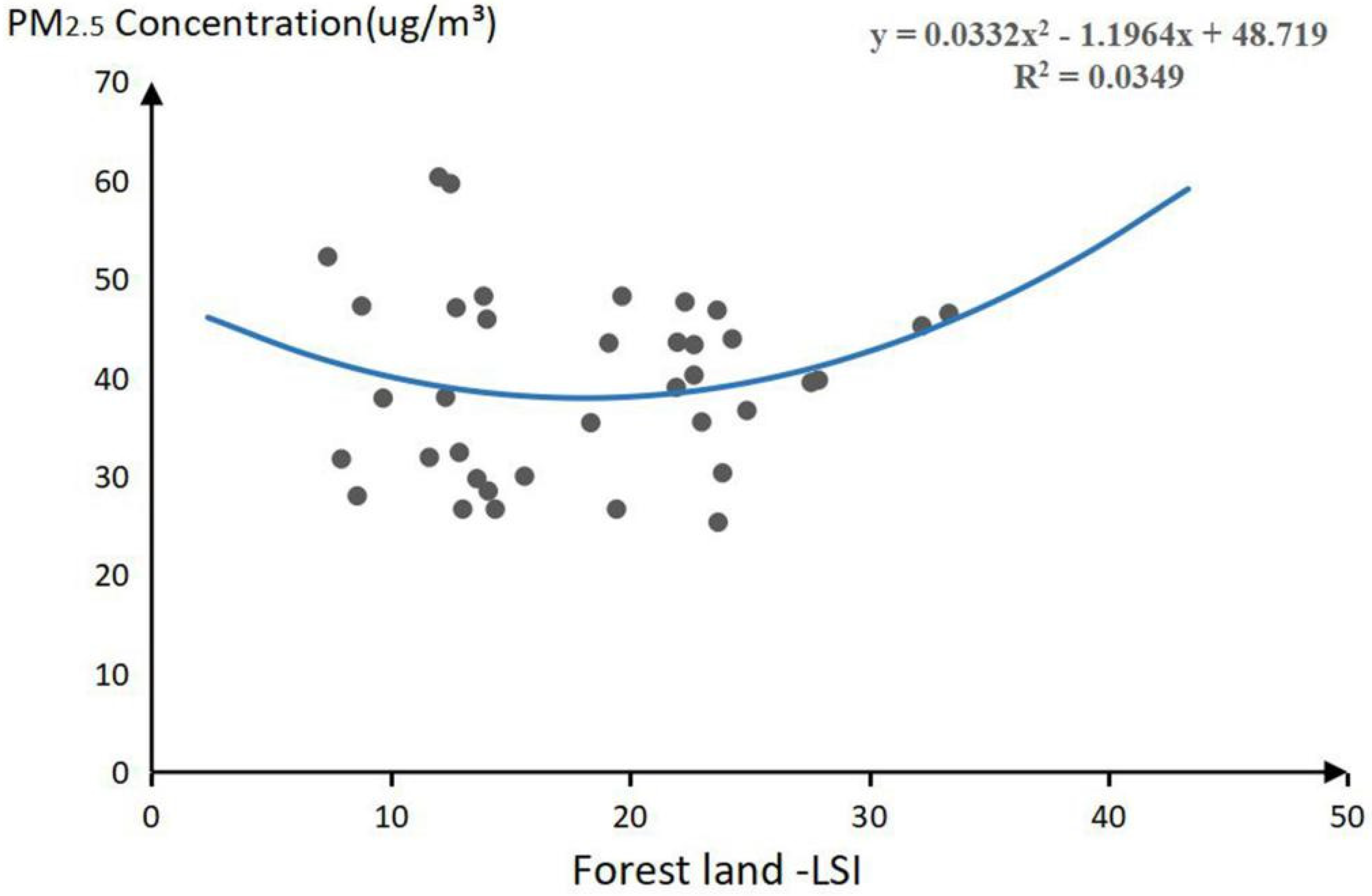
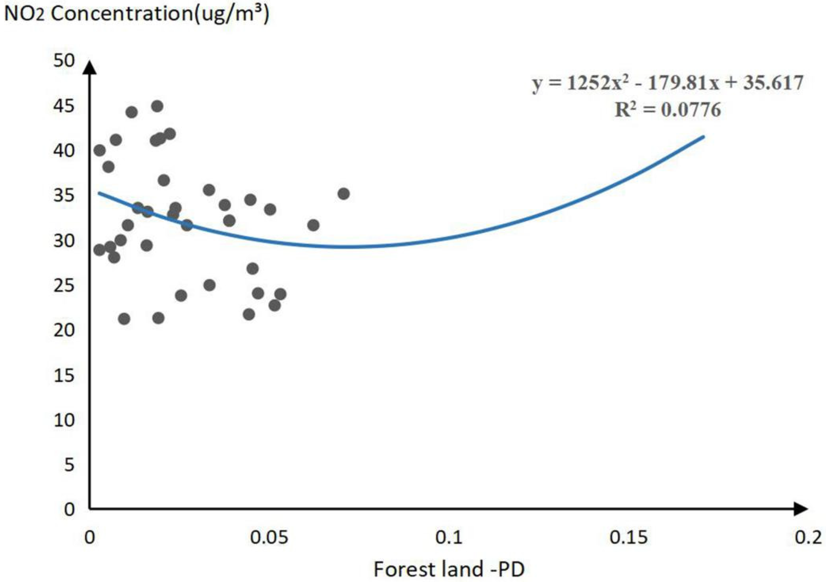
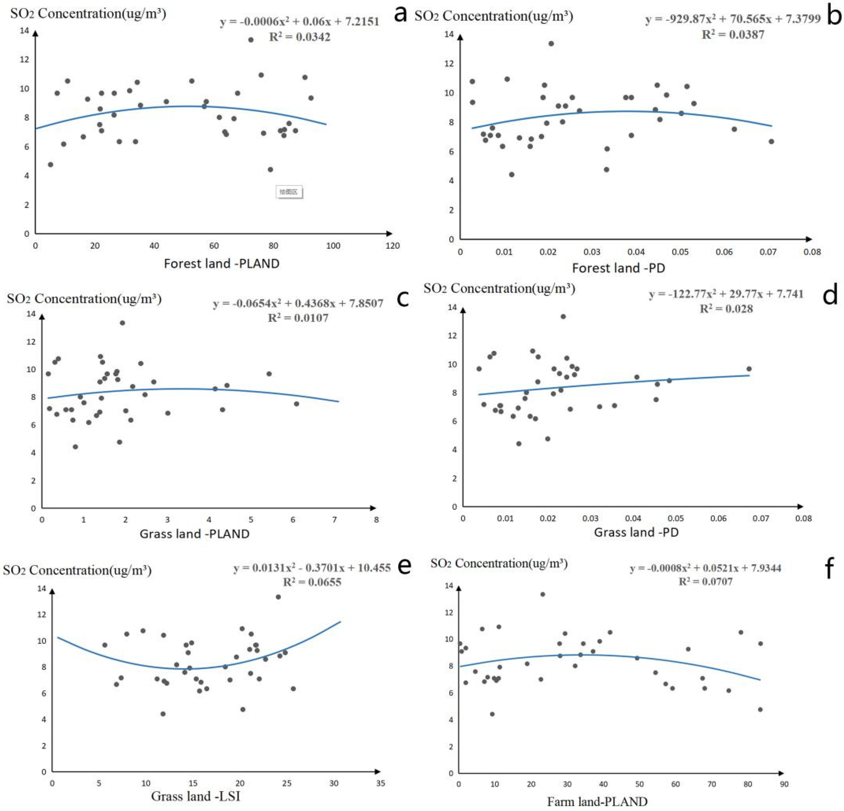
2.1. Regression Analysis of Landscape Pattern Indices and Air Pollutants
2.2. Threshold Effect of the Impact of Landscape Pattern Indices on Air Quality
2.2.1. Threshold Effect of the Impact of Landscape Pattern Indices on PM2.5
2.2.2. Threshold Effect of the Impact of Landscape Pattern Indices on NO2
2.2.3. Threshold Effect of the Impact of Landscape Pattern Indices on SO2
3. Discussions
3.1. Impact Mechanism of Landscape Pattern Index on Air Pollutant Concentration
3.1.1. Impact Mechanism of Landscape Pattern Index on PM2.5
3.1.2. Impact Mechanism of Landscape Pattern Index on NO2
3.1.3. Impact Mechanism of Landscape Pattern Index on SO2
3.2. Threshold Mechanism of Landscape Pattern Index on Air Pollutant Concentration
3.2.1. Threshold Effect of PM2.5
3.2.2. Threshold Effect of NO2
3.2.3. Threshold Effect of SO2
3.3. Implications for Urban Planning and Management Policies
3.4. Research Innovations and Limitations
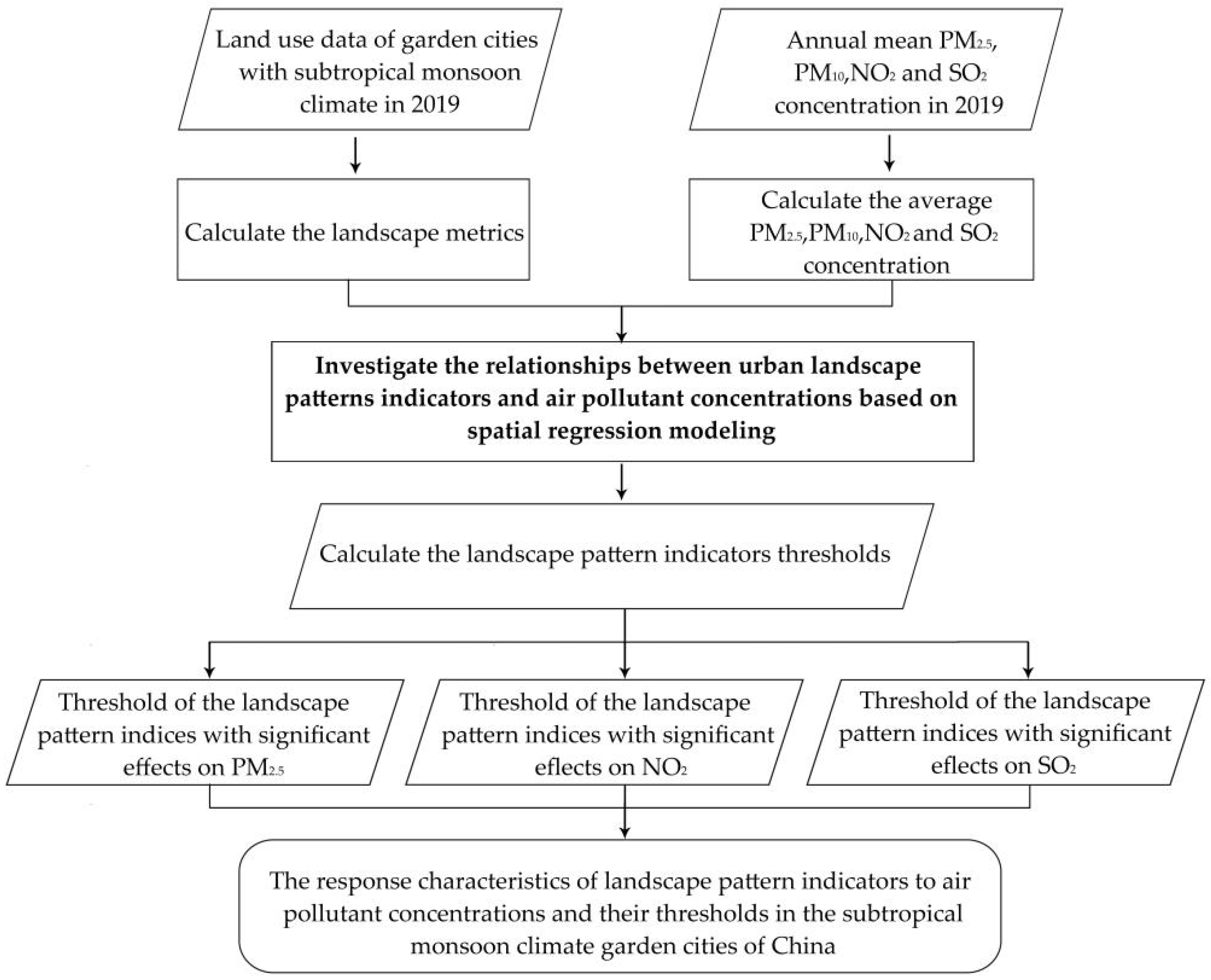
4. Materials and Methods
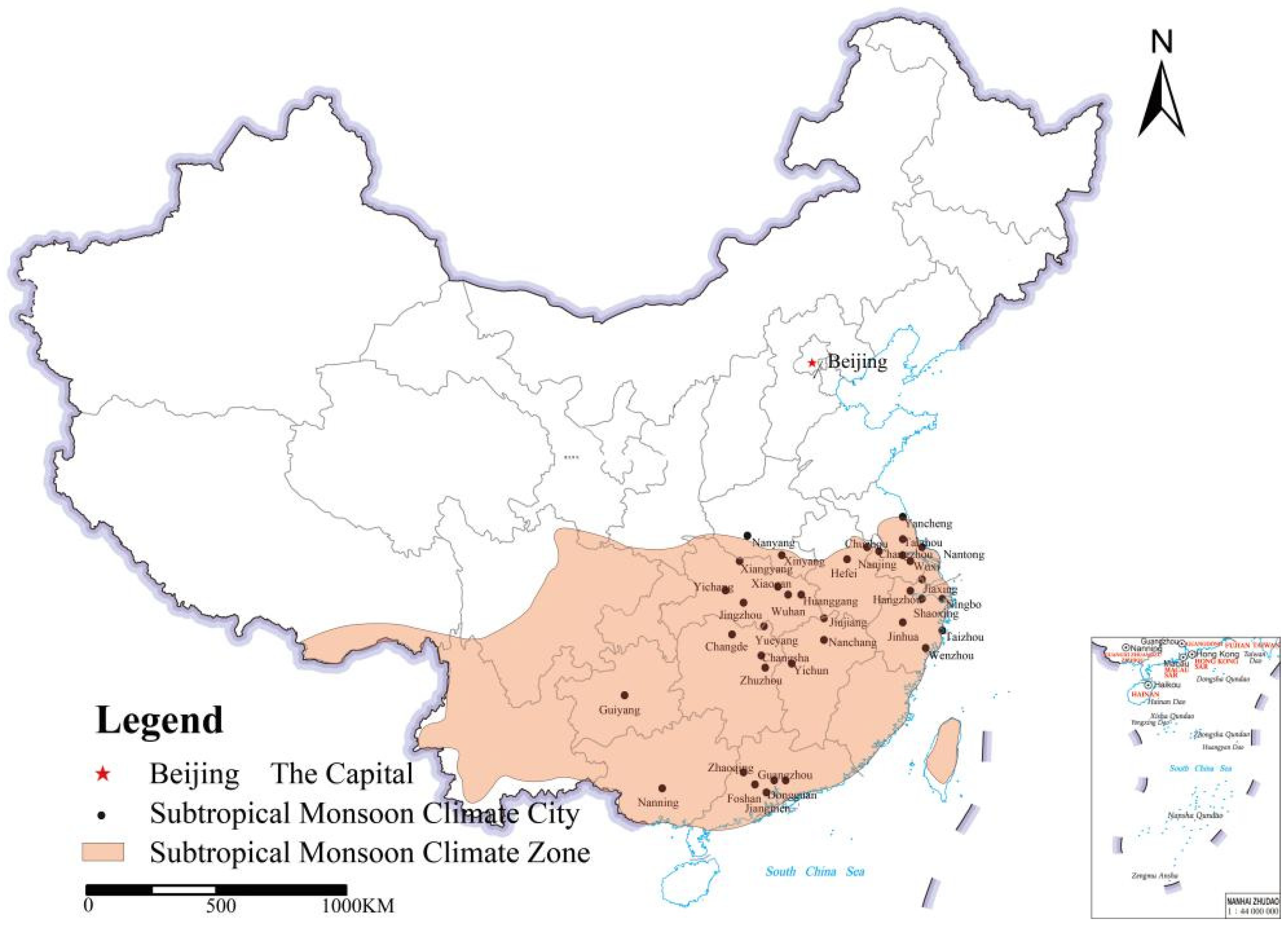
4.1. Study Region
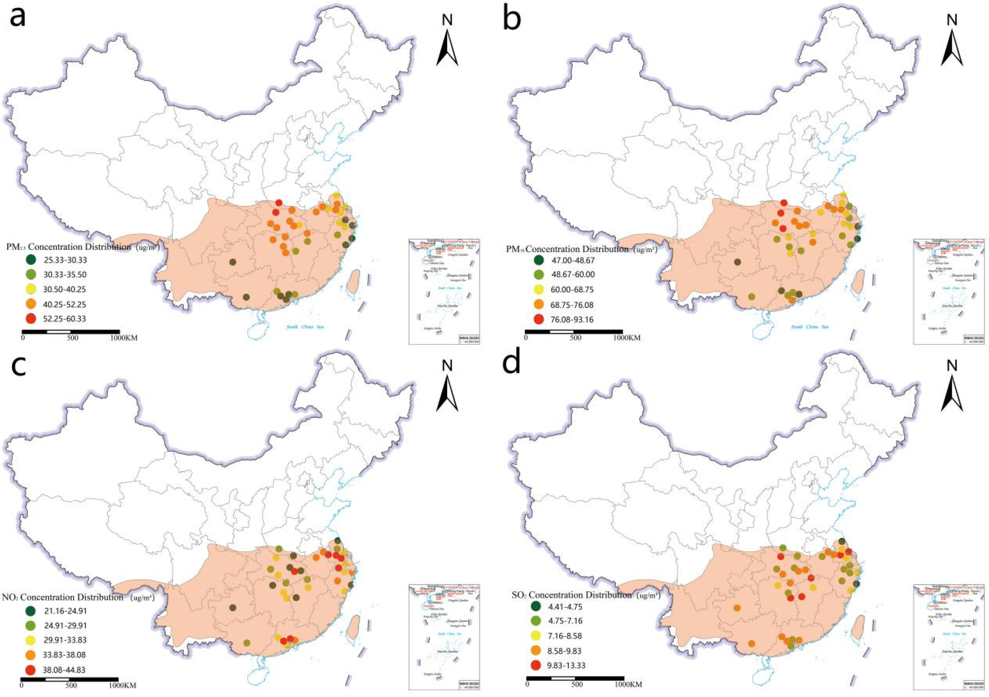
4.2. Data Sources
4.3. Landscape Pattern Indices
4.4. Spatial Regression Modeling Methods
5. Conclusions
- (1)
- The landscape pattern of urban green space was significantly correlated with the concentrations of PM2.5, NO2, and SO2 pollutants in the air, while the concentrations of PM10 pollutants were not significantly affected by the green space pattern.
- (2)
- Among them, the patch shape index (LSI), patch density (PD), and patch proportion in landscape area (PLAND) of forest land can affect the concentration of PM2.5, NO2 and SO2, respectively. The PLAND, PD, and LSI of grassland and farmland can also have an additional impact on the concentration of SO2 pollutants.
- (3)
- The study also found that there was a significant threshold effect on the impact mechanism of urban green space landscape pattern indicators (LSI, PD, PLAND) on the concentrations of PM2.5, NO2, and SO2 air pollutants. When the PD value of forest land is about 0.072, the overall value of urban NO2 pollutant concentration reaches the optimum. When the land and PD values of forest land are away from 50% and 0.038, the land and PD values of grassland are away from 3.33% and 0.121, and the LSI of grassland reaches 14.13, the urban SO2 pollutant concentration reduction effect is the best.
Author Contributions
Funding
Data Availability Statement
Conflicts of Interest
Appendix A

| Greening Indicators | Air Quality Indicators | Social Indicators | |||||
| Serial Number | Name | Greening Rate | PM2.5 (μg/m3) | PM10 (μg/m3) | NO2 (μg/m3) | SO2 (μg/m3) | Population Ten Thousand |
| 1 | Guiyang | 38.20 | 26.66 | 47.00 | 21.16 | 9.66 | 497.14 |
| 2 | Taizhou | 38.20 | 26.66 | 48.67 | 21.66 | 4.41 | 614.00 |
| 3 | Nanning | 34.08 | 30.33 | 52.75 | 29.33 | 9.08 | 734.48 |
| 4 | Ningbo | 37.87 | 28.50 | 47.33 | 35.50 | 7.91 | 854.20 |
| 5 | Wenzhou | 34.49 | 28.00 | 52.92 | 33.83 | 7.58 | 930.00 |
| 6 | Jiangmen | 41.62 | 26.66 | 73.83 | 32.08 | 7.00 | 463.03 |
| 7 | Zhaoqing | 37.99 | 31.75 | 48.00 | 33.50 | 9.33 | 415.17 |
| 8 | Jinhua | 38.15 | 32.41 | 54.4 | 34.41 | 7.16 | 562.40 |
| 9 | Yichun | 44.65 | 35.42 | 59.41 | 23.75 | 13.33 | 558.26 |
| 10 | Yancheng | 39.10 | 39.50 | 66.08 | 24.00 | 4.75 | 720.89 |
| 11 | Jiaxing | 36.15 | 25.33 | 56.25 | 32.75 | 6.66 | 480.00 |
| 12 | Nantong | 40.00 | 36.66 | 55.00 | 31.58 | 10.50 | 731.80 |
| 13 | Dongguan | 37.50 | 31.91 | 48.42 | 36.58 | 9.66 | 846.45 |
| 14 | Shaoxing | 37.19 | 38.00 | 61.58 | 31.58 | 6.91 | 505.70 |
| 15 | Foshan | 42.50 | 29.75 | 56.16 | 41.08 | 9.08 | 815.86 |
| 16 | Nanchang | 38.51 | 35.5 | 69.33 | 33.50 | 8.58 | 560.05 |
| 17 | Guangzhou | 39.91 | 30.00 | 52.66 | 44.83 | 6.83 | 1530.59 |
| 18 | Changde | 39.31 | 47.66 | 60.00 | 22.66 | 8.00 | 577.13 |
| 19 | Xiaogan | unavailable | 43.33 | 72.25 | 21.25 | 7.08 | 492.10 |
| 20 | Huanggang | unavailable | 40.25 | 73.08 | 24.91 | 9.66 | 633.30 |
| 21 | Jiujiang | 44.75 | 45.92 | 63.50 | 29.91 | 10.91 | 492.03 |
| 22 | Yueyang | 39.41 | 43.5 | 67.83 | 26.75 | 8.75 | 577.13 |
| 23 | Taizhou | 38.6 | 43.92 | 67.08 | 28.00 | 7.50 | 463.61 |
| 24 | Changsha | 35.25 | 47.08 | 57.41 | 33.08 | 7.08 | 839.45 |
| 25 | Xinyang | 38.00 | 48.25 | 76.08 | 23.91 | 6.33 | 646.00 |
| 26 | Hangzhou | 37.23 | 37.91 | 66.41 | 41.25 | 6.75 | 1036.00 |
| 27 | Zhuzhou | 34.91 | 47.25 | 65.25 | 33.33 | 10.75 | 402.85 |
| 28 | Yichang | 36.10 | 52.25 | 72.83 | 29.16 | 7.08 | 413.79 |
| 29 | Wuxi | 39.84 | 39.00 | 68.75 | 39.91 | 8.16 | 659.15 |
| 30 | Hefei | 39.75 | 43.58 | 65.75 | 38.08 | 6.16 | 818.90 |
| 31 | Nannjing | 41.00 | 39.75 | 69.16 | 41.75 | 9.83 | 850.00 |
| 32 | Jingzhou | 33.10 | 46.50 | 83.00 | 32.08 | 9.25 | 557.01 |
| 33 | Chuzhou | 42.86 | 48.25 | 72.08 | 35.08 | 9.66 | 414.70 |
| 34 | Changzhou | 39.20 | 46.83 | 71.00 | 41.00 | 10.41 | 473.60 |
| 35 | WUhan | 34.47 | 45.25 | 70.75 | 44.16 | 8.83 | 1121.20 |
| 36 | Xiangyang | 33.34 | 60.33 | 84.58 | 31.58 | 10.50 | 568.00 |
| 37 | Nanyang | 38.10 | 59.66 | 93.16 | 28.83 | 6.33 | 1003.00 |
Appendix B
| Number | City | Forest-PL | Forest-PD | Forest-LSI | Grass-PL | Grass-PD | Grass-LSI | Water-PL | Water-PD | Water-LSI | Farm-PL | Farm-PD | Farm-LSI | Construction-PL | Construction-PD | Construction-LSI |
| 1 | Guiyang | 67.91 | 0.02 | 14.36 | 0.15 | 0.00 | 5.62 | 0.45 | 0.00 | 3.86 | 27.90 | 0.03 | 18.40 | 3.57 | 0.00 | 7.29 |
| 2 | Taizhou | 78.94 | 0.01 | 13.00 | 0.80 | 0.01 | 11.81 | 2.54 | 0.01 | 10.71 | 9.30 | 0.04 | 23.85 | 8.36 | 0.02 | 13.31 |
| 3 | Nanning | 57.40 | 0.02 | 23.86 | 1.39 | 0.02 | 24.82 | 1.11 | 0.01 | 11.88 | 37.16 | 0.02 | 27.25 | 2.94 | 0.01 | 15.06 |
| 4 | Ningbo | 66.70 | 0.02 | 14.07 | 1.42 | 0.02 | 14.65 | 3.21 | 0.01 | 12.45 | 11.36 | 0.038 | 20.95 | 17.22 | 0.02 | 12.41 |
| 5 | Wenzhou | 85.19 | 0.01 | 8.59 | 1.00 | 0.01 | 14.13 | 1.60 | 0.01 | 10.37 | 4.62 | 0.02 | 18.27 | 7.50 | 0.01 | 10.79 |
| 6 | Jiangmen | 63.61 | 0.02 | 19.43 | 2.01 | 0.03 | 18.94 | 5.43 | 0.02 | 14 | 22.74 | 0.02 | 22.09 | 6.04 | 0.01 | 10.31 |
| 7 | Zhaoqing | 92.56 | 0.00 | 7.93 | 1.50 | 0.02 | 21.04 | 2.17 | 0.01 | 12.42 | 1.98 | 0.01 | 13.48 | 1.77 | 0.01 | 11.32 |
| 8 | Jinhua | 83.64 | 0.01 | 12.86 | 0.18 | 0.01 | 7.35 | 0.32 | 0.00 | 7.18 | 8.01 | 0.03 | 21.79 | 7.83 | 0.02 | 17.34 |
| 9 | Yichun | 72.37 | 0.02 | 18.35 | 1.93 | 0.02 | 24.09 | 0.83 | 0.01 | 12.24 | 23.26 | 0.02 | 24.02 | 1.60 | 0.01 | 11.61 |
| 10 | Yancheng | 5.12 | 0.03 | 27.57 | 1.86 | 0.02 | 20.31 | 5.84 | 0.01 | 10.80 | 83.39 | 0.00 | 8.80 | 3.53 | 0.01 | 11.79 |
| 11 | Jiaxing | 16.13 | 0.07 | 23.68 | 1.31 | 0.01 | 6.85 | 4.45 | 0.01 | 9.24 | 57.23 | 0.01 | 11.89 | 20.87 | 0.03 | 12.25 |
| 12 | Nantong | 10.85 | 0.04 | 24.88 | 0.31 | 0.01 | 7.95 | 1.83 | 0.00 | 5.64 | 78.03 | 0.01 | 9.15 | 8.92 | 0.01 | 10.51 |
| 13 | Dongguan | 26.50 | 0.04 | 11.61 | 5.43 | 0.07 | 14.27 | 4.42 | 0.03 | 9.57 | 0.38 | 0.01 | 4.45 | 62.62 | 0.01 | 6.71 |
| 14 | Shaoxing | 76.63 | 0.01 | 12.29 | 1.38 | 0.01 | 11.92 | 0.89 | 0.01 | 8.48 | 10.43 | 0.03 | 18.52 | 10.66 | 0.02 | 12.65 |
| 15 | Foshan | 44.00 | 0.02 | 13.59 | 2.68 | 0.04 | 14.49 | 8.07 | 0.03 | 14.02 | 0.83 | 0.01 | 5.38 | 42.85 | 0.02 | 9.32 |
| 16 | Nanchang | 21.78 | 0.05 | 22.99 | 4.14 | 0.05 | 22.72 | 17.85 | 0.02 | 11.95 | 49.34 | 0.01 | 16.50 | 6.79 | 0.01 | 7.06 |
| 17 | Guangzhou | 64.12 | 0.02 | 15.59 | 3.01 | 0.03 | 15.85 | 2.08 | 0.02 | 13.69 | 7.11 | 0.03 | 17.65 | 23.47 | 0.01 | 11.66 |
| 18 | Changde | 61.78 | 0.02 | 22.29 | 0.92 | 0.01 | 18.44 | 4.00 | 0.01 | 17.97 | 32.21 | 0.01 | 24.54 | 1.08 | 0.00 | 8.46 |
| 19 | Xiaogan | 22.24 | 0.04 | 22.67 | 4.32 | 0.04 | 22.05 | 3.58 | 0.01 | 8.97 | 67.43 | 0.01 | 14.38 | 2.43 | 0.01 | 8.29 |
| 20 | Huanggang | 22.24 | 0.04 | 22.67 | 1.56 | 0.02 | 21.73 | 4.92 | 0.01 | 16.62 | 34.45 | 0.02 | 28.23 | 2.35 | 0.01 | 11.59 |
| 21 | Jiujiang | 75.83 | 0.01 | 14.01 | 1.40 | 0.02 | 20.23 | 9.90 | 0.00 | 11.38 | 11.13 | 0.02 | 21.65 | 1.66 | 0.01 | 10.75 |
| 22 | Yueyang | 56.73 | 0.03 | 19.11 | 2.17 | 0.02 | 19.63 | 11.53 | 0.01 | 13.25 | 28.05 | 0.017 | 23.50 | 1.48 | 0.00 | 7.71 |
| 23 | Taizhou | 21.62 | 0.06 | 24.27 | 6.09 | 0.05 | 21.13 | 7.02 | 0.01 | 10.55 | 54.43 | 0.018 | 13.40 | 10.76 | 0.015 | 10.47 |
| 24 | Changsha | 82.30 | 0.01 | 12.73 | 0.71 | 0.01 | 11.18 | 0.63 | 0.00 | 7.58 | 11.05 | 0.03 | 23.63 | 5.29 | 0.01 | 8.13 |
| 25 | Xinyang | 28.20 | 0.02 | 13.88 | 0.74 | 0.01 | 16.47 | 1.54 | 0.01 | 10.94 | 68.01 | 0.01 | 9.65 | 1.50 | 0.01 | 9.47 |
| 26 | Hangzhou | 83.47 | 0.01 | 9.68 | 0.36 | 0.01 | 12.21 | 3.81 | 0.00 | 11.94 | 1.97 | 0.01 | 16.25 | 10.36 | 0.01 | 11.57 |
| 27 | Zhuzhou | 90.53 | 0.00 | 8.78 | 0.39 | 0.01 | 9.68 | 0.66 | 0.00 | 8.50 | 6.51 | 0.02 | 18.69 | 1.90 | 0.00 | 7.06 |
| 28 | Yichang | 87.35 | 0.01 | 7.36 | 0.57 | 0.01 | 15.34 | 1.21 | 0.00 | 12.80 | 9.81 | 0.00 | 12.80 | 1.03 | 0.00 | 8.33 |
| 29 | Wuxi | 26.43 | 0.05 | 21.93 | 2.47 | 0.02 | 13.26 | 19.74 | 0.01 | 5.33 | 18.94 | 0.03 | 16.54 | 32.39 | 0.02 | 10.37 |
| 30 | Hefei | 9.52 | 0.03 | 21.98 | 1.12 | 0.02 | 15.70 | 8.41 | 0.01 | 5.91 | 74.66 | 0.01 | 10.69 | 6.28 | 0.01 | 7.56 |
| 31 | Nannjing | 31.67 | 0.05 | 27.87 | 1.79 | 0.03 | 14.853 | 10.58 | 0.01 | 8.36 | 38.99 | 0.03 | 21.35 | 16.85 | 0.02 | 9.40 |
| 32 | Jingzhou | 17.56 | 0.05 | 33.33 | 1.81 | 0.03 | 21.83 | 14.92 | 0.01 | 16.36 | 63.47 | 0.01 | 16.36 | 2.21 | 0.01 | 9.52 |
| 33 | Chuzhou | 7.35 | 0.03 | 19.66 | 1.77 | 0.03 | 21.67 | 4.80 | 0.01 | 13.71 | 83.47 | 0.00 | 11.46 | 2.59 | 0.01 | 10.91 |
| 34 | Changzhou | 34.23 | 0.05 | 23.64 | 2.37 | 0.02 | 11.87 | 9.09 | 0.01 | 6.11 | 29.42 | 0.03 | 18.12 | 24.88 | 0.02 | 8.55 |
| 35 | Wuhan | 35.31 | 0.04 | 32.20 | 4.43 | 0.05 | 24.25 | 15.11 | 0.02 | 16.60 | 33.69 | 0.032 | 24.62 | 11.29 | 0.01 | 10.32 |
| 36 | Xiangyang | 52.55 | 0.02 | 12.00 | 1.45 | 0.02 | 21.20 | 1.23 | 0.01 | 12.96 | 41.86 | 0.01 | 14.72 | 2.90 | 0.01 | 17.15 |
| 37 | Nanyang | 33.64 | 0.01 | 12.49 | 2.13 | 0.02 | 25.68 | 1.52 | 0.00 | 6.34 | 59.12 | 0.01 | 15.14 | 3.57 | 0.025 | 28.08 |
References
- Gianfredi, V.; Buffoli, M.; Rebecchi, A.; Croci, R.; Oradini-Alacreu, A.; Stirparo, G.; Marino, A.; Odone, A.; Capolongo, S.; Signorelli, C. Association between Urban Greenspace and Health: A Systematic Review of Literature. Int. J. Environ. Res. Public Health 2021, 18, 5137. [Google Scholar] [CrossRef] [PubMed]
- Reyes-Riveros, R.; Altamirano, A.; De La Barrera, F.; Rozas-Vásquez, D.; Vieli, L.; Meli, P. Linking public urban green spaces and human well-being: A systematic review. Urban For. Urban Green. 2021, 61, 127105. [Google Scholar] [CrossRef]
- Barrett, E.; Apodaca, K. Response to “Alcohol and COVID-19: How Do We Respond to This Growing Public Health Crisis?”. J. Gen. Intern. Med. 2021, 36, 2476. [Google Scholar] [CrossRef] [PubMed]
- Jaafari, S.; Shabani, A.A.; Moeinaddini, M.; Danehkar, A.; Sakieh, Y. Applying landscape metrics and structural equation modeling to predict the effect of urban green space on air pollution and respiratory mortality in Tehran. Environ. Monit. Assess. 2020, 192, 412. [Google Scholar] [CrossRef] [PubMed]
- Kim, S.Y.; Kim, S.H.; Wee, J.H.; Min, C.; Han, S.M.; Kim, S.; Choi, H.G. Short and long term exposure to air pollution increases the risk of ischemic heart disease. Sci. Rep. 2021, 11, 51085. [Google Scholar]
- Luo, J.; Niu, Y.; Zhang, Y.; Zhang, M.; Tian, Y.; Zhou, X. Dynamic analysis of retention PM2.5 by plant leaves in rainfall weather conditions of six tree species. Energy Sources Part A Recovery Util. Environ. Eff. 2020, 42, 1014–1025. [Google Scholar] [CrossRef]
- Cai, L.; Zhuang, M.; Ren, Y. A landscape scale study in Southeast China investigating the effects of varied green space types on atmospheric PM2.5 in mid-winter. Urban For. Urban Green. 2020, 49, 126607. [Google Scholar] [CrossRef]
- Latha, K.M.; Highwood, E. Studies on particulate matter (PM10) and its precursors over urban environment of Reading, UK. J. Quant. Spectrosc. Radiat. Transf. 2006, 101, 367–379. [Google Scholar] [CrossRef]
- Beckett, K.P.; Freer-Smith, P.H.; Taylor, G. Urban woodlands: Their role in reducing the effects of particulate pollution. Environ. Pollut. 1998, 99, 347–360. [Google Scholar] [CrossRef]
- Sheng, Q.; Zhu, Z. Physiological Response of European Hornbeam Leaves to Nitrogen Dioxide Stress and Self-recovery. J. Am. Soc. Hortic. Sci. 2019, 144, 23–30. [Google Scholar] [CrossRef] [Green Version]
- Thomas, M.D.; Hill, G.R., Jr. Absorption of sulphur dioxide by alfalfa and its relation to leaf injury. Plant Physiol. 1935, 10, 291. [Google Scholar] [CrossRef] [PubMed]
- Wang, H.; Sun, Y.-Q.; Zhang, M.; Liu, W.J.; Yang, L.; Zhou, X.W. Adsorption ability of air pollutants by indigenous tree species in ta-pieh mountains. Fresenius Environ. Bull. 2019, 28, 2908–2915. [Google Scholar]
- Wang, S.; Li, M. Study on the Principle of Urban Open Space Ecological Planning. Chin. Landsc. Arch. 2001, 5, 33–37. [Google Scholar]
- Sheng, Q.; Zhang, Y.; Zhu, Z.; Li, W.; Xu, J.; Tang, R. An experimental study to quantify road greenbelts and their association with PM2.5 concentration along city main roads in Nanjing, China. Sci. Total Environ. 2019, 667, 710–717. [Google Scholar] [CrossRef] [PubMed]
- Fan, S.; Li, X.; Dong, L. Field assessment of the effects of land-cover type and pattern on PM10 and PM2.5 concentrations in a microscale environment. Environ. Sci. Pollut. Res. 2019, 26, 2314–2327. [Google Scholar] [CrossRef] [PubMed]
- Ye, L.; Fang, L.; Tan, W.; Wang, Y.; Huang, Y. Exploring the effects of landscape structure on aerosol optical depth (AOD) patterns using GIS and HJ-1B images. Environ. Sci. Process. Impacts 2016, 18, 265–276. [Google Scholar] [CrossRef]
- Yue, F.; Dai, F.; Guo, X. Study on Correlation Between Air Pollutants and Vegetation Coverage in Wuhan Based on Remote Sensing Inversion. Landsc. Arch. 2019, 26, 76–81. [Google Scholar]
- Lei, Y.; Davies, G.M.; Jin, H.; Tian, G.; Kim, G. Scale-dependent effects of urban greenspace on particulate matter air pollution. Urban For. Urban Green. 2021, 61, 127089. [Google Scholar] [CrossRef]
- Zhao, L.; Li, T.; Przybysz, A.; Guan, Y.; Ji, P.; Ren, B.; Zhu, C. Effect of urban lake wetlands and neighboring urban greenery on air PM10 and PM2.5 mitigation. Build. Environ. 2021, 206, 108291. [Google Scholar] [CrossRef]
- Alam, M.S.; McNabola, A. Exploring the modeling of spatiotemporal variations in ambient air pollution within the land use regression framework: Estimation of PM10 concentrations on a daily basis. J. Air Waste Manag. Assoc. 2015, 65, 628–640. [Google Scholar] [CrossRef]
- Zhang, H.; Zhao, Y. Land use regression for spatial distribution of urban particulate matter (PM10) and sulfur dioxide (SO2) in a heavily polluted city in Northeast China. Environ. Monit. Assess. 2019, 191, 712. [Google Scholar] [CrossRef] [PubMed]
- Lee, H.J.; Koutrakis, P. Daily ambient NO2 concentration predictions using satellite ozone monitoring instrument NO2 data and land use regression. Environ. Sci. Technol. 2014, 48, 2305–2311. [Google Scholar] [PubMed]
- Lu, D.; Xu, J.; Yue, W.; Mao, W.; Yang, D.; Wang, J. Response of PM2.5 pollution to land use in China. J. Clean. Prod. 2019, 244, 118741. [Google Scholar] [CrossRef]
- de Jalón, S.G.; Burgess, P.; Yuste, J.C.; Moreno, G.; Graves, A.; Palma, J.; Crous-Duran, J.; Kay, S.; Chiabai, A. Dry deposition of air pollutants on trees at regional scale: A case study in the Basque Country. Agric. For. Meteorol. 2019, 278, 107648. [Google Scholar] [CrossRef]
- Anselin, L. Local Indicators of Spatial Association—LISA. Geogr. Anal. 1995, 27, 93–115. [Google Scholar] [CrossRef]
- Getis, A.; Ord, J.K. The Analysis of Spatial Association by Use of Distance Statistics. Geogr. Anal. 2010, 24, 189–206. [Google Scholar] [CrossRef]
- Alastuey, A.; Querol, X.; Plana, F.; Viana, M.; Ruiz, C.R.; De La Campa, A.S.; De La Rosa, J.; Mantilla, E.; Dos Santos, S.G. Identification and chemical characterization of industrial particulate matter sources in southwest Spain. J. Air Waste Manag. Assoc. 2006, 56, 993–1006. [Google Scholar] [CrossRef] [Green Version]
- Chen, L.; Liu, C.; Zhang, L.; Zou, R.; Zhang, Z. Variation in Tree Species Ability to Capture and Retain Airborne Fine Particulate Matter (PM2.5). Sci. Rep. 2017, 7, 3206. [Google Scholar] [CrossRef] [Green Version]
- Liang, D.; Ma, C.; Wang, Y.-Q.; Wang, Y.-J.; Chen-Xi, Z. Quantifying PM2.5 capture capability of greening trees based on leaf factors analyzing. Environ. Sci. Pollut. Res. 2016, 23, 21176–21186. [Google Scholar] [CrossRef] [Green Version]
- Gasmi, K.; Aljalal, A.; Al-basheer, W.; Abdulahi, M. Analysis of NOx, NO and NO2 ambient levels as a function of meteorological parameters in Dhahran, Saudi Arabia. WIT Trans. Ecol. Environ. 2017, 211, 77–86. [Google Scholar]
- Morikawa, H.; Erkin, Ö.C. Basic processes in phytoremediation and some applications to air pollution control. Chemosphere 2003, 52, 1553–1558. [Google Scholar] [CrossRef]
- Guo, Z.; Jiang, H.; Chen, J.; Cheng, M.; Wang, B.; Jiang, Z. The relationship between atmospheric SO2 column density and land use in Zhejiang, China. In Proceedings of the 2009 Joint Urban Remote Sensing Event, Shanghai, China, 20–22 May 2009; pp. 1–6. [Google Scholar] [CrossRef]
- Li, C.; Xu, Y.; Liu, M.; Hu, Y.; Huang, N.; Wu, W. Modeling the Impact of Urban Three-Dimensional Expansion on Atmospheric Environmental Conditions in an Old Industrial District: A Case Study in Shenyang, China. Pol. J. Environ. Stud. 2020, 29, 3171–3181. [Google Scholar] [CrossRef]
- Li, Y.; Shi, J. Characteristics of SO2 Dispersion in Urban of Taiyuan‚ Shanxi. J. Shanxi Univ. 2011, 34, 153–157. [Google Scholar]
- Shao, T.; Zhou, Z.; Wang, P.; Tang, W.; Liu, X.; Hu, X. Relationship between urban green-land landscape patterns and air pollution in the central district of Yichang city. Ying Yong Sheng Tai Xue Bao J. Appl. Ecol. 2004, 15, 691–696. [Google Scholar]
- Spedding, D.J. Uptake of Sulphur Dioxide by Barley Leaves at Low Sulphur Dioxide Concentrations. Nature 1969, 224, 1229–1231. [Google Scholar] [CrossRef]
- Li, K.; Li, C.; Liu, M.; Hu, Y.; Wang, H.; Wu, W. Multiscale analysis of the effects of urban green infrastructure landscape patterns on PM2.5 concentrations in an area of rapid urbanization. J. Clean. Prod. 2021, 325, 129324. [Google Scholar] [CrossRef]
- Yang, Y. The effect of urban form on PM2.5 concentration: Evidence from china’s 340 prefecture-level cities. Remote Sens. 2021, 14, 7. [Google Scholar]
- Rao, M.; George, L.A.; Rosenstiel, T.N.; Shandas, V.; Dinno, A. Assessing the relationship among urban trees, nitrogen dioxide, and respiratory health. Environ. Pollut. 2014, 194, 96–104. [Google Scholar] [CrossRef]
- Klingberg, J.; Broberg, M.; Strandberg, B.; Thorsson, P.; Pleijel, H. Influence of urban vegetation on air pollution and noise exposure—A case study in Gothenburg, Sweden. Sci. Total Environ. 2017, 599, 1728–1739. [Google Scholar] [CrossRef]
- Geng, Y.C.; Li, J. The value evaluation on the forest resource of forest industry zone of heilongjiang province in acid rain prevention. In Proceedings of the Asia-Pacific Power and Energy Engineering Conference, Wuhan, China, 25–28 March 2011; IEEE Computer Society: Washington, DC, USA, 2011. [Google Scholar]
- He, Z.; Shi, X.; Wang, X.; Xu, Y. Urbanisation and the geographic concentration of industrial SO2 emissions in China. Urban Stud. 2017, 54, 3579–3596. [Google Scholar] [CrossRef]
- Wickham, J.D.; Jones, K.B.; Riitters, K.H.; O’Neill, R.V.; Tankersley, R.D.; Smith, E.R.; Chaloud, D.J. An integrated environmental assessment of the us mid—Atlantic region. Environ. Manag. 1999, 24, 553–560. [Google Scholar] [CrossRef] [PubMed]
- Rafiee, R.; Mahiny, A.S.; Khorasani, N. Assessment of changes in urban green spaces of Mashad city using satellite data. Int. J. Appl. Earth Obs. Geoinf. 2009, 11, 431–438. [Google Scholar] [CrossRef]
- Wu, J.; Xie, W.; Li, W.; Li, J. Effects of Urban Landscape Pattern on PM2.5 Pollution—A Beijing Case Study. PLoS ONE 2015, 10, e0142449. [Google Scholar] [CrossRef] [PubMed] [Green Version]
- Xu, G.; Jiao, L.; Zhao, S.; Yuan, M.; Li, X.; Han, Y.; Zhang, B.; Dong, T. Examining the Impacts of Land Use on Air Quality from a Spatio-Temporal Perspective in Wuhan, China. Atmosphere 2016, 7, 62. [Google Scholar] [CrossRef] [Green Version]
- Li, C.; Zhang, K.; Dai, Z.; Ma, Z.; Liu, X. Investigation of the impact of land-use distribution on PM2.5 in Weifang: Seasonal variations. Int. J. Environ. Res. Public Health 2020, 17, 5135. [Google Scholar] [CrossRef]
- Garcia-Menendez, F.; Monier, E.; Selin, N.E. The role of natural variability in projections of climate change impacts on U.S. ozone pollution. Geophys. Res. Lett. 2017, 44, 2911–2921. [Google Scholar] [CrossRef] [Green Version]
- Lu, D.; Mao, W.; Yang, D.; Zhao, J.; Xu, J. Effects of land use and landscape pattern on PM2.5 in Yangtze River Delta, China. Atmos. Pollut. Res. 2018, 9, 705–713. [Google Scholar] [CrossRef]
- Xiao, H.; Huang, Z.; Zhang, J.; Zhang, H.; Chen, J.; Zhang, H.; Tong, L. Identifying the impacts of climate on the regional transport of haze pollution and inter-cities correspondence within the Yangtze River Delta. Environ. Pollut. 2017, 228, 26–34. [Google Scholar] [CrossRef]
- Parker, D.C.; Evans, T.; Meretsky, V. Measuring Emergent Properties of Agent-Based Landcover/Landuse Models Using Spatial Metrics; Society for Computational Economics: Dallas, TX, USA, 2001. [Google Scholar]
- Lee, W.J.; Park, C. Prediction of apartment prices per unit in Daegu-Gyeongbuk areas by spatial regression models. J. Korean Data Inf. Sci. Soc. 2015, 26, 561–568. [Google Scholar] [CrossRef] [Green Version]
- Tu, M.; Liu, Z.; He, C.; Fang, Z.; Lu, W. The relationships between urban landscape patterns and fine particulate pollution in China: A multiscale investigation using a geographically weighted regression model. J. Clean. Prod. 2019, 237, 117744. [Google Scholar] [CrossRef]


| Variable | p | Threshold | p | Threshold | p | Threshold | p | Threshold | |
|---|---|---|---|---|---|---|---|---|---|
| PM2.5 | PM10 | NO2 | SO2 | ||||||
| Forest land | PLAND | 0.569 | 0.161 | 0.774 | 0.09 * | 50 | |||
| PD | 0.41 | 0.513 | 0.091 * | 0.0718 | 0.003 *** | 0.038 | |||
| LSI | 0.059 * | 18.018 | 0.323 | 0.204 | 0.493 | ||||
| Grassland | PLAND | 0.847 | 0.764 | 0.816 | 0.031 ** | 3.33 | |||
| PD | 0.571 | 0.751 | 0.9902 | 0.000 *** | 0.121 | ||||
| LSI | 0.182 | 0.499 | 0.818 | 0.000 *** | 14.13 | ||||
| Farm land | PLAND | 0.247 | 0.537 | 0.592 | 0.001 *** | 32.56 | |||
| PD | 0.652 | 0.921 | 0.624 | 0.925 | |||||
| LSI | 0.309 | 0.592 | 0.774 | 0.139 | |||||
| Metrics (Abbreviation) | Calculation Formula | Description |
|---|---|---|
| Percentage of landscape types (PLAND) | PLAND = | PLAND quantifies the proportional abundance of each patch type in the landscape (percent) |
| Patch density (PD) | PD = | PD expresses number of patches on a per unit area for considered class (number per 100 hectares) |
| Landscape shape index (LSI) | LSI = | LSI expresses the larger LSI value is, the more complex landscape shape is. |
| Model | R2 | LogL | AIC | SC | |
|---|---|---|---|---|---|
| PM2.5 | SEM | 0.747 | −116.730 | 265.46 | 291.662 |
| SAR | 0.716 | −116.772 | 267.543 | 295.382 | |
| PM10 | SEM | 0.744 | −123.79 | 279.581 | 305.782 |
| SAR | 0.73 | −122.789 | 279.577 | 307.416 | |
| NO2 | SEM | 0.549 | −108.694 | 249.39 | 275.591 |
| SAR | 0.525 | −111.464 | 256.928 | 284.767 | |
| SO2 | SEM | 0.6339 | −60.004 | 152.01 | 178.211 |
| SAR | 0.41 | −67.446 | 168.894 | 196.733 |
Publisher’s Note: MDPI stays neutral with regard to jurisdictional claims in published maps and institutional affiliations. |
© 2022 by the authors. Licensee MDPI, Basel, Switzerland. This article is an open access article distributed under the terms and conditions of the Creative Commons Attribution (CC BY) license (https://creativecommons.org/licenses/by/4.0/).
Share and Cite
Wang, C.; Guo, M.; Jin, J.; Yang, Y.; Ren, Y.; Wang, Y.; Cao, J. Does the Spatial Pattern of Plants and Green Space Affect Air Pollutant Concentrations? Evidence from 37 Garden Cities in China. Plants 2022, 11, 2847. https://doi.org/10.3390/plants11212847
Wang C, Guo M, Jin J, Yang Y, Ren Y, Wang Y, Cao J. Does the Spatial Pattern of Plants and Green Space Affect Air Pollutant Concentrations? Evidence from 37 Garden Cities in China. Plants. 2022; 11(21):2847. https://doi.org/10.3390/plants11212847
Chicago/Turabian StyleWang, Chengkang, Mengyue Guo, Jun Jin, Yifan Yang, Yujie Ren, Yang Wang, and Jiajie Cao. 2022. "Does the Spatial Pattern of Plants and Green Space Affect Air Pollutant Concentrations? Evidence from 37 Garden Cities in China" Plants 11, no. 21: 2847. https://doi.org/10.3390/plants11212847