Article

Archaeological Predictive Modeling Using Machine Learning and Statistical Methods for Japan and China

1
Graduate School of Frontier Sciences, The University of Tokyo, 5-1-5, Kashiwanoha, Kashiwa 277-8563, Japan
2
School of Business, Society and Technology, Mälardalens University, 72123 Västerås, Sweden
3
Center for Spatial Information Science, The University of Tokyo, 5-1-5, Kashiwanoha, Kashiwa 277-8568, Japan
*
Author to whom correspondence should be addressed.
ISPRS Int. J. Geo-Inf. 2023, 12(6), 238; https://doi.org/10.3390/ijgi12060238
Submission received: 21 April 2023 / Revised: 30 May 2023 / Accepted: 1 June 2023 / Published: 7 June 2023

Abstract

:
Archaeological predictive modeling (APM) is an essential method for quantitatively assessing the probability of archaeological sites present in a region. It is a necessary tool for archaeological research and cultural heritage management. In particular, the predictive modeling process could help us understand the relationship between past human civilizations and the natural environment; moreover, a better understanding of the mechanisms of the human–land relationship can provide new ideas for sustainable development. This study aims to investigate the impact of topographic and hydrological factors on archaeological sites in the Japanese archipelago and Shaanxi Province, China and proposes a hybrid integration approach for APM. This approach employed a conditional attention mechanism (AM) using deep learning and a frequency ratio (FR) model, in addition to a separate FR model and the widely-used machine learning MaxEnt method. The models’ outcomes were cross-checked using the four-fold cross-validation method, and the models’ performances were compared using the area under the receiver operating characteristic curve (AUC) and Kvamme’s Gain. The results showed that in both study areas, the AM_FR model exhibited the most satisfactory performances.

1. Introduction

A basic definition of archaeological predictive modeling (APM) was proposed by Kohler and Parker [1] as “a technique that, at a minimum, tries to predict the locations of archaeological sites or materials in a region, based either on a sample of that region or on fundamental notions concerning human behavior.” With further technological innovations, APM has now become an essential method for quantitatively assessing the probability of archaeological sites’ presence, and has been successfully applied in archaeological research and cultural resource protection in many areas of the world, including northwestern Belize [2], northeastern Romania [3], South Central Utah, USA [4], Israel, and Northeast China [5].
Willey’s [6] pioneering work in Viru Valley, USA, has played an essential role in the history of predictive modeling, influencing the development of subsequent analyses and methods. As the origin of directional settlement research, Willey’s work revealed that the location of human settlements is closely related to the characteristics of the natural environment. Subsequent studies by other scholars [7,8,9,10,11] further elucidated the relationship between archaeological sites and space: the locations of archaeological sites are non-random since spatial conditions limit human behaviors. As such, the realization that archaeological sites are closely related to the natural environment, coupled with the processual emphasis on quantitative methods, enabled the formulation of statistical models for predicting archaeological sites in a region. The input parameters are critical to the results of predictive modeling. Studies by other scholars [12,13,14,15,16] have shown that topographic factors and distance from bodies of water play an important role in the distribution of archaeological sites. However, topographic factors have not received sufficient attention in the existing research. In the current related studies, three or four topographic factors, such as elevation, slope, and curvature, are generally examined; however, these represent only a few topographic characteristics.
Since the APM was first proposed, the research subjects have become increasingly varied, and the research methods have continuously utilized innovative methods. For example, with the recent development of artificial intelligence, some machine learning models have been applied to APM [4,5]. However, as Verhagen and Whitley [17] point out, the predictive model as a cultural resource management (CRM) tool has achieved reasonable success, but it has not commanded much respect from academic scholars. This is due to the desire to use predictive models for minimizing field effort rather than for explaining the differential spatial patterning of archaeological sites. Indeed, much current research focuses on the study of the model itself but overlooks the relationship between archaeological sites and the surrounding natural environments.
In our quest to comprehend the key factors influencing past human landform utilization, we propose a hybrid integration approach for APM with a conditional deep learning attention mechanism (AM) and a frequency ratio (FR). This method intends to tackle the limitation that FR is a density transfer and is unable to accurately decide the importance of individual factors [18]. Furthermore, the original FR model and the MaxEnt method [4,5] were applied to the same data for comparison. Eight predictive input factors were selected for this study. These included elevation, slope, and distance from a river, which are commonly used, as well as several topographical factors rarely used in APM: roughness, relief degree of the land surface (RDLS), plan curvature, profile curvature, and cutting depth. Our proposed data-driven deep learning AM can model these inputs jointly to analyze how they interact with the locations of archaeological sites. In this process, the model learns the effect of all input factors on archaeological site locations and then automatically selects the most relevant factors under the class labels of archaeological sites. We focus on the model’s performance and the relationship between archaeological sites and environmental factors and offer explanations for the model’s results. This can help us understand the relationship between past human civilizations and the natural environment.

2. Materials

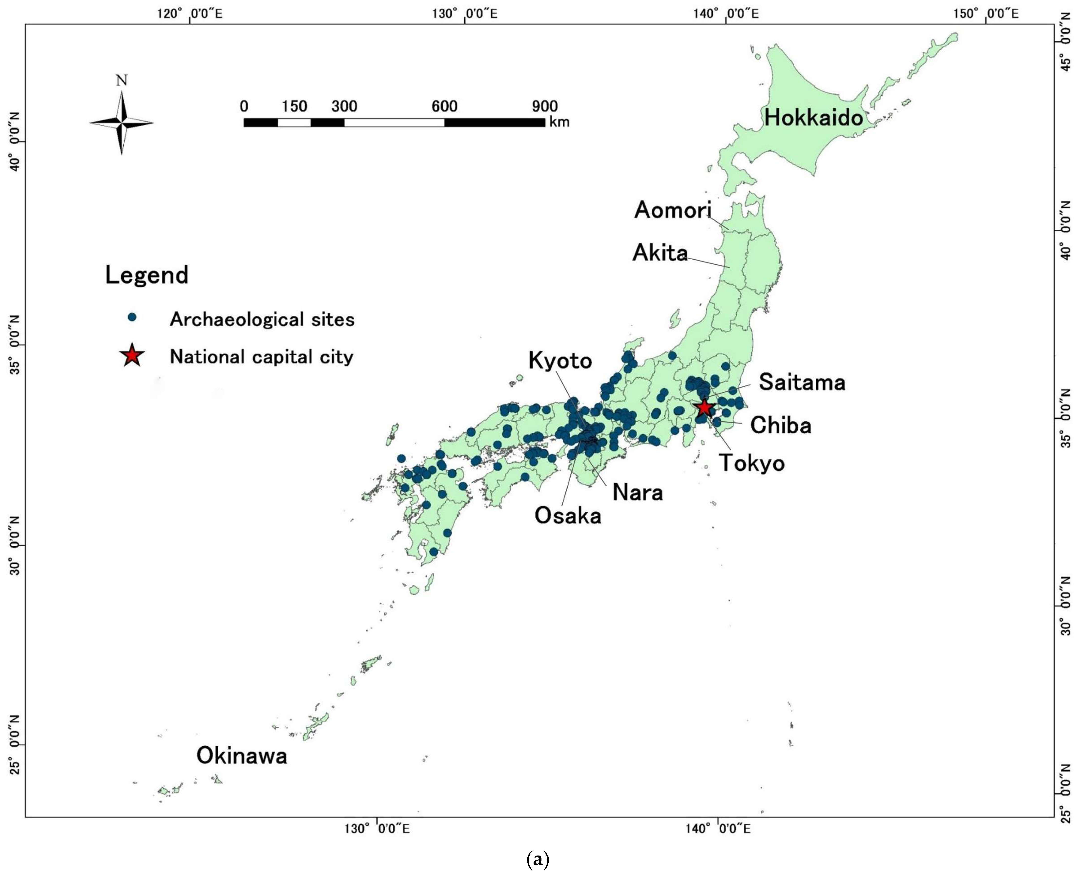
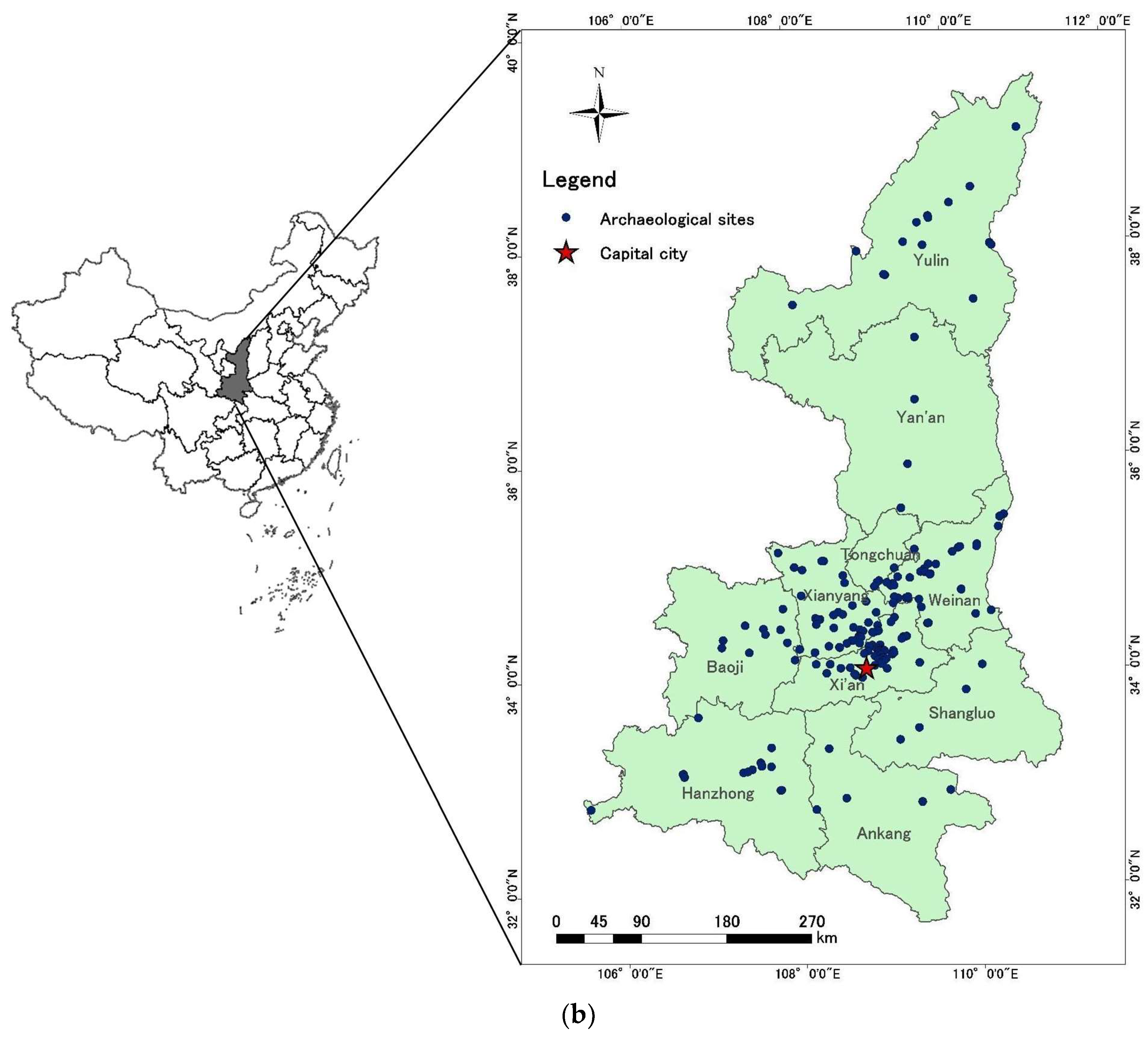
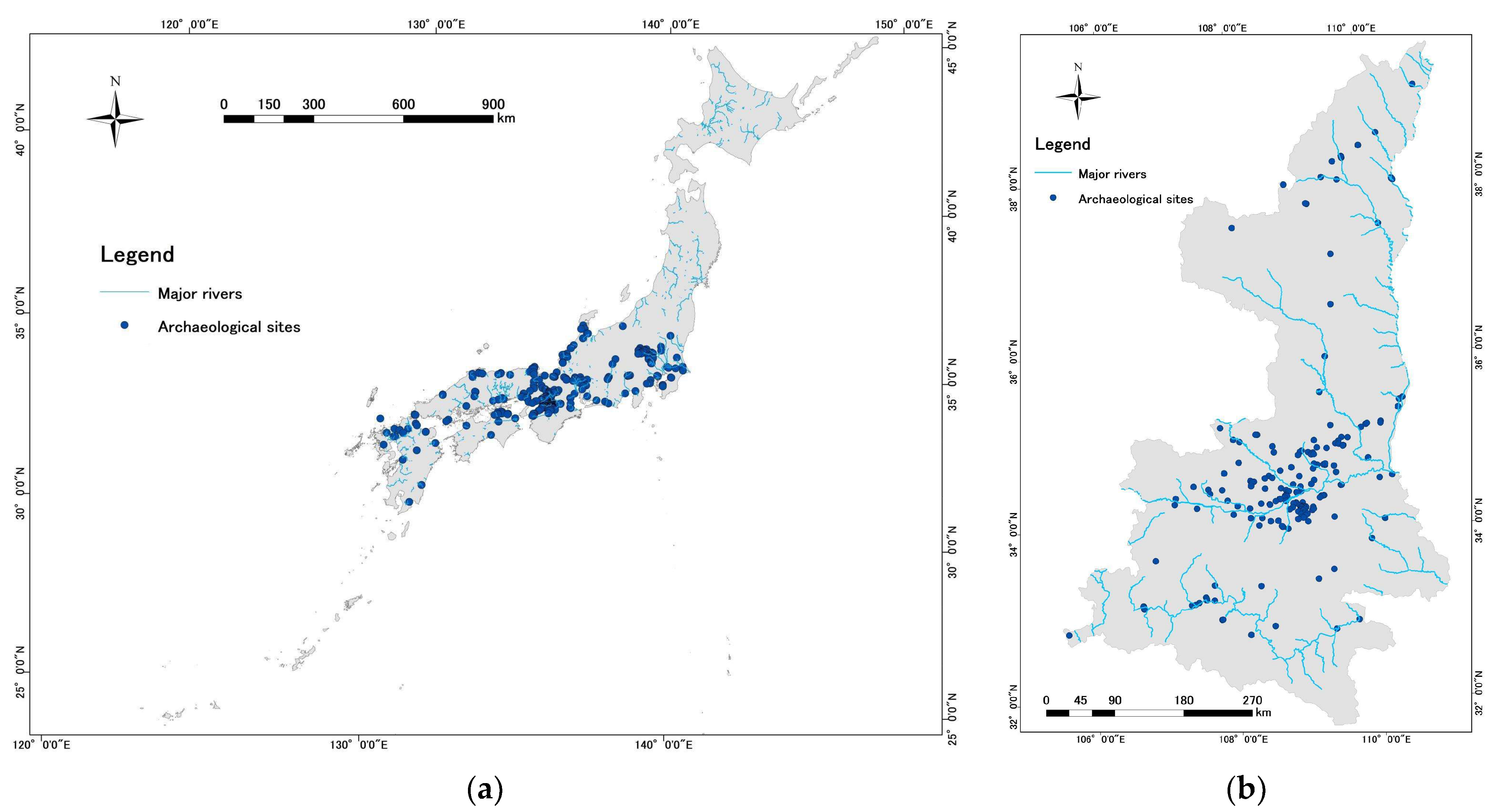
2.1. Study Area and Archaeological Background

The study explored the Japanese archipelago (Figure 1a) and Shaanxi Province, China (Figure 1b). These areas were selected because they represent two distinct topographies along an island arc and in a continent, which may affect the interactions between archaeological sites and topographic factors, as well as water availability. The analysis of such areas may provide insight into how past humans interacted with the natural environment under different environmental conditions.
Japan is an island country in East Asia located around the northwest Pacific Ocean, with 6852 islands covering 377,975 km2. Approximately three-quarters of the country’s terrain is mountainous [19]. Kyoto and Nara are representative historical capitals, home to thousands of archaeological sites (monuments, rituals, burial sites, etc.) [20]. The Japanese archaeological sites considered in this study are burial tombs built in the Kofun period, from the 3rd to the 6th centuries CE [21] or between the middle of the 3rd and the early 7th centuries [22]. The Kofun era is named for the large earthen tombs that characterized and defined the period. The typical tomb type is called “Zempō-kōen fun” in Japanese from its characteristic shape: a square protrusion connects to a main circular hill, forming a keyhole shape [22,23]. Hence, the name “Keyhole-shaped tomb” is used in some related studies [24,25]. The scale of the tombs ranges from several meters to more than 400 m [26,27,28]; the tomb’s size is thought to represent the buried person’s power and status [29,30]. In addition, this keyhole-shaped tomb is unique to Japan [31].
Shaanxi Province is an inland region located in Northwest China; it has a total area of 205,800 km2. Approximately 45% of the area consists of plateaus, followed by mountains (36%) and plains (18%) [31]. The province is an important cradleland of the Chinese nation. For nearly 2000 years, from the establishment of the Western Zhou Dynasty to the fall of the Tang Dynasty, 14 successive dynasties established their capitals there [32]. Particularly notable is Xi’an, the current capital city of the province with a long and rich cultural history, where most previous dynasties established their capitals [33]. Moreover, the Silk Road, the historical network of Eurasian trade routes, originated in this region [34]. The Mausoleum of Qin Shihuang in Shaanxi Province is the largest tomb in Chinese history. Xi’an also has the Terracotta Warriors and Horses in a mausoleum, China’s earliest World Heritage Site. There are many ground-level and underground ruins near the mausoleum [35]. Because of its diverse cultural history, the Shaanxi dataset contains a variety of archaeological monuments, such as tombs, temples, and palaces, spanning over 2000 years (1046 BC–907 AD).

2.2. Archaeological Data

The archaeological site data included archaeological or historical monuments and tombs in Japan (n = 1367) and Shaanxi, China (n = 200) (for details, see supplementary). For Japan, these data were collected from an open-access database named the Kofun database, compiled by researchers at Osaka Electro-Communication University. This database lists specific attributes of the archaeological sites, including location, direction, and construction time. For China, the archaeological site data were collected from the Chinese Archaeology website provided by the Institute of Archaeology, the Chinese Academy of Sciences. Initially, archaeological site data from the mentioned publication and database could not be input directly into the ArcGIS 10.6 platform, as the data did not include geographical coordinates. To this end, we vectorized the archaeological sites and stored them in the digital geographic database as point data (Figure 1); these points are mainly located in the centers of the archaeological sites. The same amount of absence data was randomly generated under a restriction of 10 km outward from the archaeological sites.

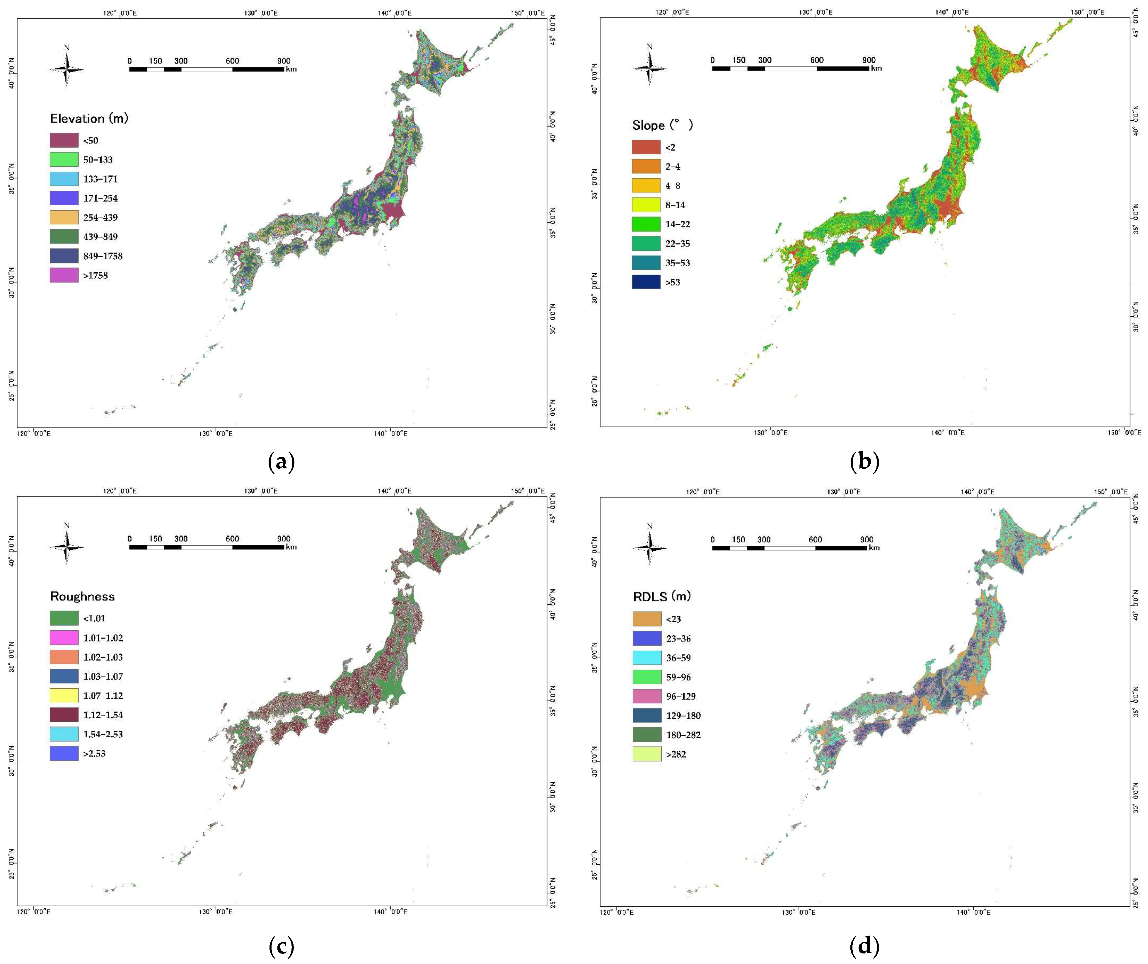
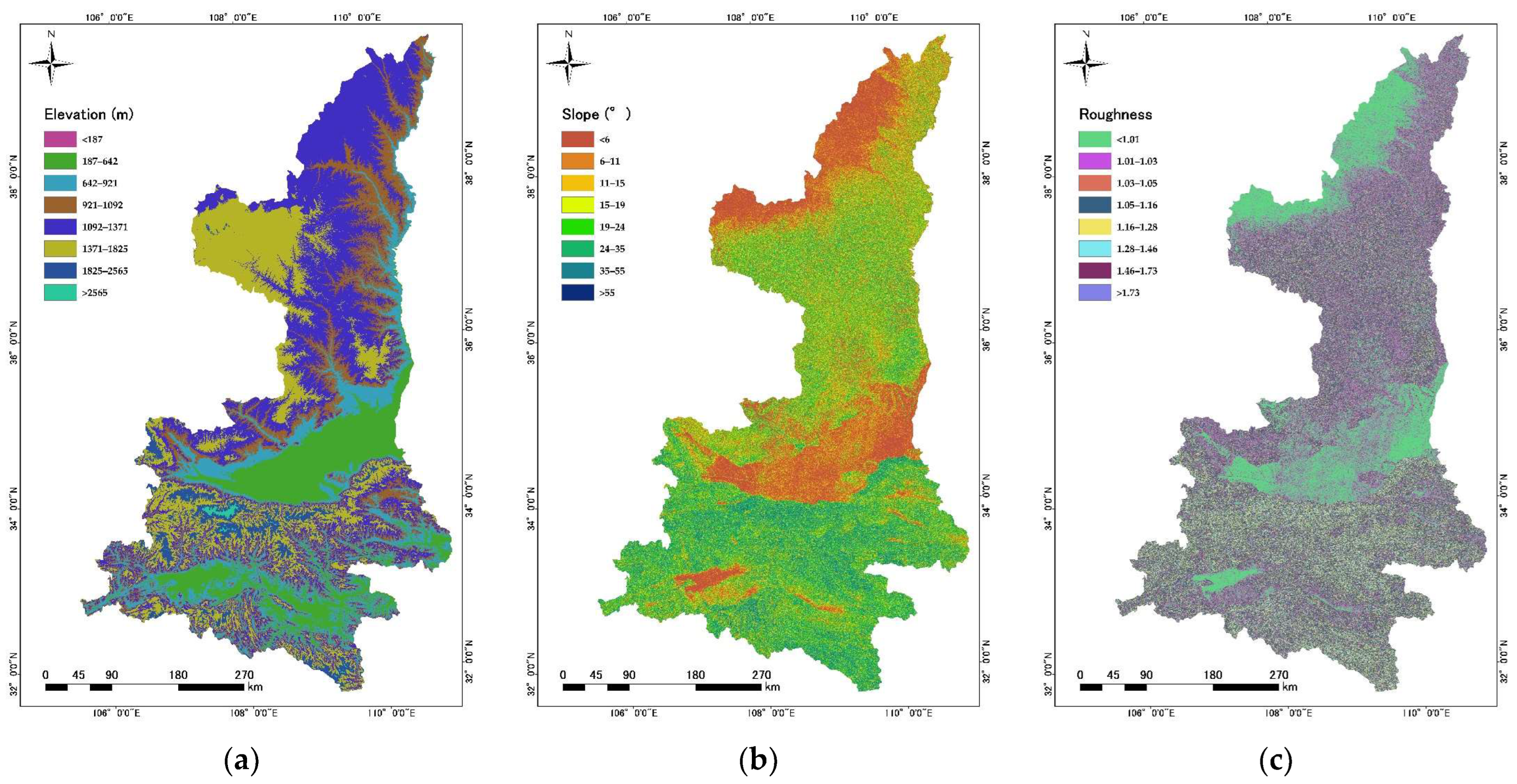
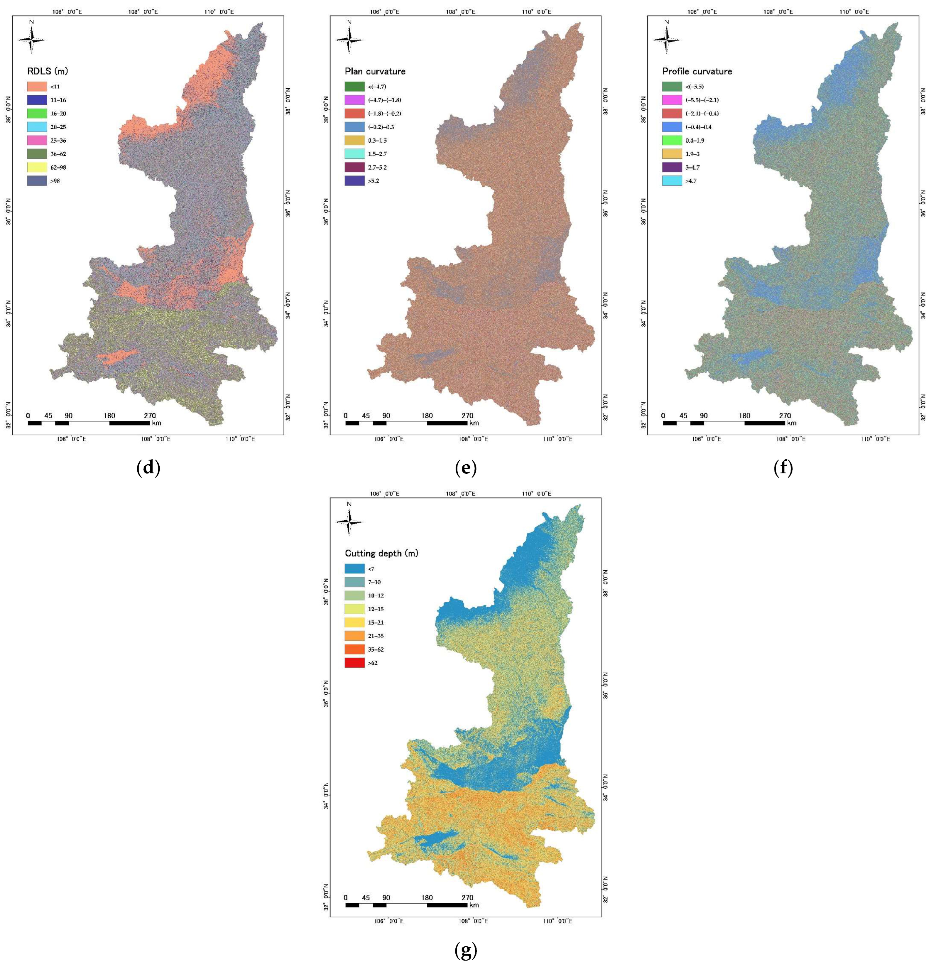
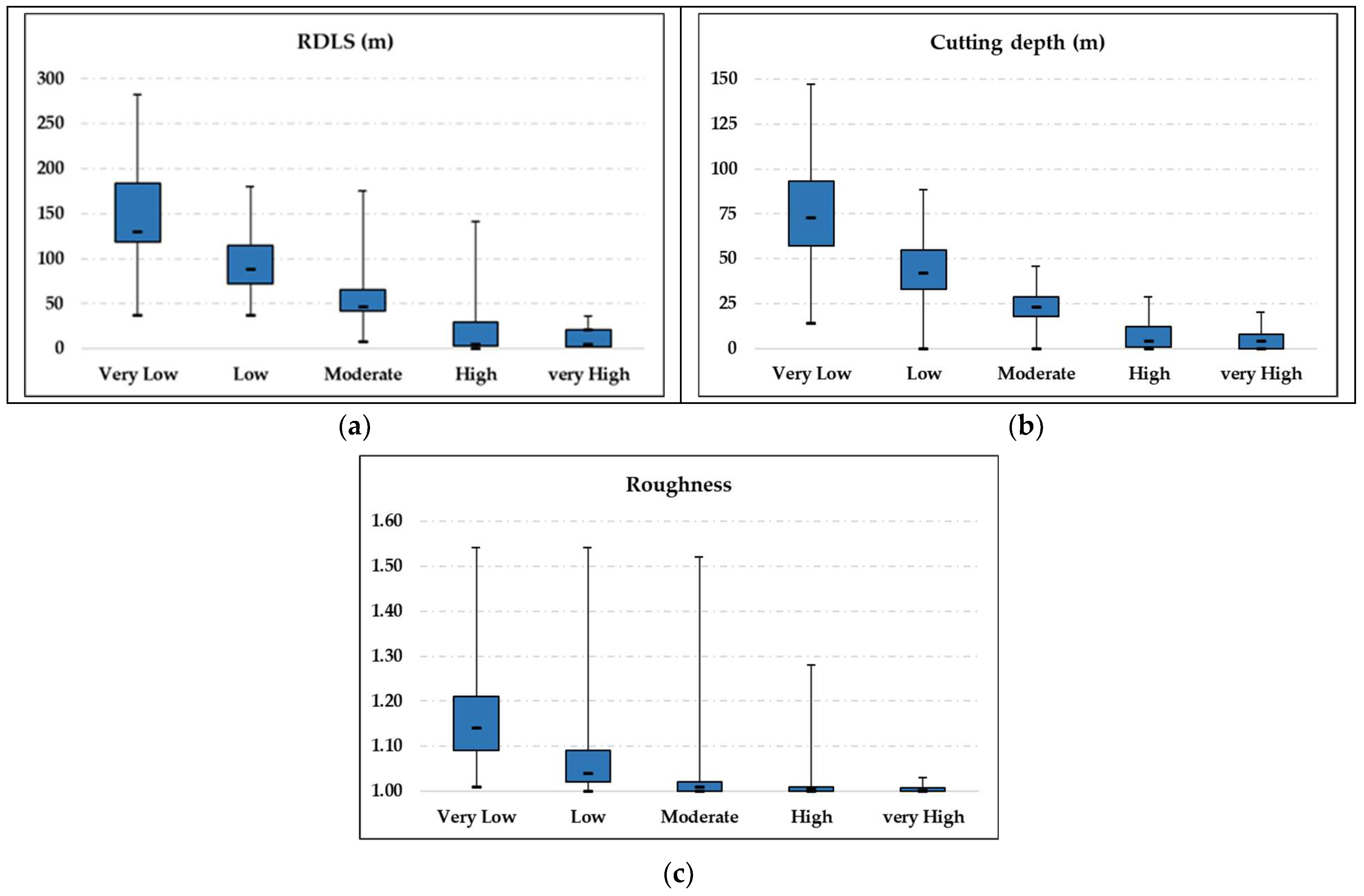
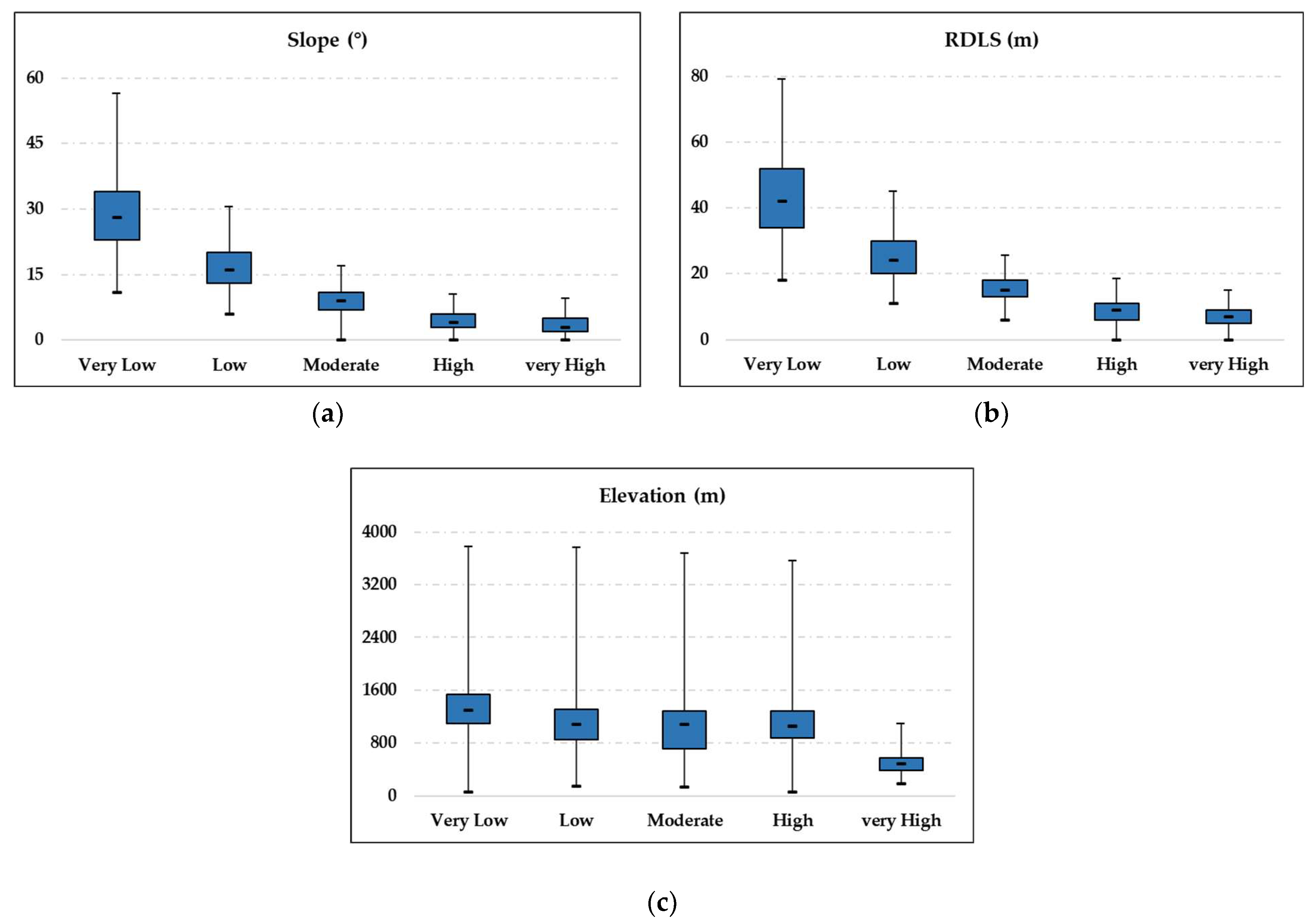
2.3. Geomorphological Predictive Factors

Archaeological site predictive factors, which may influence site occurrence or absence, need to be selected as explanatory or independent variables for APM [4,13,36]. In research about the relationship between archaeological/historical sites and their surrounding terrain, topography is often regarded as one of the most influential parameters [37]. In addition, the existing research results [12,13,14,15,16] have shown that topographic factors, as well as the distance from bodies of water, play an important role in the performance of the predictive model. To consider the influence of these factors, seven topographic factors and one hydrological factor were selected for this study, as explained below.
This study utilizes Digital Elevation Models (DEMs) to understand topographic conditions. DEMs for Japan are provided by the Geospatial Information Authority of Japan, with an original resolution of 10 m. To facilitate the comparison with China, we re-sampled the DEMs at a resolution of 30 m and rectified them to the northern Universal Transverse Mercator projection zone 54. For China, the 30 m-resolution ASTER GDEMs are used and projected as World Geodetic System 1984 Albers.
Generally, using the topographic data of an original point to represent that of a region offers a one-sided view. Considering that the archaeological sites in both study areas range in size from several meters to hundreds of meters, and the detailed outline of each archaeological site is unavailable, we used the ArcGIS 10.6 focal statistics tool to obtain the topographic factors for each site. The tool employs overlapping neighborhoods to calculate a statistic for the cells within a specified neighborhood around each input cell [38]. In our case, the topographic data for each archaeological site were calculated as the mean of factor values in a 3 × 3 neighborhood around the central point of each archaeological site in an input raster. In this way, the one-sidedness caused by calculating topographic data from a point can, to some extent, be avoided.
This study has selected seven topographic factors to explore the relationship between the locations of ancient sites and topography. These factors are elevation, slope, roughness, RDLS, plan curvature, profile curvature, and cutting depth (Figure 2 and Figure 3). Elevation and slope are fundamental properties applied in topography analysis, and the latter is calculated using the Slope Tool of ArcGIS software 10.6. Roughness reflects the degree of ground fragmentation in a macro-region, which is calculated as the ratio of the surface area of a cell to its projected area on the horizontal plane [39]. RDLS represents the difference between the highest and lowest values in the DEM around a central point within a specific neighborhood [40]. Plan curvature is determined as the contour curvature [40], perpendicular to the direction of the maximum slope. Profile curvature is slope profile curvature [40] parallel to the direction of the maximum slope. Both curvatures are computed using the Curvature Tool of ArcGIS 10.6. Cutting depth refers to the difference between average and minimum elevations in a given neighborhood, which reflects surface erosion [39]. In this study, the size of the neighborhood is set to 90 × 90 m, which is a moving window of 3 × 3 cells. Initially, several other topographic factors, such as the slope aspect and the variance coefficient in elevation, were also chosen and tested using statistical analysis; however, they were eliminated as they had almost no regularity with the distribution of archaeological sites.
Data on major rivers in Japan were collected from the online database of MLIT (Ministry of Land, Infrastructure, Transport, and Tourism) of Japan. The data for Shaanxi, China, were obtained from the Resource and Environmental Science Data Center of the Chinese Academy of Sciences. To clarify the use of the hydrological factor, the fact that the waterways have changed constantly throughout history means that the main rivers are considered stable and can be explored in this research (Figure 4). These rivers are typically larger than other rivers and play an essential role in terms of river area and runoff. Here, we use the distance between the archaeological sites and the major river to evaluate the water availability and input this into the predictive model as a hydrological factor.

3. Methodology

3.1. Selection of Predictive Factors

To assess whether selected factors have a significant association with archaeological sites, we employ Pearson correlation analysis. Only factors that exhibit significant correlations (p < 0.05) are retained. Checking for multicollinearity among predictive factors is an essential step in predictive modeling but is often overlooked [4]. Strong collinearity between predictors can lead to an overestimation of the predictive power of the model [4] or weaken model interpretability [41]. Therefore, we employed the variance inflation factor (VIF) and tolerance (TOL) to detect collinearity between predictors. VIF values greater than 10 or TOL values close to 0.1 indicate the presence of strong multicollinearity [42,43]. Based on the result, we retained only meaningful factors for modeling.

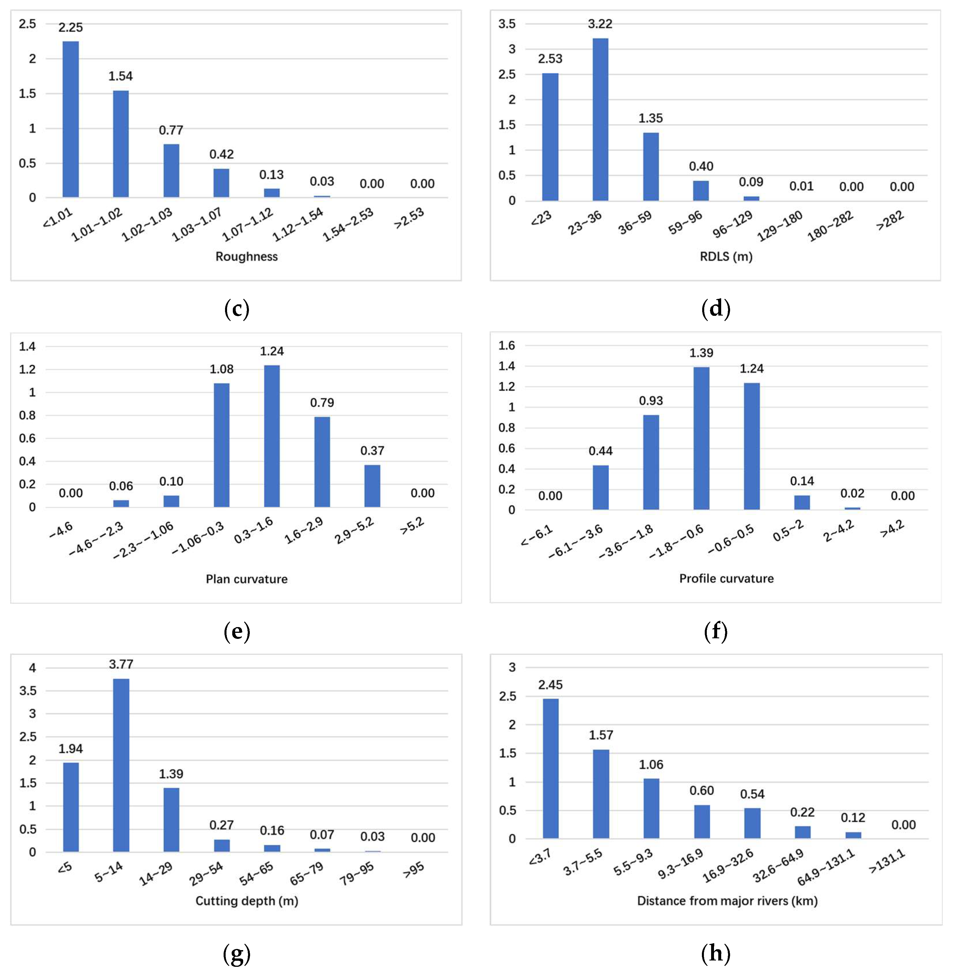
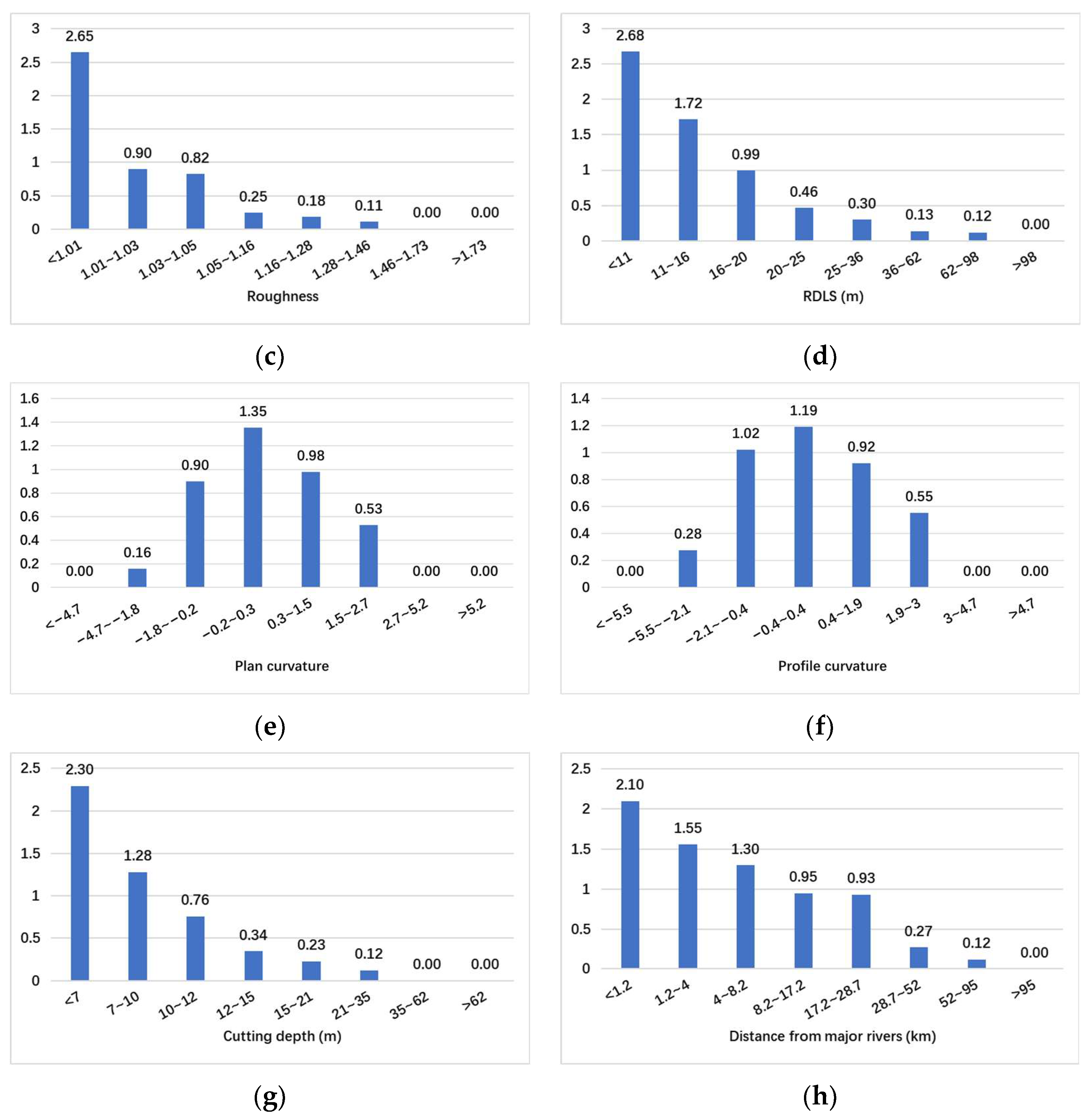
3.2. Frequency Ratio (FR)

The FR model is a bivariate statistical method that can indicate the susceptibility of related factors under certain conditions based on quantitative statistical results [44]. Due to its conceptual simplicity and straightforward calculation of the susceptibility index, FR is widely used in geoscience, such as landslide susceptibility mapping [45,46,47] and mapping ground subsidence potential [48]. In our study, we employ the geometrical interval classification method offered by ArcGIS 10.6 to classify predictors and optimize them accordingly. The FR formula is as follows:
F R i , j = N p i x ( S i , j ) / j N P i x ( S i , j ) N p i x ( N i , j ) / j N P i x ( N i , j )
where N p i x ( S i , j ) is the number of pixels containing archaeological sites within class j of factor i ; j N P i x ( S i , j ) is the number of total pixels containing archaeological sites in the study area; N p i x ( N i , j ) refers to the number of pixels of class j of factor i ; and j N P i x ( N i , j ) is the number of total pixels in the study area.
The FR value represents the degree of the influence of each input factor on the occurrence of archaeological sites: F R i , j > 1 indicates a strong correlation with site occurrence, while F R i , j < 1 indicates a low correlation.
The summation of each factor’s ratio is used to calculate the site probability (SP) using the following Equation:
S P = F R i
where F R i is the FR value of different classes within factor i , and the S P is an index of site probability.

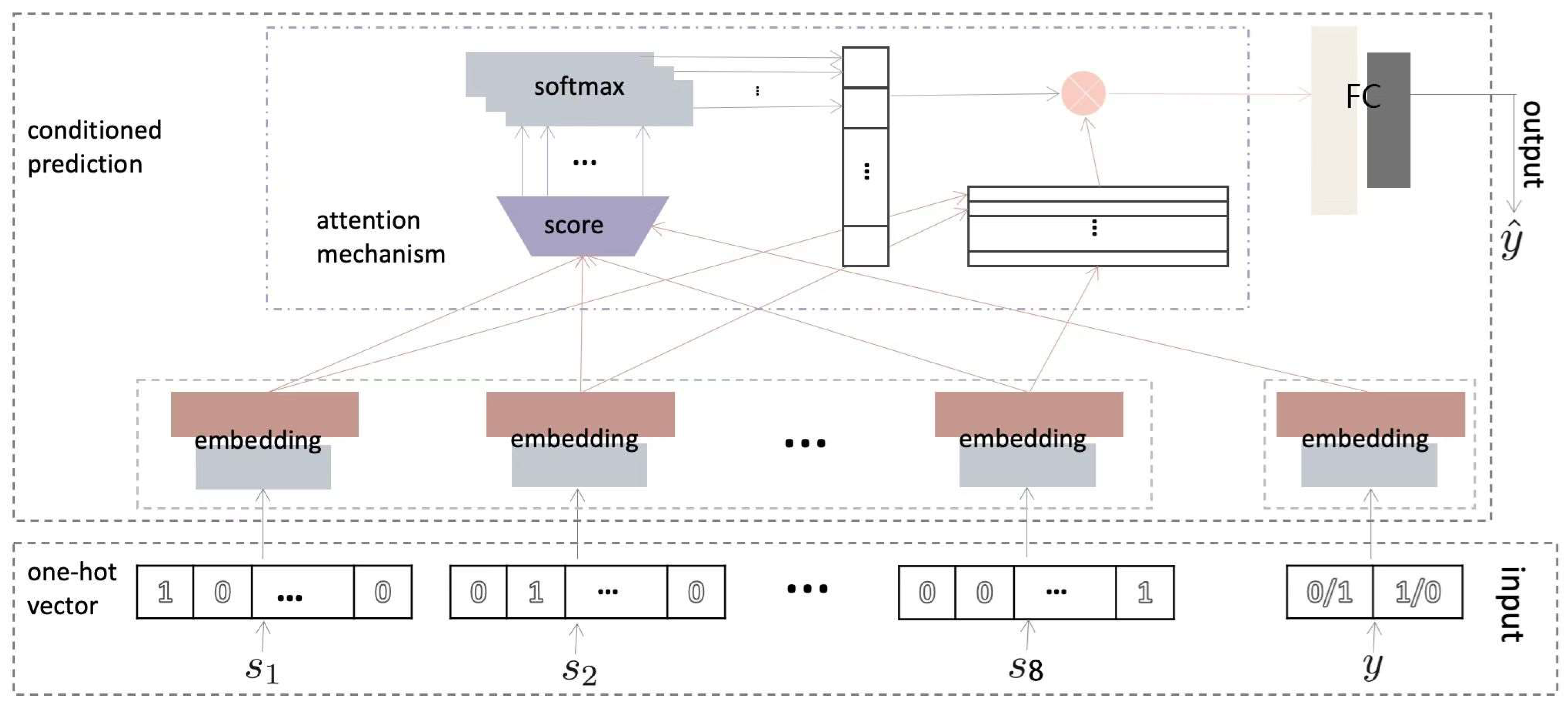
3.3. Hybrid Model of Attention Mechanism and Frequency Ratio (AM_FR)

Deep learning using artificial neural networks with representation learning is a subfield of machine learning. Deep learning methods perform automatic feature extraction from raw data and have had success in many areas, such as classification [49,50], prediction [51,52], and natural language processes (NLP) [53,54]. The attention mechanism was formally proposed in 2014 when Bahdanau et al. [55] first utilized it for machine translation in NLP [56]. Inspired by the human visual mechanism to focus on a specific area of an image in high resolution while perceiving surrounding areas in low resolution [56], the attention mechanism in the neural network pays more attention to relevant information while decreasing the concentration of irrelevant information. In this section, we propose a novel data-driven predictive model for archaeological site locations, as shown in Figure 5, which incorporates all input factors and jointly learns how these topographic and hydrological factors affect the locations of archaeological sites. The proposed model intuitively scores and selects the most relevant factors using an attention mechanism conditioned on class labels of archaeological sites.

3.3.1. Problem Formulation

We assume there are I sites in our dataset. For each site i { 1 , 2 , , I } , the observation data are input factors s i = { s i m | m = 1 , 2 , , M } and class labels y i . We aim to estimate the class labels of sites while learning the different weights of the input factors in relation to archaeological sites, considering the obtained topographic and hydrological factors. To this end, we obtain the posterior distribution p ( y ^ | s ) through our conditional attention-based neural methods:
p ( y ^ | s ) = i p ( y ^ i | s i ) = i p ( y ^ i | s i , w i ) p ( w i | s i , y i )
where w i indicates how the input factors interact with the locations of archaeological sites.

3.3.2. Model Architecture

We conduct the one-hot encoding [57], utilizing the one-hot vector v i m to indicate each inputting factor s i m . v i m is a vector of ones and zeros without an ordinal relationship, and its length is determined by the number of input factors. Likewise, we generate a one-hot vector u i with a length of two for labels. Then, we embed v i m and u i , respectively.
f i m = ϕ m ( ϕ ˜ m ( v i m s i m ; ω ˜ m ) ; ω m )
h i = ϕ 0 ( u i ; ω 0 )
Here, f i m is the feature of inputting factor s i m , h i is the feature of the class label, ϕ ˜ m , ϕ m , and ϕ 0 are the fully connected layers; the latter two have a dropout value of 0.50 and ReLU non-linearity. ω ˜ m , ω m and ω 0 are their respective weights.
To determine the interactions between the archaeological sites and the input factors, we introduce an attention mechanism [59] conditioned on the class labels of archaeological sites to learn the different weights of the input factors. The attention feature a i m is derived from f i m and h i .
a i m = e x p ( S ( f i m , h i ) ) m e x p ( S ( f i m , h i ) )
Here, a i m is a tensor [60] with size M which indicates the weights of the input factors. S ( ) is the matrix product as follows:
S ( f i m , h i ) = ( f i m ) T h i
Then, H i , a feature representing all input factors, is derived by multiplying a i m with f i m .
H i = m a i m f i m
H i is the weighted average tensor over all the features f i m . H i is utilized to identify the probability of archaeological site occurrence as follows:
y ˜ i = Φ 1 ( H i ; ω Φ 1 )
y ^ i = ε ( Φ 2 ( y ˜ i ; ω Φ 2 ) )
where Φ 1 ( ) and Φ 2 ( ) are the fully connected layers with ReLU non-linearity, where the former also has a dropout value of 0.50; their weights are ω Φ 1 and ω Φ 2 , respectively. ε ( ) is a softmax function and y ˜ i is the probability distribution over the predicted class of the archaeological site. y ^ i consists of two classes and sums to 1. The larger probability indicates whether the current location is an archaeological site.

3.3.3. Implementation

We utilize Binary Cross-Entropy [61], a distinction measurement between two possible distributions (ground truth and predicted distributions) used when the number of classes is two, as a loss function of our model. Our model is implemented using PyTorch under Ubuntu 16.04LTS with a GTX 1080GPU. The embedding size of ϕ ˜ m ( ) and Φ 1 ( ) is set to 32, while that of the other fully connected layers is set to 64. The proposed method is trained for 1000 epochs with a batch size of eight. We train the model end-to-end with an AdaGrad optimizer at a learning rate of 0.01. We also clip the gradients of the model with a maximum threshold of five to stabilize the training process. Finally, the weight of each predictive input factor was obtained; this was then applied to the APM model as the index of weight.
As noted, we propose a weighted archaeological predictive model by integrating the conditional attention mechanism with the FR model and consider the weight of each classification within each factor, as well as the weight of all of these factors. This weighted calculation can be implemented in ArcGIS 10.6 using the tool for geographically weighted overlay analysis. The site probability is calculated by Equation (11):
S P = W F R i
where W is the weight of each factor generated from the proposed conditional attention mechanism neural network, F R i is the frequency ratio of different classes within factor i , and S P is an index indicating the probability of site occurrence.

3.4. MaxEnt

MaxEnt is a machine learning model that combines information theory and statistics to select the best model from all possible models [62,63]. MaxEnt identifies the model with the maximum entropy in the condition set that satisfies the site presence constraints (e.g., geomorphological factors in this study) [64]. The model can work with only known site data, making it ideal for cases with a presence-only feature. This study used MaxEnt software version 3.3.3k to model the probability of archaeological site presence based on geomorphological and hydrological factors. The mathematical steps of the modeling are as follows.
Assume C as the set of models satisfying all constraints f i :
C = { P | E P ( f i ) = E P ˜ ( f i ) , i = 1 , , n }
where P refers to experience distribution, and f i is the feature function corresponding to the input factor n (= 8 in this study) on the presence of archaeological sites, defined as:
f i = { 1 , 0 ,
The model is constrained by the eight factors with setting the expectation from the observed data ( E P ( f i ) ) to be equal to the model’s expectation ( E P ˜ ( f i ) ) under the maximum entropy condition. Entropy, according to Phillips and Borda [63,65], is:
H ( P ) = x X P ˜ ( x ) ln P ˜ ( x )
where x is a random location within the study area X , and P ˜ is the expected probability distribution. The logarithm function here makes independent sources to be additive (e.g., x within X ). This equation sets the sum of probabilities to be one. The probability distribution of archaeological site presence P is as follows:
P = arg max P C H ( P )

3.5. Model Evaluation

The predictive performance of the two models for the two study areas is compared using the area under the receiver operating characteristic curve (AUC), a commonly used statistical parameter [66]. It measures the overall performance of a model across all possible classification thresholds. A higher AUC value close to 1 indicates that the model has a high true positive rate and a low false positive rate and can accurately distinguish between positive and negative cases [67]. AUC is calculated for the training and test data, respectively.
To evaluate model performance, we also use Kvamme’s Gain, which gives a ratio of the precision of a model against its accuracy [68] as:
Kvamme’s Gain = 1 − (% of the area with high probability/% of sites with high probability).
This metric evaluates whether the probability area is small enough compared to its accuracy. A smaller probability area with more archaeological sites will generate a greater gain value close to 1, which suggests that the model has a good predictive ability. A zero-gain value indicates that the model’s predictions are no better than guesses.

4. Results

4.1. Selected Predictive Factors
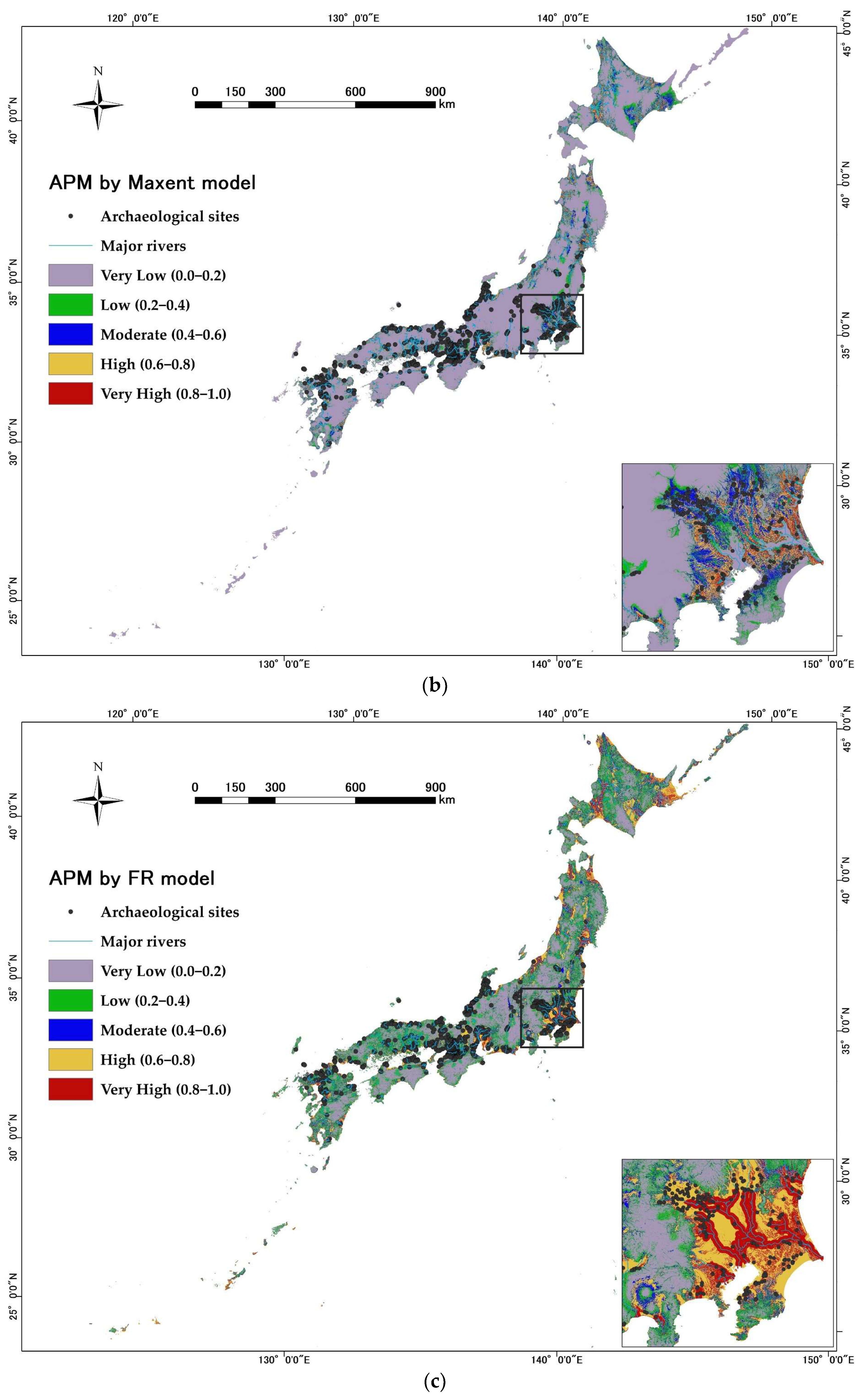
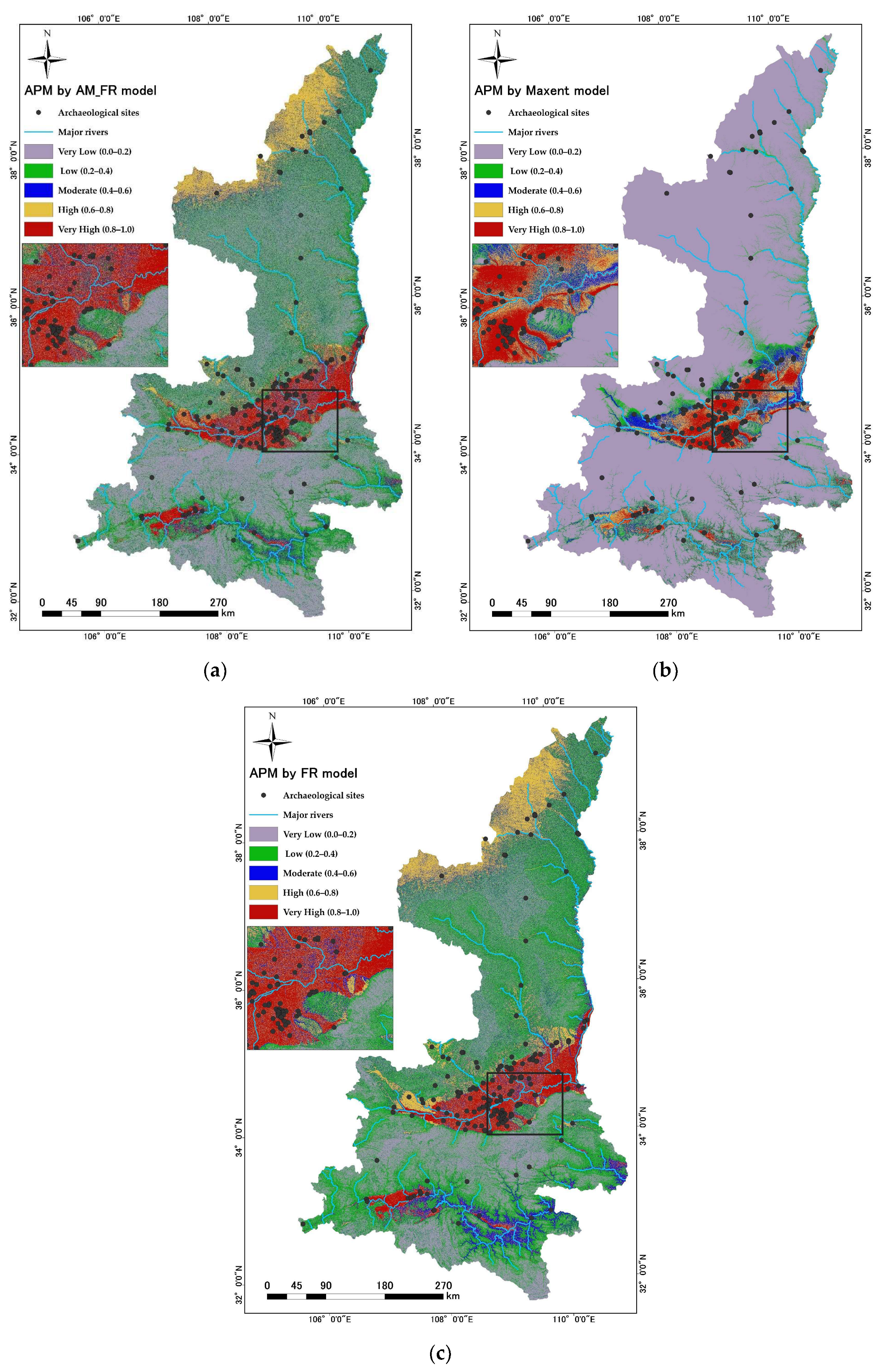
Table 1 presents the results of Pearson correlation analysis of the predictors. The aspect factor is not strongly correlated with archaeological sites in both the Japanese and Shaanxi study areas, with p > 0.05, while all the other factors exhibit strong correlations. Consequently, the predictors used in the subsequent steps are those other than the aspect.
Table 2 shows that the VIF and TOL values for all the factors except for elevation variation were within the acceptable range (VIF < 10 or TOL > 0.1), indicating no significant multicollinearity among them. Consequently, the eight factors other than elevation variation and aspect were retained.

4.2. APM by FR

Based on the classification of each independent input factor, FR indexes are calculated (Figure 6 and Figure 7). The FR values quantify the degree of correlation, and the input factor classes with an FR value of >1 show a markedly high correlation with the archaeological site.
It was found that the elevation class <133 m shows a higher correlation with archaeological sites in the study area of Japan, while in Shaanxi, China, the same is true of the range 187–921 m. As for slope and roughness, the FR values are more or less the same in Shaanxi, China, and Japan, which indicates that archaeological sites in these two study areas tend to be located in plains-type regions with gentle slopes; these slopes are commonly less than 15°. For the RDLS in Japan, the class of 23–36 m has the most significant impact on archaeological sites, followed by the class <23 m and 36–59 m. Meanwhile, in Shaanxi, China, the class <11 m has the greatest impact on archaeological sites, followed by the classes 11–16 m and 16–20 m. The plan curvature values from −1.06 to 1.6 show a stronger correlation with archaeological sites in Japan; the corresponding class in Shaanxi, China, is −0.2 to 3. In Japan, the profile curvature with values −1.8 to 0.5 is highly correlated with archaeological site occurrence, while in Shaanxi, China, the same is valid for values −2.1 to 0.4. In terms of cutting depth, in the study area of Japan, the classes of <5 m, 5–14 m, and 14–29 m had FR values greater than one, showing a significant contribution to the archaeological site’s occurrence; meanwhile, in Shaanxi, China, such classes are <7 m and 7–10 m. This indicates that the archaeological sites of both study areas are commonly located in areas with low erosion and a gentle cutting of the ground surface; the level of gentleness tends to be lower in Shaanxi, China, than in Japan. The distance from major rivers is also a major input factor influencing the distribution of archaeological sites in both study areas. The FR values of the first three classes in each study area are all greater than one, indicating a strong correlation with the locations of archaeological sites. Moreover, in both study areas, the distance from major rivers is negatively correlated with the distribution of archaeological sites. This indicates that archaeological sites are densely located close to major rivers in Japan as well as in Shaanxi, China, since people considered water availability or the strategic role of rivers when establishing a site.

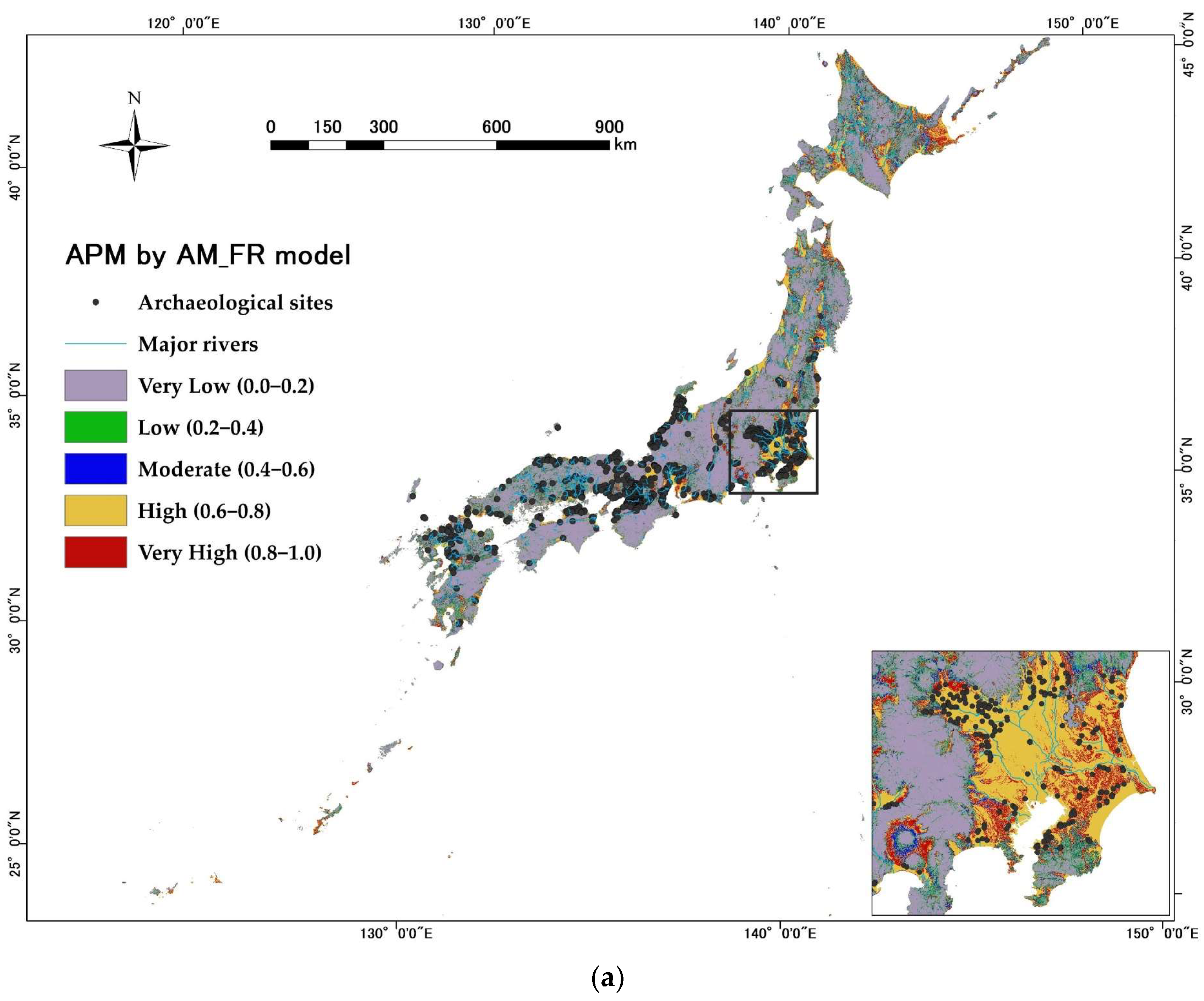
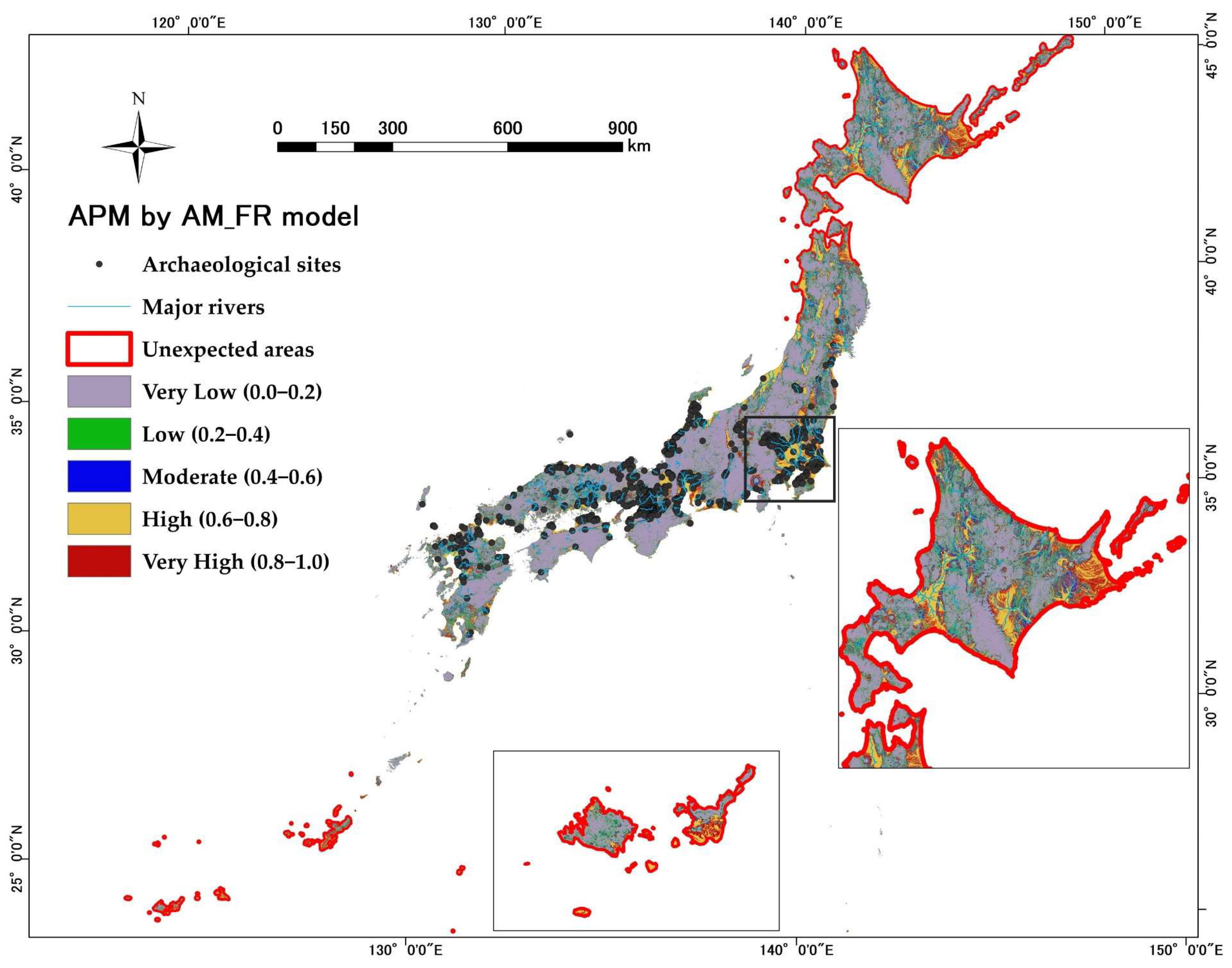
4.3. APM by the AM_FR Model

Concerning the sensitivities of factors in determining the likelihood of an archaeological site’s occurrence, a conditioned attention mechanism was utilized for weight determination. Table 3 shows the weighting results, indicating that the sensitivities of archaeological sites to the input factors are different under the distinct topographic conditions in the two study areas. In Japan, the relationship between the site locations and the input factors can be quantified by values from 0.0145 to 0.3356, while in Shaanxi, China, the values range from 0.0809 to 0.2878. A higher value implies a higher correlation. In Japan, the factors with the most significant correlations with archaeological sites are RDLS and cutting depth, followed by roughness; in Shaanxi, they are slope and RDLS, followed by elevation (Table 3). SP for Japan is expressed as Equation (17), and that for Shaanxi is defined as Equation (18):
APM = 0.0145ElevationFR + 0.0714 SlopeFR + 0.0997RoughnessFR +
0.3356RDLSFR + 0.0424Plan_CurvatureFR + 0.0717Profile_CurvatureFR +
0.2813Cutting_depthFR + 0.0834Distance from major riversFR
APM = 0.1223ElevationFR + 0.2878 SlopeFR + 0.0948RoughnessFR +
0.1524RDLSFR + 0.0809Plan_CurvatureFR + 0.0916Profile_CurvatureFR +
0.0869Cutting_depthFR + 0.0833 Distance from major riversFR

4.4. APM by MaxEnt

The use of MaxEnt software enables the creation of a predictive map and the evaluation of factor contribution to modeling. Table 4 displays the factor contributions to the modeling using the training dataset. In the Japanese modeling, major contributors are roughness (33.7%), RDLS (24.3%), and cutting depth (16.5%), while in the Chinese modeling, they are elevation (25.7%), slope (23.8%), and RDLS (18.5%).

4.5. Model Evaluation

The AUC values for the test data indicate that the AM_FR model has the highest accuracy in both study areas (see mean AUC values in Table 5). However, the AUC for the training data indicates the best performance of MaxEnt for China
Table 6 shows that all three models effectively identified regions with very high probability in both study areas. However, MaxEnt had a higher efficiency in identifying such regions, with a Kvamme’s Gain value of 0.92 for Japan and 0.89 for China. In comparison, the AM_FR and FR models had lower efficiency, with values of 0.78 and 0.72, respectively, for Japan and 0.84 and 0.83 for China.

4.6. Archaeological Predictive Maps and Statistics

The predictive maps for each study area based on the two models are generated with the help of ArcGIS 10.6 software (Figure 8 and Figure 9). In order to ensure the fairness of the comparison, the output susceptibility maps are divided into five categories using the equal interval classification method, classifying probabilities ranging from 0 to 1 into five classes.
Figure 8 shows that the high and very high probability classes are mainly concentrated in two parts of Japan. One is in the Kanto region, which includes Tokyo, Chiba, and Saitama Prefectures; the other is in the Kansai region, which includes Kyoto, Osaka, and Nara Prefectures. To this day, these areas are active political, economic, and cultural centers. Very low and low probability classes mainly covered the entire study area. Moderate probability classes are generally distributed in the areas where those low and very low-class areas intersect with the high and very high-class areas. The statistics of area percentage for each probability class are shown in Table 6. For the AM_FR model, the very low probability class accounts for the largest area (42.67%), followed by high (18.09%), low (19.12%), moderate (11.20%), and very high (8.92%). For the FR model, the very low probability class accounts for the largest area (31.62%), followed by low (24.04%), high (19.37%), very high (14.20%), and moderate (10.77%). For the Maxent model, the area percentage consistently decreases from very low to very high classes: 70.07%, 11.89%, 14.19%, 6.46%, and 2.81%, respectively.
The very high and high probability classes in Shaanxi, China (Figure 9) are mainly concentrated in three regions: namely, the northwestern, central, and southwestern parts of the study area, especially in the central part, where the ancient city of Xi’an is located. Moderate probability classes are evenly distributed throughout the study area. Very low and low probability classes are, respectively, concentrated in the northern and southern parts of the study area. According to Table 6, for the AM_FR model, the very low probability class accounts for the largest area (35.14%), followed by low (28.11%), high (15.91%), moderate (13.16%), and very high (7.68%). For the MaxEnt model, the very low probability class accounts for the largest area (72.10%), followed by low (15.66%), very high (5.32%), high (4.87%), and moderate (2.05%). For the FR model, the low probability class accounts for the largest area (36.35%), followed by very low (23.79%), high (17.06%), moderate (15.54%), and very high (7.25%).
To understand the relationship between archaeological site locations and the highly correlated topographic factors, zonal statistical analyses are conducted for those topographic raster data to calculate the statistic value based on the classification area of the predicted map. The results show a linear correlation between topographic factors and archaeological site presence, and their characteristics are more or less the same, as the higher the average value of each topographic factor, the lower the probability of site presence (Figure 10 and Figure 11).

5. Discussion

The current study validated the applicability of the proposed AM_FR model through its application to Japan and Shaanxi, China, with different terrain conditions. For both areas, the AM_FR performed slightly better than the MaxEnt and FR based on the values of AUC (Table 5). The deep learning AM_FR method better captures the highly correlated environmental factors in the prediction model, locking the target and narrowing down the areas with a high probability of archaeological site occurrence. At the same time, the FR model has also provided a reasonably good result, indicating that the correlations between the environmental factors and archaeological site occurrence are strong and detectable even from a traditional statistical method. However, in terms of model efficiency, Kvamme’s Gain was used as a measure of model efficiency in APM, and MaxEnt was found to be more effective than AM_FR and FR in identifying regions with a very high probability of archaeological site occurrence in both study areas. Nevertheless, this comes at the cost of many sites being classified as moderate and low probability areas, meaning that some true archaeological sites may be missed in practice.
According to the importance of each predictive factor determined by the APM processes, topographic deviations from the horizontal flat surfaces play an essential role in deciding archaeological site locations. The three most important factors for Japan (RDLS, cutting depth, and roughness) and the two of the three most important factors for Shaanxi (RDLS and slope) (Table 3 and Table 4) represent deviations from horizontal flat surfaces in a broad sense. Their blatantly negative relationships with the existence likelihood of archaeological sites (Figure 10 and Figure 11a,b) show that these sites tend to be located in open, gentle, and flat terrain, such as lowland areas or basins away from hills and mountains. This may reflect the needs of ancient people for a better living environment in relation to resource-sharing strategies, transportation, water availability, and agricultural activities. As known, widely gentle areas without distinctive inclines, declines, or severe downcutting are beneficial for human activity. They were crucial in the absence of advanced means of transportation at that time. They also benefit agricultural activities because of high water availability and the deposition of fine sediments containing micronutrients.
However, among the factors representing deviations from the horizontal and flat surface, only RDLS strongly influences both Japan and Shaanxi. In Japan, the cutting depth and roughness are more influential, whereas sloping is dominant in Shaanxi. The cutting depth and roughness strongly reflect local topographic undulations with short wavelengths rather than overall inclination. It is understandable that if local topographic undulations are high, the earthen keyhole-shaped tombs typical in Japan are difficult to construct. Their construction by embankment needs a relatively wide, continuously flat surface. In contrast, archaeological sites in Shaanxi are mainly composed of bricks and rocks and have various structures and shapes that could be adjusted to land surfaces with local slight topographic undulations. Besides, the overall slope becomes more critical in Shaanxi. Based on Figure 11a, a slope value of around 5° is most favorable for the archaeological site occurrence, and a slope greater than 27° is highly unfavorable. A Chinese study assessing land suitability [69] noted that areas steeper than 25° are unsuitable for farming, whereas areas gentler than 5° are suitable for cultivation and human habitation, suggesting that the archaeological sites tended to be constructed in areas with strong human activities. The archaeological sites in Shaanxi differ from the Japanese sites in that they include temples and palaces, as well as tombs. Temples and palaces usually occur in populated areas because they have more frequent visitors than tombs. This may explain why the sites in Shaanxi are more concentrated in lower-slope areas with enhanced human activities.
In Shaanxi, elevation also plays a significant role in determining the distribution of archaeological sites. As shown in Figure 11c, lower elevations correspond to more sites, particularly abundant in the lowest elevation zone. Elevation as a geographical parameter differs from the four parameters mentioned above because it is independent of flatness by definition. Shaanxi is located in a continental inland area, with significant variations in daily and yearly temperatures and more limited rainfall compared to Japan, with a maritime, more moderate climate. Therefore, higher areas in Shaanxi with occasional lower temperatures and water availability are particularly unfavorable for human activities.
The negative correlations shown in Figure 10 and Figure 11 are consistent, except for partial positive correlations for the high and very high probability classes of RDLS and cutting depth in the AM_FR statistics for Japan (Figure 10a,b). One possible explanation for this exception is the construction of the archaeological sites. Because the Japanese sites are earthen tombs, their elevations are included in the analyzed DEMs. Therefore, the dense distribution of the sites leads to higher topographic undulations. Overall, this study has examined the effects of natural topographic conditions that already existed before site construction, as evidenced by the negative correlations in Figure 10 and Figure 11. However, the artificial topographic change due to the construction of earthen mounds in Japan may also affect the results slightly. Another possible explanation is the preference of ancient people for slightly complex terrains. For example, in Belgium, the Early and Middle Bronze Age populations built their burial monuments on more prominent lands rather than in very flat positions [37]. As noted, however, the comparison between Japan and Shaanxi indicates that continuously horizontal and flat surfaces were more favored in Japan, suggesting that the first explanation is more acceptable.
This paper focuses on the effects of topographic factors on human activities, which in turn affect the distribution of archaeological sites. However, social and cultural elements could also directly affect the site distributions, which looks evident in the Japanese case. Although some 5000 keyhole-shaped tombs are distributed in most of the Japanese archipelago [23,70], such tombs scarcely exist in 4 out of 47 prefectures in Japan: Hokkaido, Aomori, and Akita in the north, and Okinawa in the south (Figure 12), because of historical backgrounds related to cultural stages and political regimes. The main island of Hokkaido is away from the other territories of Japan. During the Kofun period, when keyhole-shaped tombs were constructed in most other regions in Japan, Hokkaido was under a more primitive culture analogous to what the other regions experienced before the Kofun period (Jōmon culture) [71,72]. Therefore, people in Hokkaido did not have a custom or tradition for constructing keyhole-shaped tombs at that time. The lack of keyhole-shaped tombs in Aomori and Akita can be attributed to politics. These areas were controlled by the Emishi people during the Kofun period, who were hostile to the Yamato kingdom, ruling most other regions in Japan [73,74]. The situation in Okinawa was similar to the northern prefectures in that the culture of the Kofun period hardly extended to the southern Ryukyu Islands, and a unique political and cultural system existed in the islands [75]. The predictive maps of keyhole-shaped tombs for the whole of Japan generated by the AM_FR, Maxent, and FR models show some high and very high probability areas in these four prefectures (Figure 8 and Figure 9) because only natural factors were considered in the models. This example indicates that the results of archaeological predictive modeling should be evaluated carefully when marginal areas surrounding the core area are included in the constructed predictive maps.

6. Conclusions

This study has proposed a weighted archaeological predictive model. The model utilizes the weights of input factors obtained from the conditional-attention-based method and the weight of each class within inputting factors obtained from the FR model. The performance of the new model in Japan and Shaanxi, China, was evaluated using AUC values and Kvamme’s Gain and compared with that of a separate FR model and MaxEnt. In general, the AM_FR model showed more satisfactory performances in both study areas. Therefore, the development of the new model was meaningful. The widely used MaxEnt and the more traditional FR model still provided reasonably good results. Therefore, multiple modeling methods indicate that archaeological sites in the two study areas tend to occur in areas with certain environmental characteristics, supporting the notion that archaeological sites are not randomly distributed [4]. Admittedly, our models have proven successful in identifying the sites under the current study, but their effectiveness in identifying other site types, such as villages or hunting camps, is yet to be fully determined. Since tombs and places of worship do not require proximity to food or water sources for their specific uses, they have a specific history of landscape use, diverging from those typically linked to settlements or hunting grounds.
Exploring the relationship between the locations of archaeological sites and the eight geomorphological and hydrological factors has revealed that archaeological sites in the two study areas are highly correlated to some topographic factors, suggesting that the distribution of the archaeological sites reflects local conditions. In Japan, the three main factors highly correlated to the location of archaeological sites are RDLS, cutting depth, and roughness, while in the Chinese study area, they are slope, RDLS, and elevation. All these factors are negatively correlated with the probability of archaeological site occurrence, meaning that horizontal and flat land surfaces favored human activities, including transportation, agriculture, and water usage, and in turn, the construction of archaeological sites. The dominance of somewhat different factors in the two countries may reflect the structure of the archaeological sites and regional climates.

Author Contributions

Conceptualization, Yuan Wang and Takashi Oguchi; methodology, Yuan Wang and Xiaodan Shi; formal analysis, Yuan Wang and Takashi Oguchi; writing—review and editing, Yuan Wang., Takashi Oguchi and Xiaodan Shi. All authors have read and agreed to the published version of the manuscript.

Funding

This work was supported by JSPS Grants-in-Aid for Scientific Research (18K18536).

Informed Consent Statement

Not applicable.

Data Availability Statement

The 10m-resolution DEMs of Japan are openly available from the Geospatial Information Authority of Japan: “https://fgd.gsi.go.jp/download/menu.php (accessed on 28 November 2020)”. The 30m-resolution DEMs of Shaanxi, China are openly available from: “https://gdemdl.aster.jspacesystems.or.jp/ (accessed on 24 November 2020)”. Archaeological data are not publicly available due to privacy and ethical reasons.

Conflicts of Interest

The authors declare no conflict of interest.

References

  1. Kohler, T.A.; Parker, S.C. Predictive Models for Archaeological Resource Location. Adv. Archaeol. Method Theory 1986, 9, 397–452. [Google Scholar] [CrossRef]
  2. Vaughn, S.; Crawford, T. A predictive model of archaeological potential: An example from northwestern Belize. Appl. Geogr. 2009, 29, 542–555. [Google Scholar] [CrossRef]
  3. Nicu, I.C.; Mihu-Pintilie, A.; Williamson, J. GIS-Based and Statistical Approaches in Archaeological Predictive Modelling (NE Romania). Sustainability 2019, 11, 5969. [Google Scholar] [CrossRef] [Green Version]
  4. Yaworsky, P.M.; Vernon, K.B.; Spangler, J.D.; Brewer, S.C.; Codding, B.F. Advancing predictive modeling in archaeology: An evaluation of regression and machine learning methods on the Grand Staircase-Escalante National Monument. PLoS ONE 2020, 15, e0239424. [Google Scholar] [CrossRef] [PubMed]
  5. Wachtel, I.; Zidon, R.; Garti, S.; Shelach-Lavi, G. Predictive modeling for archaeological site locations: Comparing logistic regression and maximal entropy in north Israel and north-east China. J. Archaeol. Sci. 2018, 92, 28–36. [Google Scholar] [CrossRef]
  6. Willey, G. Prehistoric Settlement Patterns in the Viru Valley. Bur. Am. Ethnol. Bull. 1953, 155, 1–453. [Google Scholar]
  7. Hodder, I. Spatial Analysis in Archaeology; Cambridge University Press: Cambridge, NY, USA, 1976. [Google Scholar]
  8. Klesert, A. Intrasite Spatial Analysis in Archaeology. Am. Antiq. 1987, 52, 201–202. [Google Scholar] [CrossRef]
  9. Oguchi, T.; Saito, K. Relationship between distribution of landscape and natural/cultural environment in Poland based on GIS. Geogr. Res. Rep. Saitama Univ. 1999, 19, 41–59. [Google Scholar]
  10. Asada, H.; Matsumoto, J.; Lin, Z.; Oguchi, T. Relationship between Distribution of Residential Areas and Topographic Factors in the Sagarmatha Zone, Eastern Nepal. J. Geogr.-Chigaku Zasshi 2008, 117, 561–567. [Google Scholar] [CrossRef] [Green Version]
  11. Kondo, Y. An ecological niche modelling of Upper Palaeolithic stone tool groups in the Kanto-Koshinetsu region, eastern Japan. Quat. Res. Daiyonki-Kenkyu 2015, 54, 207–218. [Google Scholar] [CrossRef] [Green Version]
  12. Warren, R.E. Predictive Modelling in Archaeology: A Primer. In Interpreting Space: GIS and Archaeology; Allen, K.M.S., Green, S.W., Zubrow, E.B.W., Eds.; Taylor & Francis: London, UK, 1990; pp. 90–111. [Google Scholar]
  13. Kvamme, K.L. A Predictive Site Location Model on the High Plains: An Example with an Independent Test. Plains Anthr. 1992, 37, 19–40. [Google Scholar] [CrossRef]
  14. Stancic, Z.; Kvamme, K. Settlement pattern modelling through Boolean Overlays of social and environmental variables. In New Techniques for Old Times, Proceedings of the CAA Conference, 26th Annual Meeting, Barcelona, Spain, March 1998; (BAR International Series 757); British Archaeological Reports: Oxford, UK; pp. 231–237.
  15. Bauer, A.; Nicoll, K.; Park, L.; Matney, T. Archaeological site distribution by geomorphic setting in the southern lower Cuyahoga River Valley, northeastern Ohio: Initial observations from a GIS database. Geoarchaeology 2004, 19, 711–729. [Google Scholar] [CrossRef]
  16. Kondo, Y.; Sano, K.; Omori, T.; Abe-Ouchi, A.; Chan, W.L.; Kadowaki, S.; Naganuma, M.; O’ishi, R.; Oguchi, T.; Nishiaki, Y.; et al. Ecological Niche and Least-Cost Path Analyses to Estimate Optimal Migration Routes of Initial Upper Palaeolithic Populations to Eurasia. In The Middle and Upper Paleolithic Archeology of the Levant and Beyond; Nishiaki, Y., Akazawa, T., Eds.; Replacement of Neanderthals by Modern Humans Series; Springer: Singapore, 2018. [Google Scholar] [CrossRef]
  17. Verhagen, P.; Whitley, T.G. Integrating Archaeological Theory and Predictive Modeling: A Live Report from the Scene. J. Archaeol. Method Theory 2011, 19, 49–100. [Google Scholar] [CrossRef] [Green Version]
  18. Verhagen, P. Case Studies in Archaeological Predictive Modelling. Ph.D. Thesis, Leiden University Press, Archaeological Studies Leiden University, Leiden, The Netherlands, 2007. [Google Scholar]
  19. Ikeya, H. Debris flow and its countermeasures in Japan. Bull. Int. Assoc. Eng. Geol.-Bull. De L’Association Int. De Géologie De L’Ingénieur 1989, 40, 15–33. [Google Scholar] [CrossRef]
  20. Takagi, H. The Restoration of the Ancient Capitals of Nara and Kyoto and International Cultural Legitimacy in Meiji Japan. In The Meiji Restoration: Japan as a Global Nation; Cambridge University Press: Cambridge, NY, USA, 2020; pp. 249–265. [Google Scholar] [CrossRef]
  21. Kondo, Y. The Period of the Keyhole Tombs; Iwanami Publishing: Tokyo, Japan, 1983. [Google Scholar]
  22. Okada, H. Zempō-kōen fun. In Japanese Ancient History Dictionary; Daiwa Shobo Publishing: Tokyo, Japan, 2006. [Google Scholar]
  23. Yanagisawa, K. Zempō-kōen fun. In East Asian Archaeological Dictionary; Tokyodo Publishing: Tokyo, Japan, 2007. [Google Scholar]
  24. Ozawa, K. Classification of the Keyhole Shaped Tombs by Template Matching Method. IEEE Trans. Comput. 1978, 27, 462–467. [Google Scholar] [CrossRef]
  25. Hiroshi, T. Chiefly lineages in Kofun-period Japan: Political relations between centre and region. J. Antiq. 1990, 64, 923–931. [Google Scholar]
  26. Shiraishi, T. Study of the Kofun Tomb and Kofun Tomb Group; Hanawa Shobo Publishing: Tokyo, Japan, 2000. [Google Scholar]
  27. Wada, A. History of Japan 2, The era of Kofun; Shogakukan Library Publishing: Tokyo, Japan, 1992. [Google Scholar]
  28. Hirose, K. Zempō-Kōen Fun (前方後円墳) Nation; Kadokawa Shoten Publishing: Tokyo, Japan, 2003. [Google Scholar]
  29. Takashima, A. The meaning of the Kofun’s moat. Annu. Rep. Grad. Sch. Nara Univ. 2008, 13, 174–178. [Google Scholar]
  30. Amakasu, K. Technology history of the Zempō-kōen fun. Papers of the research meeting on the civil engineering history in Japan. J. Jpn. Soc. Civ. Eng. 1985, 5, 1–10. [Google Scholar] [CrossRef]
  31. Min, A.C.; Han, Q.F.; Jia, Z.K. China Climate Change Partnership Framework—Enhanced Strategies for Climate-Proofed and Environmentally Sound Agricultural Production in the Yellow River Basin (C-PESAP), Situation Analysis of Shaanxi Province; Northwest Agriculture and Forestry University: Yangling, China, 2008. [Google Scholar]
  32. Xu, W.M. Shaanxi Provincial Local History Office. Epitaph of Shaanxi Emperor’s Mausoleum; Sanqin Publishing: Xi’an, China, 2017. [Google Scholar]
  33. Anderson, J.G. Chinese cultures during ancient times. Geol. Rep. 1923, 5, 11–12. [Google Scholar]
  34. Wang, Z.Y. The historical geography and contemporary value of “One Belt One Road Initiative”. Eurasian Econ. 2016, 3, 52–64. [Google Scholar]
  35. Yuan, B.Q.; Liu, S.Y.; Lu, G.Y. An Integrated Geophysical and Archaeological Investigation of the Emperor Qin Shi Huang Mausoleum. J. Environ. Eng. Geophys. 2006, 11, 73–81. [Google Scholar] [CrossRef]
  36. Brandt, R.; Groenewoudt, B.J.; Kvamme, K.L. An experiment in archaeological site location: Modeling in the Netherlands using GIS techniques. World Archaeol. 1992, 24, 268–282. [Google Scholar] [CrossRef]
  37. De Reu, J.; Bourgeois, J.; De Smedt, P.; Zwertvaegher, A.; Antrop, M.; Bats, M.; De Maeyer, P.; Finke, P.; Van Meirvenne, M.; Verniers, J.; et al. Measuring the relative topographic position of archaeological sites in the landscape, a case study on the Bronze Age barrows in northwest Belgium. J. Archaeol. Sci. 2011, 38, 3435–3446. [Google Scholar] [CrossRef]
  38. ArcGIS Desktop. ESRI: How Focal Statistics Works. Available online: http://desktop.arcgis.com/en/arcmap/latest/tools/spatial-analyst-toolbox/how-focal-statistics-works.htm (accessed on 8 February 2020).
  39. Tang, G.A.; Li, F.Y.; Liu, X.J. Digital Elevation Model Tutorial, 3rd ed.; Science Press Publishing: Beijing, China, 2016. [Google Scholar]
  40. Wilson, J.P.; Gallant, J.C. Digital Terrain Analysis in Terrain Analysis: Principles and Applications; Wilson, J.P., Gallant, J.C., Eds.; John Wiley & Sons Inc.: New York, NY, USA, 2000; Volume 1, pp. 1–27. [Google Scholar]
  41. Dormann, C.F.; Elith, J.; Bacher, S.; Carré, G.C.G.; García Márquez, J.R.; Gruber, B.; Lafourcade, B.; Leitao, P.J.; Münkemüller, T.; McClean, C.J.; et al. Collinearity: A review of methods to deal with it and a simulation study evaluating their performance: Open access. Ecography 2013, 36, 27–46. [Google Scholar] [CrossRef]
  42. Marquardt, D.W. You should standardize the predictor variables in your regression models. J. Am. Stat. Assoc. 1980, 75, 74–103. [Google Scholar] [CrossRef]
  43. Belsley, D.A.; Kuh, D.; Welsch, R.E. Regression Diagnostics; John Wiley & Sons Inc.: New York, NY, USA, 1980. [Google Scholar]
  44. Deeben, J.; Hallewas, D.; Kolen, J.; Wiemer, R. Beyond the crystal ball: Predictive modelling as a tool in archaeological heritage management and occupation history. In Archaeological Heritage Management in the Netherlands. Fifty Years State Service for Archaeological Investigations; Willems, W., Kars, H., D. Hallewas, D., Eds.; Van Gorcum: Assen, The Netherlands, 1997; pp. 76–118. [Google Scholar]
  45. Lee, S. Application of logistic regression model and its validation for landslide susceptibility mapping using GIS and remote sensing data. Int. J. Remote Sens. 2005, 26, 1477–1491. [Google Scholar] [CrossRef]
  46. Choi, J.; Oh, H.-J.; Lee, H.-J.; Lee, C.; Lee, S. Combining landslide susceptibility maps obtained from frequency ratio, logistic regression, and artificial neural network models using ASTER images and GIS. Eng. Geol. 2012, 124, 12–23. [Google Scholar] [CrossRef]
  47. Rasyid, A.R.; Bhandary, N.P.; Yatabe, R. Performance of frequency ratio and logistic regression model in creating GIS based landslides susceptibility map at Lompobattang Mountain, Indonesia. Geoenvironmental Disasters 2016, 3, 19. [Google Scholar] [CrossRef] [Green Version]
  48. Na, T.; Kawamura, Y.; Kang, S.S.; Utsuki, S. Hazard mapping of ground subsidence in east area of Sapporo using frequency ratio model and GIS. Geomat. Nat. Hazards Risk 2021, 12, 347–362. [Google Scholar] [CrossRef]
  49. Szegedy, C.; Ioffe, S.; Vanhoucke, V.; Alemi, A. Inception-v4, inception-resnet and the impact of residual connections on learning. In Proceedings of the AAAI Conference on Artificial Intelligence, San Francisco, CA, USA, 4–9 February 2017; Volume 31. [Google Scholar]
  50. Li, S.; Song, W.; Fang, L.; Chen, Y.; Ghamisi, P.; Benediktsson, J.A. Deep Learning for Hyperspectral Image Classification: An Overview. IEEE Trans. Geosci. Remote Sens. 2019, 57, 6690–6709. [Google Scholar] [CrossRef] [Green Version]
  51. Lv, Y.; Duan, Y.; Kang, W.; Li, Z.; Wang, F.-Y. Traffic Flow Prediction with Big Data: A Deep Learning Approach. IEEE Trans. Intell. Transp. Syst. 2015, 16, 865–873. [Google Scholar] [CrossRef]
  52. Senior, A.W.; Evans, R.; Jumper, J.; Kirkpatrick, J.; Sifre, L.; Green, T.; Qin, C.; Žídek, A.; Nelson, A.W.R.; Bridgland, A.; et al. Improved protein structure prediction using potentials from deep learning. Nature 2020, 577, 706–710. [Google Scholar] [CrossRef] [PubMed]
  53. Vaswani, A.; Shazeer, N.; Parmar, N.; Uszkoreit, J.; Jones, L.; Gomez, A.N.; Kaiser, L.; Polosukhin, I. Attention is all you need. arXiv 2017, arXiv:1706.03762. [Google Scholar]
  54. Devlin, J.; Chang, M.W.; Lee, K.; Toutanova, K. Bert: Pre-training of deep bidirectional transformers for language understanding. arXiv 2018, arXiv:1810.04805. [Google Scholar]
  55. Bahdanau, D.; Cho, K.; Bengio, Y. Neural machine translation by jointly learning to align and translate. arXiv 2014, arXiv:1409.0473. [Google Scholar]
  56. Zhang, L.; Wang, S.; Liu, B. Deep learning for sentiment analysis: A survey. Wiley Interdiscip. Rev. Data Min. Knowl. Discov. 2018, 8, e1253. [Google Scholar] [CrossRef] [Green Version]
  57. David, H.; Harris, S.L.H. Digital Design and Computer Architecture, 2nd ed.; Morgan Kaufmann: San Francisco, CA, USA, 2012; p. 129. ISBN 978-0-12-394424-5. [Google Scholar]
  58. Grbovic, M.; Cheng, H.B. Real-time Personalization using Embeddings for Search Ranking at Airbnb. In Proceedings of the 24th ACM SIGKDD International Conference on Knowledge Discovery & Data Mining (KDD ’18); Association for Computing Machinery: New York, NY, USA, 2018; pp. 311–320. [Google Scholar] [CrossRef]
  59. Luong, M.T.; Pham, H.; Manning, C.D. Effective approaches to attention-based neural machine translation. arXiv 2015, arXiv:1508.04025. [Google Scholar]
  60. Kolda, T.G.; Bader, B.W. Tensor Decompositions and Applications. SIAM Review 2009, 455–500. [Google Scholar] [CrossRef]
  61. De Boer, P.T.; Kroese, D.P.; Mannor, S.; Rubinstein, R.Y. A tutorial on the Cross-Entropy Method. Ann. Oper. Res. 2005, 134, 19–67. [Google Scholar] [CrossRef]
  62. Elith, J.; Graham, C.H.; Anderson, R.P.; Dudik, M.; Ferrier, S.; Guisan, A.; Zimmermann, N.E. Novel methods improve prediction of species’ distributions from occurrence data. Ecography 2006, 29, 129–151. [Google Scholar] [CrossRef] [Green Version]
  63. Phillips, S.J.; Anderson, R.P.; Schapire, R.E. Maximum entropy modeling of species geographic distributions. Ecol. Model. 2006, 190, 231–259. [Google Scholar] [CrossRef] [Green Version]
  64. Jaynes, E.T. Information theory and statistical mechanics. Phys. Rev. 1957, 106, 620. [Google Scholar] [CrossRef]
  65. Borda, M. Statistical and informational model of an ITS. In Fundamentals in Information Theory and Coding; Springer: Berlin/Heidelberg, Germany, 2011; pp. 7–52. [Google Scholar]
  66. Bradley, A.P. The use of the area under the ROC curve in the evaluation of machine learning algorithms. Pattern Recognit. 1997, 30, 1145–1159. [Google Scholar] [CrossRef] [Green Version]
  67. Fawcett, T. An introduction to ROC analysis. Pattern Recognit. Lett. 2006, 27, 861–874. [Google Scholar] [CrossRef]
  68. Kvamme, K.L. The fundamental principles and practice of predictive archaeological modeling. In Mathematics and Information Science in Archaeology: A Flexible Framework; Holos: Bonn, Germany, 1990. [Google Scholar]
  69. Shi, T.G.; Zheng, G.Q.; Wang, Z.Y.; Wang, L.L. Research progress of land suitability evaluation in China. Adv. Geogr. Sci. 2007, 2, 106–115. [Google Scholar]
  70. Hirose, K. A Consideration of Reconstructing our Image of the Kofun Period: Does the Period of Keyhole Tombs Predate the Ritsuryo State? Bull. Natl. Mus. Jpn. Hist. 2009, 150, 33–147. [Google Scholar]
  71. Barnes, G.L. Archaeology of East Asia: The Rise of Civilization in China, Korea and Japan; Oxbow Books: Oxford, UK, 2015; p. 49. ISBN 978-1785700705. [Google Scholar]
  72. Batten, B.L. To the Ends of Japan: Premodern Frontiers, Boundaries, and Interactions; University of Hawai’i Press: Honolulu, HI, USA, 2003. [Google Scholar]
  73. Charles, E. Nihongi: Chronicles of Japan from the Earliest Times to AD 697; Aston, W.G., Translator; Tuttle Publishing: Tokyo, Japan, 1972. [Google Scholar]
  74. Nakanishi, S. What is Emishi—Ancient East Asia and Northern Japan; Kadokawa Shoten Publishing: Tokyo, Japan, 1993. [Google Scholar]
  75. Hirose, K.; Wada, S. Kofun Period (Part 1), Japanese Archaeology Series; Aoki Shoten Publishing: Tokyo, Japan, 2011. [Google Scholar]
Figure 1. Study area maps of (a) Japan and (b) Shaanxi, China.
Ijgi 12 00238 g001aIjgi 12 00238 g001b
Figure 2. Maps of topographic factors for Japan: (a) elevation; (b) slope; (c) roughness; (d) RDLS; (e) plan curvature; (f) profile curvature; (g) cutting depth.
Ijgi 12 00238 g002aIjgi 12 00238 g002b
Figure 3. Maps of topographic factors for Shaanxi, China: (a) elevation; (b) slope; (c) roughness; (d) RDLS; (e) plan curvature; (f) profile curvature; (g) cutting depth.
Ijgi 12 00238 g003aIjgi 12 00238 g003b
Figure 4. Maps of hydrological factors for (a) Japan and (b) Shaanxi, China.
Ijgi 12 00238 g004
Figure 5. Overview of our model’s architecture. First, one-hot embedding [57,58] is used to embed each topographic factor. Then, we utilize a conditional attention mechanism to learn the different weights of the input factors in relation to archaeological sites and estimate archaeological site locations. The whole model is trained end-to-end.
Ijgi 12 00238 g005
Figure 6. Statistical results of classification and FR of predictors for Japan: (a) elevation; (b) slope; (c) roughness; (d) RDLS; (e) plan curvature; (f) profile curvature; (g) cutting depth; (h) distance from major rivers.
Ijgi 12 00238 g006aIjgi 12 00238 g006b
Figure 7. Statistical results of classification and FR of predictors for Shaanxi, China: (a) elevation; (b) slope; (c) roughness; (d) RDLS; (e) plan curvature; (f) profile curvature; (g) cutting depth; (h) distance from major rivers.
Ijgi 12 00238 g007aIjgi 12 00238 g007b
Figure 8. Archaeological predictive maps for Japan: (a) AM_FR; (b) Maxent; (c) FR.
Ijgi 12 00238 g008aIjgi 12 00238 g008b
Figure 9. Archaeological predictive maps for Shaanxi, China: (a) AM_FR; (b) Maxent; (c) FR.
Ijgi 12 00238 g009
Figure 10. Results of zonal statistics for the main correlated factors in Japan: (a) RDLS; (b) cutting depth; (c) roughness.
Ijgi 12 00238 g010
Figure 11. Results of zonal statistics for the main correlated factors in Shaanxi, China: (a) slope; (b) RDLS; (c) elevation.
Ijgi 12 00238 g011
Figure 12. Japanese areas where prediction by the AM_FR model is inapplicable.
Ijgi 12 00238 g012
Table 1. Pearson correlations of predictors.
FactorJapanShaanxi, China
rprp
Elevation−0.512 *0.000−0.603 *0.000
Slope−0.532 *0.000−0.480 *0.000
Roughness−0.407 *0.000−0.408 *0.000
RDLS−0.611 *0.000−0.478 *0.000
Plan curvature0.189 *0.0000.144 *0.004
Profile curvature−0.218 *0.000−0.167 *0.001
Cutting depth−0.585 *0.000−0.453 *0.000
Aspect0.0210.277−0.0090.858
Distance from major rivers−0.320 *0.000−0.239 *0.000
Elevation variation0.215 *0.000−0.129 *0.000
* Significant correlation at the 0.01 level (2-tailed).
Table 2. Multicollinearity results for predictors in the pretest (1st run) and the posttest (2nd run).
FactorJapanShaanxi, China
VIF (1st/2nd)TOL (1st/2nd)VIF (1st/2nd)TOL (1st/2nd)
Elevation1.736/1.6630.576/0.6013.316/2.6830.302/0.372
Elevation Variation20.927/–0.048/–25.497/–0.039/–
Slope19.403/8.0190.052/0.12518.980/9.4890.053/0.105
Roughness5.295/5.1630.189/0.1945.906/5.7220.169/0.175
RDLS6.980/5.6330.143/0.17810.972/8.5200.091/0.117
Plan curvature1.510/1.4840.662/0.6741.830/1.6060.546/0.623
Profile curvature1.547/1.4870.646/0.6722.525/2.0520.396/0.487
Cutting depth6.604/5.2220.151/0.1918.512/7.9810.123/0.125
Distance from major rivers1.315/1.2980.761/0.7701.726/1.6560.580/0.604
Table 3. Weighting results for each factor.
FactorWeight
JapanShaanxi, China
Elevation0.01450.1223
Slope0.07140.2878
Roughness0.09970.0948
RDLS0.33560.1524
Plan curvature0.04240.0809
Profile curvature0.07170.0916
Cutting depth0.28130.0869
Distance from major rivers0.08340.0833
Total1.00001.0000
Table 4. Contribution percent of the factors on the Maxent modeling process.
FactorContribution (%)
JapanShaanxi, China
Elevation8.725.7
Slope3.023.8
Roughness33.716.2
RDLS24.318.5
Plan curvature1.23.7
Profile curvature2.31.2
Cutting depth16.52.7
Distance from major rivers10.38.2
Table 5. Predictive performance of models based on four-fold data.
Study AreaK-FoldTraining AUCTest AUC
AM_FRMaxentFRAM_FRMaxentFR
Japan10.9030.8750.8410.9090.8760.868
20.8960.8740.8450.8950.8730.835
30.9020.8760.8620.8970.8650.864
40.8980.8760.8540.9010.8740.856
Mean0.9000.8760.8510.9010.8720.856
Shaanxi, China10.7890.7820.7760.8130.7800.781
20.8090.8050.7630.8260.8030.812
30.7670.7950.7540.8140.7830.798
40.7680.7910.7630.8120.7730.772
Mean0.7830.7930.7640.8160.7850.791
Table 6. Kvamme’s Gain values based on probability classes of the optimal model for each method.
ModelClassJapanShaanxi, China
Area (%)SiteSite (%)Kvamme’s GainArea (%)SiteSite (%)Kvamme’s
Gain
AM_FRVery Low42.67%292.12%−19.1135.14%21.00%−34.14
Low19.12%614.46%−3.2928.11%2110.50%−1.68
Moderate11.20%17012.44%0.1013.16%2311.50%−0.14
High18.09%54239.65%0.5415.91%5527.50%0.42
Very High8.92%56541.33%0.787.68%9949.50%0.84
MaxentVery Low70.07%826.00%−10.6872.10%2311.50%−5.27
Low11.89%13810.10%−0.1815.66%199.50%−0.65
Moderate8.77%28120.56%0.572.05%2110.50%0.80
High6.46%41330.21%0.794.87%4221.00%0.77
Very High2.81%45333.14%0.925.32%9547.50%0.89
FRVery Low31.62%362.63%−11.0123.79%73.50%−5.80
Low24.04%987.17%−2.3536.35%2311.50%−2.16
Moderate10.77%1178.56%−0.2615.54%3517.50%0.11
High19.37%43331.68%0.3917.06%4824.00%0.29
Very High14.20%68349.96%0.727.25%8743.50%0.83
Disclaimer/Publisher’s Note: The statements, opinions and data contained in all publications are solely those of the individual author(s) and contributor(s) and not of MDPI and/or the editor(s). MDPI and/or the editor(s) disclaim responsibility for any injury to people or property resulting from any ideas, methods, instructions or products referred to in the content.

