Article

Urban Growth Forecast Using Machine Learning Algorithms and GIS-Based Novel Techniques: A Case Study Focusing on Nasiriyah City, Southern Iraq

by
Sadeq Khaleefah Hanoon
1,2,*,
Ahmad Fikri Abdullah
3,4,
Helmi Z. M. Shafri
1 and
Aimrun Wayayok
3
1
Civil Engineering Department, Faculty of Engineering, Universiti Putra Malaysia, Serdang 43400, Malaysia
2
Thi-Qar Investment Commission, Nasiriyah City 64001, Iraq
3
Biological and Agricultural Engineering Department, Faculty of Engineering, Universiti Putra Malaysia, Serdang 43400, Malaysia
4
International Institute of Aquaculture and Aquatic Sciences (I-AQUAS), Universiti Putra Malaysia, Port Dickson 70150, Malaysia
*
Author to whom correspondence should be addressed.
ISPRS Int. J. Geo-Inf. 2023, 12(2), 76; https://doi.org/10.3390/ijgi12020076
Submission received: 5 January 2023 / Revised: 11 February 2023 / Accepted: 16 February 2023 / Published: 20 February 2023

Abstract

:
Land use and land cover changes driven by urban sprawl has accelerated the degradation of ecosystem services in metropolitan settlements. However, most optimisation techniques do not consider the dynamic effect of urban sprawl on the spatial criteria on which decisions are based. In addition, integrating the current simulation approach with land use optimisation approaches to make a sustainable decision regarding the suitable site encompasses complex processes. Thus, this study aims to innovate a novel technique that can predict urban sprawl for a long time and can be simply integrated with optimisation land use techniques to make suitable decisions. Three main processes were applied in this study: (1) a supervised classification process using random forest (RF), (2) prediction of urban growth using a hybrid method combining an artificial neural network and cellular automata and (3) the development of a novel machine learning (ML) model to predict urban growth boundaries (UGBs). The ML model included linear regression, RF, K-nearest neighbour and AdaBoost. The performance of the novel ML model was effective, according to the validation metrics that were measured by the four ML algorithms. The results show that the Nasiriyah City expansion (the study area) is haphazard and unplanned, resulting in disastrous effects on urban and natural systems. The urban area ratio was increased by about 10%, i.e., from 2.5% in the year 1992 to 12.2% in 2022. In addition, the city will be expanded by 34%, 25% and 19% by the years 2032, 2042 and 2052, respectively. Therefore, this novel technique is recommended for integration with optimisation land use techniques to determine the sites that would be covered by the future city expansion.

1. Introduction

In recent decades, urban sprawl has become a common phenomenon worldwide, accelerating the process of land use–land cover change (LULCC) at an unprecedented rate. LULCC leads to dramatic changes in the planning criteria on which various urban activities are spatially distributed [1]. Therefore, making decisions regarding the location selection process for either new industrial zones or new settlements necessitates the estimation of future environmental risk scenarios based on land use dynamics [2]. Although multiple research communities are actively investigating this topic, which has resulted in different approaches, including integration optimisation and simulation land use techniques, further research is needed to develop this integration [3].
Land use optimisation approaches are a powerful strategy to maximise advantages in urban land use planning. Although several techniques promote land use planning, a geographic information system and multicriteria decision making (GIS-MCDM), GIS-MCDM is one of the primary decision-making issues that seeks to identify the optimal option by considering more than one factor throughout the selection process [4]. Meanwhile, the integration of GIS and machine learning (GIS-ML) is preferred by most scholars to conduct spatial analysis and to optimise the location [5]. However, both approaches neglect LULCC dynamics due to urban growth when making decisions based on multicriteria. Therefore, a suitable simulation technique that can be straightforwardly integrated with the MCDM and is spatially applicable should be developed.
Several simulation models, such as SLEUTH cellular automata (CA), Markov-FLUS [6], CA coupled with Markov chain, artificial neural network coupled with MC, ANN-CA and random forest (RF), have been used to simulate transition potential paths and LULCC and to predict urban growth [7,8]. Each model takes a distinct approach to address complex dynamic LULCC. Among these techniques, the CA model is preferred over other techniques because of its capacity to predict urban growth at a local scale in an efficient and acceptable manner [9]. In general, the basic work of CA comprises four fundamental parameters: cell, cell space, cell size and shape and transition rule and cell neighbour; it also covers state and time [10,11,12]. However, for modelling of urban expansion, the CA simulation technique applies similar transition rules for all cells in the model space. Thus, the model ignores spatial heterogeneity change, which indicates that such systems are prone to over- or under-simulation. Therefore, many conversion-rule mining techniques have been merged. These methods are categorized into three types: logistic regression (LR), Markov chain (MC) and artificial intelligence (AI) [13]. However, they still lack standard methods for defining transition rules [14]. Therefore, a new model, namely, landscape-driven patch-based CA (LP-CA), was recently proposed by Lin et al. (2023) by simultaneously considering landscape similarity and cell-by-cell agreement [15].
The first category, LR, makes it difficult to show how land use changes are not always linear. Conversion rules made with this method are often inaccurate, and conversion rules established using this technique are frequently erroneous [16]. The second category (CA-MC) is the most utilised model for providing spatiotemporal information on dynamic LULCC. The Markov chain model can simulate time, and the CA model can simulate space; as a result, combining the CA and MC models provides a robust simulation model with temporal and spatial land cover change dynamics [17]. The third category (CA-AI) contains a tree-based decision [18], support vector machine (SVM), ant colony algorithm (ACO), genetic algorithm (GA) and ANN [19]. However, according to the literature review, CA-ANN is a scientific approach for mining cell transformation rules that improve the accuracy of land use and land cover simulations.
In contrast to MC, ANN can properly express nonlinear spatial uncertain land use transitions; thus, the accuracy of CA model transformation rules could be enhanced [20]. CA-ANN is a useful tool for sustainable development research that requires urban growth simulation. The CA-ANN has taken advantage of combining GIS and RS to enhance the monitoring process of LULCC over time and improve urban development forecast processes [21]. However, integrating the CA approach with land use optimisation approaches to make a sustainable decision regarding a suitable site for various activities encompasses complex processes [3]. It requires multiple operations to be conducted in sequential steps in each task of choosing a suitable location for a specific activity, e.g., downloading Landsat images, classification of land use land cover (LULC) and urban growth simulation. In addition, most prediction techniques have restrictions to predict more than three decades with acceptable accuracy.
How to turn this complicated procedure into a simple training model must be explored. Thus, this study aims to innovate a simple technique that can predict urban sprawl for a long time while being easily integrated with optimisation land use techniques to make suitable decisions. It presents urban growth boundaries (UGBs) as a simple tool to manage urban sprawl. Each UGB line describes city expansion in a specific year, thus creating multilines for successive periods that can train ML algorithms to predict urban growth. UGBs were proposed by many scholars to be an effective tool for assisting urban planners in guiding the trajectory of urban growth, particularly in high-growth regions, such as metropolitan districts [22]. It is widely considered to be an excellent tool for monitoring urban expansion and limiting urban sprawl [23]. Given that the CA model was used to delineate urban growth boundaries (UGBs) to manage urban sprawl [24], the present study adopts CA-ANN.
In this study, four suitable ML algorithms, namely, linear regression (LR), K-nearest neighbour (KNN), AdaBoost (AB) and RF, are selected by testing different algorithms on validation datasets. In addition, several other factors are considered, i.e., interpretability, dataset size, data linearity, data format and training and prediction times. The three algorithms, i.e., KNN, AB and RF, are implemented to evaluate the model dataset, and the LR algorithm’s role is to forecast urban growth for the subsequent decades.
One of the advantages of the new model is that it does not require using ANN-CA for more than one experiment for any region to delineate UGBs to train the ML algorithms on the urban growth trends and driving factors. Meanwhile, the trained ML model can be a permanent decision support tool (DST) for any site-selection task in this region. Another advantage of this technique is the capability to predict urban expansion for a long time and detect the changes in land use land cover, which may occur for any plot that may be assigned for the construction of industrial projects or other activities.
To apply the novel technique spatially, Nasiriyah City, Iraq was chosen as the study area. Therefore, Landsat images from 1992–2002, 2012 and 2022 coupled with ANN-CA were used to forecast UGBs for 2032, 2042 and 2052. UGBs were combined with driving forces to create a model dataset for training an ML ensemble. Given that the industrial sector is vulnerable to LULCC trends, a sample of six factories was selected to detect the dynamics of LULC that have occurred and may occur in the future. The list of acronyms is presented in Table 1.

2. Driving Forces of Urban Growth

Understanding the mechanism of urban growth is exceedingly complicated because dynamic expansion is influenced by natural and man-made variables. Analysing those factors and exploring LULCC patterns have long-term consequences for urban sustainability [25,26]. Spatial analysis of driving factors helps describe the historical LULCC and generate future transition potential paths on which any kind of land use would be changed into urban use in each transition [27,28]. Driving forces change land use in any area on the basis of potential transition paths, which are critical for enhancing LULCC efficiency [29]. Detecting and anticipating urban expansion and its driving variables would therefore aid in the formulation of optimal land use practices and strategies for achieving the desired sustainability goals [19,30].
In general, neighbourhood, socioeconomic and natural factors have a considerable influence on LULCC. Neighbourhood factors include proximity to a particular urban land type, proximity to major roads, proximity to an urban boundary and proximity to urban area centres [9,10]. Socioeconomic factors include population and gross domestic product [17,22]. Natural factors include topography and environmental parameters, i.e., elevation, slope and aspect [9]. However, the driving variables of LULC and urban growth rates vary regionally throughout the globe; thus, different driving variables are used to generate transition potential routes on the basis of the characteristics of each region. On the basis of the literature review and local experts’ opinions, several driving forces were selected, as explained in the subsequent sections.

2.1. Neighbourhood Factors

Urban areas spread over regions near districts with good infrastructures [31]. Proximity to urban centres (PCCs) has a considerable effect on urban growth. It coordinates with other forces and functions in a spatiotemporal manner to drive urban growth throughout the city [32]. Urban centres are attractive features to establish businesses and construct new settlements [28]. New houses are usually constructed around these urban areas to maximise the available infrastructures and facilities; thus, the proximity to existing water pipelines (PWPs) and sewage networks (PSNs) are attractive geographic features for urban growth [33]. In addition, road accessibility is a common spatial variable selected for predicting urban growth. Proximity to main roads (PMRs) is a key factor for development direction; thus, a city is usually expanded towards major roads. Given that the road network controls access, development across empty areas may occur rapidly along major highways, where access to urban infrastructure and amenities is good. In addition, main roads foster a ‘developed’ urban structure and spread on the city’s outskirts [34]. Therefore, changes in road landscape patterns and highway entrances and exits have considerable geographical proximity consequences [35]. New buildings tend to be near road networks to access city services [31]. Therefore, this study hypothesised that the land use change ratio somewhat decreases with the increase in distance from those geographic features. Therefore, PMR, PCC, PWP and PSN were adopted as driving factors in this study.

2.2. Socioeconomic Factors

Population density (PD) and gross domestic product (GDP) are the critical socioeconomic factors affecting LULCC worldwide [36]. Population growth increases land demand; thus, substantial effects on LULC are expected to occur [37]. Meanwhile, given that most of a country’s GDP comes from cities, urban areas tend to grow and change more rapidly than rural areas [38]; as a result, urban areas are estimated to have more than tripled by 2050. Consequently, GDP and PD were adopted as the socioeconomic driving factors that lead to future expansion in the study area.

2.3. Natural Driving Factors

Elevation, slope (S) and proximity to the river (PR) are the most common natural factors used to predict urban growth [9,22]. They share with other driving forces for LULCC [33]. Given that the construction cost is raised in low regions due to the requirement for large amounts of backfilling, lowland areas are less prone to urbanisation [28]. Meanwhile, regions with a steep slope have a lower tendency to become urban [39]. In addition, PR is a vital driving factor for city expansion, especially in semi-arid regions, where rivers are crucial for urban development [32,33,35]. Urban areas are usually expanded along rivers, considering that the proximity to water supports the establishment of various activities necessary for urban communities and sustainable development [40,41]. Therefore, elevation, S and PR were adopted as natural driving factors in this study.

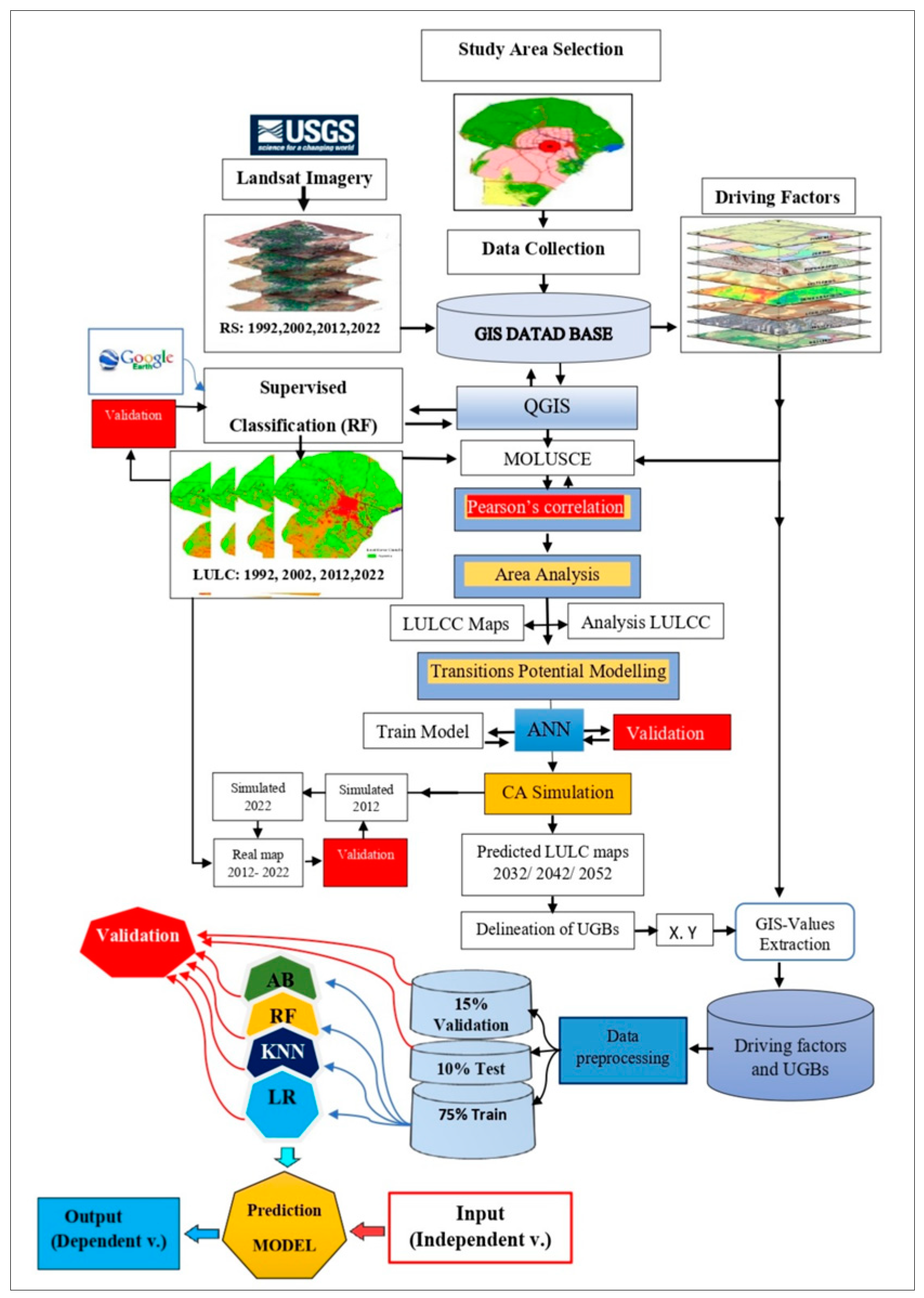
3. Materials and Methods
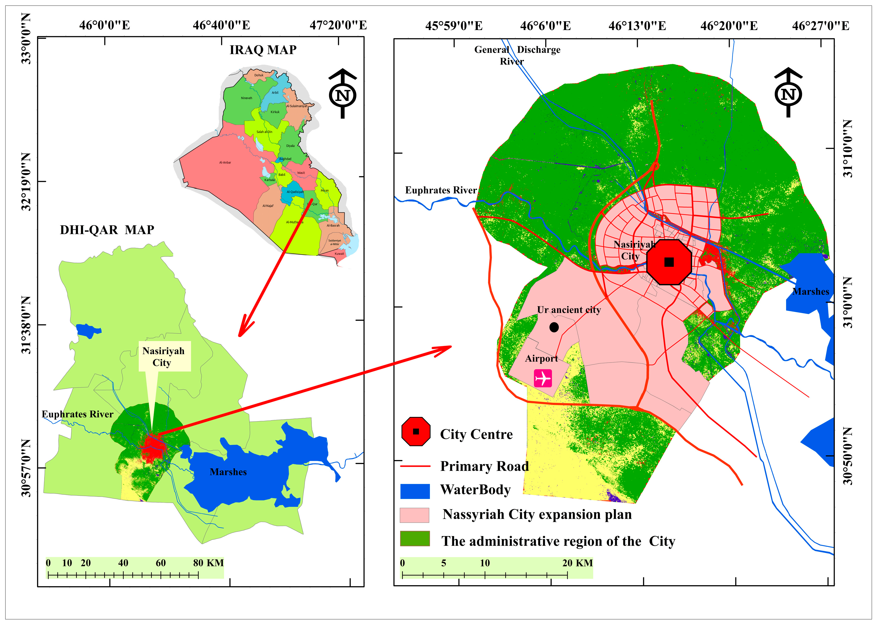
The practical basis of this study depended on the capabilities of ML algorithms to develop a land use simulation technique. Thus, this study proposed a simple, novel technique to improve spatial decisions made by optimisation land use techniques that seek optimal sites for various human activities. Several techniques were applied to achieve this goal: (1) Nasiriyah City, Iraq was chosen as the study area; (2) Landsat images for three periods, i.e., 1992, 2002, 2012 and 2022, were downloaded; (3) the supervised classification technique using RF was applied to classify Landsat images for the years 1992, 2002, 2012 and 2022; (4) the ANN-CA simulation technique was used to predict the city expansion for the next three decades (2032, 2042 and 2052); (5) the UGB technique was delineated using simulated maps; and (5) a dataset model was generated using UGBs to train ML algorithms on urban-growth trends. Figure 1 shows the overall flowchart of the methodology.

3.1. Study Area

The administrative region of Nasiriyah City, South Iraq was selected as a case study to predict the urban growth of the city (Figure 2). The area is located at 31°16′00′′ N–30°47′00′′ N, 46°00′00′′ E–46°28′00′′ E. The region is 145,000 ha, of which 46,000 ha was assigned as the future expansion of Nasiriyah City. This region has historical importance because it includes the archaeological ruins of Ur Ziggurat (4000 BCE). According to the local census of the year 2021, the population is more than 720,000. Most residents are affected by the remnants of wars occurring in the 1990s and 2000s. In addition, they have suffered from the severe effects of pollution. In the future, these pollution sites may be surrounded by urban communities driven by rapid urban growth, a rising population, economic activities and uncontrolled urbanisation. Therefore, predicting urban growth is useful for decision makers of this city and also other cities worldwide.

3.2. RS and Data Collection

LULC classification is generally based on RS images that support the major research themes regarding global environmental and climate changes. Two major categories of data were collected in this work: Landsat images and variable factors. Multispectral Landsat TM and OLI aerial imagery covering the entire research region for the years 1992, 2002, 2012 and 2022 were obtained from the US Geological Survey (USGS) website. To ensure integrity, all Landsat imagery from the same or nearby dates were used, and the highest overcast threshold was set at 5% throughout the image downloading procedure to acquire images with extremely minimal cloudiness or cloud-free images [37]. Driving force data included DEM, S, PMR, PCC, PWP, PSN, PR, PD and GDP, which were adopted as driving factors in this work; they were converted into raster layers for modelling reasons. Table 2 lists the collected data.

3.3. Method

3.3.1. GIS-Based Classification of Landsat Images Using RF

In this work, supervised classification with RF was used to classify Landsat images from the years 1992–2002, 2002–2012 and 2022. This process included several steps that were divided into three main stages: generating training samples, training the algorithm and developing the prediction model (classification maps). To generate accurate training samples, on the one hand, band combination was applied to generate true-colour composites and a false-colour composite for each Landsat image of four different land use classes (vegetation, bare land, waterbodies and urban); on the other hand, a sufficient and equal number of training plots for each class were carefully selected to acquire the most realistic land cover coverage. This was accomplished with the assistance of ancillary information platforms, such as Google Earth, to aid in the understanding of geographical characteristics [42,43]. In the training algorithm stage, each Landsat image and its corresponding training samples were defined to train the RF algorithm. The percentage of the training model was set as 70%. After making sure that values of overall accuracy and kappa were perfect, the LULC classification stage was intitated. During this stage, the final LULC maps for the years 1992, 2002, 2012 and 2022 were produced with four classes. For the accuracy assessment, the semi-automatic classification plugin (SCP) technique in QGIS was used to validate LULC classifications based on reference layers (ground truth).

3.3.2. Applying the ANN-CA Technique to Predict Urban Growth

The QGIS 2.18 program and MOLUSCE plugin were utilised [11]. In addition to the CA strategy, the MOLUSCE plugin included four forecasting methods: ANN, multicriteria evaluation, weights of evidence and LR [12]. ANN and CA were integrated in this work to analyse the LULCC of the study area for the period of 1992–2022 and to predict LULCCs for 2032, 2042 and 2052. Several independent variables were used for this experiment: P, GDP, DEM, S, PMR, PCC, PWP, PSN and PR. The MOLUSCE plugin provided several well-known techniques to assess the relationship between LULCC and independent variables. In this step, Pearson’s correlation was applied because it is the most used method for fuzzy numbers. It was adopted to check the degree of multicollinearity among independent variables; the results show that all driving factors are adequate for future land cover simulations, except for three independent variables, i.e., elevation, PD and GDP, due to the level of multicollinearity. Change analysis and transition potential modelling for the years 1992–2022 made it possible to prepare a simulation for city expansion growth for the years 2032, 2042 and 2050. Therefore, spatiotemporal changes, as well as the LULC transition between research periods (1992–2002, 2002–2012 and 2012–2022) were computed, and three LULCC maps were created. Furthermore, transition potential modelling was generated using the ANN. To prepare for the simulation process, several parameters, such as iteration value, number of hidden layers and learning rate, must be determined. The primary task was to train ANN and choose appropriate parameter values using empirical data; thus, empirical data were used to calibrate CA models via repeated runs of the same model with various parameter combinations to determine optimal parameter values. Once sufficient model validation results were achieved, the following parameters were selected whilst forecasting: 1000 iterations, a neighbourhood value of 3 pixels, a learning rate of 0.001, hidden layer of 10 and 0.05 momentum. In the simulation process, CA was applied to simulate the LULCC of 2012 by inputting the LULC values for 1992 and 2002, whereas the LULCC in 2012–2022 was used to simulate the map of year 2022. The MOLUSCE plugin provides a kappa validation approach and a comparison of real and simulated LULC maps to verify the model and prediction accuracy [11]. After obtaining good standard evaluation results, the LULC maps for years 2012 and 2022 were used in the CA technique to predict the LULC for the year 2032. In addition, the LULCs for years 2002 and 2022 were applied to simulate the LULCs for year 2042. Furthermore, the predicted maps for 2032 and 2042 were utilised to predict the LULC for year 2052.

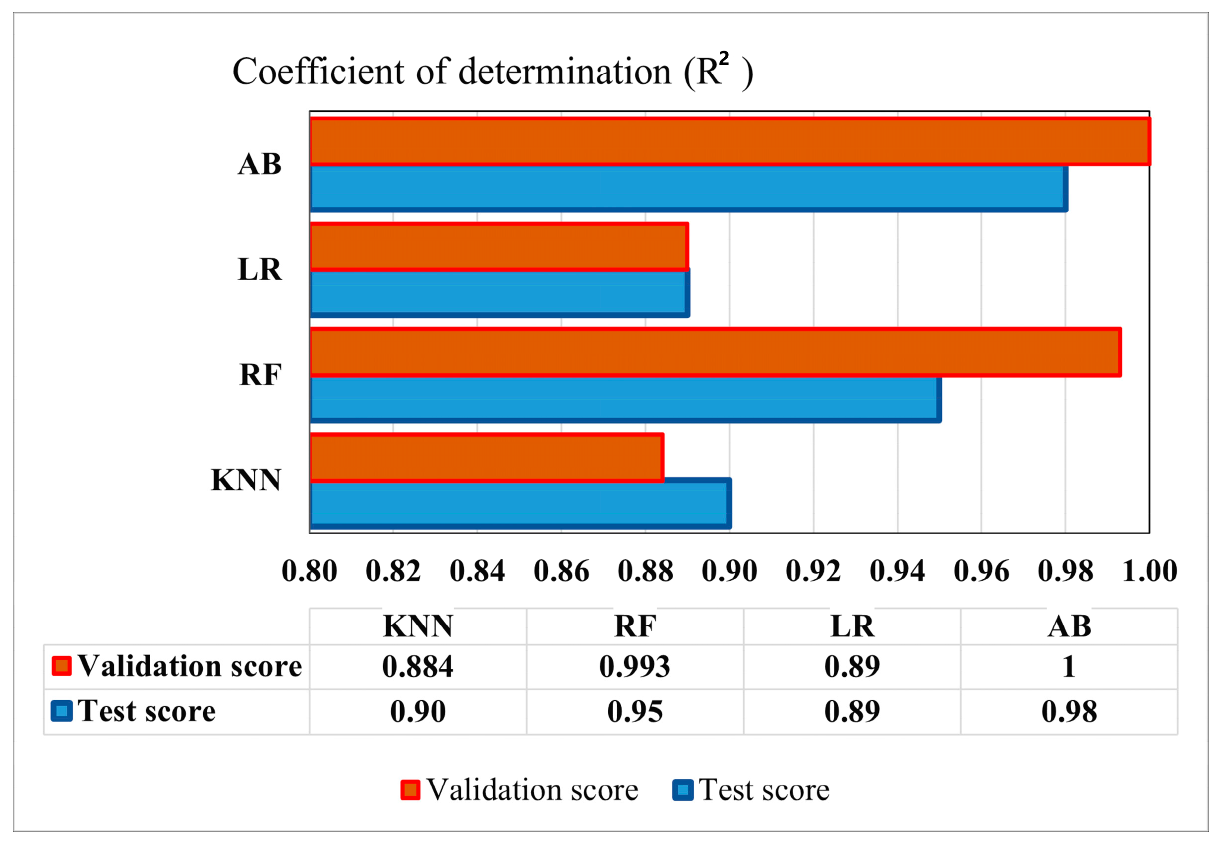
3.3.3. Structuring the Training ML Model

In this stage, a simple urban growth prediction technique was developed. Firstly, the results of the ANN-CA technique were used to delineate the UGB lines for the years 2022, 2032, 2042 and 2052, and train an ensemble of ML algorithms on the urban growth trends. Each polyline of UGBs was converted to point shapefile with equal distances, whereas the city centre was defined as the base point of the UGBs. Then, the technique of extracting multivalues from points in GIS was used to extract the values of the variable layers. The six values were used as independent variables in the dataset model, whereas the yearly date of urban growth was selected as the dependent variable (outcome). The dataset was subjected to several types of data preprocessing, the most important of which were handling missing values, removing outliers and extreme values, dealing with imbalanced classification issues using the synthetic minority oversampling technique and applying the feature reduction process to exclude redundant independent variables using multicollinearity analysis as a final check. In the multicollinearity analysis process, the values of the tolerance and variance inflation factor (VIF) were calculated as the final check of the level of multicollinearity among independent variables using SPSS software. The analysis revealed that the level of correlation among the seven independent variables is within an acceptable range, the tolerance values are greater than 0.1 (0.25 to 0.83) and the VIF are less than 10 (1.20 to 4.02). Then, a data sampler tool was used to divide the dataset into three parts: 70% training samples, 15% validating samples for unbiased evaluation of the model and 10% testing samples for evaluation of the model. Once the ML algorithms were run, the performance metrics for each model were measured to evaluate the goodness of fit of the different ML models; consequently, the result analysis supports the selection of four suitable algorithms among different ML models, namely, RF, KNN, AB and LR. In addition to this typical method, different algorithms were tested on validation datasets to select suitable ML algorithms for the model dataset, and several other factors were considered, the most important of which were interpretability, dataset size, data linearity, data format and training and prediction times.
1.
RF
RF has a high interpretability of relationship between independent and dependent variables. In contrast to the other algorithms, RF can evaluate and handle numerous variables, including regression, classification and feature extraction [44]. Most previous studies indicated that the RF algorithm can handle high data multidimensionality and is rapid and sensitive to overfitting [39]. It requires less time for training and prediction. In addition, it is the most suitable ML for LULCC. Although this model has high fitting and generalisation capabilities, its basic principle is simple to grasp [45]. It is multiple decision trees that compose the integrated ML model [46]. In RF, the tree predictors are mixed, with each tree relying on separately collected values from a random vector and sharing a common distribution; thus, RF improves prediction accuracy [47,48]. In this work, the parameters were as follows: the number of trees was 10, the minimum sample was 5 and the limit depth of individual trees was 15.
2.
KNN
Although KNN works effectively with large amounts of data and numerous variables, it offers indicators that are simple to understand. To fit the dataset, KNN uses an extremely simple ML technique [49]. Given its simplicity and effectiveness, KNN is a good nonparametric ML algorithm that is used in various pattern recognition applications [50]. KNN-based approaches use Euclidean distance to compute the match of a training and testing model; subsequently, KNN is identified on the basis of computed correlations, defining the output label of the testing model, that is, the most votes amongst the k-neighbours. [51]. In addtion, it is capable of rapid training and prediction. In this study, the KNN was set as follows: the number of neighbours was 5 and the metrics were Euclidean.
3.
AB
AB is an ensemble learning algorithm that builds a strong classifier from a series of weak learners and minimises sensitivity to noisy input [52]. It has a high standardisation ability, efficient speed and minimal application complexity [53,54]. It applies a weight to each variable in the training dataset in a repeated fashion [55]. The sample weights are changed until the model meets its prediction accuracy criteria or the maximum number of iterations is attained [56]. The data samples are trained in each iteration on the basis of the classifier’s different weights to reduce training failures and provide accurate predictions [57]. It is most effective when used to boost DT performance on binary classification problems [58]. In this work, the parameters were as follows: the function was linear regression; the fixed seed for the random generator was 3.
4.
LR
Given that the dataset in this experiment is almost linear, linear regression is an appropriate choice. It uses a linear formula to obtain the best fit line (straight line) for an issue, allowing visualisation and predicting the dependent variables’ output based on Formula 1. In addition, conventional ML approaches, such as logistic regression, may generate rapid predictions. Furthermore, LR is a simple yet effective supervised learning technique. A target variable (dependent variable) is predicted by LR using one or more feature variables (independent variables). The target value is often a continuous, real-value variable [59]. Given that the regression technique can predict continuous outcomes for a long time, this study proposed to forecast a city expansion for a long time. Regression ML can investigate the relationship between independent variables (IVs) and a dependent variable (DV) to predict the spatiotemporal of UGBs in the study area. LR may be beneficial not just for detecting patterns in experimental data, but also for benchmarking and testing new analytic approaches, particularly those that are novel or unfamiliar [60]. The logistic function is used by the LR model to establish a relationship between land use class (a dependent variable) and its driving force (independent variables), making it a viable tool for mining CA conversion rules [18,61]. In this work, the parameters were as follows: the ridge regression (L1) was 0.0001 and Lasso regression (L2) was 0.50:0.50.
Y i = f ( X i , B ) + e i ,
where Yi represents the outcome variable, f represents a function, Xi represents the attribute, B represents unknown values and e represents standard errors.

3.3.4. Spatial Applicability of the Novel ML Model

To apply the novel technique spatially, a sample of six polluting factories was selected to predict UGBs and validate the buffer zone. According to Iraqi Environment Standards (IES) (specifically, number 3-2011) which has been adopted by the Iraqi Ministry of Environment [62], buffer zones must be left between UGBs and pollution-causing projects, as shown in Table 3, to protect urban communities from harmful gas emissions. Similar to the previous section (structuring the training ML), the seven values of driving factors were extracted for each specific location of the six selected projects on the basis of their coordinates by using the GIS analysis technique to generate the prediction model. The model was included from seven attributes (driving factors) as independent variables, whereas the dependent variable was the yearly date of UBG, which is an unknown value that would to be predicted by running trained ML algorithms.

3.4. Validation

In the classification stage, the trained model of classification was validated by the RF algorithm on the basis of two evaluation metrics, namely, overall accuracy (OC) and kappa coefficient. Equations (2) and (3) show the calculation method of OC and kappa [9,36,63]. Furthermore, the final classification maps for the years 1992, 2002, 2012 and 2022 were validated by the SCP technique. In the following stage, i.e., LULC prediction, the simulated maps for the years 2012 and 2022 were validated on the basis of the real maps for the same years.
O C = T C . P T S . P × 100 ,
where OC denotes overall accuracy, TC.P is the total number of properly identified pixels and TS.P is the total number of sample pixels.
k a p p a   c o e f f i c i e n t = O . A C . A 1 C . A ,
where O.A is the overall accuracy and C.A is the chance agreement.
In the model prediction stage, the evaluation process of the goodness of fit of regression ML models was applied, and several metrics were measured each time the model was run. As a result, after running the four ML algorithms, i.e., RF, KNN, AB and LR, the following performance metrics were achieved for each model: coefficient of determination (R2), mean absolute error (MAE) and root-mean-squared error (RMSE) based on Equations (4)–(6) [64,65]. In a regression ML model, R2 reflects the fraction of the dependent variable’s variation that has been explained by the model’s independent variables [66]. Furthermore, for each ML model, MAE and RMSE describe the divergence between actual and observed data points and anticipated data points [67]. For validation, 15% of the dataset was used as a validation set for unbiased evaluation to perform model selection; in addition, 10% of the testing set was applied to determine if the final model chosen by the validation set can adapt well to new, unseen data.
R 2 = 1 i = 1 n ( y i y ^ i ) 2 i = 1 n ( y i y ¯ i ) 2
R M S E = i = 1 n ( y i y ^ i ) 2 n
M A E = 1 n i = o n 1 | y i y ^ i |
where yi is the equivalent real value, y ^ i denotes the predicted value of the i-the sample and n denotes the total number of samples or errors.

4. Result and Analysis

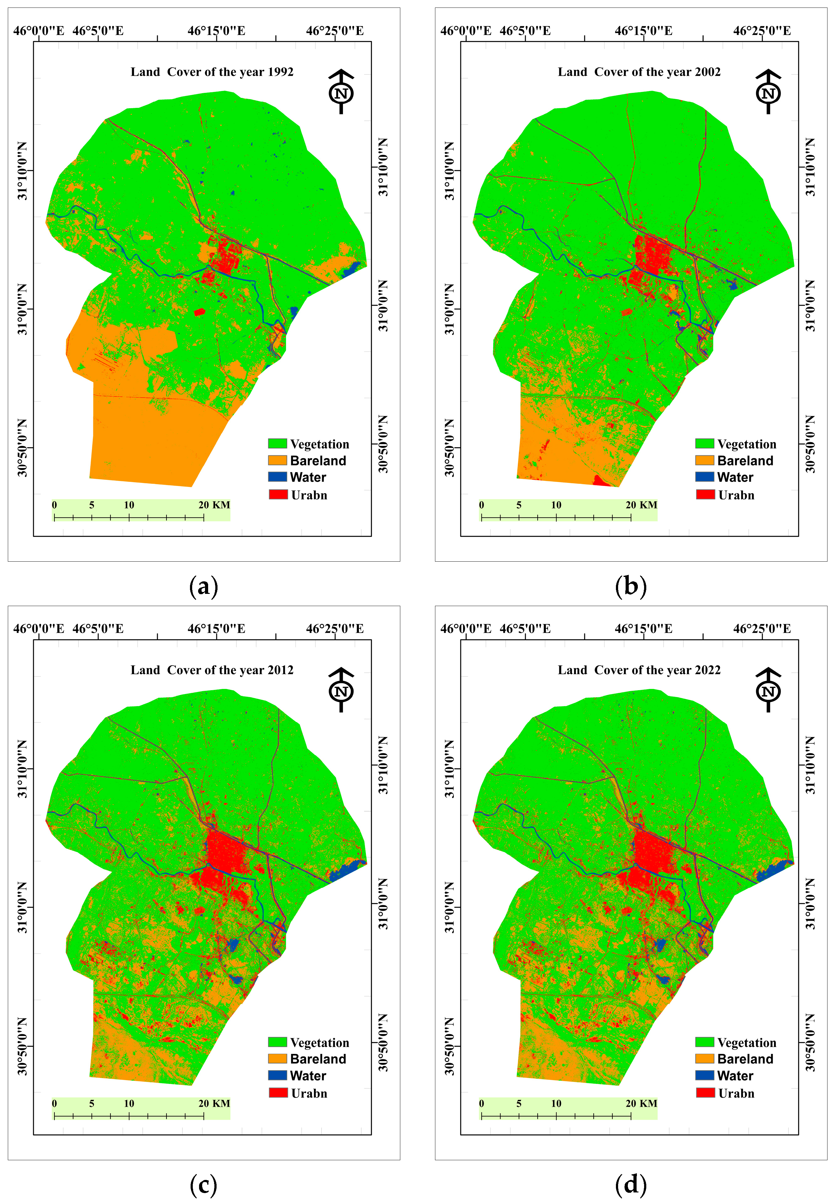
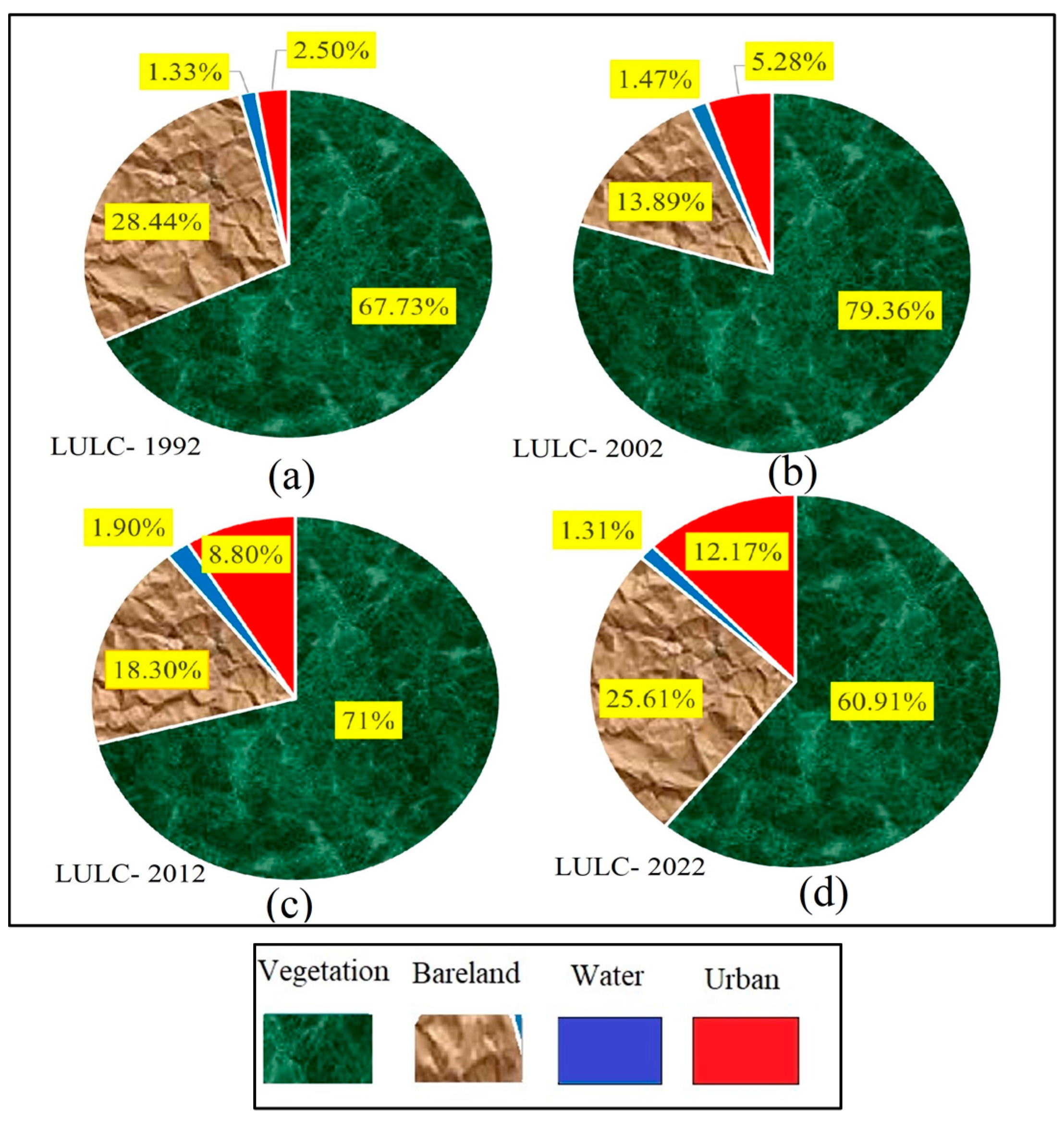
4.1. Classification of Landsat Image Results

The supervised classification techniques (RF in QGIS) classified the Landsat images from 1992, 2002, 2012 and 2022 with high accuracy. The minimum of kappa values was 88%, and the minimum OA was 93%. The outcomes indicate that the observed LULCC are predominantly rapid across Nasiriyah City from the year 1992 to 2020 and turned into urban areas at the expense of other land use classes. The urban area ratio increased by about 10%, i.e., from 2.5% in the year 1992 to 12.17% in 2022. The urban sprawl was at the expense of vegetation (6.82%), bare land (2.83%) and water (0.02%), as shown in Figure 3 and Figure 4. This change was a result of migration from rural areas to the city, in addition to the fact that the study area is the economic centre of about 2 million people.

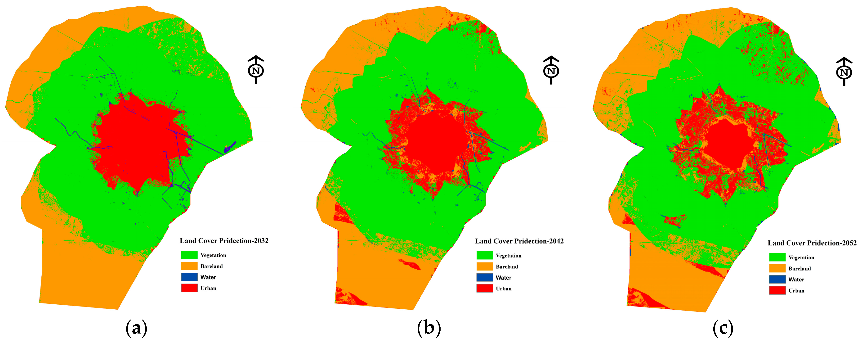
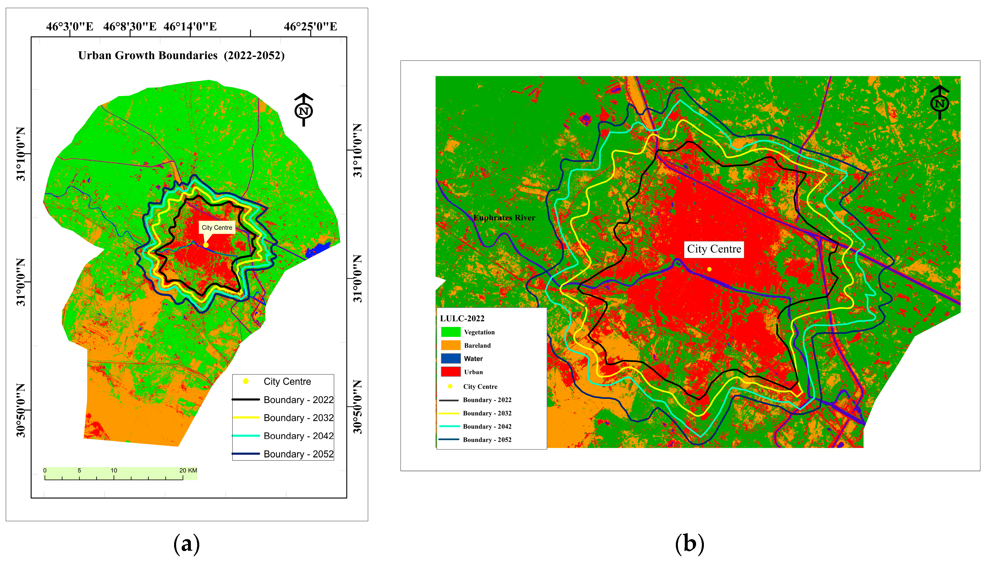
4.2. Prediction Result of Urban Growth

The results reveal that the accuracy of performance of ANN-CA is an ‘almost perfect agreement’, with an overall kappa value of 90.3% and 80.2% for the simulated maps of years 2012 and 2022, respectively, based on the maps of the same years. The prediction result for the following three decades (2032, 2042 and 2052) supports the historical trend of urbanisation at the expense of considerable quantities of vegetation area. The urban area ratio of the general region increased by about 7.92 %, i.e., from 12.17% in the year 2022 to 20.09% in 2052. Urban sprawl occurred at the expense of vegetation (7.63%) and water (0.29%). Meanwhile, the city would be expanded by 34%, 25% and 19% by the years 2032, 2042 and 2052, respectively, as shown in Figure 5. These results were required for delineating UGB lines for the years 2022, 2032, 2042 and 2052 to train the ensemble of ML algorithms on the urban growth trends, as shown in Figure 6.

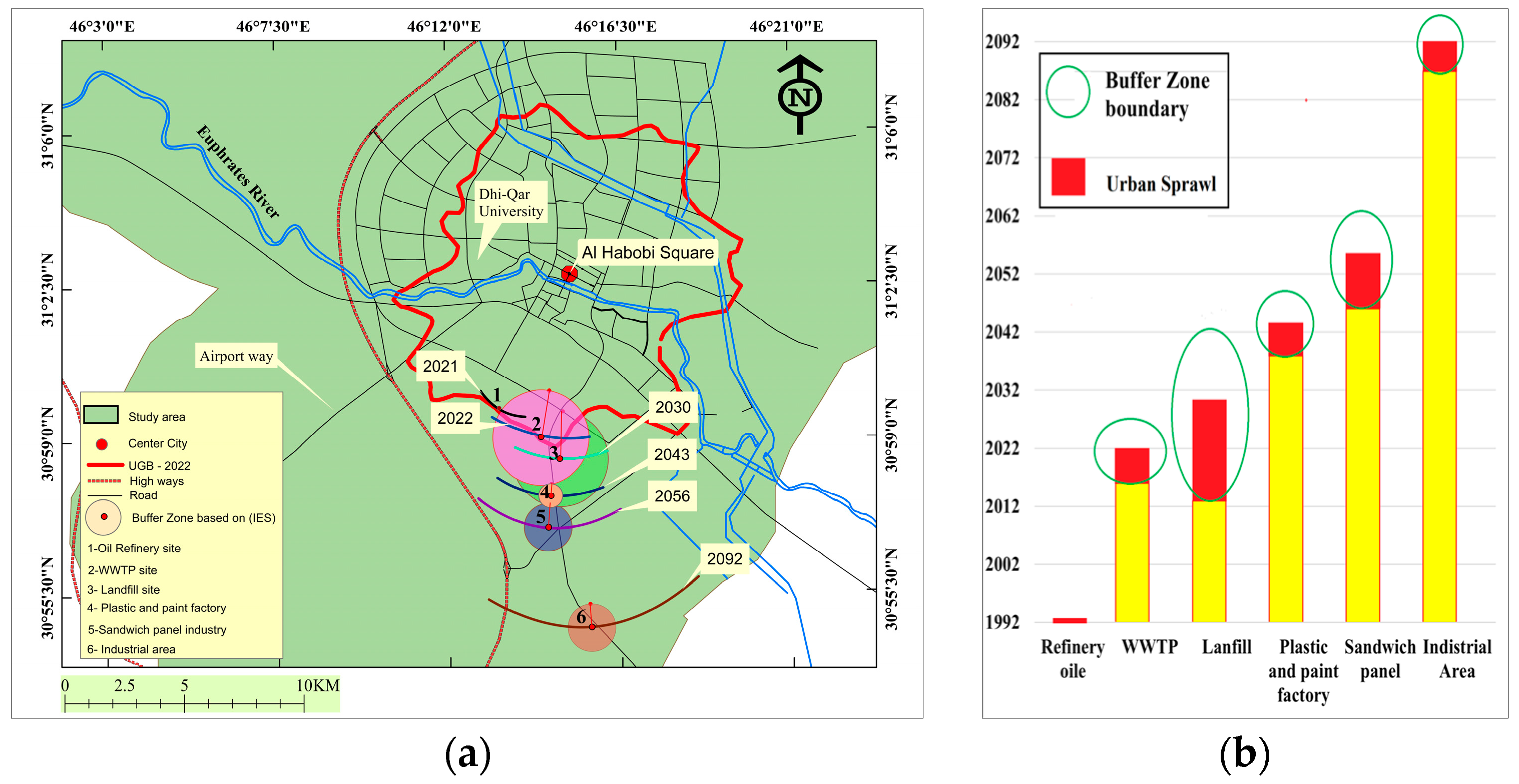
4.3. Result of the Spatial Applicability of the Novel ML Model

The results of spatial applicability confirm that the novel ML model is effective, according to the validation metrics that were measured by the four ML algorithms. On the one hand, the test score result reveals that the values for the coefficient of determination (R2) are 98%, 96%, 90% and 89%, which were measured by AB, RF, KNN and LR, respectively. On the other hand, the validation score result reveals that the values of R2 are 100%, 99%, 89% and 88%, which were validated by AB, RF, LR and KNN, respectively. In addition, the predicted results proven by the novel approach are efficient in supporting decision systems regarding land use optimisation, especially selecting pollution-causing project sites. It accurately determined the date of the intersection of UGBs with the buffer zone of the sample of the pollution-causing projects that were selected in this work. The results predicted are as follows:
5.
Project No. 1 (oil refinery)
UGB already reached the location centre in the year 2021, indicating that the location centre of the oil refinery violates IES. According to IES, the buffer zone between UGBs and an oil refinery must be 10 km to protect the urban community from gas emissions.
6.
Project No. 2 (WWTP)
UGB was intersected with a buffer zone around the WWTP in the year 2016 and will reach its location centre in the year 2022. Although the project is presently under construction, it violates the IES, which enforces a 2 km buffer zone.
7.
Project No. 3 (landfill site)
UGB intersected the buffer zone around the landfill site in the year 2013, and it will reach the location centre by the year 2030. Therefore, the location of this project must be moved in accordance with the IES, which enforces 2 km as a buffer zone from the UGB. Based on local environmental reports, the majority of Nasiriyah City residents suffer from the bad smell and smoke released from this site.
8.
Project No. 4 (plastic and paint factory)
UGB will intersect with the buffer zone around the factory in the year 2038, and it will reach the location centre by the year 2043. The factory must be moved to a farther site by the year 2038 due to IES, which enforces 500 m as a buffer zone from the UGB.
9.
Project No. 5 (sandwich panel factories)
UGB will intersect with the buffer zone around the factory in the year 2046, and it will reach the location centre by the year 2056. The factory must be moved by 2046 due to IES, which enforces 1 km as a buffer zone of from the UGB.
10.
Project No. 6 (industrial area)
UGB will intersect with the buffer zone around the factory in the year 2087, and it will reach the location centre by the year 2092. Its location is suitable based on IES, which enforces 1 km as a buffer zone of from the UGB. Figure 7 shows the prediction results regarding the sample of the pollution-causing projects that were selected in this study.

5. Validation Result

In this work, the validation results reveal that the ML model was run with high accuracy, and the performance indexes were measured to validate the sequential results of each stage. The indexes indicated that the performance of the techniques used in this study was almost perfect. Firstly, the accuracy performance of Landsat image classification was validated with high accuracy in the two steps, i.e., model training using RF and final LULC classification using SCP in QGIS, as listed in Table 3. Secondly, to calibrate the ANN-CA technique, the LULCs for 2012 and 2022 were simulated; thus, the accuracy of the simulation maps was validated on the basis of the real maps of the same years and was in ‘almost perfect agreement’, as listed in Table 4. Finally, in predicting the UGB stage, the trained model was validated using the four ML algorithms, i.e., RF, KNN, AB and LR, using the testing set (10%) and validation set (15%) via a confusion matrix test, as shown in Figure 8.

6. Discussion

The urban communities near pollution-causing factories are exposed to risks of environmental pollution [1]. To mitigate possible counteractions, substantial research has proposed appropriate solutions, including many land use optimisation methods. The most common methods of spatial optimisation are GIS-MCDM and the integration of GIS and ML models along with RS data [5,46,62,68,69,70,71,72,73,74,75,76,77,78,79,80,81,82,83,84,85,86,87]. However, in both approaches, the spatial decision is made on the basis of multicriteria, most of which are spatial dynamic factors; however, the practical principle of these approaches does not consider dynamic LULCC due to urban growth. Consequently, a city would likely sprawl close to the pollution-causing projects that were selected, causing considerable effects on sustainability. Therefore, a novel technique was proposed in this study to solve the abovementioned problem.
The findings of this work reveal that the novel approach is highly efficient for the proactive prediction of potential long-term environmental effects, as well as the detection of environmental impacts at present. The overall result shows that the Nasiriyah City expansion (the study area) is haphazard and unplanned, resulting in disastrous effects on urban and natural systems. The urban sprawl would continue towards the area on which built or proposed industrial projects violate local environmental standards (IESs), which aim to protect urban communities from environmental pollution. The analysis result shows that the urban area ratio increases by about 10%, i.e., from 2.5% in the year 1992 to 12.2% in 2022. This change was at the expense of vegetation (6.7%), bare land (2.84%) and water (0.02%). Furthermore, the prediction results reveal that the city will expand by 34%, 25% and 19 % by the years 2032, 2042 and 2052, respectively. In addition, the land use assessment result for the sixth site confirms that the novel technique can forecast city expansion until 2092. It is one of the advantages that the present study seeks. The validation results confirm that the performance of the novel ML model is effective, according to the validation metrics that were measured by the four ML algorithms, i.e., AB, RF, LR and KNN. The coefficient of determination (R2) values ranged from 88% to 100%.
In contrast to conventional and modern approaches of LULC optimisation and simulation, the novel technique can effectively validate and support the decision-making process regarding long-term land use planning. Nevertheless, their advantages cannot be underestimated, although their results are often associated with uncertainty [68,69,70,71,72,73,74,75,76,81,82,83,84,85,86,87]. The practical principle of almost all land use optimisation methods is similar, that is, their outcome is driven by multicriteria, which contribute different factors to the decision-making process. However, most of these criteria are dynamic spatial factors that change over time due to the impact of urban sprawl [8,88]. Given that this change is neglected when using land use optimisation techniques, the decisions that are made on the basis of multicriteria would be converted from strong to weak over time. To overcome this issue, simulation techniques could be applied because these techniques provide a comprehensive perspective of current and future development opportunities [11].
Although ANN-CA is the most effective technique, which has been recently commended by many scholars [7,8], integrating it with land use optimisation approaches to make a sustainable decision regarding a suitable site for various activities is complex. It requires multiple operations that must be conducted in sequential steps when a suitable location for a specific activity is chosen. Whilst most strategic industrial projects, such as oil refineries, power energy electricity and WWTP, are designed to work for multiple decades, all prediction techniques are restricted to predict over three decades with acceptable accuracy. To bridge these gaps, the novel approach based on ML and GIS was developed. The results of this study confirm that using this novel technique can avoid the probability of incorrect decisions that cost a high amount when their consequences are corrected.
The advantages and disadvantages of the proposed approach are arguable. To what extent the novel technique may be used to forecast urban sprawl in other cities has yet to be answered. Each city has spatial properties, i.e., area of the city, distance from the city centre to UGB, design of roads and proximity of the rivers from built-up areas. The novel model predicts UGB on the basis of these properties and the historical trend of LULCC that can be obtained from the archive of Landsat images. Therefore, the model can be applied to another city with its own spatial properties. Another argument that could spark discussion is that although this novel approach can monitor urban growth with high accuracy, the other factors that contribute to the selection of optimal sites are neglected. The main aim of developing this approach was to overcome the limitations of the land use optimisation technique. This novel technique can be applied before using either GIS-MCDM or GIS-ML to exclude the sites that would be covered by city expansion in the future.
The novel technique can discover planning problems of projects that were built in the past, and it can predict potential environmental problems of projects under construction and even the proposed location of planning projects. Therefore, it can be a DST for land use optimisation, especially in selecting sites of pollution-causing projects. This technique is necessary for scholars and urban planners who are interested in sustainable development goals (SDGs).

7. Conclusions and Future Implications

Although advanced techniques have been involved in and integrated with conventional land use optimisation approaches, dynamic LULCCs are still neglected as crucial driving forces. Thus, this study focused on developing a novel technique that considers the dynamic LULCCs to support decision-making processes regarding SDGs. To this end, three main processes were applied, namely, a supervised classification process using RF, prediction of urban growth using a hybrid method of ANN-CA and development of ensemble ML models using four ML algorithms (i.e., KNN, RF, AB and LR), to predict long-term UGBs. In addition, the integration of GIS and RS played a critical role in developing the novel technique. The novel technique was applied to the sample of six pollution-causing factories, and the results confirm that the technique is a practical method that should be integrated with MCDM to make wise decisions and validate previous decisions. On the one hand, the results reveal that five sites were constructed at the wrong location due to neglected LULCC dynamics when site-selection decisions were made; this mistake produced disastrous effects on the urban and natural systems. On the other hand, the assessment result for the sixth site demonstrates that the new method can forecast UGB expansion until 2092, which is one of the reasons that the technique was developed. Consequently, the novel technique showed long-term potential environmental effects and detected the environmental impacts at present due to urban sprawl. In addition, the result shows that the urban area ratio increases by about 10%, i.e., from 2.5% in the year 1992 to 12.2% in 2022. This change was at the expense of vegetation (6.7%), bare land (2.84%) and water (0.02%). Furthermore, the prediction results show that the historic trend of LULCC will continue for the next three decades. Urban sprawl would expand by 34%, 25% and 19% by the years 2032, 2042 and 2052, respectively. Therefore, this novel technique can be integrated with GIS-MCDM or GIS-ML to exclude the sites that would be covered by the future city expansion. It can be a DST for land use optimisation, especially in selecting sites for pollution-causing projects. However, the selection of relevant driving factors was the major shortcoming of this work. It requires encouraging the public to overcome the bias associated with experts’ opinions. Further studies should be conducted to highlight another critical issue, which is the interaction between urban sprawl and the efficiency of urban water supply.

Author Contributions

Conceptualization, Sadeq Khaleefah Hanoon and Ahmad Fikri Abdullah; Methodology, Sadeq Khaleefah Hanoon; Software, Sadeq Khaleefah Hanoon; Validation, Sadeq Khaleefah Hanoon, Ahmad Fikri Abdullah, Helmi Z. M. Shafri and Aimrun Wayayok; Formal analysis, Sadeq Khaleefah Hanoon; Investigation, Sadeq Khaleefah Hanoon and Ahmad Fikri Abdullah; Resources, Sadeq Khaleefah Hanoon; Data curation, Sadeq Khaleefah Hanoon; Writing – original draft, Sadeq Khaleefah Hanoon; Writing – review & editing, Sadeq Khaleefah Hanoon and Ahmad Fikri Abdullah; Visualization, Sadeq Khaleefah Hanoon; Supervision, Sadeq Khaleefah Hanoon, Ahmad Fikri Abdullah, Helmi Z. M. Shafri and Aimrun Wayayok. All authors have read and agreed to the published version of the manuscript.

Funding

This research received no external funding.

Institutional Review Board Statement

Not applicable.

Informed Consent Statement

Not applicable.

Data Availability Statement

All data are reported in this paper.

Conflicts of Interest

The authors declare no conflict of interest.

References

  1. Bseibsu, A.; Madhuranthakam, C.M.R.; Yetilmezsoy, K.; Almansoori, A.; Elkamel, A. Numerical Simulation of Dispersion Patterns and Air Emissions for Optimal Location of New Industries Accounting for Environmental Risks. Pollutants 2022, 2, 444–461. [Google Scholar] [CrossRef]
  2. Aniah, P.; Bawakyillenuo, S.; Codjoe, S.N.A.; Dzanku, F.M. Land use and land cover change detection and prediction based on CA-Markov chain in the savannah ecological zone of Ghana. Environ. Challenges 2023, 10, 100664. [Google Scholar] [CrossRef]
  3. Ghosh, S.; Das Chatterjee, N.; Dinda, S. Urban ecological security assessment and forecasting using integrated DEMATEL-ANP and CA-Markov models: A case study on Kolkata Metropolitan Area, India. Sustain. Cities Soc. 2021, 68, 102773. [Google Scholar] [CrossRef]
  4. Taherdoost, H.; Madanchian, M. Multi-Criteria Decision Making (MCDM) Methods and Concepts. Encyclopedia 2023, 3, 77–87. [Google Scholar] [CrossRef]
  5. Hanoon, S.K.; Abdullah, A.F.; Shafri, H.Z.M.; Wayayok, A. A Novel Approach Based on Machine Learning and Public Engagement to Predict Water-Scarcity Risk in Urban Areas. ISPRS Int. J. Geo-Inf. 2022, 11, 606. [Google Scholar] [CrossRef]
  6. Chen, Z.; Huang, M.; Zhu, D.; Altan, O. Integrating Remote Sensing and a Markov-FLUS Model to Simulate Future Land Use Changes in Hokkaido, Japan. Remote Sens. 2021, 13, 2621. [Google Scholar] [CrossRef]
  7. Tripathy, P.; Kumar, A. Monitoring and modelling spatio-temporal urban growth of Delhi using Cellular Automata and geoinformatics. Cities 2019, 90, 52–63. [Google Scholar] [CrossRef]
  8. Saha, T.K.; Pal, S.; Sarkar, R. Prediction of wetland area and depth using linear regression model and artificial neural network based cellular automata. Ecol. Inform. 2021, 62, 101272. [Google Scholar] [CrossRef]
  9. Kamaraj, M.; Rangarajan, S. Predicting the future land use and land cover changes for Bhavani basin, Tamil Nadu, India, using QGIS MOLUSCE plugin. Environ. Sci. Pollut. Res. 2022, 29, 86337–86348. [Google Scholar] [CrossRef]
  10. Wang, Q.; Wang, H. Spatiotemporal dynamics and evolution relationships between land-use/land cover change and landscape pattern in response to rapid urban sprawl process: A case study in Wuhan, China. Ecol. Eng. 2022, 182, 106716. [Google Scholar] [CrossRef]
  11. Muhammad, R.; Zhang, W.; Abbas, Z.; Guo, F.; Gwiazdzinski, L. Spatiotemporal Change Analysis and Prediction of Future Land Use and Land Cover Changes Using QGIS MOLUSCE Plugin and Remote Sensing Big Data: A Case Study of Linyi, China. Land 2022, 11, 419. [Google Scholar] [CrossRef]
  12. Wang, P.; Huang, X.; Mango, J.; Zhang, D.; Xu, D.; Li, X. A Hybrid Population Distribution Prediction Approach Integrating LSTM and CA Models with Micro-Spatiotemporal Granularity: A Case Study of Chongming District, Shanghai. ISPRS Int. J. Geo-Inf. 2021, 10, 544. [Google Scholar] [CrossRef]
  13. Khan, A.; Sudheer, M. Machine learning-based monitoring and modeling for spatio-temporal urban growth of Islamabad. Egypt. J. Remote Sens. Space Sci. 2022, 25, 541–550. [Google Scholar] [CrossRef]
  14. Littidej, P.; Uttha, T.; Pumhirunroj, B. Spatial Predictive Modeling of the Burning of Sugarcane Plots in Northeast Thailand with Selection of Factor Sets Using a GWR Model and Machine Learning Based on an ANN-CA. Symmetry 2022, 14, 1989. [Google Scholar] [CrossRef]
  15. Lin, J.; Li, X.; Wen, Y.; He, P. Modeling urban land-use changes using a landscape-driven patch-based cellular automaton (LP-CA). Cities 2023, 132, 103906. [Google Scholar] [CrossRef]
  16. Mitsova, D.; Shuster, W.; Wang, X. A cellular automata model of land cover change to integrate urban growth with open space conservation. Landsc. Urban Plan. 2011, 99, 141–153. [Google Scholar] [CrossRef]
  17. Küçük Matcı, D.; Çömert, R.; Avdan, U. Analyzing and Predicting Spatiotemporal Urban Sprawl in Eskişehir Using Remote Sensing Data. J. Indian Soc. Remote Sens. 2022, 50, 923–936. [Google Scholar] [CrossRef]
  18. Mustafa, A.; Rienow, A.; Saadi, I.; Cools, M.; Teller, J. Comparing support vector machines with logistic regression for calibrating cellular automata land use change models. Eur. J. Remote Sens. 2018, 51, 391–401. [Google Scholar] [CrossRef]
  19. Xu, Q.; Wang, Q.; Liu, J.; Liang, H. Simulation of Land-Use Changes Using the Partitioned ANN-CA Model and Considering the Influence of Land-Use Change Frequency. ISPRS Int. J. Geo-Inf. 2021, 10, 346. [Google Scholar] [CrossRef]
  20. Pu, R. Mapping Tree Species Using Advanced Remote Sensing Technologies: A State-of-the-Art Review and Perspective. J. Remote Sens. 2021, 2021, 9812624. [Google Scholar] [CrossRef]
  21. Rimal, B.; Zhang, L.; Keshtkar, H.; Haack, B.N.; Rijal, S.; Zhang, P. Land Use/Land Cover Dynamics and Modeling of Urban Land Expansion by the Integration of Cellular Automata and Markov Chain. ISPRS Int. J. Geo-Inf. 2018, 7, 154. [Google Scholar] [CrossRef] [Green Version]
  22. Lai, Z.; Chen, C.; Chen, J.; Wu, Z.; Wang, F.; Li, S. Multi-Scenario Simulation of Land-Use Change and Delineation of Urban Growth Boundaries in County Area: A Case Study of Xinxing County, Guangdong Province. Land 2022, 11, 1598. [Google Scholar] [CrossRef]
  23. Liang, X.; Liu, X.; Li, X.; Chen, Y.; Tian, H.; Yao, Y. Delineating multi-scenario urban growth boundaries with a CA-based FLUS model and morphological method. Landsc. Urban Plan. 2018, 177, 47–63. [Google Scholar] [CrossRef]
  24. Jin, Y.; Li, A.; Bian, J.; Nan, X.; Lei, G. Modeling the Impact of Investment and National Planning Policies on Future Land Use Development: A Case Study for Myanmar. ISPRS Int. J. Geo-Inf. 2023, 12, 22. [Google Scholar] [CrossRef]
  25. Jin, M.; Feng, R.; Wang, L.; Yan, J. A Study of Diffusion Equation-Based Land-Use/Land-Cover Change Simulation. ISPRS Int. J. Geo-Inf. 2021, 10, 383. [Google Scholar] [CrossRef]
  26. Cui, J.; Zhu, M.; Liang, Y.; Qin, G.; Li, J.; Liu, Y. Land Use/Land Cover Change and Their Driving Factors in the Yellow River Basin of Shandong Province Based on Google Earth Engine from 2000 to 2020. ISPRS Int. J. Geo-Inf. 2022, 11, 163. [Google Scholar] [CrossRef]
  27. Navarro Cerrillo, R.M.; Rodríguez, G.P.; Rumbao, I.C.; Lara, M.Á.; Bonet, F.J.; Mesas-Carrascosa, F.J. Modeling major rural land-use changes using the gis-based cellular automata metronamica model: The case of andalusia (southern spain). ISPRS Int. J. Geo-Inf. 2020, 9, 458. [Google Scholar] [CrossRef]
  28. Megahed, Y.; Cabral, P.; Silva, J.; Caetano, M. Land Cover Mapping Analysis and Urban Growth Modelling Using Remote Sensing Techniques in Greater Cairo Region—Egypt. ISPRS Int. J. Geo-Inf. 2015, 4, 1750–1769. [Google Scholar] [CrossRef] [Green Version]
  29. Hanoon, S.K.; Abdullah, A.F.; Shafri, H.Z.M.; Wayayok, A. Using scenario modelling for adapting to urbanization and water scarcity: Towards a sustainable city in semi-arid areas. Period. Eng. Nat. Sci. (PEN) 2021, 10, 518–532. [Google Scholar] [CrossRef]
  30. Li, K.; Feng, M.; Biswas, A.; Su, H.; Niu, Y.; Cao, J. Driving Factors and Future Prediction of Land Use and Cover Change Based on Satellite Remote Sensing Data by the LCM Model: A Case Study from Gansu Province, China. Sensors 2020, 20, 2757. [Google Scholar] [CrossRef]
  31. Hu, Z.; Lo, C. Modeling urban growth in Atlanta using logistic regression. Comput. Environ. Urban Syst. 2007, 31, 667–688. [Google Scholar] [CrossRef]
  32. Wu, Q.; Li, H.-Q.; Wang, R.-S.; Paulussen, J.; He, Y.; Wang, M.; Wang, B.-H.; Wang, Z. Monitoring and predicting land use change in Beijing using remote sensing and GIS. Landsc. Urban Plan. 2006, 78, 322–333. [Google Scholar] [CrossRef]
  33. Mansour, S.; Alahmadi, M.; Atkinson, P.M.; Dewan, A. Forecasting of Built-Up Land Expansion in a Desert Urban Environment. Remote Sens. 2022, 14, 2037. [Google Scholar] [CrossRef]
  34. Traore, A.; Watanabe, T. Modeling Determinants of Urban Growth in Conakry, Guinea: A Spatial Logistic Approach. Urban Sci. 2017, 1, 12. [Google Scholar] [CrossRef] [Green Version]
  35. Yang, R.; Qin, B.; Lin, Y. Assessment of the Impact of Land Use Change on Spatial Differentiation of Landscape and Ecosystem Service Values in the Case of Study the Pearl River Delta in China. Land 2021, 10, 1219. [Google Scholar] [CrossRef]
  36. Past, A.; Land, F.; Land, U.; Kumar, P. Cellular Automata-Based Artificial Neural Network Model for Cover Dynamics. Agronomy 2022, 12, 2772. [Google Scholar]
  37. Ashwini, K.; Sil, B.S. Impacts of Land Use and Land Cover Changes on Land Surface Temperature over Cachar Region, Northeast India—A Case Study. Sustainability 2022, 14, 14087. [Google Scholar] [CrossRef]
  38. Liu, Y.; Feng, Y. Simulating the Impact of Economic and Environmental Strategies on Future Urban Growth Scenarios in Ningbo, China. Sustainability 2016, 8, 1045. [Google Scholar] [CrossRef] [Green Version]
  39. Zhang, D.; Liu, X.; Wu, X.; Yao, Y.; Wu, X.; Chen, Y. Multiple intra-urban land use simulations and driving factors analysis: A case study in Huicheng, China. GIScience Remote Sens. 2018, 56, 282–308. [Google Scholar] [CrossRef]
  40. Mengistu, T.D.; Chung, I.-M.; Kim, M.-G.; Chang, S.W.; Lee, J.E. Impacts and Implications of Land Use Land Cover Dynamics on Groundwater Recharge and Surface Runoff in East African Watershed. Water 2022, 14, 2068. [Google Scholar] [CrossRef]
  41. El-Tantawi, A.M.; Bao, A.; Chang, C.; Liu, Y. Monitoring and predicting land use/cover changes in the Aksu-Tarim River Basin, Xinjiang-China (1990–2030). Environ. Monit. Assess. 2019, 191, 1–18. [Google Scholar] [CrossRef]
  42. Hanoon, S.K.; Abdullah, A.F.; Shafri, H.Z.M.; Wayayok, A. Using Supervised Classification technique to monitor hydrological systems of Mesopotamia marshes in Dhi- Qar province (Iraq). In Proceedings of the IGARSS 2022-2022 IEEE International Geoscience and Remote Sensing Symposium, Kuala Lumpur, Malaysia, 17–22 July 2022; IEEE: Piscataway, NJ, USA, 2022; pp. 6189–6192. [Google Scholar] [CrossRef]
  43. Padma, S.; Lakshmi, S.V.; Prakash, R.; Srividhya, S. imulation of Land Use/Land Cover Dynamics Using Google Earth Data and QGIS: A Case Study on Outer Ring Road, Southern India. Sustainability 2022, 14, 16373. [Google Scholar] [CrossRef]
  44. Dai, Y.; Wang, Y.; Leng, M.; Yang, X.; Zhou, Q. LOWESS smoothing and Random Forest based GRU model: A short-term photovoltaic power generation forecasting method. Energy 2022, 256, 124661. [Google Scholar] [CrossRef]
  45. Feng, T.; Wang, C.; Zhang, J.; Wang, B.; Jin, Y.-F. An improved artificial bee colony-random forest (IABC-RF) model for predicting the tunnel deformation due to an adjacent foundation pit excavation. Undergr. Space 2022, 7, 514–527. [Google Scholar] [CrossRef]
  46. Pan, Y.; Stark, R. An interpretable machine learning approach for engineering change management decision support in automotive industry. Comput. Ind. 2022, 138, 103633. [Google Scholar] [CrossRef]
  47. Yagoub, M.M.; Tesfaldet, Y.T.; Elmubarak, M.G.; Al Hosani, N. Extraction of Urban Quality of Life Indicators Using Remote Sensing and Machine Learning: The Case of Al Ain City, United Arab Emirates (UAE). ISPRS Int. J. Geo-Information 2022, 11, 458. [Google Scholar] [CrossRef]
  48. Virro, H.; Kmoch, A.; Vainu, M.; Uuemaa, E. Random forest-based modeling of stream nutrients at national level in a data-scarce region. Sci. Total. Environ. 2022, 840, 156613. [Google Scholar] [CrossRef]
  49. Niño-Adan, I.; Landa-Torres, I.; Portillo, E.; Manjarres, D. Influence of statistical feature normalisation methods on K-Nearest Neighbours and K-Means in the context of industry 4.0. Eng. Appl. Artif. Intell. 2022, 111, 104807. [Google Scholar] [CrossRef]
  50. Sun, X.; Opulencia, M.J.C.; Alexandrovich, T.P.; Khan, A.; Algarni, M.; Abdelrahman, A. Modeling and optimization of vegetable oil biodiesel production with heterogeneous nano catalytic process: Multi-layer perceptron, decision regression tree, and K-Nearest Neighbor methods. Environ. Technol. Innov. 2022, 27, 102794. [Google Scholar] [CrossRef]
  51. Gou, J.; Sun, L.; Du, L.; Ma, H.; Xiong, T.; Ou, W.; Zhan, Y. A representation coefficient-based k-nearest centroid neighbor classifier. Expert Syst. Appl. 2022, 194, 116529. [Google Scholar] [CrossRef]
  52. Chen, Y.; Dou, P.; Yang, X. Improving Land Use/Cover Classification with a Multiple Classifier System Using AdaBoost Integration Technique. Remote Sens. 2017, 9, 1055. [Google Scholar] [CrossRef] [Green Version]
  53. Khan, I.U.; Aslam, N.; AlShedayed, R.; AlFrayan, D.; AlEssa, R.; AlShuail, N.A.; Al Safwan, A. A Proactive Attack Detection for Heating, Ventilation, and Air Conditioning (HVAC) System Using Explainable Extreme Gradient Boosting Model (XGBoost). Sensors 2022, 22, 9235. [Google Scholar] [CrossRef]
  54. Atalan, A.; Şahin, H.; Atalan, Y.A. Integration of Machine Learning Algorithms and Discrete-Event Simulation for the Cost of Healthcare Resources. Healthcare 2022, 10, 1920. [Google Scholar] [CrossRef] [PubMed]
  55. Nhu, V.-H.; Mohammadi, A.; Shahabi, H.; Bin Ahmad, B.; Al-Ansari, N.; Shirzadi, A.; Clague, J.J.; Jaafari, A.; Chen, W.; Nguyen, H. Landslide Susceptibility Mapping Using Machine Learning Algorithms and Remote Sensing Data in a Tropical Environment. Int. J. Environ. Res. Public Health 2020, 17, 4933. [Google Scholar] [CrossRef] [PubMed]
  56. Liu, H.; Chen, X.; Wang, Y.; Xu, X.; Zhang, M. Spatio-Temporal Characteristics and Influencing Factors of Urban Spatial Quality in Northeast China Based on DMSP-OLS and NPP-VIIRS Nighttime Light Data. Sustainability 2022, 14, 15668. [Google Scholar] [CrossRef]
  57. Pal, R.; Adhikari, D.; Heyat, M.M.B.; Guragai, B.; Lipari, V.; Ballester, J.B.; De la Torre Díez, I.; Abbas, Z.; Lai, D. A Novel Smart Belt for Anxiety Detection, Classification, and Reduction Using IIoMT on Students ’ Cardiac Signal and MSY. Bioengineering 2022, 9, 793. [Google Scholar] [CrossRef]
  58. Aslam, N.; Khan, I.U.; Mirza, S.; AlOwayed, A.; Anis, F.M.; Aljuaid, R.M.; Baageel, R. Interpretable Machine Learning Models for Malicious Domains Detection Using Explainable Artificial Intelligence (XAI). Sustainability 2022, 14, 7375. [Google Scholar] [CrossRef]
  59. Shi, G.-Y.; Zhou, Y.; Sang, Y.-Q.; Huang, H.; Zhang, J.-S.; Meng, P.; Cai, L.-L. Modeling the response of negative air ions to environmental factors using multiple linear regression and random forest. Ecol. Inform. 2021, 66, 101464. [Google Scholar] [CrossRef]
  60. Zakeri, Z.; Mansfield, N.; Sunderland, C.; Omurtag, A. Cross-validating models of continuous data from simulation and experiment by using linear regression and artificial neural networks. Inform. Med. Unlocked 2020, 21, 100457. [Google Scholar] [CrossRef]
  61. Raju, M.P.; Laxmi, A.J. IOT based Online Load Forecasting using Machine Learning Algorithms. Procedia Comput. Sci. 2020, 171, 551–560. [Google Scholar] [CrossRef]
  62. Hanoon, S.K.; Abdullah, A.F.; Shafri, H.Z.M.; Wayayok, A. Comprehensive Vulnerability Assessment of Urban Areas Using an Integration of Fuzzy Logic Functions: Case Study of Nasiriyah City in South Iraq. Earth 2022, 3, 699–732. [Google Scholar] [CrossRef]
  63. Basheer, S.; Wang, X.; Farooque, A.A.; Nawaz, R.A.; Liu, K.; Adekanmbi, T.; Liu, S. Comparison of Land Use Land Cover Classifiers Using Different Satellite Imagery and Machine Learning Techniques. Remote Sens. 2022, 14, 4978. [Google Scholar] [CrossRef]
  64. Almalki, A.; Gokaraju, B.; Mehta, N.; Doss, D.A. Geospatial and Machine Learning Regression Techniques for Analyzing Food Access Impact on Health Issues in Sustainable Communities. ISPRS Int. J. Geo-Inf. 2021, 10, 745. [Google Scholar] [CrossRef]
  65. Jaime, G.; Arroyo, P.; Cerrato, Á.; Hontañ, E.; Masa, S.; Menini, P.; Presmanes, L.; Alfonso, R.; Pinilla-Gil, E.; Lozano, J. Development and Field Validation of Low-Cost Metal Oxide Nanosensors for Tropospheric Ozone Monitoring in Rural Areas. Chemosensors 2022, 10, 478. [Google Scholar]
  66. Gonzalez, R.Q.; Arsanjani, J.J. Prediction of Groundwater Level Variations in a Changing Climate: A Danish Case Study. ISPRS Int. J. Geo-Inf. 2021, 10, 792. [Google Scholar] [CrossRef]
  67. Kim, S.W.; Lee, Y.G.; Tama, B.A.; Lee, S. Reliability-Enhanced Camera Lens Module Classification Using Semi-Supervised Regression Method. Appl. Sci. 2020, 10, 3832. [Google Scholar] [CrossRef]
  68. Ferretti, V. Framing territorial regeneration decisions: Purpose, perspective and scope. Land Use Policy 2021, 102, 105279. [Google Scholar] [CrossRef]
  69. Billaud, O.; Soubeyrand, M.; Luque, S.; Lenormand, M. Comprehensive decision-strategy space exploration for efficient territorial planning strategies. Comput. Environ. Urban Syst. 2020, 83, 101516. [Google Scholar] [CrossRef]
  70. Malakar, S. Geospatial modelling of COVID-19 vulnerability using an integrated fuzzy MCDM approach: A case study of West Bengal, India. Model. Earth Syst. Environ. 2021, 8, 3103–3116. [Google Scholar] [CrossRef]
  71. Diaz-Balteiro, L.; González-Pachón, J.; Romero, C. Measuring systems sustainability with multi-criteria methods: A critical review. Eur. J. Oper. Res. 2017, 258, 607–616. [Google Scholar] [CrossRef]
  72. Zolfaghary, P.; Zakerinia, M.; Kazemi, H. A model for the use of urban treated wastewater in agriculture using multiple criteria decision making (MCDM) and geographic information system (GIS). Agric. Water Manag. 2020, 243, 106490. [Google Scholar] [CrossRef]
  73. Parsian, S.; Amani, M.; Moghimi, A.; Ghorbanian, A.; Mahdavi, S. Flood Hazard Mapping Using Fuzzy Logic, Analytical Hierarchy Process, and Multi-Source Geospatial Datasets. Remote Sens. 2021, 13, 4761. [Google Scholar] [CrossRef]
  74. Alwan, I.A.; Aziz, N.A.; Hamoodi, M.N. Potential Water Harvesting Sites Identification Using Spatial Multi-Criteria Evaluation in Maysan Province, Iraq. ISPRS Int. J. Geo-Inf. 2020, 9, 235. [Google Scholar] [CrossRef] [Green Version]
  75. Khosravi, K.; Shahabi, H.; Pham, B.T.; Adamowski, J.; Shirzadi, A.; Pradhan, B.; Dou, J.; Ly, H.-B.; Gróf, G.; Ho, H.L.; et al. A comparative assessment of flood susceptibility modeling using Multi-Criteria Decision-Making Analysis and Machine Learning Methods. J. Hydrol. 2019, 573, 311–323. [Google Scholar] [CrossRef]
  76. Sachit, M.S.; Shafri, H.Z.M.; Abdullah, A.F.; Rafie, A.S.M.; Gibril, M.B.A. Global Spatial Suitability Mapping of Wind and Solar Systems Using an Explainable AI-Based Approach. ISPRS Int. J. Geo-Inf. 2022, 11, 422. [Google Scholar] [CrossRef]
  77. Al-Ruzouq, R.; Shanableh, A.; Yilmaz, A.G.; Idris, A.; Mukherjee, S.; Khalil, M.A.; Gibril, M.B.A. Dam Site Suitability Mapping and Analysis Using an Integrated GIS and Machine Learning Approach. Water 2019, 11, 1880. [Google Scholar] [CrossRef] [Green Version]
  78. Wang, S.; Peng, H.; Hu, Q.; Jiang, M. Analysis of runoff generation driving factors based on hydrological model and interpretable machine learning method. J. Hydrol. Reg. Stud. 2022, 42, 101139. [Google Scholar] [CrossRef]
  79. Almansi, K.Y.; Rashid, A.; Shariff, M.; Abdullah, A.F. Hospital Site Suitability Assessment Using Three Machine Learning Approaches: Evidence from the Gaza Strip in Palestine. Appl. Sci. 2021, 11, 11054. [Google Scholar] [CrossRef]
  80. Li, W.; Shi, Y.; Huang, F.; Hong, H.; Song, G. Uncertainties of Collapse Susceptibility Prediction Based on Remote Sensing and GIS: Effects of Different Machine Learning Models. Front. Earth Sci. 2021, 9, 731058. [Google Scholar] [CrossRef]
  81. Ademulegun, O.O.; MacArtain, P.; Oni, B.; Hewitt, N.J. Multi-Stage Multi-Criteria Decision Analysis for Siting Electric Vehicle Charging Stations within and across Border Regions. Energies 2022, 15, 9396. [Google Scholar] [CrossRef]
  82. Rahman, M.; Szabó, G. Sustainable Urban Land-Use Optimization Using GIS-Based Multicriteria Decision-Making (GIS-MCDM) Approach. ISPRS Int. J. Geo-Inf. 2022, 11, 313. [Google Scholar] [CrossRef]
  83. Caprioli, C.; Bottero, M. Addressing complex challenges in transformations and planning: A fuzzy spatial multicriteria analysis for identifying suitable locations for urban infrastructures. Land Use Policy 2020, 102, 105147. [Google Scholar] [CrossRef]
  84. Liu, B.-L.; Li, G.; Yang, C.-X.; Ma, J.; Zhao, Y.; Yu, S.-P.; Dong, J.; Guo, H. Spatial Suitability Evaluation of Livestock and Poultry Breeding: A Case Study in Wangkui County, Heilongjiang Province, China. Sustainability 2022, 14, 7464. [Google Scholar] [CrossRef]
  85. Aghmashhadi, A.H.; Azizi, A.; Hoseinkhani, M.; Zahedi, S.; Cirella, G.T. Aquaculture Site Selection of Oncorhynchus Mykiss (Rainbow Trout) in Markazi Province Using GIS-Based MCDM. ISPRS Int. J. Geo-Inf. 2022, 11, 157. [Google Scholar] [CrossRef]
  86. George, S.L.; Kantamaneni, K.; Rasme Allat, V.; Prasad, K.A.; Shekhar, S.; Panneer, S.; Rice, L.; Balasubramani, K. A Multi-Data Geospatial Approach for Understanding Flood Risk in the Coastal Plains of Tamil Nadu. India. Earth 2022, 3, 383–400. [Google Scholar] [CrossRef]
  87. Assumma, V.; Bottero, M.; De Angelis, E.; Lourenço, J.M.; Monaco, R.; Soares, A.J. A decision support system for territorial resilience assessment and planning: An application to the Douro Valley (Portugal). Sci. Total. Environ. 2020, 756, 143806. [Google Scholar] [CrossRef]
  88. Liu, X.; Shi, W.; Zhang, S. Progress of Research on Urban Growth Boundary and Its Implications in Chinese Studies Based on Bibliometric Analysis. Int. J. Environ. Res. Public Health 2022, 19, 16644. [Google Scholar] [CrossRef]
Figure 1. Flowchart of the methodology.
Ijgi 12 00076 g001
Figure 2. Study area: Nasiriyah City, Iraq.
Ijgi 12 00076 g002
Figure 3. LULC of the study area for 1992–2022: (a) LULC for 1992, (b) LULC for 2002, (c) LULC for 2012, (d) LULC for 2022.
Ijgi 12 00076 g003
Figure 4. LULCC from 1922 to 2022: (a) area ratio of each class for the year 1992, (b) area ratio of land cover for the year 2002, (c) area ratio of land cover for the year 2012, (d) area ratio of land cover for the year 2022.
Ijgi 12 00076 g004
Figure 5. Predicted LULC of the study area for the period 2032–2052: (a) prediction map of LULC for the year 2032, (b) prediction map of LULC for the year 2042, (c) LULC map for the year 2052.
Ijgi 12 00076 g005
Figure 6. (a) Map of the study area showing the movement of UGBs for the following three decades; (b) zoomed-in map shows city expansion for years 2022, 2032, 2043 and 2052.
Ijgi 12 00076 g006
Figure 7. (a) Location of pollution-causing zones and buffer zones and forecasted UGBs over time; (b) movement of UGBs from the limit buffer zone to the centres of the projects.
Ijgi 12 00076 g007
Figure 8. Values of the coefficient of determination (R2) of the trained model measured by the four ML algorithms, RF, KNN, AB and LR, using validation and testing sets.
Ijgi 12 00076 g008
Table 1. List of acronyms.
AcronymFull NameAcronymFull Name
LULCCLand use–land cover change DSTDecision support tool
GISGeographic information system PCCProximity to urban centre
RSRemote sensingPWPProximity to water pipelines
MCDMMulticriteria decision makingPSNProximity to sewage networks
MLMachine learningPMRProximity to main roads
CACellular automata PDPopulation density
MCMarkov chainGDPGross domestic product
ANNArtificial neural networkPRProximity to the river
RFRandom forestSSlope
AIArtificial intelligence DEM Elevation
LRLogistic regression SCPSemi-automatic classification plugin
UGBsUrban growth boundary(s) IESIraqi environment standards
KNNK-nearest neighbour WWTPsWastewater treatment plant(s)
ABAdaBoost R2Coefficient of determination
OCOverall accuracy
Table 2. The top part of the table contains metadata of satellite images that were downloaded for this work, whereas the bottom part contains metadata of driving factors and auxiliary data.
DataSatellite and SensorAcquisition DateStripeResolution Sources
Remote sensing imagesLandsat 5
(LT05 TM)
13 October 1992167/03930 mUSGS (https://earthexplorer.usgs.gov, (accessed on 6 November 2022))
Landsat 5
(LT05 TM)
13 October 1992167/03830 m
Landsat 7
(LE07 ETM)
1 October 2002167/039(15–30) m
Landsat 7
(LE07 ETM)
1 October 2002167/038(15–30) m
Landsat 7
(LE07 ETM)
12 October 2012167/039(15–30) m
Landsat 7
(LE07 ETM)
12 October 2012167/038(15–30) m
Landsat 9
(LC09-OLI_TIRS)
8 October 2022167/039(15–30) m
Landsat 9
(LC09-OLI_TIRS)
8 October 2022167/038(15–30) m
DEMEntityID: SRTM1N31E045V311 February 2000 (30°–31°) N and (45°–46°) E1-ARC
DataFormat and accuracyDatePurpose of dataSources
Road networkVector (2 m)1992, 2002, 2012,
2022
Generate the raster of
PMR
Nasiriyah City, Iraq
River networkVector (5 m)1992, 2002, 2012, 2022Shapefile was utilised to produce the raster of PRMinistry of Irrigation/Dhi-Qar, Iraq
Water pipeline Vector (2 m)1992, 2002, 2012, 2022Extract the raster of PWPDhi-Qar Water Directorate
Sewage pipelineVector (2 m)1992, 2002, 2012, 2022Shapefile was utilised to extract the raster of PSNSewage Department Office in Dhi-Qar, Iraq
Population CSV 1992, 2002, 2012, 2022Generate the raster of PD Department of Statistics inMinistry of Planning
GDPCSV1992, 2002, 2012, 2022Generate the raster of GDPDepartment of Statistics inMinistry of Planning
Auxiliary information (master plan for Nasiriyah City)Vector, Raster
(2 m)
2016, 2021Validate the LULC classification and identify city expansion and street, central city and neighbourhoodsNasiriyah City’s Department of Urban Planning, Iraq
Coordinates for several factories CSV (5 m)29 September 2022Input data to predict UGBs Dhi-Qar Environment Office (Iraq)
Table 3. Sample of polluting factories and buffer zones according to IES.
Project TypesRadius of Buffer Zone (km)
Oil refinery10
Landfill 2
WWTPs2
Plastic and paint plant0.5
Sandwich panel industry1
Industrial area 1
Table 4. Performance evaluation of the LULC classification stage.
YearsOverall Accuracy of the Training Model [%]Kappa of the Training ModelOverall Accuracy of Classification [%]Kappa ClassificationKappa of Simulation Maps
199299.640.99399.940.999/
200294.070.90296.31270.9307/
201289.990.84493.20610.88380.903
202293.770.88097.72840.96170.802
Disclaimer/Publisher’s Note: The statements, opinions and data contained in all publications are solely those of the individual author(s) and contributor(s) and not of MDPI and/or the editor(s). MDPI and/or the editor(s) disclaim responsibility for any injury to people or property resulting from any ideas, methods, instructions or products referred to in the content.

