Trajectory Forecasting Using Graph Convolutional Neural Networks Based on Prior Awareness and Information Fusion

Abstract

Predicting the future trajectories of multiple agents is essential for various applications in real life, such as surveillance systems, autonomous driving, and social robots. The trajectory prediction task is influenced by many factors, including individual historical trajectory, interactions between agents, and the fuzzy nature of an agent’s motion. While existing methods have made great progress on the topic of trajectory prediction, a lot of trajectory prediction methods take into account all pedestrians in the scene when simply modeling the influence of nearby pedestrians, and this inevitably brings redundant information. We propose a pedestrian trajectory prediction model based on prior awareness and information fusion. To make the input information more effective, for the different levels of importance of input trajectory information, we design a time information weighting module to weigh the observed trajectory information differently at different moments based on the original observed trajectory information. To reduce the impact of redundant information on trajectory prediction and to improve interaction between pedestrians, we present a spatial interaction module of multi-pedestrians and a topological graph fusion module. In addition, we use a temporal convolutional network module to obtain the temporal interactions between pedestrians. Compared to Social-STGCNN, the experimental results show that the model we propose reduces the average displacement error (ADE) and final displacement error (FDE) by 32% and 38% in the datasets of ETH and UCY, respectively. Moreover, based on this model, we design an autonomous driving obstacle avoidance system that can effectively ensure the safety of road pedestrians.

1. Introduction

With the increasing maturity of autonomous driving, the safety of pedestrians, as the main participants in traffic, has become more of a concern and is one of the core issues of autonomous driving technology. The accurate prediction of pedestrian trajectory can provide a basis for the vehicle’s controller to plan vehicle movement in an adversarial environment and reliably achieve collision avoidance or emergency braking [1,2,3,4]. However, predicting the trajectory of pedestrians in intelligent transportation systems accurately is very challenging. The fact that pedestrian movements are not only influenced by the surrounding pedestrians and environment but also depend on the social habits of individuals makes it very difficult to model pedestrian trajectory prediction [5].

In recent years, several deep learning models have been designed to predict pedestrian trajectories, including recurrent neural networks (RNN) [6], generative adversarial networks (GAN) [7], and graph-based models [8]. Among them, long short-term memory networks (LSTM) are widely used because of their great advantages in solving time series problems and the temporal nature of pedestrian trajectories. In “Social-LSTM” [9], deep learning models and social power were combined in pedestrian trajectory prediction for the first time, which improved the accuracy of pedestrian trajectory prediction to a certain extent. However, the computation of the model is large and the real-time performance is too poor to calculate the state of all pedestrians in the scene [8]. In addition, Strat [10], SoPhie [11], and other related works [7,12,13,14,15,16] also utilized LSTM to model the complex interactions among pedestrians. Later, Matteo Lisotto et al. proposed a new pooling layer to improve the model. The introduction of Generative Adversarial Networks (GAN) can improve the performance of the model to some extent [11]. For example, the Social-GAN model [7] proposed by Agrim et al. first extracts pedestrian features using an encoder, and then, uses a decoder to process the pedestrian features to generate multiple pedestrian prediction trajectories. This solved the problem of previous models only being able to predict one trajectory.

With the rapid development of spatio-temporal graphs, graph convolutional neural networks (GCNs) have provided new ideas for pedestrian trajectory prediction [17,18]. An increasing number of pedestrian trajectory [19,20] prediction models adopt the spatio-temporal graph approach, i.e., modeling pedestrian interactions in both spatial and temporal dimensions. To predict pedestrian trajectories more accurately with fewer parameters, Mohamed et al. proposed the Social-STGCNN framework [21], in which he modeled pedestrian trajectories as spatio-temporal graphs, with pedestrians as vertices and interaction forces among pedestrians as edges, to construct weight matrices. This method improves computational speed and prediction accuracy compared the original method.

Although there have been some achievements in pedestrian trajectory prediction, there are still some deficiencies. Most of the proposed pedestrian trajectory prediction methods extract features with equal consideration of trajectory coordinate information and timing change information [22,23,24]. In addition, most of the models [25,26,27,28] do not take into account redundant information that affects the accuracy of the predicted trajectory.

To deal with the above problems, we propose a graph convolutional neural network trajectory prediction model based on prior awareness and information fusion. Based on the original trajectory, features are extracted from coordinate information and temporal information, and weighted pedestrian historical trajectory information is fused to improve the validity of the trajectory data. Secondly, the spatial interaction between pedestrians is divided into multiple modes, and interaction fusion processing is performed separately, to better represent the clustering effect in the pedestrian group. Additionally, a graph convolution interaction model is proposed to reduce the influence of redundant information generated in the process of pedestrian spatial interaction on trajectory prediction.

2. Information Fusion Graph Convolutional Network for Trajectory Forecasting

2.1. Problem Description for Trajectory Prediction

The pedestrian trajectory prediction task can be represented as predicting the future trajectory of a pedestrian for p time steps by learning potential movement rules for the observed locations of given pedestrians (N) over time. The trajectory sequence is defined as:

$$\left[v_1^i,\dots ,v_o^i,v_{o+1}^i,\dots ,v_{o+p}^i\right]$$

(1)

where $v_t^i=\left(x_t^i,y_t^i\right)$ denotes the position of the i-th pedestrian at the t-th time step, and the number of pedestrians $i\in N$.

The purpose of the trajectory prediction model is to predict the future trajectory of the i-th pedestrian from the observed location of the input. The mapping relationship between observation and prediction is defined as (2):

$$\left[v_1^i,\dots ,v_o^i\right]\Rightarrow \left[{\widehat{v}}_{o+1}^i,\dots ,{\widehat{v}}_{o+p}^i\right]$$

(2)

where $t_o\in \left\{1,2,\dots ,o\right\}$ is the observation time, $v_t^i\left(t\in t_o\right)$ denotes the t-th observation location, $t_p\in \left\{o+1,\dots ,o+p\right\}$ is the prediction time, and ${\widehat{v}}_t^i\left(t\in t_p\right)$ denotes the t-th prediction location.

Meanwhile, we define the spatio-temporal map of pedestrian trajectories as $G_t$, which represents the relative positions of pedestrians at t-th the time step of a scene.

$$G_t=\left(V_t,E_t\right)$$

(3)

where $V_t=\left\{v_t^i|\forall i\in \left\{1,\dots ,N\right\}\right\}$ is the set of vertices of the graph $G_t$, and $E_t$ is the set of edges within the graph $G_t$ which is expressed as $E_t=\left\{e_t^{ij}|\forall i,j\in \left\{1,\dots ,N\right\}\right\}$. $e_t^{ij}$= 1 if $v_t^i$ and $v_t^j$ are connected; otherwise, $e_t^{ij}$= 0. To better model the strength of the interaction of two nodes, we follow the kernel function $a_t^{ij}$, the setting of the weighted adjacency matrix $A_t$ of Social-STGCNN [21], and propose an optimization model to improve $e_t^{ij}$. We will present the details of $e_t^{ij}$ later in Section 2.4. View-Direction Graph.

2.2. Weighting Module of Temporal Information

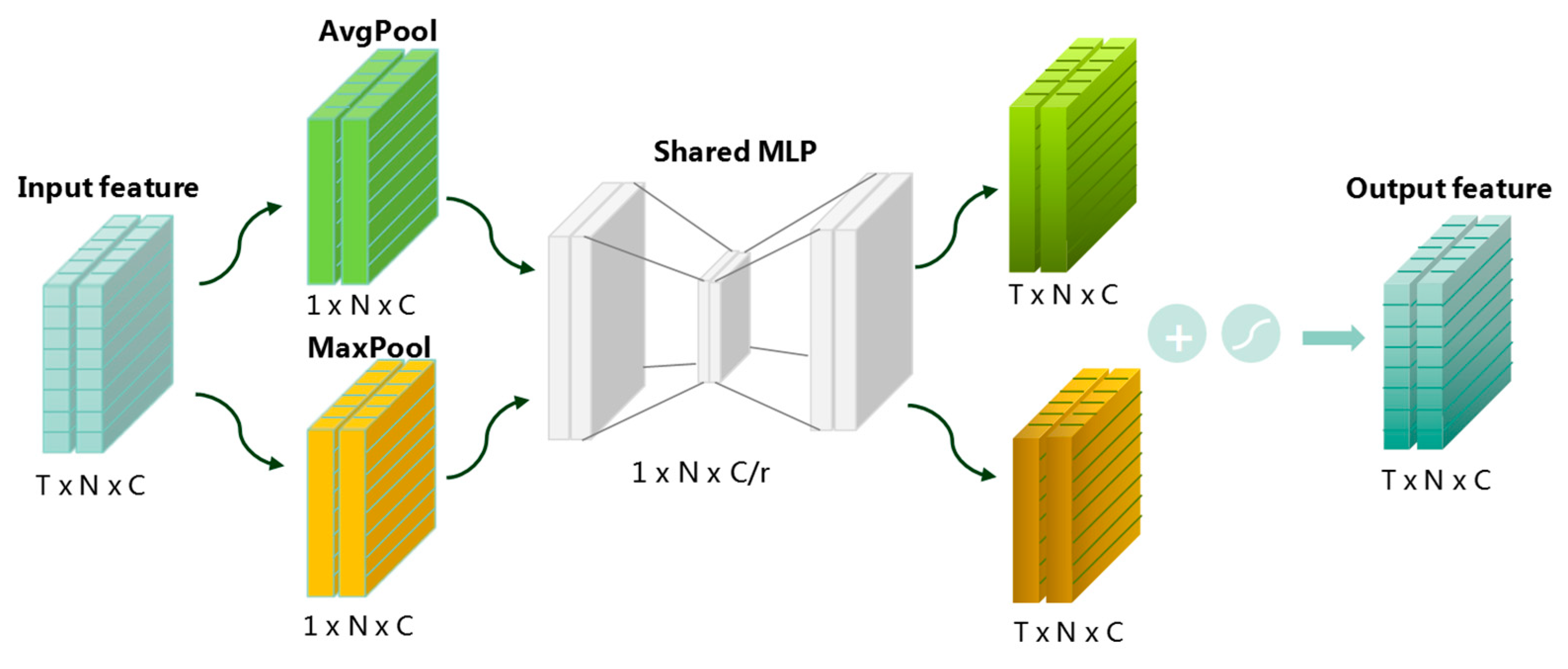
When predicting the next period based on the existing observation information, if the same weight is given to the pedestrian trajectory coordinates, it will cause insufficient attention to one coordinate direction, and excessive attention to the other coordinate direction. Then, it cannot effectively explore the motion characteristics of pedestrians in different orientations. Similarly, for each moment in the observation time $t_o\in \left\{1,2,\dots ,o\right\}$, each moment has a different degree of influence and importance for the subsequent trajectory prediction; for example, when a pedestrian makes an unconventional movement such as a turn or a stop, the importance of the input for prediction varies from one observation moment to another. Therefore, the weighting module of temporal information (TIW) proposed in this paper is no longer in the previous form, but fully extracts the information of pedestrian trajectory coordinates $v_t^j$ and each moment in the observed time $t_o$, fuses them separately, and assigns different weights to the historical trajectory information of the pedestrian.

The temporal information weighting module first integrates the pedestrian trajectory data into a matrix ${F\in {ℝ}^{} }^{T\times N\times C}$ as the input to the module.

As shown in Figure 1, N is the number of pedestrians, T is the total length of the observation time, and C includes information on the x and y coordinates of the pedestrians. Then, the pedestrian trajectory information is input into the convolutional network to operate on the pedestrian historical time-series trajectory; the trajectory information between the observation periods is given different weights by convolution, and then, superimposed with the pedestrian trajectory information to obtain the pedestrian trajectory information after module processing. The structure of the temporal information weighting module is as follows.

The model in this paper obtains the output by fusing the weighted information of the location $v_t^i=\left(x_t^i,y_t^i\right)$ of the i-th pedestrian at each moment $t\left(t\in t_o\right)$ in the period $t_o$.

The first step of the weighted fusion of temporal information is to extract temporal features from the trajectory information of the i-th pedestrian in period $t_o$, assign different weights to the position information x and y at each moment $t$, and then, sum up with the corresponding original coordinate information in the corresponding moment to obtain the output result $M_T^i\left(F\right)$, as shown in (4):

$$\begin{array}{c}{M}_T^i\left(F\right)=\sigma \left(MLP\left(AvgPool\left(F\right)\right)+MLP\left(MaxPool\left(F\right)\right)\right)\\ =\sigma \left(W_{T1}\left(W_{T0}\left(F_{avg}^T\right)\right)+W_{T1}\left(W_{T0}\left(F_{\max }^T\right)\right)\right)\end{array}$$

(4)

where σ denotes the sigmoid function, $W_{T0}\in {ℝ}^{C/r\times C}$, and $W_{T1}\in {ℝ}^{C\times C/r}$. The shared network consists of a multi-layer perceptron (MLP) whose weights $W_{T0}$ and $W_{T1}$ are shared, and the ReLU activation function, followed by $W_{T0}$.

2.3. Spatial Interaction Module of Multi-Pedestrians

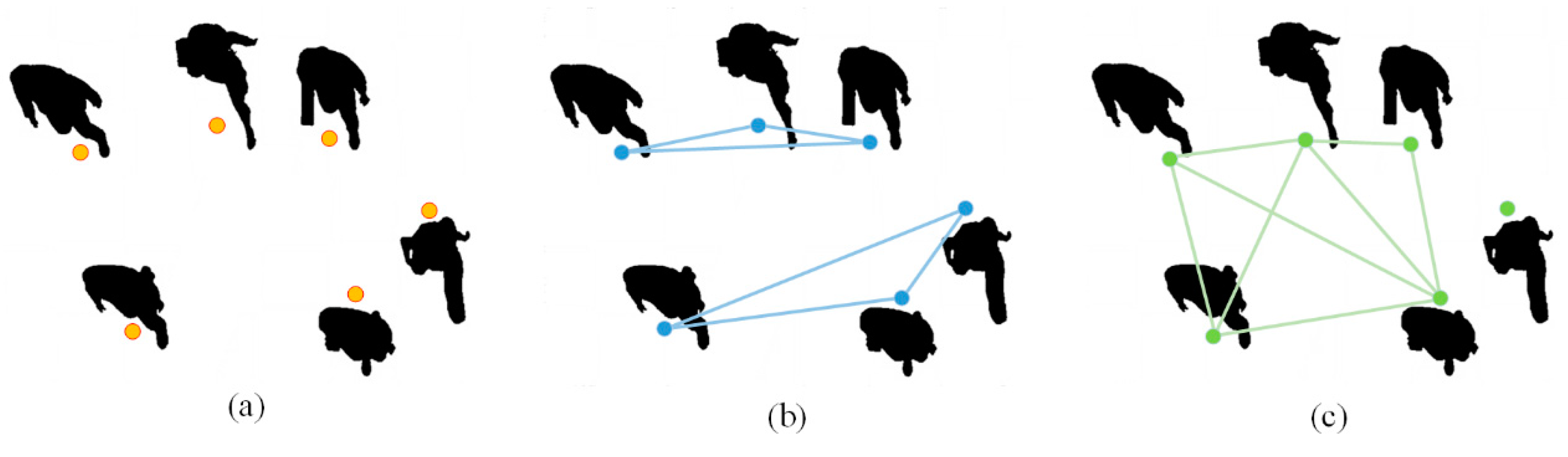
Although it is quite advanced to integrate the spatial interaction information of pedestrians into existing models, integrating spatial interaction information among all pedestrians at one time will lead to redundant information. This paper addresses this problem by proposing a spatial interaction module for multi-pedestrians. The statistical analysis of pedestrian aggregation and the number of mainstream clusters is performed through the ETH [29] and UCY [30] datasets, and this paper combines the analysis results to classify the pedestrian spatial interaction into three types of aggregate according to the number of pedestrians, as shown in Figure 2. In the first category (a), each pedestrian is considered independently as an aggregate, and the influence between the aggregates is considered; in the second category (b), three people are considered as an aggregate and only the interaction between these three people is considered as a case of small-scale aggregated interaction; in the third category (c), five people are considered as an aggregate, and only the interaction between these five pedestrians is considered as a case of large-scale aggregated interaction. The reason we chose the three types of aggregate above is explained in detail in the ablation test in the Ablation Experiments part of Section 3. At the same time, this paper uses a convolution calculation formula (5) to set the number of pedestrians in the aggregate (1, 3, and 5).

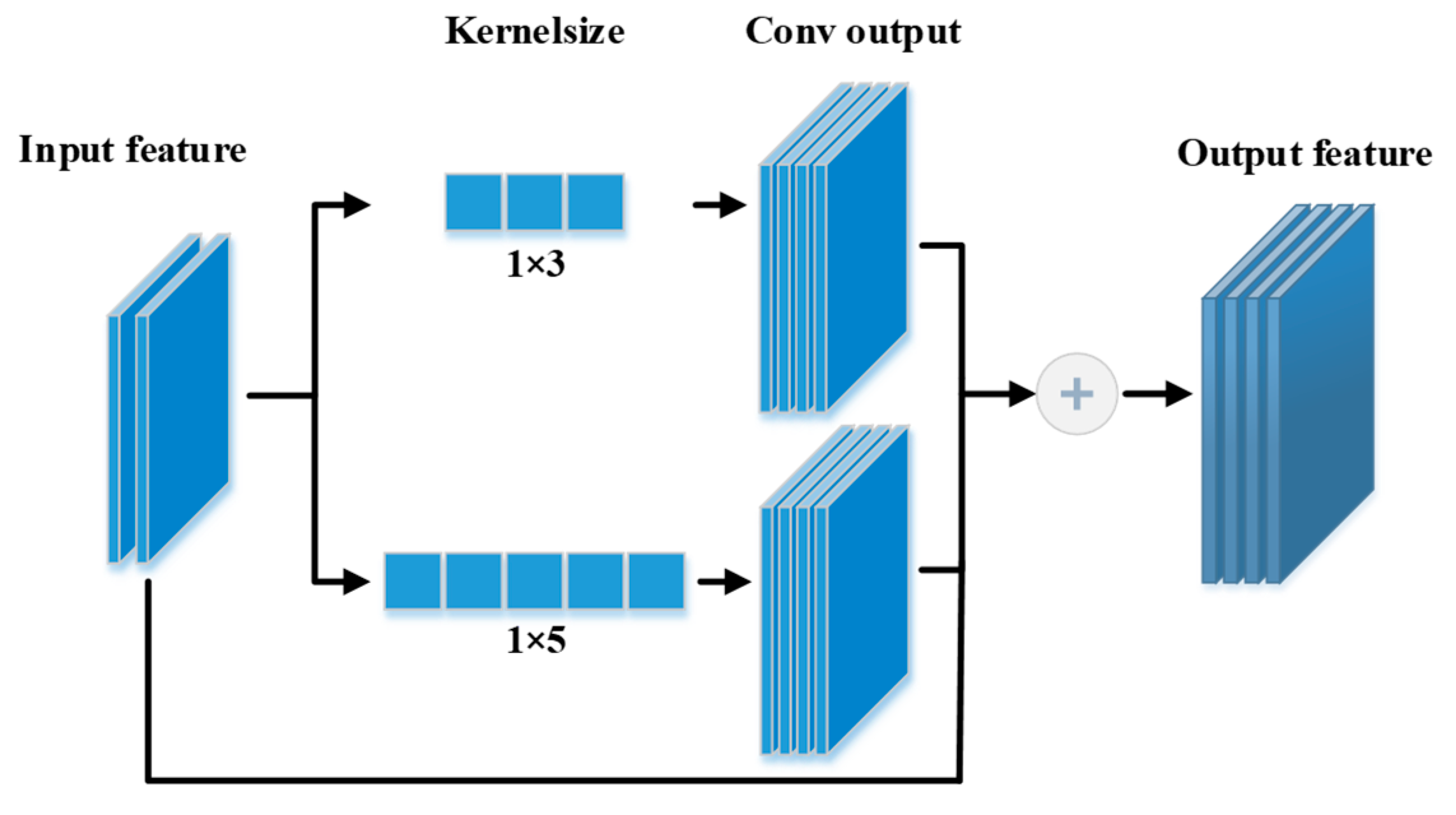
With the spatial interaction module of multi-pedestrians (M-PSI), the model in this paper can effectively obtain interaction information between pedestrians in multiple aggregation situations. By superimposing the interaction information between pedestrians in multiple different modes, the impact of redundant interaction information generated by the network on future trajectory prediction is reduced. The aim of the implementation of the method in this thesis is to obtain the same dimensional information by convolving the pedestrian feature information in different ways, and then, superimposing the information with the input pedestrian features. The structure uses multiple convolutional kernels of different sizes to achieve the extraction of interaction information between pedestrians in the convolution. According to the convolution formula, the output in the pedestrian number dimension is shown in (5):

$$Nums=\frac{Num-\mathrm{kernelsize}+2\times \mathrm{padding}}{\mathrm{stride}}+1$$

(5)

Num represents the number of pedestrians, kernel size represents the size of the convolution kernel in the pedestrian number dimension, padding represents padding, stride represents the step size, and Nums represents the output after convolution.

As shown in Figure 3, the spatial interaction module of multi-pedestrians in this paper is a three-level module with a two-dimensional convolution. To ensure that no redundant time-dimensional interactions are generated, the sizes of the convolution kernels are set to 1 × 3 and 1 × 5, respectively, and the original input information is superimposed and fused with the convolution output to obtain the output information.

Additionally, by filling the number of pedestrians dimensionally, the convolution is carried out properly and the consistency of the convolution output is guaranteed. This ensures that the spatial interaction information of pedestrians at the corresponding moment is extracted efficiently, and no temporal interaction is generated, which is implemented in (6).

$$\begin{array}{c}{m}_0=M_T^i\left(F\right)\\ m_1=CONV\left(M_T^{i-1}\left(F\right),M_T^i\left(F\right),M_T^{i+1}\left(F\right),W_1\right)\\ m_2=CONV\left(M_T^{i-2}\left(F\right),M_T^{i-1}\left(F\right),M_T^i\left(F\right),M_T^{i+1}\left(F\right),M_T^{i+2}\left(F\right),W_2\right)\\ o_i=m_0+m_1+m_2\end{array}$$

(6)

where $W_1$ is the parameter of 1 × 3 convolution, $W_2$ is the parameter of 1 × 5 convolution, $m_0$ is the output of single-person interaction, $m_1$ is the output of three-person interaction, and $m_2$ is the output of five-person interaction. $o_i$ is the output of multimodal i-th pedestrian space interaction.

2.4. View-Direction Graph

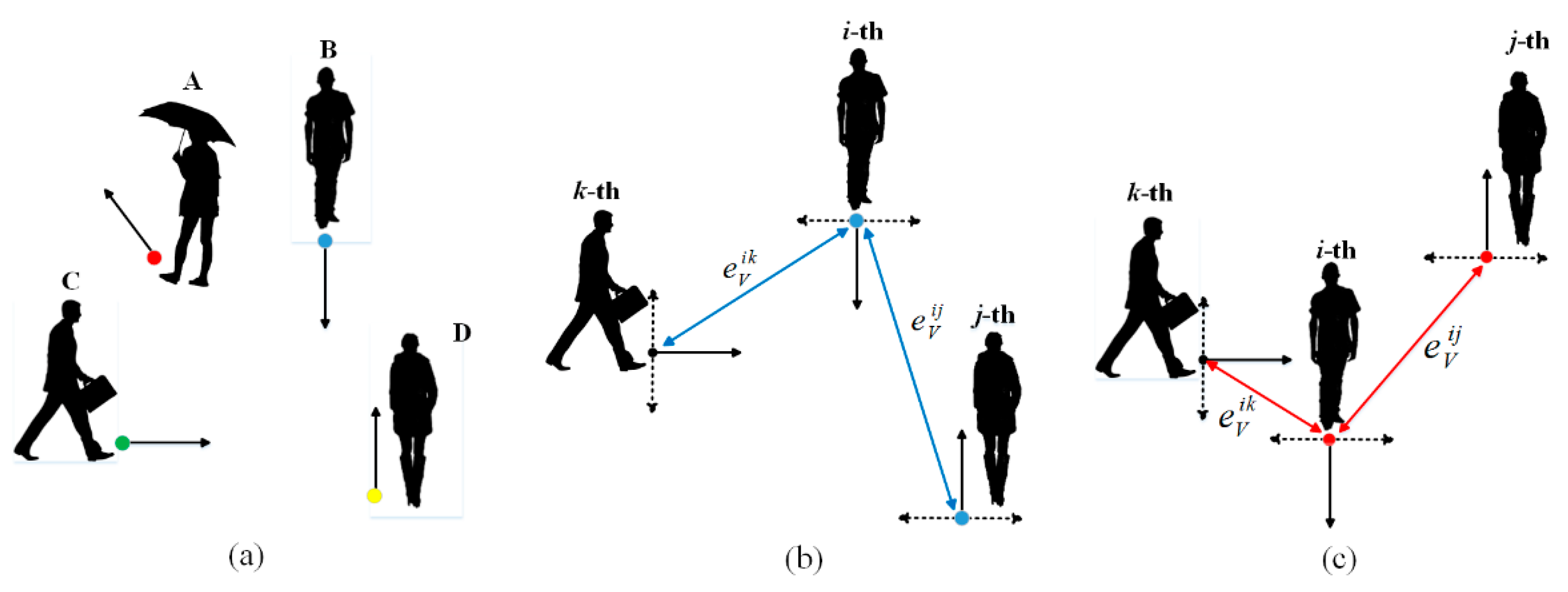
Intuitively, a pedestrian’s movement behavior is significantly influenced by other pedestrians in his or her field of view. For example, while walking, we are always aware of pedestrians within our field of view. As shown in Figure 4a, pedestrian A cannot see any pedestrians, so her motion is not influenced by other pedestrians. However, since she appears in the field of view of pedestrians B, C, and D, her behavior may affect their future movements. Inspired by this situation, we construct a View Graph (VG) of the pedestrian’s field of view based on the horizontal view of the pedestrian. In the model, we assume that the pedestrian moves forward along the observation trajectory and that the pedestrian’s field of view is set to be a sector with a tensor angle of π. The parallels of the pedestrian’s field of view coincide with his/her direction of motion. For simplicity, we set the field of view of the pedestrian to π, which we can see in Figure 4b.

The View Graph is defined as $G_V=\left(V,E_V\right)$. If the j-th pedestrian is in the view of the i-th pedestrian, $e_V^{ij}$= 1 if $v_t^i$ and $v_t^j$ are connected; otherwise, $e_V^{ij}$= 0, in which $a_t^{ij}$ is weighted by the kernel function and defined as follows.

$$e_V^{ij}=\{\begin{array}{ll}\frac{1}{{\Vert v_t^i-v_t^j\Vert }_2}& , \left[\Delta v_t^i\left(v_t^i-v_t^j\right)\right]\left[\Delta v_t^j\left(v_t^i-v_t^j\right)\right]>0\\ 0& , \mathrm{otherwise} \end{array}$$

(7)

where $\Delta v_t^i=v_{t+1}^i-v_t^i$ indicates the direction of motion of the i-th pedestrian. We illustrate the topology of the VG further in Figure 4. Figure 4b shows that since the angle between the i-th pedestrian and the j-th pedestrian is smaller than π/2, they influence each other, so $e_V^{ij}$ is not 0; however, if the angle between the i-th pedestrian and the j-th pedestrian is greater than π/2 in Figure 4c, they have entered blind spots in each other’s vision; thus, $e_V^{ij}$= 0.

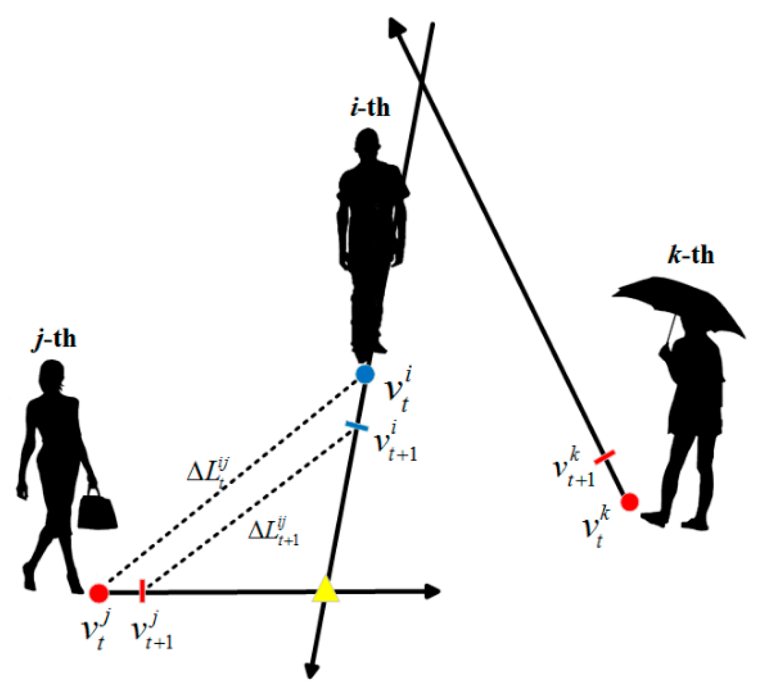
The VG presented in the previous section utilizes only the location information of pedestrians. In crowded situations, we also need to be aware of pedestrians who may be in potential conflict. In this section, we propose a Direction Graph (DG) $G_D=\left(V,E_D\right)$, where $E_D=\left\{e_D^{ij}|\forall i,j\in \left\{1,\dots ,N\right\}\right\}$, and the impact of conflicts between pedestrians is described by determining the direction of their movement. If the movement directions of two pedestrians intersect, we can assume that they have a potential collision risk. Figure 5 shows that the possibility of collision exists between the i-th and j-th pedestrians. The impact between them satisfies the following constraint.

$$e_D^{ij}=\{\begin{array}{ll}\frac{1}{{\Vert v_t^i-v_t^j\Vert }_2}& , \Delta L_t^{ij}>\Delta L_{t+1}^{ij}\\ 0& , \mathrm{otherwise} \end{array}$$

(8)

where $\Delta L_t^{ij}$ represents the spatial distance between the i-th pedestrian and j-th pedestrian at time t, i.e., $\Delta L_t^{ij}=v_t^i-v_t^j$.

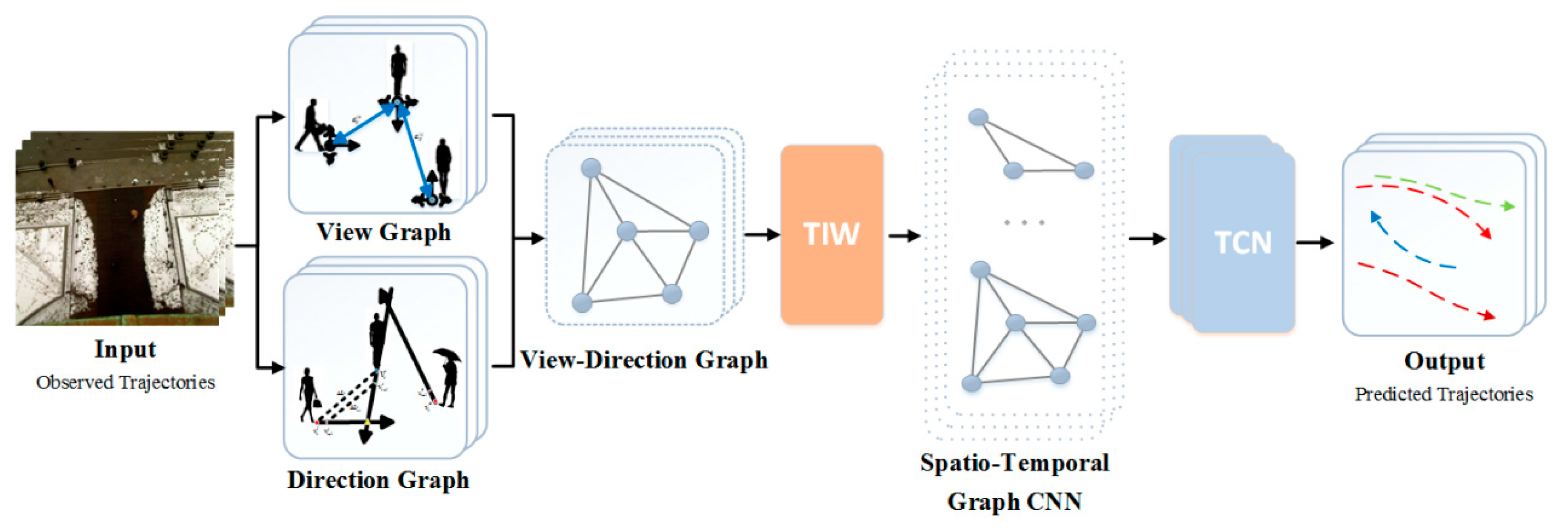
2.5. View-Direction Graph Convolutional Neural Network

In this subsection, we propose a View-Direction graph (V-DG) convolutional neural network framework for trajectory prediction. The framework of our proposed method is shown in Figure 6, and consists of three main components, i.e., topological graph fusion, graph convolution, and temporal convolution. We use a multilayer perceptron (MLP) to fuse the pedestrian interaction information in VG and DG to form a unified topological graph structure. If we assume that there are N pedestrians in the scene at time t, we can construct weighted adjacency matrices of all edges in VG and DG according to (6) and (7), respectively. Then, we stack them onto a tensor of $N\times N\times 2$ and use MLP to adaptively fuse the weighted edges. Finally, we obtain the weighted adjacency matrix $E_{V-D}\in {ℝ}^{N\times N\times 1}$, which fuses the features of VG and DG. The matrix fusion process is performed as follows:

$$E_{V-D}=MLP\left(E_V,E_D\right)$$

(9)

where the input size of the graph fusion module is $N\times N\times 2o$ and the output size is $N\times N\times o$.

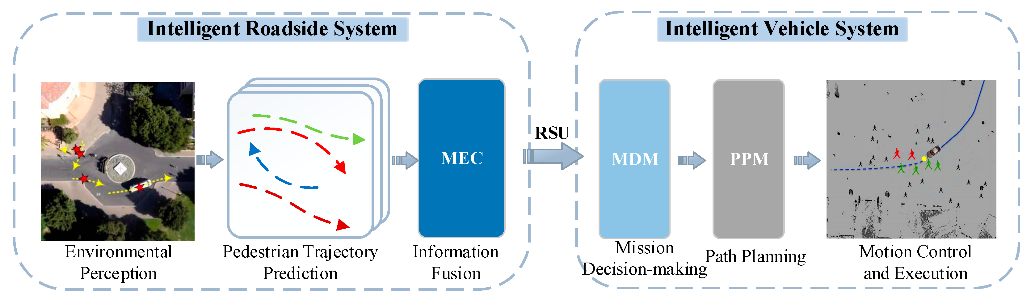
2.6. Autonomous Driving Obstacle Avoidance System

To better apply the pedestrian trajectory prediction model proposed in this paper, in this section, we design an autonomous driving obstacle avoidance system based on pedestrian trajectory prediction, which is shown in Figure 7. The system consists of two parts: the intelligent roadside system and the intelligent vehicle system. Firstly, the intelligent roadside system performs image acquisition through the roadside camera for pedestrian trajectory prediction and sends the information to multi-access edge computing (MEC) for information fusion; then, it transmits the processed roadside data to the intelligent vehicle system through the roadside unit (RSU). The system performs subsequent mission decision-making, path planning, and motion control execution. With the above two subsystems, we can achieve active obstacle avoidance for autonomous driving. Meanwhile, because our proposed pedestrian trajectory prediction model has a fast inference speed, which we will introduce in detail later, this autonomous driving obstacle avoidance system can achieve faster responses in real-time to road emergencies.

3. Experiments

3.1. Datasets and Evaluation metrics

The model we propose is trained on two pedestrian trajectory prediction datasets: the ETH and the UCY. The ETH contains two scenarios (ETH and HOTEL), and the UCY contains three scenarios (ZARA1, ZARA2, and UNIV). These datasets contain the real motion trajectories of a total of 1536 pedestrians, implying a wide variety of pedestrian interactions and challenging social behaviors. In the experiments on the datasets, this paper uses four datasets to train the model, and then, tests it on the remaining one dataset. In the evaluation phase, the model predicts the later 4.8 s pedestrian trajectories by observing the first 3.2 s pedestrian trajectories.

Following our previous work, we compare this model with existing models, and, as with existing methods, we use two error metrics to evaluate and express the performance of the proposed method.

Average displacement error (ADE): This is obtained by calculating the average Euclidean distance between the predicted trajectory and the true trajectory for each pedestrian in all prediction time steps, and a smaller value indicates a better prediction. ADE is defined as follows.

$$ADE=\frac{{\displaystyle {\sum }_{i=1}^N{\displaystyle {\sum }_{t=o+1}^{o+p}{\Vert {{\displaystyle \widehat{v}}}_t^i-{{\displaystyle v}}_t^i\Vert }_2}}}{N\times p}$$

(10)

Final Displacement Error (FDE): This is obtained by calculating the average Euclidean distance between the predicted trajectory and the true trajectory for each pedestrian’s position in the final prediction time step, and a smaller value indicates a better prediction. FDE is defined as follows.

$$FDE=\frac{{\displaystyle {\sum }_{i=1}^N{\Vert {{\displaystyle \widehat{v}}}_{o+p}^i-{{\displaystyle v}}_{o+p}^i\Vert }_2}}{N}$$

(11)

We compare our proposed model with eleven recently proposed models in terms of both ADE and FDE, mainly including the following: Social-LSTM [9]: A neural network-based algorithm for pedestrian trajectory prediction that uses an LSTM model and a social pool model to learn the sequence characteristics and social behavior of pedestrians, respectively; Social-GAN [7]: a GAN-based method for multimodal pedestrian trajectory generation; PIF [31]: a multi-task LSTM model using visual features and interactive features; SoPhie [11]: a model that employs an attentional GAN to consider physical constraints and social concerns; SR-LSTM [13]: a state refinement method for extracting the social features of pedestrian trajectories; STSGN [32]: an LSTM approach for the graph-attention-based modeling of pedestrian social interactions; CGNS [33]: a conditional generation network based on the GRU model; Social-BiGAT [34]: a bicycle-GAN multimodal path and pedestrian social interaction model with a GAT module; TPNSTA [24]: a pedestrian pyramid network trajectory prediction model with spatio-temporal attention; Social-STGCNN [21]: a social spatio-temporal graph convolutional neural network for human trajectory prediction; and Trajectron++ [35]: a CVAE-based model that incorporates agent dynamics and semantic maps.

3.2. Model Construction and Training Setup

The model in this paper includes a V-DG information fusion module, a temporal information weighting module, a spatial interaction module of multi-pedestrians, and a temporal convolutional network module consisting of four TCN layers. Experiments on the number of module stacks verify that a spatial interaction module of multi-pedestrians and a stack of four TCN layers work best for pedestrian trajectory prediction. The training batch size is set to 128. The activation function used for the model in this paper is PReLU, and stochastic gradient descent (SGD) is used to train the model 250 times. The initial learning rate is 0.01, and the learning efficiency changes to 0.002 after another 150 times. The experiments in this paper are conducted under the same hardware conditions; the experimental computer uses an Intel Core i7-10875k CPU @2.3 GHz with 8 cores and 16 threads, and the graphics card is an NVIDIA 2060 Max-Q GPU with 6 GB video memory.

3.3. Quantitative Analysis

Model comparison: In this subsection, we compare the model we propose, At-VD-GCN, with the eight methods that have been mentioned above.

Table 1. ADE/FDE metrics for several methods compared to At-VD-GCN are shown. The models marked with * are non-probabilistic. The rest of models use the best amongst 20 samples for evaluation. All models take 8 frames as an input and predict the next 12 frames. We notice that At-VD-GCN has the best average error on both ADE and FDE metrics (the lower the better).

Stochastic	ETH	Hotel	Univ	Zara1	Zara2	AVG
S-LSTM	1.09/2.35	0.79/1.76	0.67/1.40	0.47/1.00	0.56/1.17	0.72/1.54
S-GAN	0.81/1.52	0.72/1.61	0.60/1.26	0.34/0.69	0.42/0.84	0.58/1.18
SoPhie	0.70/1.43	0.76/1.67	0.54/1.24	0.30/0.63	0.38/0.78	0.54/1.15
Social-BiGAT	0.69/1.29	0.49/1.01	0.55/1.32	0.30/0.62	0.36/0.75	0.48/1.00
SR-LSTM *	0.63/1.25	0.37/0.74	0.51/1.10	0.41/0.90	0.32/0.70	0.45/0.94
STGAN	0.65/1.12	0.35/0.66	0.52/1.10	0.34/0.69	0.29/0.60	0.43/0.83
TPNSTA	0.55/0.91	0.23/0.40	0.52/1.10	0.34/0.70	0.26/0.55	0.38/0.73
Social-STGCNN	0.64/1.11	0.49/0.85	0.44/0.79	0.34/0.53	0.30/0.48	0.44/0.75
STAR	0.36/0.65	0.17/0.36	0.31/0.62	0.26/0.55	0.22/0.46	0.26/0.53
SGCN	0.63/1.03	0.32/0.55	0.37/0.70	0.29/0.53	0.25/0.45	0.37/0.65
Trajectron++ *	0.71/1.68	0.22/0.46	0.41/1.07	0.30/0.77	0.23/0.59	0.37/0.91
Ours	0.44/0.76	0.14/0.23	0.26/0.50	0.22/0.44	0.15/0.32	0.26/0.46

shows the experimental results obtained for each model in five scenarios included in the two datasets, and the average results for each pedestrian trajectory prediction method are given in the last column, with the red values in the table representing the best results and the blue values representing the second best results. Based on the experimental results, we can analyze and draw the following conclusions.

We can visually see that our proposed model achieves the best or second-best results for each scenario of the test datasets. Furthermore, our proposed method, At-VD-GCN, achieves the best performance on both the average ADE and FDE results, resulting in a prediction performance improvement of at least 6%/16% or more.

Compared with the base model, Social-STGCNN, our algorithm outperforms Social-STGCNN on all datasets, improving the prediction performance by about 32% and 38% on the average ADE and FDE results, respectively. This validates that the information fusion graph convolutional network we propose describing pedestrian interactions indeed helps to improve social interactions and make them more relevant and accurate.

When no scene information is in consideration, our method, At-VD-GCN, still predicts better than those methods that utilize scene features, such as [11,31,34]. This suggests that the prediction performance of At-VD-GCN can be further improved by incorporating the background information of the scene in which the pedestrian is located.

3.3.1. Inference Speed and Model Size

The size of the model we propose is 6.16 K parameters, which is less than that of the Social-STGCNN. A comparison of the model parameters and inference time between our model and the models available for public use is shown in the following table, where the inference time is the average of some single inference steps, and the lower the inference time, the better. The reason for these results in this model is that the model uses only convolutional neural networks, which overcomes the two major limitations of recursive architecture and the aggregation mechanism.

Table 2. A comparison table of each model’s parameters and inference speed.

Stochastic	Parameters Count	Inference Time(s)
S-LSTM	264 K	1.1789
SR-LSTM-2	64.9 K	0.1578
S-GAN-P	46.3 K	0.0968
PIF	360.3 K	0.1145
Social-STGCNN	7.6 K	0.0020
Ours	6.16 K	0.0014

shows a comparison table of each model parameter and inference speeds, where our model inference times are the results of tests using the edge device NVIDIA Jetson TX2.

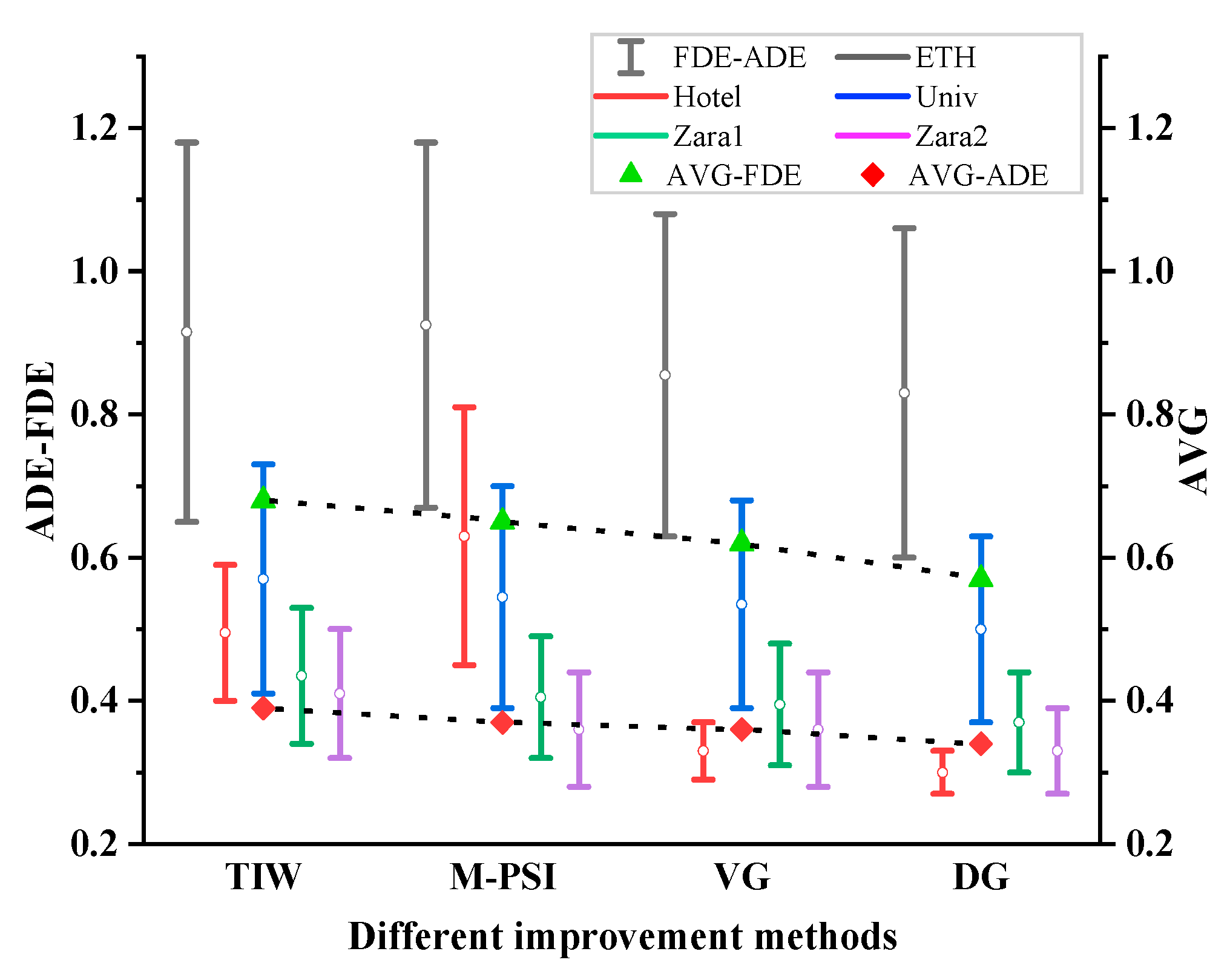
3.3.2. Ablation Experiments

To further analyze the impacts of different improvement methods on the performance of the Social-STGCNN algorithm, four sets of experiments are designed to analyze the different improvement methods. In these experiments, ADE and FDE are used as evaluation metrics for the experiments, as shown in

Table 3. The results of ADE/FDE obtained through ablation experiments.

TIW	M-PSI	VG	DG	ETH	Hotel	Univ	Zara1	Zara2	AVG
√	×	×	×	0.65/1.18	0.40/0.59	0.41/0.73	0.34/0.53	0.32/0.50	0.39/0.68
√	√	×	×	0.67/1.18	0.45/0.81	0.39/0.70	0.32/0.49	0.28/0.44	0.37/0.65
√	√	√	×	0.60/1.06	0.27/0.33	0.37/0.63	0.30/0.44	0.27/0.39	0.34/0.57
√	√	√	√	0.44/0.76	0.14/0.23	0.26/0.50	0.22/0.44	0.15/0.28	0.26/0.46

, where “√” indicates that the improvement method is introduced in the model and “×” indicates that the method is not introduced in the model. The effects of different improvement methods on the datasets for ETH and UCY are shown in Figure 8, and it can be seen that all the improvement methods proposed in this paper can improve the prediction accuracy to some extent.

To ensure that the spatial interaction module of multi-pedestrians (M-PSI) that we propose can express the influence between multiple individuals, we focus on the distribution of pedestrian groups in the ETH and UCY datasets. An ablation experiment, which includes a total number of pedestrians from 1 to 7, is carried out. As shown in

Table 4. The results of different pedestrian numbers obtained through ablation experiments.

Number of Pedestrians	1	2	3	4	5	6	7
ETH	0.67/1.18	0.77/1.27	0.65/1.17	0.74/1.27	0.66/1.19	0.80/1.25	0.72/1.23
Hotel	0.45/0.81	0.53/0.90	0.43/0.82	0.52/0.87	0.47/0.78	0.55/0.94	0.49/0.88
Univ	0.39/0.70	0.46/0.81	0.40/0.72	0.49/0.81	0.41/0.70	0.50/0.80	0.47/0.79
Zara1	0.32/0.49	0.40/0.58	0.30/0.48	0.45/0.59	0.35/0.49	0.47/0.60	0.40/0.58
Zara2	0.28/0.44	0.36/0.55	0.25/0.45	0.35/0.53	0.30/0.45	0.38/0.55	0.34/0.50
AVG	0.37/0.65	0.47/0.75	0.36/0.63	0.46/0.79	0.37/0.63	0.49/0.80	0.43/0.71

, it can be seen that the number of pedestrians is set to 1, 3, and 5, and the results of trajectory prediction are superior to those of the other cases. Therefore, to optimize the interaction effect between pedestrians, we designed the M-PSI module to analyze the weighted fusion of the three scenarios to obtain more accurate pedestrian interaction information.

3.4. Qualitative Analysis

In the quantitative analysis section, it is shown that the model proposed in this paper outperforms the previous level in ADE/FDE metrics. Now, we qualitatively analyze why the temporal information weighting module of this paper’s model improves the effectiveness of trajectory information; how the spatial interaction module of pedestrian assemblies can better achieve the information extraction of pedestrian aggregation situations; and how the View-Direction graph information fusion module reduces redundant information and describes the pedestrian interaction situation more accurately.

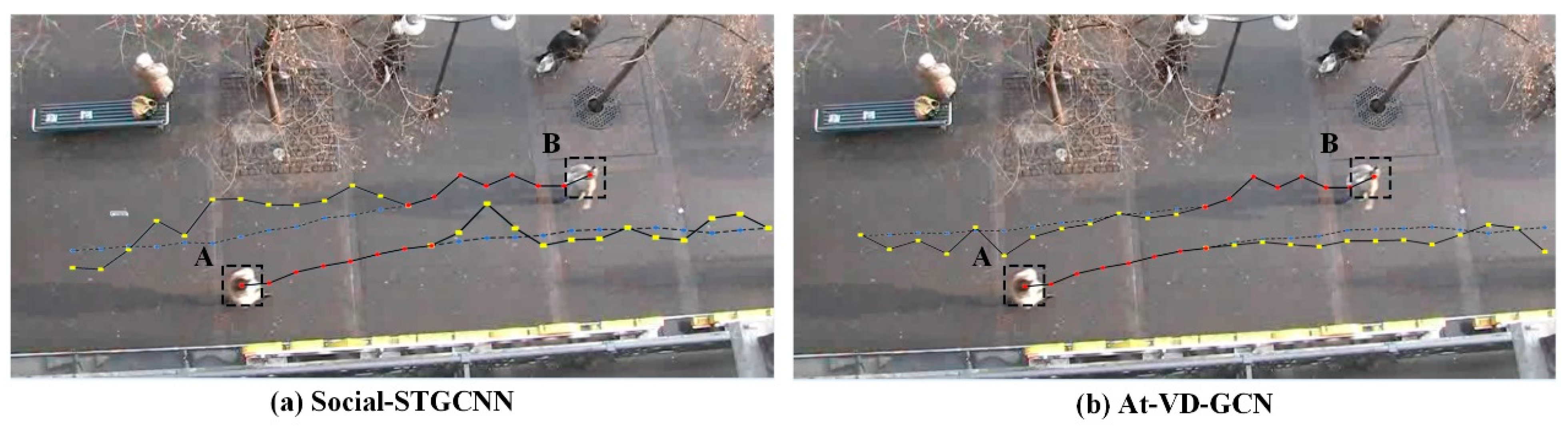
When pedestrians walk, they may turn left or right, accelerate or decelerate, and stop due to various road conditions, in addition to walking straight in a certain direction. Simply giving the same weight to the information at each observation moment will affect the validity of the information. In this paper, the temporal information weighting module gives different weights to the trajectory information of the pedestrian observation phase at each moment, so that the model can focus on the coordinate information of an important moment. As shown in the trajectory comparison in Figure 9, the model in this paper gives more weight to the coordinate information of the important moments of the trajectory by considering the historical trajectory information of the observation phase, and the predicted pedestrian trajectory is more consistent with the real trajectory.

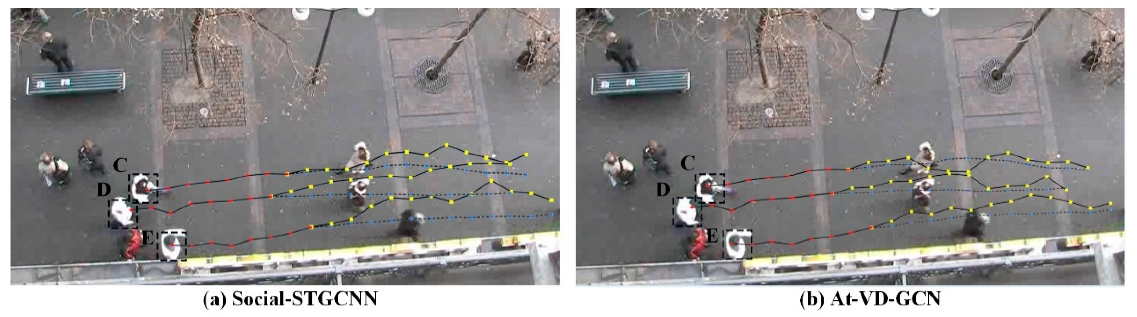
When groups of two or more people walk together, they are usually spatially close to each other and have similar movement speeds and walking directions, which are defined as pedestrian aggregates in the spatial interaction module of multi-pedestrians. In Figure 10, the walking routes of pedestrians C, D, and E are parallel to each other. From Figure 10a, it can be seen that although the predicted trajectory results obtained based on Social-STGCNN can maintain the tightness of the group, there is great deviation from the real trajectory on the ground. In contrast, the prediction results of our model, At-VD-GCN, in Figure 10b show that C, D, and E as an aggregate of pedestrians will keep walking parallel to each other, and the predicted trajectories have much less deviation from the ground truth trajectories. This is because the model in this paper fully considers the interaction and influence of pedestrians within different pedestrian aggregates, which reduces the influence of redundant information when interacting in large-scale pedestrian scenarios and makes the predicted pedestrian trajectories more accurate.

4. Conclusions

In this paper, we showed that a graph-based spatio-temporal setup for pedestrian trajectory prediction improves previous methods in several key aspects, including prediction error, computational time, and number of parameters. By applying the View-Direction graph to describe the social interaction between pedestrians and weighting the pedestrian trajectory with temporal information, At-VD-GCN outperforms state-of-the-art models when applied to a number of publicly available datasets. We also qualitatively analyzed the performance of At-VD-GCN under situations such as collision avoidance, parallel walking, and individuals meeting in groups. In these situations, At-VD-GCN tends to provide more realistic path forecasts than several other reported methods. Furthermore, At-VD-GCN is also efficient computationally, and its inference speed is increased compared to previous models. In the future, we intend to extend At-VD-GCN to multi-modal settings that involve other moving objects, including bicycles, cars, and pedestrians.