Spatio-Temporal Transformer Recommender: Next Location Recommendation with Attention Mechanism by Mining the Spatio-Temporal Relationship between Visited Locations

Abstract

Location-based social networks (LBSN) allow users to socialize with friends by sharing their daily life experiences online. In particular, a large amount of check-ins data generated by LBSNs capture the visit locations of users and open a new line of research of spatio-temporal big data, i.e., the next point-of-interest (POI) recommendation. At present, while some advanced methods have been proposed for POI recommendation, existing work only leverages the temporal information of two consecutive LBSN check-ins. Specifically, these methods only focus on adjacent visit sequences but ignore non-contiguous visits, while these visits can be important in understanding the spatio-temporal correlation within the trajectory. In order to fully mine this non-contiguous visit information, we propose a multi-layer Spatio-Temporal deep learning attention model for POI recommendation, Spatio-Temporal Transformer Recommender (STTF-Recommender). To incorporate the spatio-temporal patterns, we encode the information in the user’s trajectory as latent representations into their embeddings before feeding them. To mine the spatio-temporal relationship between any two visited locations, we utilize the Transformer aggregation layer. To match the most plausible candidates from all locations, we develop on an attention matcher based on the attention mechanism. The STTF-Recommender was evaluated with two real-world datasets, and the findings showed that STTF improves at least 13.75% in the mean value of the Recall index at different scales compared with the state-of-the-art models.

1. Introduction

With the development of information communication and mobile technologies, location-based Social Networks (LBSNs) become increasingly popular in people’s daily life. LBSNs provide users with unique ways to share their data, providing new data sources for data mining and machine learning. Specifically, these data include users’ locations, views, photos, and comments, and spatio-temporal big data gathered from these platforms have been widely used in different applications, such as the study of individual activity patterns [1], next point-of-interest (POI) recommendation [2], etc. In particular, users’ check-ins are captured as a set of visit locations (i.e., trajectories) by the LBSNs when users go to a certain POI. On the one hand, these check-ins contain rich information about users’ daily movement by recording visited POIs, as well as specific visiting times and visit frequency of a POI for each user. By analyzing a user’s historical trajectories, we can roughly understand the user’s movement patterns and living habits. On the other hand, multiple users’ check-in frequency and check-in time of a certain POI can provide more accurate information to describe the temporal visit patterns of the users. By analyzing the historical trajectories of all users in LBSNs, such POI information and their inherent spatio-temporal relationship can be mined by incorporating machine learning algorithms, such as deep learning methods [3].

Recent work in POI recommendation with LBSNs data primarily focuses on identifying where specific users went and when. This information is of great significance for individual travel planning, business site selection, and urban planning [4]. Individual users, even in unfamiliar cities, can find places suitable for their interests and hobbies, which facilitates and enriches people’s lives. For businesses, the POI recommendation research can help understand customer needs and therefore plan more targeted advertisements for specific user groups, which can significantly improve the efficiency of advertising and save publicity costs while gaining customer visits more effectively and achieving revenue growth. For the government, this research can enable urban planners to understand the users’ movement patterns of the whole city from an overall perspective, which can help improve urban transportation, plan urban road networks, and monitor abnormal movement behaviors of citizens and traffic more timely. As a result of these societal benefits, much effort and progress have been made in POI recommendation research [5]. Specifically, early research mostly focused on non-deep learning-based methods, requiring handcrafted feature engineering [6], and cannot properly utilize the spatio-temporal information contained in LBSNs. With the recent advancement of machine learning techniques, a large number of deep learning-based POI recommendation models, such as Recurrent Neural Network (RNN) and Convolutional Neural Network (CNN), have been developed.

However, most of the current research only focuses on adjacent POI visits and ignores non-contiguous visits. In fact, these non-contiguous visits are very helpful in understanding users’ movement behavior and capturing long-term preferences of user trajectory sequence. In particular, the spatio-temporal relationship between LBSNs can be explored from two aspects: spatio-temporal aggregation and long-term preferences of user trajectory sequence. Spatio-temporal aggregation refers to aggregating relevant visited locations from spatio-temporal relationships between user visits. The long-term preferences denote a user’s general interests mined from her/his historical trajectories, which are usually stable. Unfortunately, most deep learning-based approaches for modeling user preferences are unable to model the relations between two nonconsecutive POIs, as they can only model consecutive activities in the user’s check-in sequence. Moreover, many existing models fail to fully leverage spatial and temporal patterns of POI visits while mining these temporal and spatial data. For example, Sun et al. [7] proposed a geo-dilated RNN model to aggregate the most recently visited locations, but only for spatial preferences. In terms of spatial patterns, POI recommendations need to consider the distance between two locations, which may not appear sequentially in previous users’ POI visit sequences but may be visited together due to their proximity. In terms of temporal patterns, different from shopping behavior patterns with having a likely non-continuous sequence, POI visits often present aggregation in time. Examples of trajectories with the relation between non-consecutive visits and non-adjacent locations are shown in Figure 1. Examples of trajectories showing the relation between non-consecutive visits and non-adjacent locations. The map shows the spatial distribution of visited locations, which are numbered from 1 to 5. Solid marks 1, 2, and 3 indicate the user’s usual weekday check-ins, and hollow marks 4 and 5 indicate weekend check-ins. These visits show correlations between non-adjacent locations and non-contiguous visits, which are spatially distant and temporally regular. However, many existing models only recommend locations that are adjacency to previously visited POIs, which may impact the results. In order to learn the spatio-temporal relationship between users’ visits, we encode the information in the user’s trajectory as latent representations into their embeddings before feeding them into other modules. This embedding method can better reflect users’ spatial preferences and discover temporal periodicity.

Much of the previous work only used explicit spatio-temporal intervals between two successive visits in a recurrent layer and ignored discontinuous visits, which would prevent the model from learning the long-term preference of the user trajectory sequence [8]. STRNN [9], for example, applies the spatio-temporal interval directly between successive visits in an RNN. DeepMove [10] combines the attention layer with the recurrent layer to learn the multi-level periodicity of sequences from relevant trajectories, respectively. However, none of these models can directly capture the dependencies between any two visits. In order to solve the above problems, we propose a recommender model, Spatio-Temporal Transformer Recommender (STTF-Recommender). We apply the Transformer aggregation layer for sequence processing. The Transformer aggregation layer can result in a global receptive field, accurately capture long-term and short-term preferences in POI recommendation, and efficiently compute in a parallel way [11]. In addition, we develop an attention matcher based on the attention mechanism [12] to match the most plausible candidate locations by updated representations of check-ins. To promote the reusability of this work, we have published the model code and part of the data in this project on the Internet at https://github.com/skmxu/STTF-Rec/tree/master (accessed on 19 February 2023).

In summary, we make the following contributions:

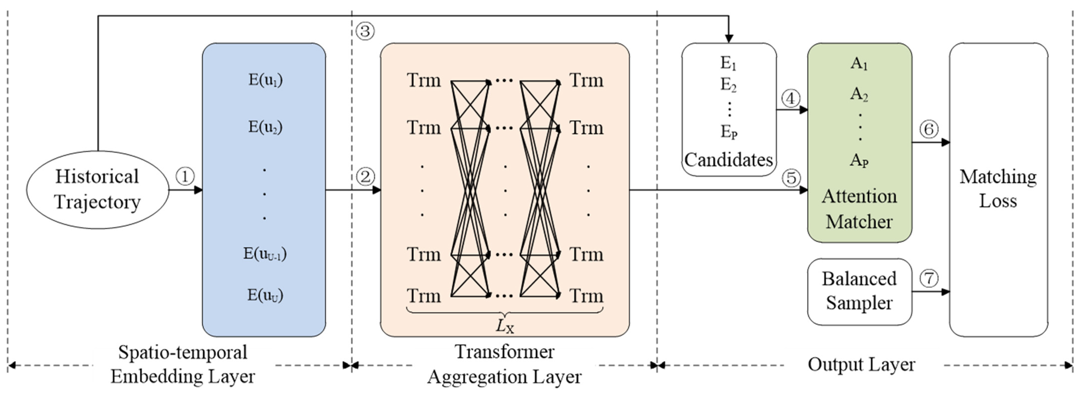
• We propose a multi-layer Spatio-Temporal attention model for the next location recommendation by mining the spatio-temporal relationship between visited locations (STTF-Recommender for short), including multi-layer Transformer aggregation and an attention matcher.
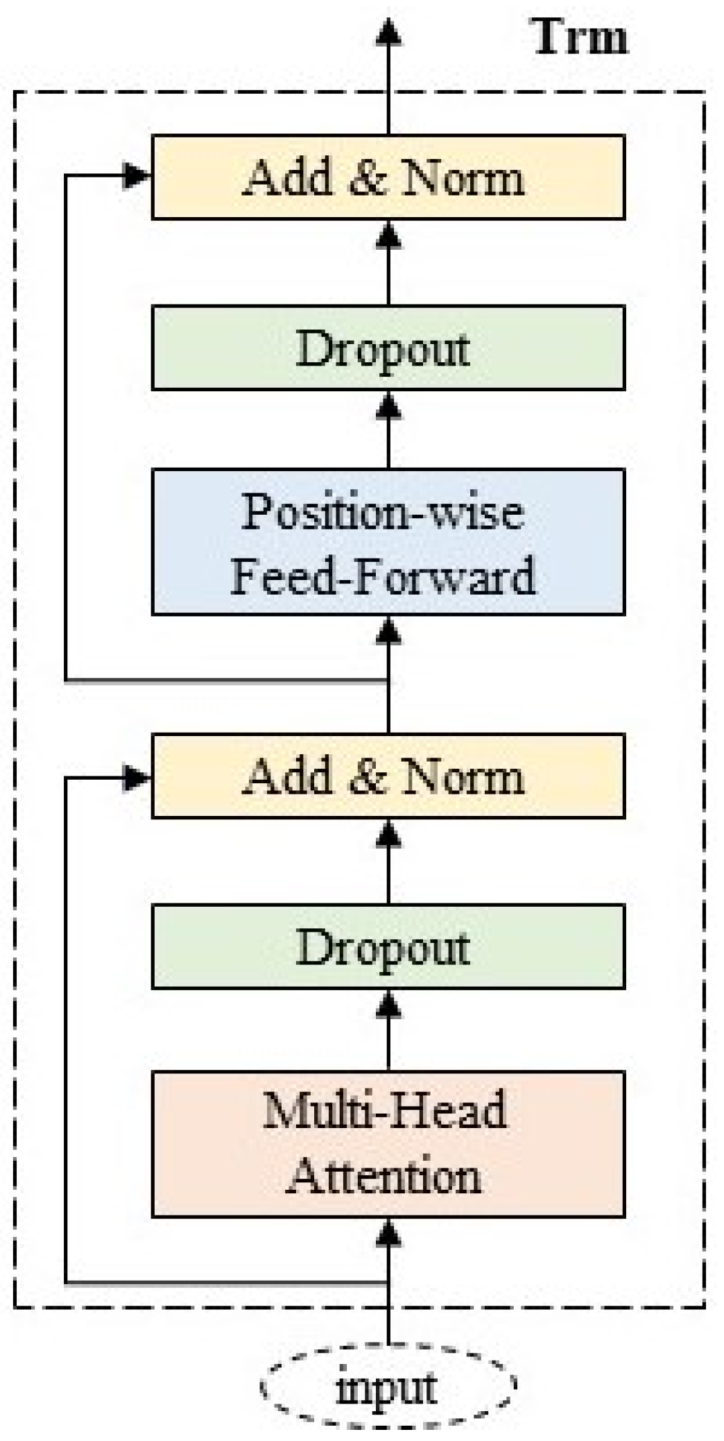
• We exploit the Transformer aggregation layer for processing sequence data, which can directly compute the correlation of two visits in a parallel way, and better capture long-term preferences in sequence data so that the patterns of non-adjacent locations and non-contiguous visits in LBSNs can be better discovered.
• We develop an attention matcher based on the attention mechanism by updating representations of check-in to match the most plausible candidate locations.
• We further explore the regularity of spatio-temporal in LBSN by constructing different aggregation modules to make a personalized recommendation. Consequently, the accuracy of recommendations can be further improved.
• We evaluate the performance of our model on two real data sets, including NYC [8] and Gowalla [9]. The results show that our model improves by at least 13.75% in the mean value of the Recall index at different scales compared with the state-of-the-art models and outperforms the best baseline by 4% in the Recall rate.

2. Related Works

In Section 2.1, we briefly review the related work of sequential recommendation, which is mainly to mine patterns in user interaction sequences. Next POI recommendation is an important branch of sequential recommendation, which will be described in Section 2.2.

2.1. Sequential Recommendation

Early work on sequential recommendation mainly employs Markov Chains (MCs) to capture sequential patterns from users’ historical interactions. For example, Shani et al. [13] formalized the recommendation result as a sequence optimization problem and addressed it by using Markov Decision Processes (MDPs). Later, Rendle et al. [14] combined the functions of MCs and Matrix Factorization (MF), sequence behavior, and general interests are modeled by Factorizing Personalized Markov Chains (FPMC). In addition to first-order MCs, higher-order MCs can consider more user previous activities for recommendation [15].

Recently, RNN and its variants, such as Gated Recurrent Unit (GRU) [16] and Long Short-Term Memory (LSTM) [17], have been increasingly applied in the modeling of user behavior sequences. The basic idea of these methods is to encode the user’s historical records into a vector to represent the user’s preferences for prediction. These methods include various recurrent architectures and loss functions, such as session-based GRU (GRU4Rec) [18], Dynamic REcurrentbAsket Model (DREAM) [19], etc., as well as new loss functions (such as BPR-max and TOP1-max) and improved sampling strategy. In addition to RNN, many other deep learning models have also been introduced into a sequential recommendation, such as CNN, Graph Neural Network (GNN), etc.

The attention mechanism shows great potential in sequence data modeling and has made considerable achievements in image classification and text processing. Recently, some researchers have attempted to utilize attention mechanisms to improve the performance and interpretability of recommendation models. For example, Li et al. [20] incorporate an attention mechanism into GRU to capture the continuous behavior and preferences of users in session-based recommendations. However, the sequence recommendation method mentioned above is not designed for the Next POI recommendation and ignores the spatio-temporal relationship in the LBSNs data sequence.

2.2. Next POI Recommendation

The Next POI recommendation techniques evolve with the development of sequential recommendation methods. Early Next POI recommendation models were mainly based on feature engineering and non-deep learning-based models, such as the Markov Chain model, Matrix Factorization (MF) model, etc. [21,22,23,24,25,26]. While having been extensively studied [21], stochastic models based on Markov chains are difficult to model non-contiguous POI visits generated from LBSNs due to the sparsity of such datasets. Subsequently, a model based on MF [22] was proposed and solved this problem. The MF model was used for modeling the Next POI recommendation [23]. In order to obtain better performance, some researchers adopted the Bayesian personalized classification (BPR) model [24]. Other non-deep learning-based models, such as support vector machine (SVM) [25], Collaborative Filtering [26], Gaussian Modeling [27], and Transitive Dissimilarity, have been also used for personalized Next POI recommendations in various works. However, all of these models rely on handcrafted features, which require sufficient domain expertise. With the unprecedented increase of LBSNs data, however, it becomes more difficult to design and extract data features. In recent years, the deep learning-based model can automatically extract features and therefore gradually replace most traditional models.

Deep learning-based models, such as CNN or RNN, perform well in automatic feature extraction and eliminate the difficulty of handcrafted feature design. In addition, the deep learning-based approach excelled in modeling the relationships between structured and unstructured data, which helped automatically extract data features in the Next POI recommendation. In the past few years, many efforts have been committed to the Next POI recommendation based on deep learning techniques, especially at some top computing conferences, such as the AAAI Conference on Artificial Intelligence (AAAI) and Proceedings of the ACM Web Conference (WWW) [7]. Different deep learning techniques, such as CNN, RNN, LSTM, and GRU, greatly improved the performance of the Next POI recommendation model.

Attention mechanism [12] is a practical technique widely used in artificial intelligence and deep learning tasks. The attentional mechanism improves the accuracy of the model by imitating human behavior and making the model focus dynamically on the information in the input data, which is helpful to the current machine learning task, and therefore can largely solve the problem of missing features in the long sequences [3]. The self-attention mechanism is also used in the Next POI recommendation system [8,28], which not only improves the performance of the model but also allows parallel processing of input. However, in the task of spatio-temporal data processing and the Next POI recommendation, previous models did not consider well the spatio-temporal relationship between non-adjacent locations and non-contiguous visits. Models, such as TMCA [29], capture spatial and temporal dependencies [3] among historical check-in activities by using LSTM [17] and three types of attention [30]. However, these models have not explored the potential of the attention mechanism. As such, the recommendation accuracy and recall rate of these models were still low. Alternatively, GT-HAN [31,32] captures great variation in geographical influence in the check-in list by using Bi-LSTM [33] and the attention mechanism. Our STTF-Recommender learns more complex spatio-temporal patterns by stacking Transformer layers and directly calculates the correlation between two visits, and therefore better mine and leverage the spatial-temporal relationship between non-adjacent locations and non-contiguous visits of user trajectory sequence for much-improved model performance.

3. Preliminaries

This section provides basic concepts and problem definitions, the main notation are shown in

Table 1. Table of main notation.

Notation	Description
$u_i$	User $i$
$p_k$	Location of Check-in $k$
$t_k$	Time of Check-in $k$
$r_k$	Check-in $k$, which is represented as a tuple $r_k=\left\{u_i,p_k,t_k\right\}$
$seq(u_i)$	trajectories sequence of $u_i$
$e^{\ast }$	The dense vectors of $\ast$
$E(\ast )$, $E_{\ast }$	Set of $e^{r_j}$, $r_j\in seq(\ast )$
$l$, $L$	A random layer, and number of layers
$h_i^l$	Hidden representations of visit $i$ in the layer $l$
$H^l$	A matrix of $h_i^l$ stacks
$\mathrm{Q}$, $K$, $V$	Query, keys, values [12]
$h$	Number of head
$hea{d}_i$	Projection matrices of each head, $i\in \left[1,h\right]$
$W_i^Q$	Projections matrices for $hea{d}_i$
$A\left(u\right)$, $A_i$	The probability set that each candidate location becomes the next location for user $u_i$

. We denote the set of user, location, and time as: $U=\left\{u_1,u_2\dots u_U\right\}$, $P=\left\{p_1,p_2\dots p_P\right\}$, $T=\left\{t_1,t_2\dots t_T\right\}$.

3.1. User Trajectory

The trajectory of a user $u_i$ is temporally ordered check-ins. Each check-in $r_k^{}$ of the user $u_i$ is represented as a tuple $r_k^{}=\left\{u_i,p_k,t_k\right\}$, where $p_k,t_k$ is the location and timestamp of the check-in, respectively. Each user $u_i$ may have a variable-length trajectory $tra(u_i)=\left\{r_1,r_2\dots r_{m_i}\right\}$, and $m_i$ is the trajectory length of user $u_i$. Inactive users with too few check-ins (less than 10) are discarded. Next, we transform each trajectory into a fixed-length sequence $seq(u_i)=\left\{r_1,r_2\dots r_n\right\}$, with $n$ as the maximum length we consider. If $m_i>n$, we only consider the most recent $n$ check-ins. If $m_i<n$, we pad 0 to the right until the sequence length is $n$ and mask off the padding items during calculation.

3.2. Definition of Problem Mobility Prediction

Given the user trajectory $\left(r_1,r_2\cdots r_m\right)$ and the location candidates $P=\left\{p_1,p_2\dots p_P\right\}$, our goal is to find the desired output $p\in r_{m+1}$.

4. The STTF-Recommender Model

This section will detail STTF-Recommender, which makes recommendations according to the user trajectory sequence. As shown in Figure 2, the model is mainly divided into three layers with seven steps, from ① to ⑦ (As for the specific parameters of the model, please refer to Section 5.1.3. In this section, we will focus on the structural design of the model):

4.1. Spatio-Temporal Embedding Layer

Built upon the spatio-temporal trajectory embedding method in the STAN model [8], a Spatio-Temporal Self-Attention Network for the next location recommendation, we designed our user trajectory embedded layer. The STAN model consists of four components: the first component, a multi-modal embedding module that learns the dense representations of user, location, time, and spatio-temporal relationship; the second component, a self-attention aggregation layer that aggregates important relevant locations within the user trajectory to update the representation of each check-in; the third component, an attention matching layer that calculates softmax probability from weighted check-in representations to compute the probability of each location candidate for next location; the fourth component, a balanced sampler that use a positive sample and several negative samples to compute the cross-entropy loss. In this spatio-temporal embedding layer, the user, location, and time in the trajectory are encoded into latent representations as $e^u\in {ℝ}^d,e^p\in {ℝ}^d,e^t\in {ℝ}^d$, respectively, and transform the scalars into dense vectors to reduce computation and improve representation. We divide the continuous timestamp into $7\times 24=168$ h to represent the exact time of the week, which maps the original time to 168 dimensions. This time division reflects the periodicity of the trajectory (Section 5.3 will discuss the impact of different time decomposition methods). The output of the user trajectory embedding layer for each check-in $r$ is the sum $e^r=e^u+e^p+e^t\in {ℝ}^d$. For the embedding of each user trajectory sequence $seq(u_i)=\left\{r_1,r_2\dots r_n\right\}$, we denote as $E(u_i)=\left\{e^{r_1},e^{r_2},\dots ,e^{r_n}\right\}\in {ℝ}^{n\times d}$. The corresponding input dimensions of the embedding $e^u,e^p,e^t$ are $U,P,168$.

4.2. Transformer Aggregation Layer

Inspired by BERT4Rec [11], we built a Transformer aggregation layer to consider spatio-temporal patterns and update the representation of each visit. We input the user trajectories sequence $E(u)\in {ℝ}^{n\times d}$ into the Transformer layer as a starting layer $H^0$. Next, we iterate the hidden representations $h_i^l$ of each visit $e^{r_i}$ simultaneously on the layer $l$, and then stack $h_i^l\in {ℝ}^d$ together into a matrix $H^l\in {ℝ}^{n\times d}$ to compute the attention functions at all positions simultaneously and capture long-term dependencies [11]. We set the layer number $L$ = 2, and conduct comparative experiments with different numbers of $L$ in Section 5.3. This layer is divided into two sub-layers: multi-head self-attention network sub-layer and the position feedforward network sub-layer. We abbreviate each Transformer unit structure to $Trm$, as shown in Figure 3.

Multi-Head Self-Attention: The attention mechanism pays attention to the input weight, which can capture the dependencies from different representation subspaces at different positions without considering the distance limit between representation pairs in the sequence. Specifically, we first linearly project $H^l$ into $h$ subspaces with different learnable linear projections, then apply $h$ attention functions to generate outputs in parallel, and then re-connect these outputs to generate output representations. We set the head number $h$ = 8 as long sequence datasets to benefit from a larger $h$ [12].

$$\begin{array}{l}MH\left(H^l\right)=\left[hea{d}_1;hea{d}_2;\dots ;hea{d}_h\right]W^O\\ hea{d}_i=Attention\left(H^l{W}_i^Q,H^l{W}_i^K,H^l{W}_i^V\right)\end{array}$$

(1)

where $hea{d}_i$ denotes the projection matrices of each $hea{d}_i$ $i\in \left[1,h\right]$, $W_i^Q\in {ℝ}^{d\times d/h}$, $W_i^K\in {ℝ}^{d\times d/h}$, $W_i^V\in {ℝ}^{d\times d/h}$, are learnable parameters. The attention function is the Scaled Dot-Product Attention:

$$Attention\left(Q,K,V\right)=softmax\left(\frac{Q{K}^{\top }}{\sqrt{d/h}}\right)V$$

(2)

where $Q,K,V$ are projected from the same matrix $H^l$ with different learned projection matrices, and the temperature $\sqrt{d/h}$ is introduced to avoid extremely small gradients [12].

Position-wise Feed-Forward Network: As mentioned above, the self-attention sub-layer is primarily based on linear projections. In order to make the model nonlinear and interactional between different dimensions, we apply a Position-wise Feed-Forward Network to the outputs of the self-attention layer separately and equally at each position. It consists of two affine transformations in which the Gaussian error linear unit ($GELU$) is activated:

$$\begin{array}{c}PFFN\left(H^l\right)={\left[FFN{\left(h_1^l\right)}^{\top };\dots ;FFN{\left(h_n^l\right)}^{\top }\right]}^{\top }\\ FFN\left(x\right)=GELU\left(x{W}^{\left(1\right)}+b^{\left(1\right)}\right)W^{\left(2\right)}+b^{\left(2\right)}\\ GELU\left(x\right)=x\mathsf{\Phi }\left(x\right)\end{array}$$

(3)

where $\mathsf{\Phi }\left(x\right)$ is the cumulative distribution functions of the standard Gaussian distribution, $W^{\left(1\right)}\in R^{\mathrm{d}\times 4\mathrm{d}},W^{\left(2\right)}\in R^{\mathrm{d}\times 4\mathrm{d}},b^{\left(1\right)}\in R^{4\mathrm{d}}$, and $b^{\left(2\right)}\in R^{\mathrm{d}}$ are learnable parameters that are shared across all locations.

The self-attention mechanism captures the check-in interaction across the entire user trajectory. Stacking the self-attention layer can better learn the transformation process during check-in interaction (see Section 5.3 for details) and learn more complex spatio-temporal patterns. However, as the network deepens, training becomes more difficult. Therefore, we use a residual connection around each of the two sub-layers and then perform layer normalization ($LN$). In addition, we apply Dropout to the output of each sub-layer before it is normalized. As such, the output of each sub-layer is $LN\left(x+Dropout(sublayer(x))\right)$, where the $sublayer(\cdot )$ is the function implemented by the sub-layer itself and $LN$ is the layer normalization function. We use $LN$ to normalize the input of all hidden cells in the same layer to stabilize and speed up network training.

In summary, the hidden representation of each layer $l$ is treated as follows:

$$\begin{array}{c}{H}^l=Trm\left(H^{l-1}\right),\forall i\in \left[1,\dots ,L\right]\\ Trm\left(H^{l-1}\right)=LN\left(A^{l-1}+Dropout\left(PFFN\left(A^{l-1}\right)\right)\right)\\ A^{l-1}=LN\left(H^{l-1}+Dropout\left(MH\left(H^{l-1}\right)\right)\right)\end{array}$$

(4)

where the $A^{l-1}$ is the output of sub-layer Multi-Head Self-Attention, the $H^l=Trm\left(H^{l-1}\right)$ is the output of sub-layer Position-wise Feed-Forward Network, i.e., the output of layer $l$.

4.3. Output Layer

This layer is divided into two parts, an attention matcher and a balance sampler. The attention matcher selects the most reasonable candidate locations, and the balance sampler solves the imbalance of positive and negative sample sizes.

Attention matcher: This part is based on the attention mechanism, which can select the most reasonable candidate locations from all potential locations by updating the representation that matches the user trajectory. According to the updated trajectory representation $S\left(u\right)=H^L\in R^{n\times d}$ in Section 4.2 and the recommendation of candidate locations $E\left(p\right)=\left\{e_1^p,e_2^p,\dots ,e_P^p\right\}$, the probability that each candidate location in this layer becomes the next location is shown as follows:

$$A\left(u\right)=Matching\left(E\left(p\right),S\left(u\right)\right)$$

(5)

Among them:

$$Matching\left(Q,K\right)=Sum\left(soft\max \left(\frac{Q{K}^{\top }}{\sqrt{d}}\right)\right)$$

(6)

Here, the $Sum$ operation is a weighted sum of the last dimension, converting the dimension of $A\left(u\right)$ to be $R^P$. All the updated representations of check-ins participate in the matching of each candidate location, as shown in Equation (5).

Balanced sampler: Due to the imbalance scale of positive and negative sample sizes in $A\left(u\right)$, the optimization of cross-entropy loss is no longer effective. General cross-entropy loss for each positive sample $a_k$ needs to calculate $P-1$ negative samples, which will lead to an imbalance problem. As such, we only use random $ne$ negative samples for each calculation, where $ne$ is a hyperparameter we set to 10.

Given the sequence $seq\left(u_i\right)$ of users $i$, for the matching probability $a_j\in A\left(u_i\right)$ of each location $j\in \left[1,P\right]$, the cross-entropy loss of labels $k$ in the location set $P$ is written as:

$$-\sum _i{\displaystyle \sum _{m_i}\left(\log \sigma (a_k+{\displaystyle \sum _{(j_1,j_2\mathrm{...}{j}_{ne})\in [1,P],j_i\ne k}\log \left(1-\sigma \left(a_j\right)\right)}\right)}$$

(7)

where $m_i$ is the length of user $u_i$ trajectory and other symbols are defined as before.

5. Performance Evaluation

This section presents the experimental design and empirical results of our model to make it fairly compared with other models. We present a table of our experimental data set and a table of the comparative results at the Top@k recall rate. In addition, we also conduct an ablation study on key components of our model to demonstrate the effectiveness of these key components.

5.1. Experiment

This section introduces our experimental setup, including the data set, baseline models, and model implementation details.

5.1.1. Datasets

We evaluated the models on two real datasets as

Table 2. Basic dataset statistics.

Dataset	User	POIs	Check-Ins
Gowalla	10,162	24,250	456,988
NYC	1064	5136	147,939

shown: The Gowalla dataset [9], and the NYC dataset [8]. First, we preprocess each dataset to filter out trajectories with invalid time and place, and only select users whose check-in sequence length is greater than five for the experiment. According to the previous research 8, the experiment is divided into training, validation, and test datasets. For each user who has $m$ check-in, the length of the training set is $m-3$. The first $m^{\prime }\in \left[1,m-3\right]$ check-in data are used as input, and the $[2,m-2]-nd$ check-in data are used as labels; the validation set uses the first $m-2$ check-ins as input, the $\left(m-1\right)-st$ check-in data as a label; the test set uses the first $m-1$ check-ins as input and the $m-th$ check-in data as the label.

5.1.2. Baseline Models

We compared our model with several baseline models below.

• STRNN [9]: A RNN model with invariance, which incorporates spatio-temporal features among consecutive visits.
• LSTPM [7]: A model based on LSTM. It uses two LSTMS to capture users’ long- and short-term preferences and uses geographic extended RNN to simulate discontinuous geographic relationships among POIS.
• DeepMove [10]: A prediction model that uses GRU to deal with short-term dependence and attention to capture historical activities.
• STAN [8]: A model using a self-attention mechanism to deal with spatio-temporal data relation.

5.1.3. Evaluation Method

To evaluate the proposed recommender, we first download and use the open-source codes of four baseline models. While running the proposed and baseline models, the embedding dimension, learning rate, dropout rate, and training period of the dataset are set to 50, 0.003, 0.2, and 50, respectively. Meanwhile, our model uses two Transformer layers with a dropout rate of 0.2, the head number $h$ is 8, the number of layers $L$ is 4, an embedded dimension of 50, an Adam optimizer, and a check-in sequence length of 100.

We use the TOP recall rate Recall@K, the probability that there are correct POIs in the first K recommended POIs, to evaluate the model recommendation performance. The closer the Recall@K is to 1, the better the effect. In the evaluation, we directly use the output results in the attention matcher module of the output layer for evaluation.

5.2. Results

We first compare our model with the baseline models.

Table 3. Recommendation Performance Comparison with Baselines.

	Gowalla		NYC
	Recall@5	Recall@10	Recall@5	Recall@10
STRNN [9]	0.16	0.25	0.24	0.28
LSTPM [7]	0.20	0.27	0.27	0.35
DeepMove [10]	0.19	0.26	0.32	0.40
STAN [8]	0.30	0.39	0.46	0.59
STTF-Recommender	0.35	0.43	0.53	0.65
Improvement	13.75%	13.75%	20.75%	24.5%

The Bold Entries Highlight Our Results.

shows that our model performs better than other baseline models at Recall@5 and Recall@10. Each model runs 10 times with different data sets as well as different tops, and we use the average performance of each model for evaluation. The results indicate that, at Recall@5 and Recall@10, our model is improved by at least 4% compared with the best baseline models, demonstrating the feasibility and effectiveness of our model.

In our baseline models, the performance of STRNN is significantly lower than that of other models. This is because the general RNN-based models can only capture short-term sequence rules and cannot capture long-term dependencies well. LSTPM is better than STRNN because it uses LSTM to model the user’s long-term trajectory and short-term trajectory, respectively. LSTPM considers the long-term preference, while it still cannot completely solve this problem. DeepMove takes long-term dependence into account and uses an attention mechanism to learn the periodicity of human activities in trajectory modeling, which also improves the model performance. STAN uses the double-layer attention structure to gather the spatio-temporal correlation of the track sequence, which solves the long-term dependence of the sequence to some extent, leading to better performance.

Our STTF-Recommender adopts a double-layer Transformer aggregation layer to aggregate the trajectory, which can directly calculate the correlation between the two visits without regard to their distance in the sequences. As such, it better captures the long-term dependence of sequences and improves the experimental performance. Compared with STAN, the results showed that our STTF-Recommender improved recommendation performance by about 5%. This is because our model employed both a multi-head attention layer and a location feed-forward network. In particular, multi-head attention allows the model to jointly attend to information from different representation subspaces at different positions, and the position-based feed-forward networks can also improve the performance of the model, as we show in Section 5.3 by performing experiments on the relevant components.

5.3. Ablation Study

We perform ablation experiments over the aggregation layer in order to better understand their impacts, and we designed five different variants of the STTF:

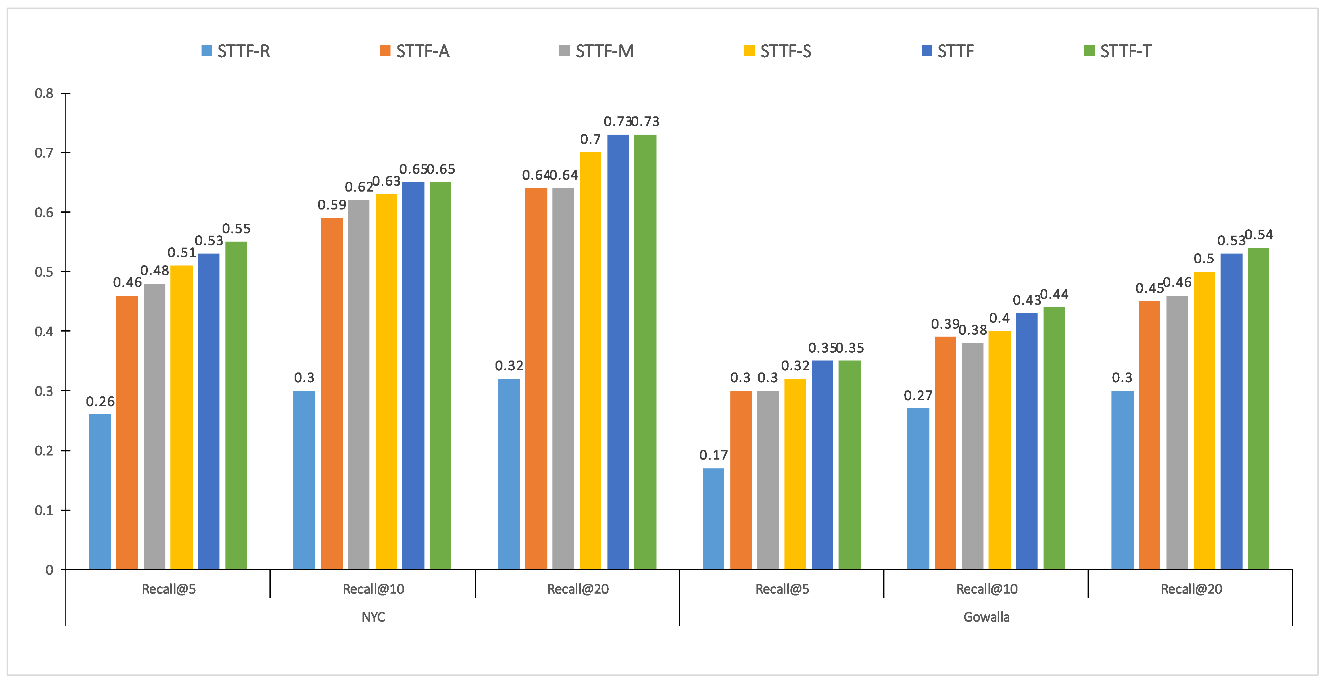
• STTF-R used recurrent layers as the aggregation layer, which only can model consecutive activities in the user’s check-in sequence while it cannot learn the features of discrete visits.
• STTF-A only used a self-attention as the aggregation layer, which can capture long-term dependency and assign different weights to each visit within the trajectory.
• STTF-M adopted the multi-head self-attention, which mapped the input to different subspaces through a random initialization to capture the dependencies from different representation subspaces.
• STTF-S used a single-layer transformer, which added Position-wise Feed-Forward Network over the STTF-M as the aggregation layer.
• STTF-T stacked three transformer layers, which investigated whether more transformer layers can further improve the recommendation performance.

Figure 4 illustrates the performance of the STTF compared to the five variants, and it was clear that the STTF performed better than most of its variants in the recall. STTF-R used recurrent layers as the aggregation layer, not effectively considering the correlations between non-adjacent locations and non-contiguous visits. STTF-A only used a self-attention as the aggregation layer. STTF-M adopted the multi-head self-attention and mapped the input to different subspaces through a random initialization, which can improve the model computation speed through parallel computing but can hardly improve the recommendation performance. The STTF-S used a single-layer transformer, which added a feedforward network sub-layer on the basis of a multi-head attention sub-layer. The single-layer transformer can automatically adjust each position in the sequence through feedforward and consequently yielded an increase of 8% on different recall@k. Considering Transformer networks can be multi-layered, we stacked a layer on top of a single Transformer layer to build STTF, and the results showed that this approach improved recommendation performance by about 5%, indicating that a deeper Transformer network facilitates learning data patterns. STTF-T stacked three transformer layers but did not achieve much improvement, and continued stacking would lead to overfitting.

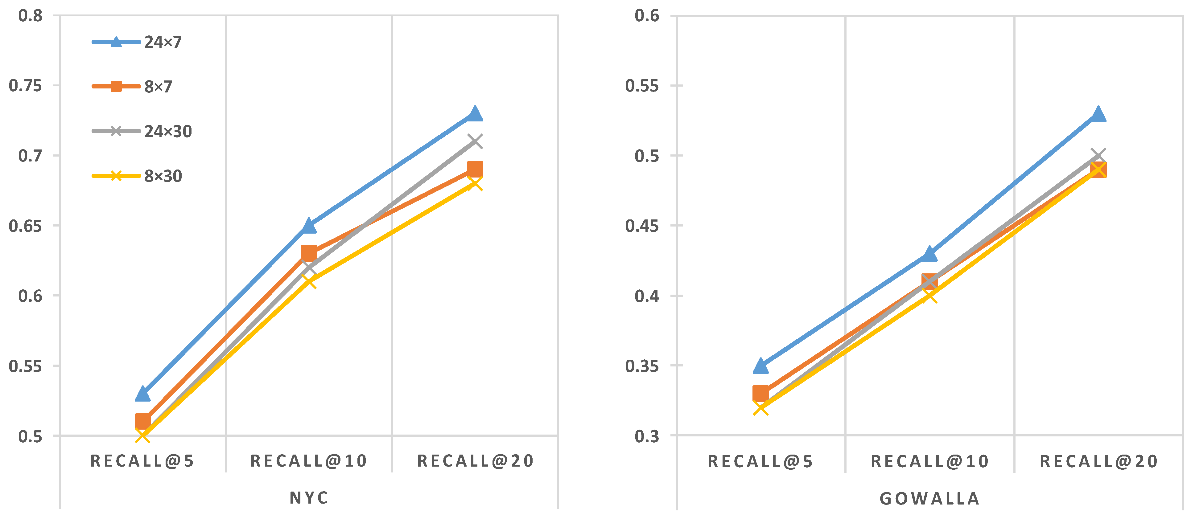
5.4. The Impact of Different Time Scale

In the previous experiment, time embedding was performed every hour of every week. To examine the impact of time embedding scales, we evaluated time embedding every three hours of every week, every three hours of every month, and every one hour of every month. The experimental results are shown in Figure 5, where 8 and 24 represent the calculation times of every day, and 7 and 30 represent the embedding cycle. The Rec@5 values of the 24 × 7, 8 × 7, 24 × 30, and 8 × 30 on the NYC dataset were 0.53, 0.51, 0.50, and 0.50, respectively. Three-hour intervals are more difficult to predict, and therefore the results of hour intervals are embedded better than those of three-hour intervals. Since most people have relatively regular movement patterns in terms of sequential cycles, the results of experiments on a monthly scale are not as good as those on a weekly scale.

6. Conclusions

In this paper, we study the recommendation of the next POI of users’ check-in in social networks and propose a spatio-temporal attention model based on deep learning, which uses a multi-layer attention network to compute the spatio-temporal relationship between non-adjacent locations and non-contiguous visits from the user trajectory sequence, and updates the representation of each visit that matches the user trajectory to make a personalized recommendation, as the Figure 6 shown. The performance of our model is evaluated on two real-world datasets (NYC and Gowalla). Experimental results demonstrate that the proposed STTF-Recommender is effective and significantly superior to existing methods.

Next, several future research directions can be explored. One direction is to incorporate rich influential factors that affect the Next POI recommendation (e.g., social influence, semantic information) into STTF. Another potential direction would be to introduce spatial distances to reflect the spatial preferences of users.

References

1. Huang, Q.; Wong, D.W.S. Activity patterns, socioeconomic status and urban spatial structure: What can social media data tell us? Int. J. Geogr. Inf. Sci. 2016, 30, 1873–1898. [Google Scholar] [CrossRef]
2. Xu, S.; Fu, X.; Cao, J.; Liu, B.; Wang, Z. Survey on user location prediction based on geo-social networking data. World Wide Web 2020, 23, 1621–1664. [Google Scholar] [CrossRef]
3. Islam, A.; Mohammad, M.M.; Das, S.S.S.; Ali, M.E. A survey on deep learning based Point-of-Interest (POI) recommendations. Neurocomputing 2021, 472, 306–325. [Google Scholar] [CrossRef]
4. Zou, Z.; Xie, X.; Sha, C. Mining User Behavior and Similarity in Location-Based Social Networks. In Proceedings of the 2015 Seventh International Symposium on Parallel Architectures, Algorithms and Programming (PAAP), Nanjing, China, 12–14 December 2015; pp. 167–171. [Google Scholar] [CrossRef]
5. Wang, S.; Cao, J.; Yu, P.S. Deep Learning for Spatio-Temporal Data Mining: A Survey. IEEE Trans. Knowl. Data Eng. 2020, 34, 3681–3700. [Google Scholar] [CrossRef]
6. Yang, X.; Guo, Y.; Liu, Y.; Steck, H. A survey of collaborative filtering based social recommender systems. Comput. Commun. 2014, 41, 1–10. [Google Scholar] [CrossRef]
7. Sun, K.; Qian, T.; Chen, T.; Liang, Y.; Nguyen, Q.V.H.; Yin, H. Where to Go Next: Modeling Long- and Short-Term User Preferences for Point-of-Interest Recommendation. In Proceedings of the AAAI Conference on Artificial Intelligence, New York, NY, USA, 7–12 February 2020; Volume 34, pp. 214–221. [Google Scholar] [CrossRef]
8. Luo, Y.; Liu, Q.; Liu, Z. STAN: Spatio-Temporal Attention Network for Next Location Recommendation. In Proceedings of the Web Conference 2021, Ljubljana, Slovenia, 19–23 April 2021; Volume 2021, pp. 2177–2185. [Google Scholar] [CrossRef]
9. Liu, Q.; Wu, S.; Wang, L.; Tan, T. Predicting the Next Location: A Recurrent Model with Spatial and Temporal Contexts. In Proceedings of the AAAI Conference on Artificial Intelligence, Phoenix, AZ, USA, 12–17 February 2021; Volume 30, pp. 194–200. [Google Scholar] [CrossRef]
10. Feng, J.; Li, Y.; Zhang, C.; Sun, F.; Meng, F.; Guo, A.; Jin, D. Deepmove: Predicting Human Mobility with Attentional Recurrent Networks. In Proceedings of the 2018 World Wide Web Conference, Lyon, France, 23–27 April 2018; Volume 2, pp. 1459–1468. [Google Scholar]
11. Sun, F.; Liu, J.; Wu, J.; Pei, C.; Lin, X.; Ou, W.; Jiang, P. BERT4Rec: Sequential Recommendation with Bidirectional Encoder Representations from Transformer. In Proceedings of the 28th ACM International Conference on Information and Knowledge Management, Beijing, China, 3–7 November 2019. [Google Scholar]
12. Vaswani, A.; Shazeer, N.; Parmar, N.; Uszkoreit, J.; Jones, L.; Gomez, A.N.; Kaiser, Ł.; Polosukhin, I. Attention is all you need. In Proceedings of the Advances in Neural Information Processing Systems 30 (NIPS 2017), Long Beach, CA, USA, 4–9 December 2019; Volume 30. [Google Scholar]
13. Shani, G.; Heckerman, D.; Brafman, R.I. An MDP-based recommender system. J. Mach. Learn. Res. 2005, 6. [Google Scholar]
14. Rendle, S.; Freudenthaler, C.; Schmidt-Thieme, L. Factorizing personalized Markov chains for next-basket recommen-dation. In Proceedings of the 19th International World Wide Web Conference, Raleigh, NC, USA, 26–30 April 2010. [Google Scholar]
15. He, R.; Kang, W.-C.; McAuley, J. Translation-based Recommendation. In Proceedings of the Translation-Based Recommendation, Como, Italy, 27–31 August 2017; ACM: New York, NY, USA, 2017; pp. 161–169. [Google Scholar]
16. Cho, K.; van Merriënboer, B.; Gulcehre, C.; Bahdanau, D.; Bougares, F.; Schwenk, H.; Bengio, Y. Learning Phrase Representations Using RNN Encoder-Decoder for Statistical Machine Translation. In Proceedings of the 2014 Conference on Empirical Methods in Natural Language Processing (EMNLP), Doha, Qatar, 25–29 October 2014; pp. 1724–1734. [Google Scholar]
17. Hochreiter, S.; Schmidhuber, J. Long short-term memory. Neural Comput. 1997, 9, 1735–1780. [Google Scholar] [CrossRef] [PubMed]
18. Hidasi, B.; Karatzoglou, A.; Baltrunas, L.; Tikk, D. Session-based recommendations with recurrent neural networks. arXiv 2016, arXiv:1511.06939. [Google Scholar]
19. Donkers, T.; Loepp, B.; Ziegler, J. Sequential User-based Recurrent Neural Network Recommendations. In Proceedings of the Eleventh ACM Conference on Recommender Systems, Como, Italy, 27–31 August 2017; pp. 152–160. [Google Scholar] [CrossRef]
20. Li, J.; Wang, Y.; McAuley, J. Time Interval Aware Self-Attention for Sequential Recommendation. In Proceedings of the Thirteenth ACM International Conference on Web Search and Data Mining, Houston, TX, USA, 3–7 February 2020. [Google Scholar] [CrossRef] [Green Version]
21. Noulas, A.; Scellato, S.; Mascolo, C.; Pontil, M. Exploiting semantic annotations for clustering geographic areas and users in location-based social networks. AAAI Work.-Tech. Rep. 2011, WS-11-02, 32–35. [Google Scholar]
22. He, J.; Li, X.; Liao, L.; Wang, M. Inferring continuous latent preference on transition intervals for next point-of-interest recommendation. In Lecture Notes in Computer Science (including subseries Lecture Notes in Artificial Intelligence and Lecture Notes in Bioinformatics); Proceedings, Part II 18; Springer International Publishing: Berlin/Heidelberg, Germany, 2019; Volume 11052 LNAI. [Google Scholar]
23. Liu, W.; Wang, Z.J.; Yao, B.; Nie, M.; Wang, J.; Mao, R.; Yin, J. Geographical relevance model for long tail point-of-interest recommendation. In Lecture Notes in Comput-er Science (including subseries Lecture Notes in Artificial Intelligence and Lecture Notes in Bioinformatics); Springer: Cham, Switzerland, 2018; Volume 10827 LNCS. [Google Scholar]
24. Baral, R.; Iyengar, S.S.; Zhu, X.; Li, T.; Sniatala, P. HiRecS: A Hierarchical Contextual Location Recommendation System. IEEE Trans. Comput. Soc. Syst. 2019, 6, 1020–1037. [Google Scholar] [CrossRef]
25. Huang, Q.; Li, Z.; Li, J.; Chang, C. Mining frequent trajectory patterns from online footprints. In Proceedings of the 7th ACM SIGSPATIAL International Workshop on GeoStreaming, San Francisco, CA, USA, 31 October 2016; pp. 1–7. [Google Scholar]
26. Li, J.; Liu, G.; Yan, C.; Jiang, C. Lori: A learning-to-rank-based integration method of location recommendation. IEEE Trans. Comput. Soc. Syst. 2019, 6, 430–440. [Google Scholar] [CrossRef]
27. Yang, D.; Fankhauser, B.; Rosso, P.; Cudre-Mauroux, P. Location Prediction over Sparse User Mobility Traces Using RNNs. In Proceedings of the Twenty-Ninth International Joint Conference on Artificial Intelligence, Yokohama, Japan, 11–17 July 2020; pp. 2184–2190. [Google Scholar] [CrossRef]
28. Halder, S.; Lim, K.H.; Chan, J.; Zhang, X. Transformer-based multi-task learning for queuing time aware next POI rec-ommendation. In Pacific-Asia Conference on Knowledge Discovery and Data Mining: 25th Pacific-Asia Conference, PAKDD 2021, Virtual Event, 11–14 May 2021; Springer International Publishing: Cham, Switzerland, 2021; pp. 510–523. [Google Scholar]
29. Li, R.; Shen, Y.; Zhu, Y. Next Point-of-Interest Recommendation with Temporal and Multi-level Context Attention. In Proceedings of the 2018 IEEE International Conference on Data Mining (ICDM), Singapore, 17–20 November 2018; pp. 1110–1115. [Google Scholar] [CrossRef]
30. Qin, Y.; Song, D.; Chen, H.; Cheng, W.; Jiang, G.; Cottrell, G.W. A dual-stage attention-based recurrent neural network for time series prediction. IJCAI 2017, 2627–2633. [Google Scholar]
31. Liu, T.; Liao, J.; Wu, Z.; Wang, Y.; Wang, J. Exploiting geographical-temporal awareness attention for next point-of-interest recommendation. Neurocomputing 2020, 400, 227–237. [Google Scholar] [CrossRef]
32. Liu, T.; Liao, J.; Wu, Z.; Wang, Y.; Wang, J. A Geographical-Temporal Awareness Hierarchical Attention Network for Next Point-of-Interest Recommendation. In Proceedings of the International Conference on Multimedia Retrieval, Ottawa, ON, Canada, 10–13 June 2019; pp. 7–15. [Google Scholar] [CrossRef]
33. Liu, C.H.; Wang, Y.; Piao, C.; Dai, Z.; Yuan, Y.; Wang, G.; Wu, D. Timeaware location prediction by convolutional area-of-interest modeling and memory-augmented attentive lstm. IEEE Trans. Knowl. Data Eng. 2020, 34, 2472–2484. [Google Scholar] [CrossRef]
Figure 1. Examples of trajectories showing the relation between non-consecutive visits and non-adjacent locations, the markers 1 through 5 are the most frequently visited locations by a user.
Ijgi 12 00079 g001
Figure 2. The framework of the proposed STTF-Recommender. Spatio-Temporal embedding layer is used to encode user, location, and time from the historical trajectory into latent representations ①. Transformer aggregation layer is exploited to gather the locations of visits ② and update the hidden representation of each visit by stacking the Transformer layers so that our model can better mine the spatio-temporal relationship between non-adjacent locations and non-contiguous visits in the user trajectory sequence. Output layer is further divided into two modules: attention matcher and balance sampler, where attention matcher calculates the probability of each candidate location becoming the next visit location according to candidate location③, ④ and hidden representation of each visit ⑤. The balance sampler then calculates the cross-entropy loss using one positive sample and multiple negative samples⑥, ⑦.
Ijgi 12 00079 g002
Figure 3. Transformer unit structure.
Ijgi 12 00079 g003
Figure 4. Ablation Analysis by Comparing Different Modules in STTF-Recommender.
Ijgi 12 00079 g004
Figure 5. The Impact of Different Time Scales.
Ijgi 12 00079 g005
Figure 6. The sample map shows a sequence of locations that our model outputs. By examining the exact location in the Google Map, we found that location 2 is the New York Academy of Photography, other locations are very suitable for photography, for example, locations 1, 3, and 4 are parks, and location 5 is a Fine Arts Gallery. Although these locations are not adjacent to each other on the map, our model exploits the correlation between these locations.
Ijgi 12 00079 g006