
Mechanical Design of a Biped Robot FORREST and an Extended Capture-Point-Based Walking Pattern Generator

Abstract
:1. Introduction
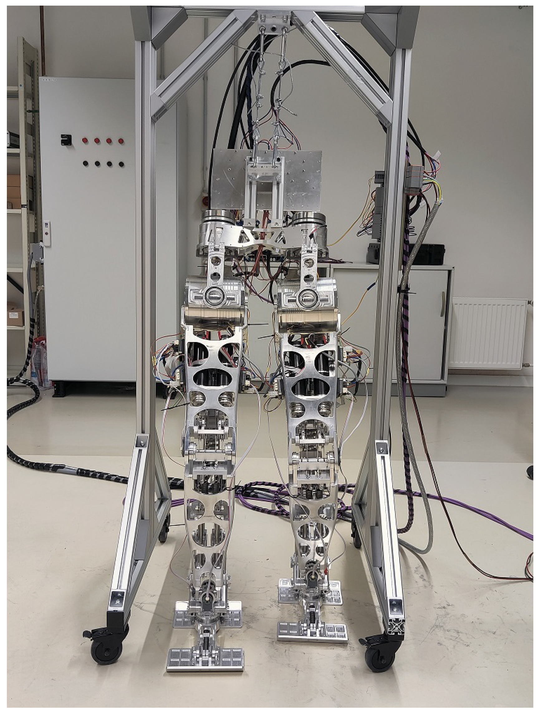
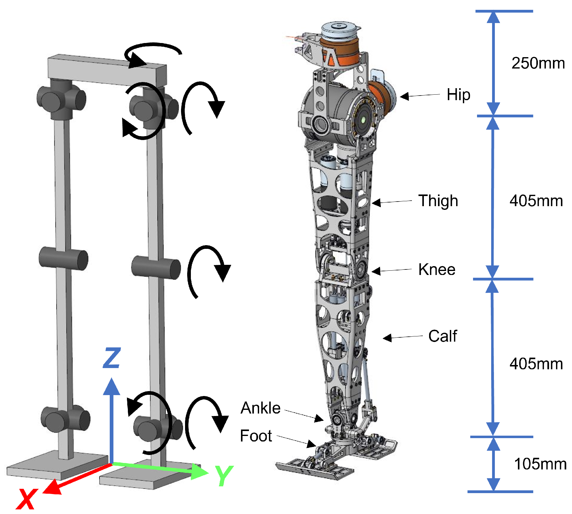
2. Overview of FORREST’s Design
3. Design of the New Biped Robot
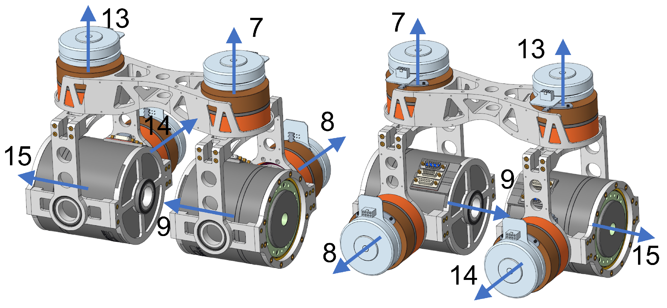
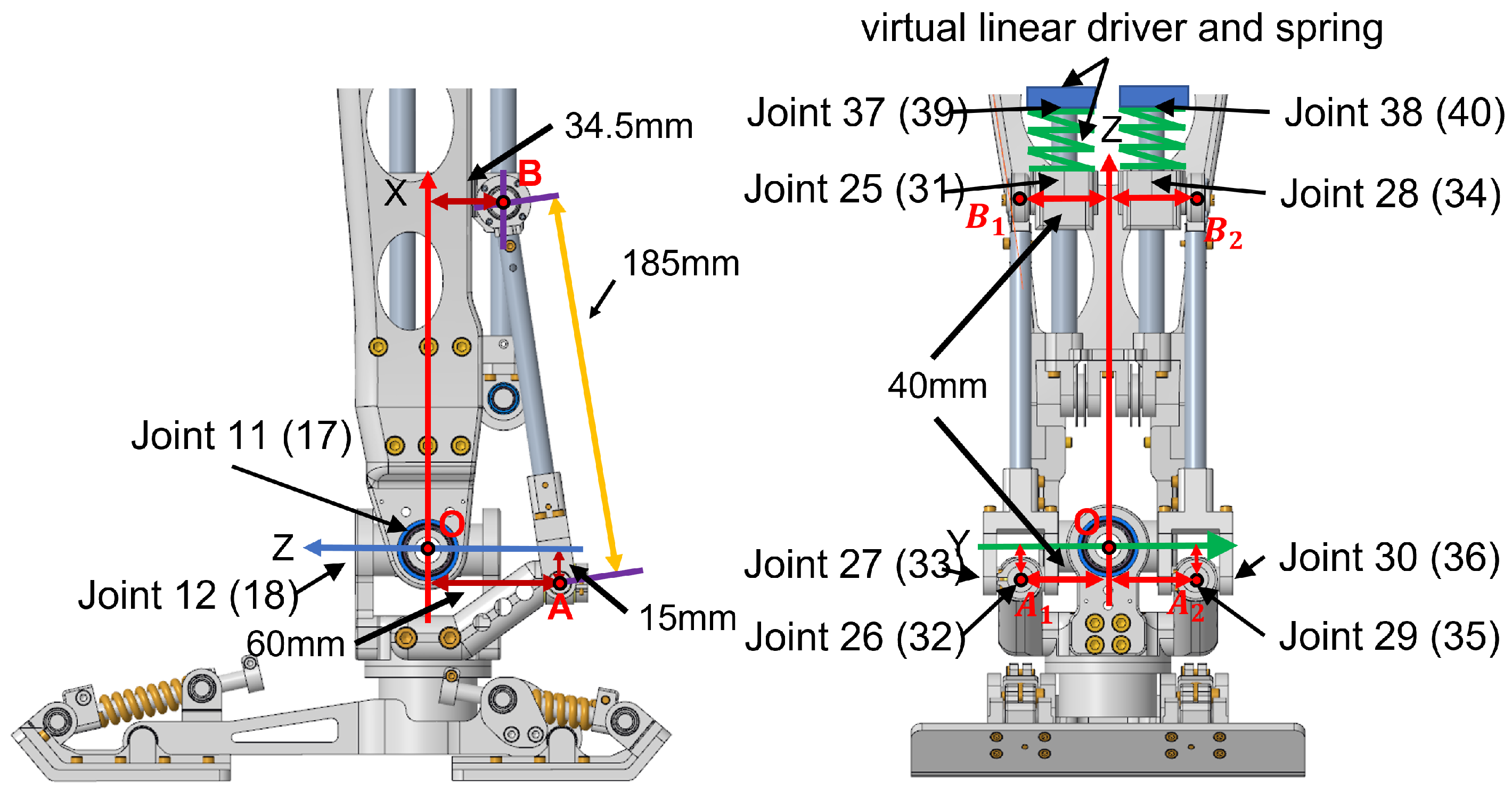
3.1. Hip
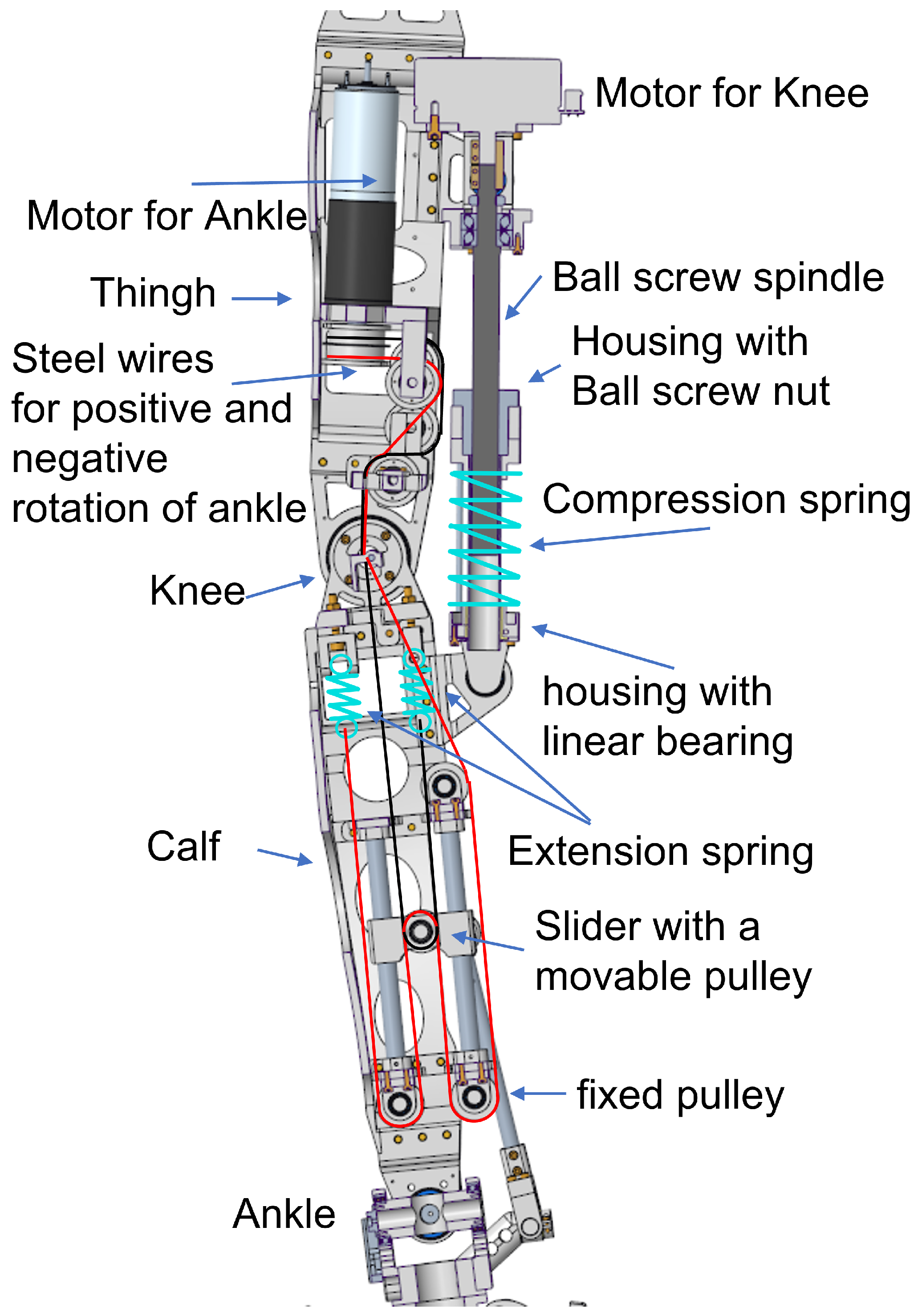
3.2. Knee
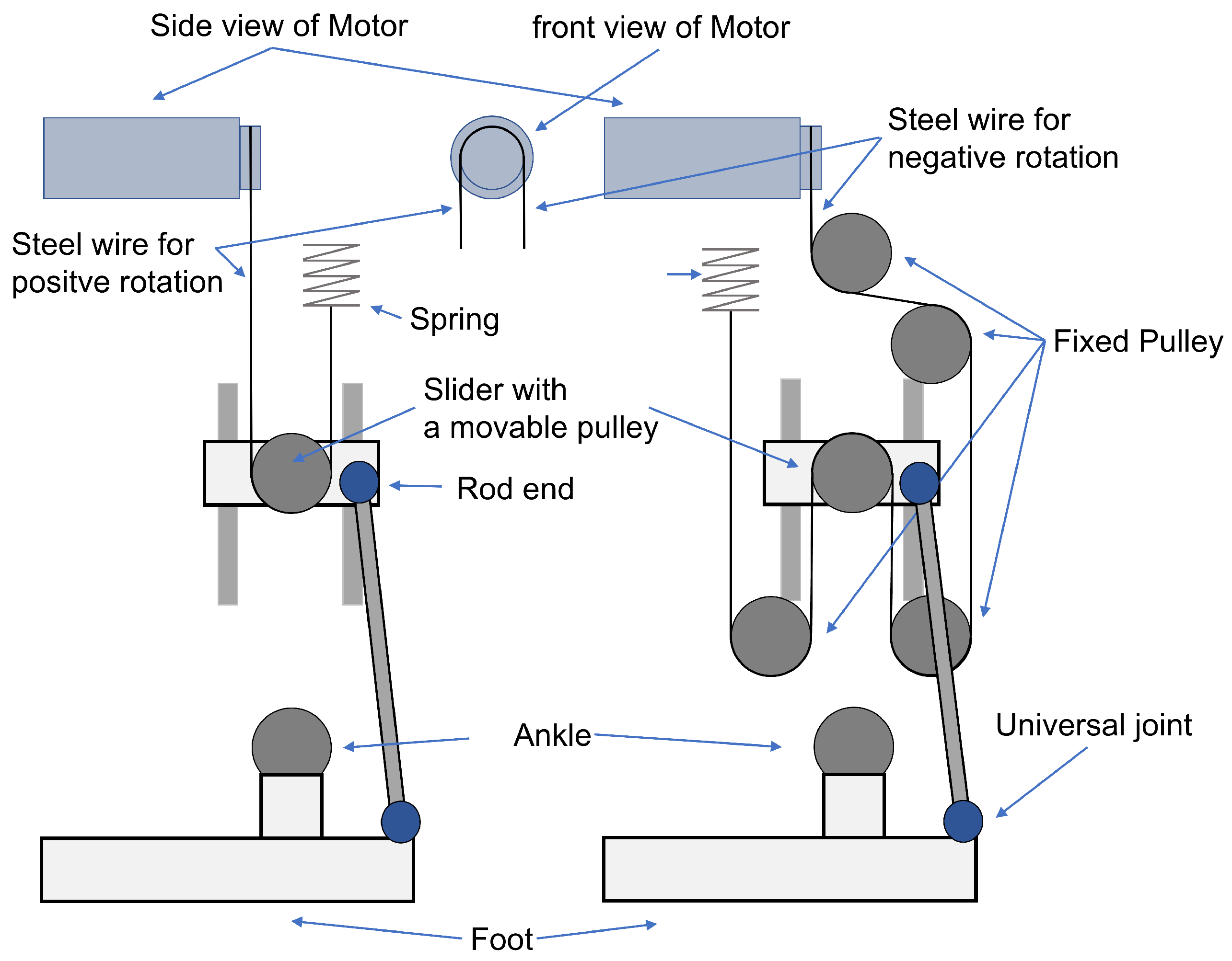
3.3. Ankle
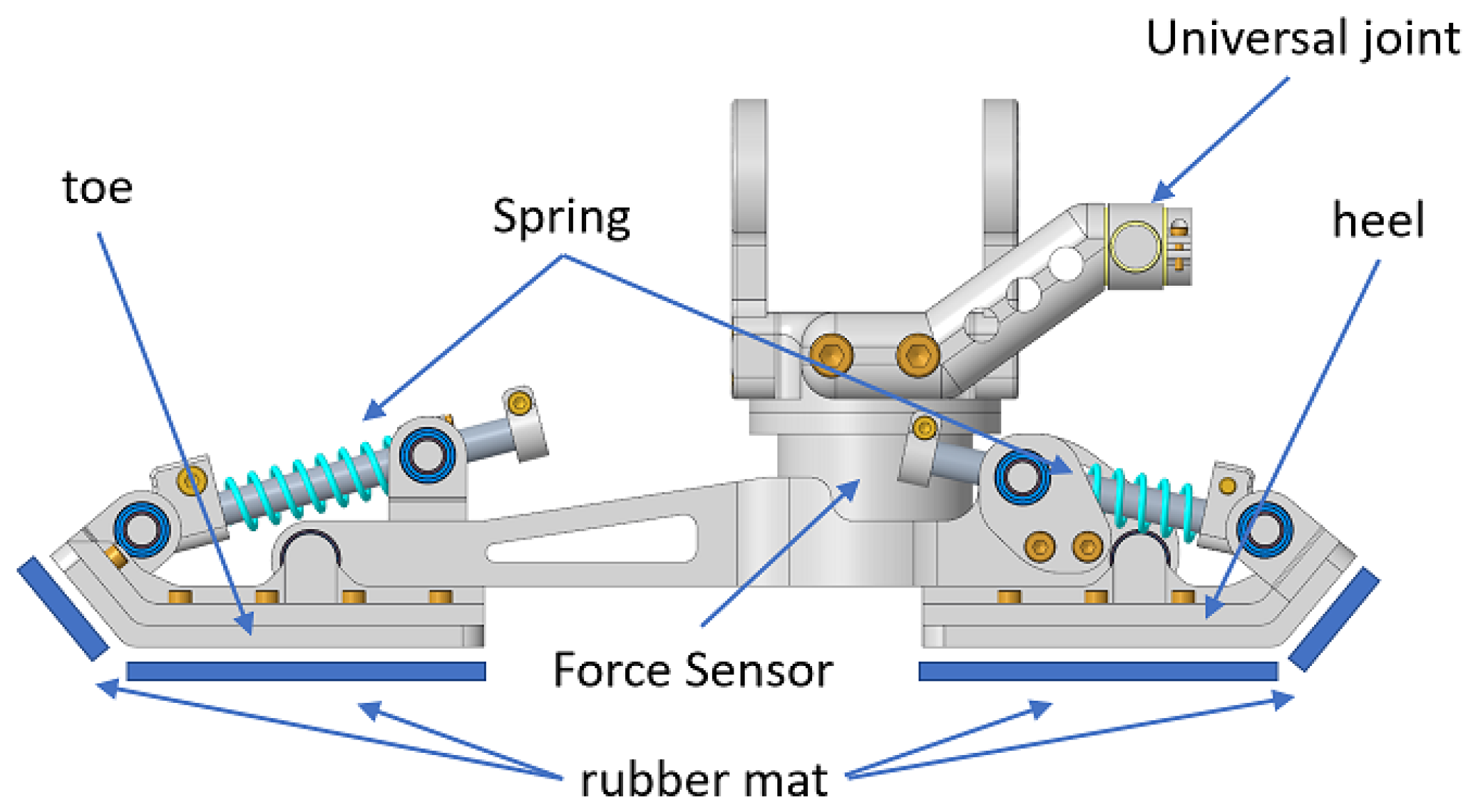
3.4. Foot
4. Kinematic/Dynamic Analysis and Dynamic Model
4.1. Kinematic and Dynamic Parameter of FORREST
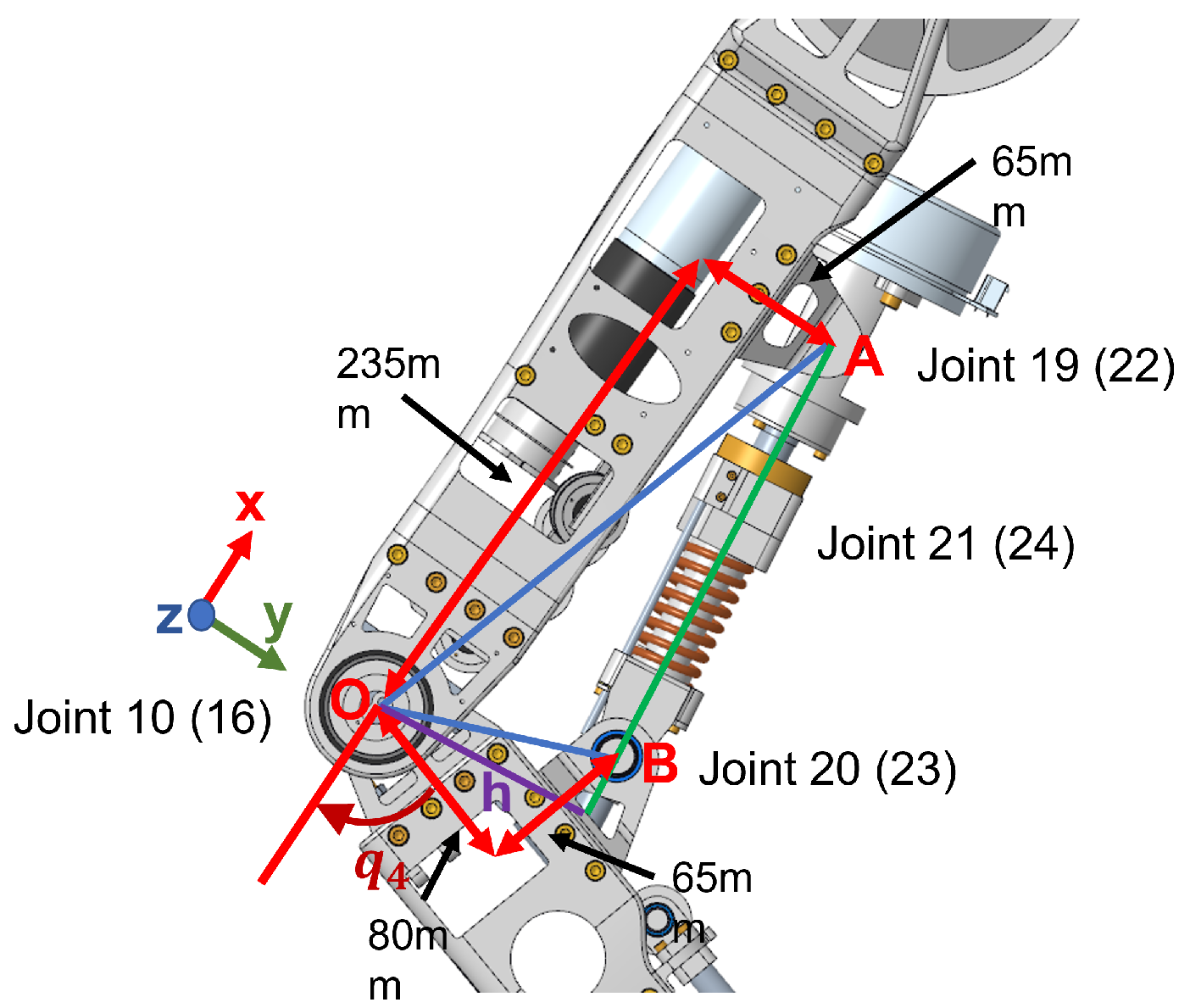
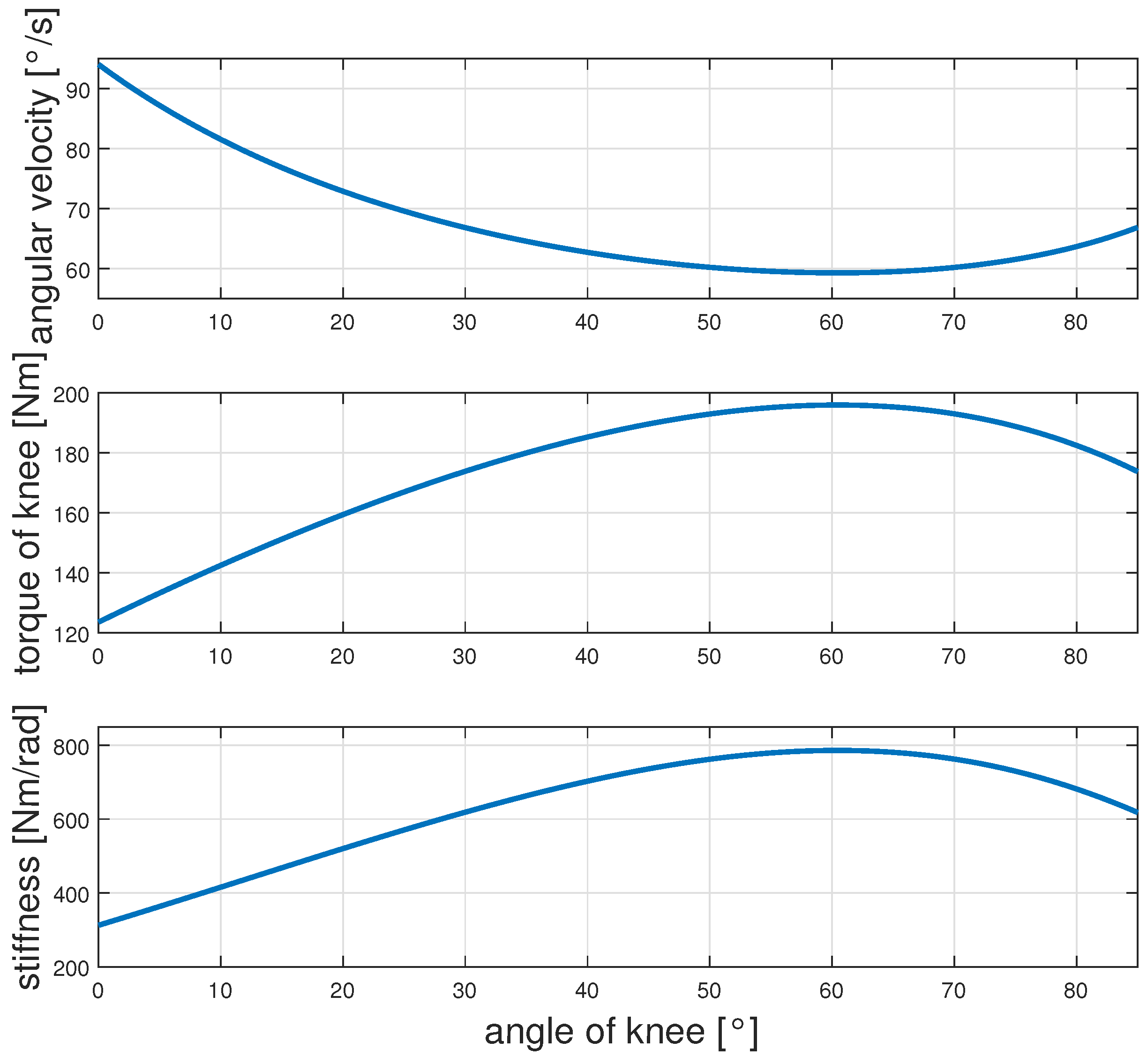
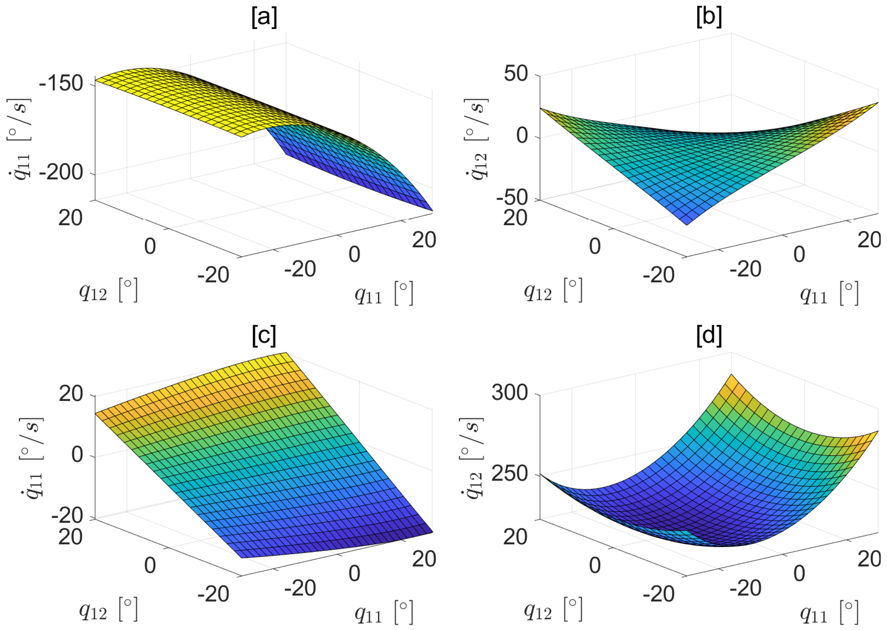
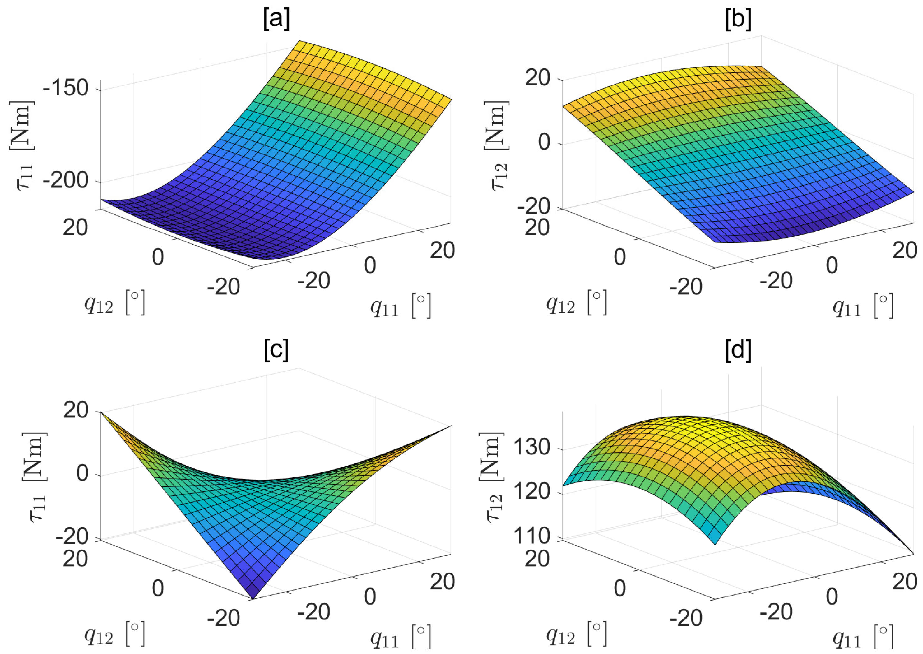
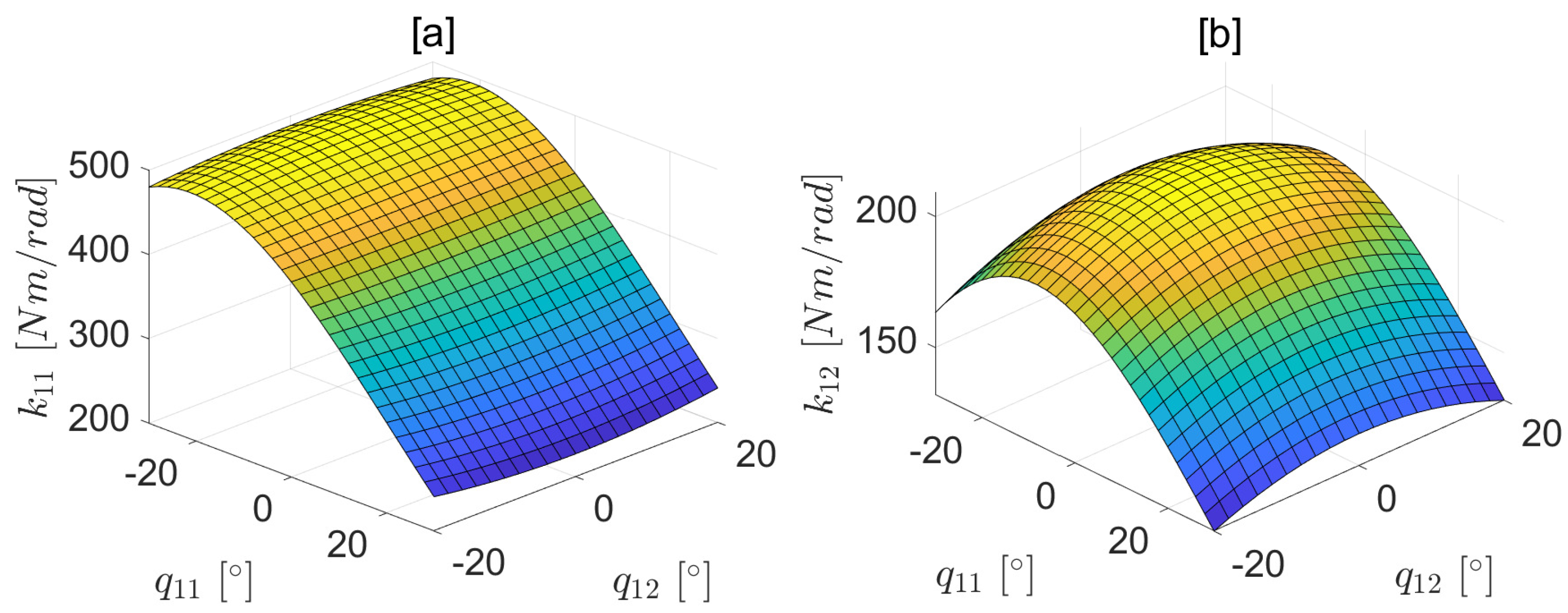
4.2. Knee
4.3. Ankle
4.4. Dynamic Model
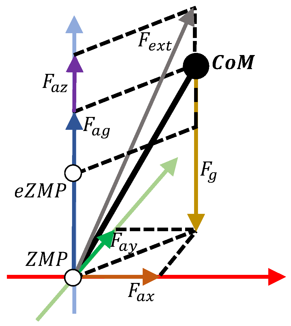
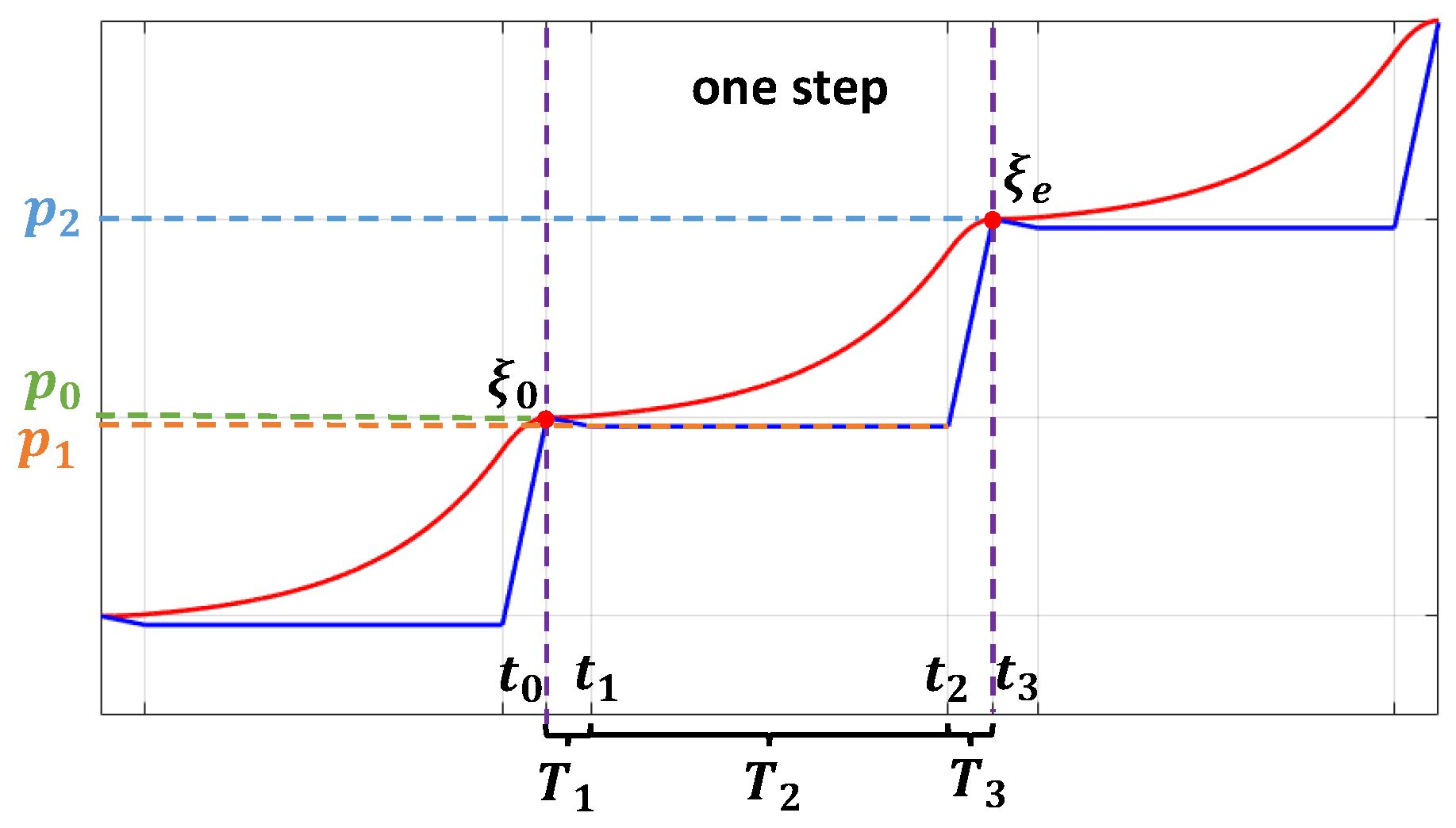
5. Extended CP-Based Walking Pattern Generator
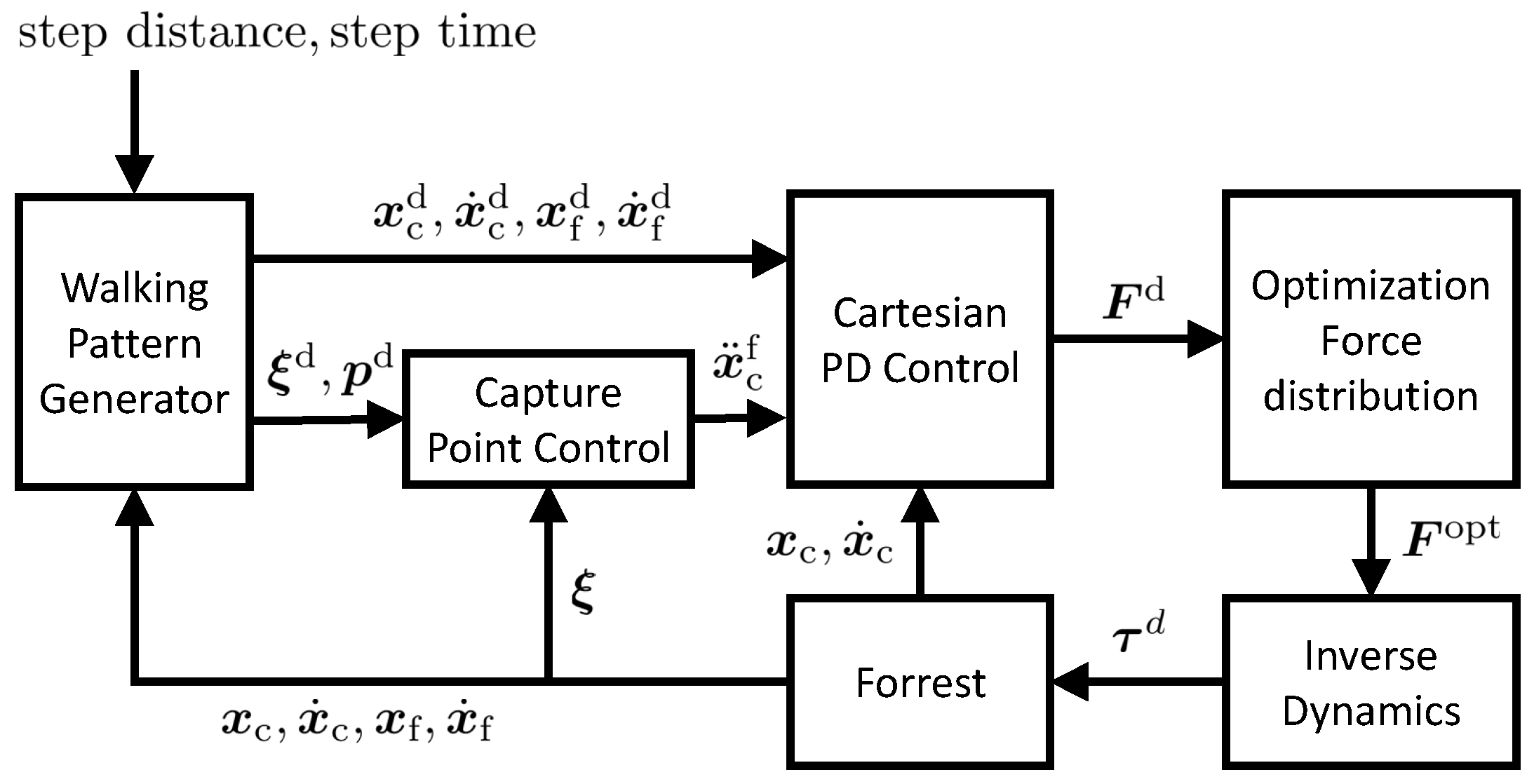
6. Control Strategy
6.1. Capture Point Control
6.2. Cartesian PD Controller
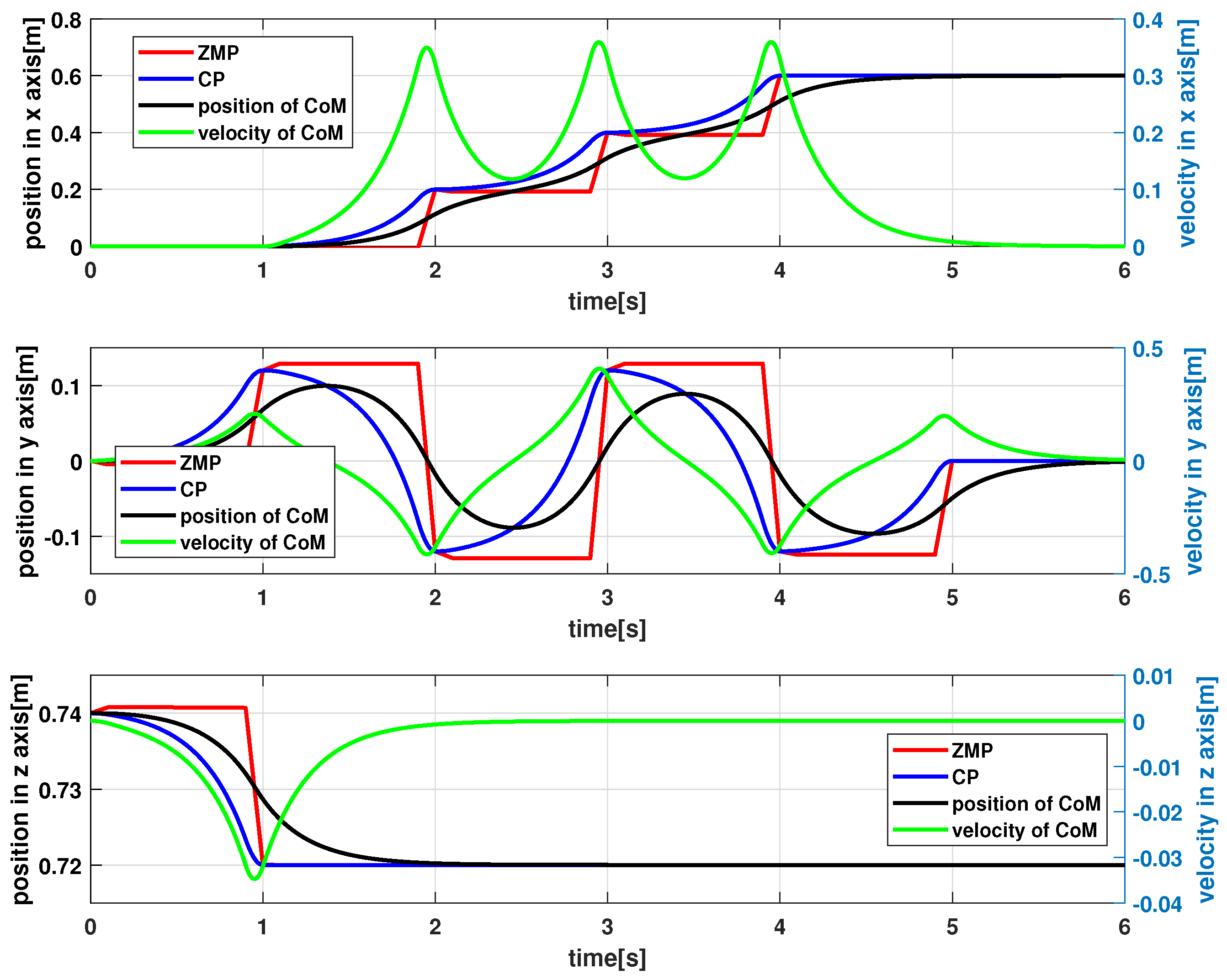
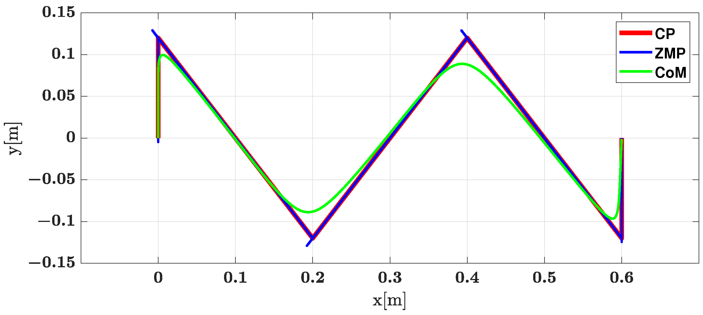
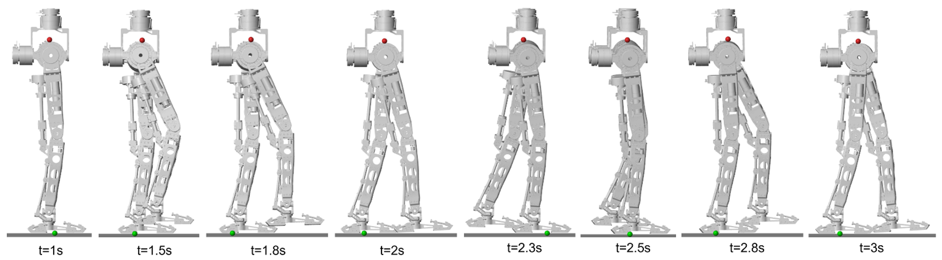
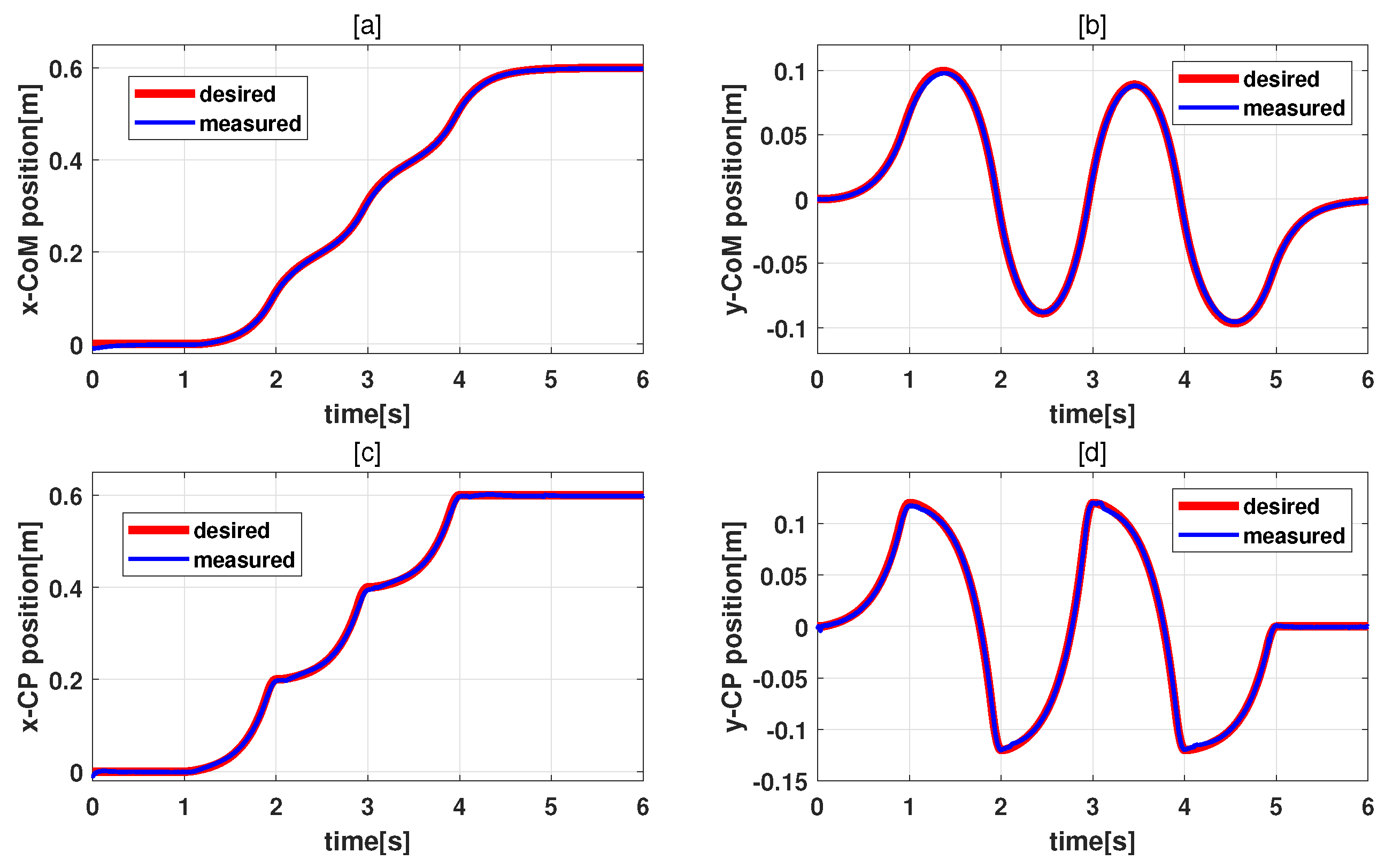
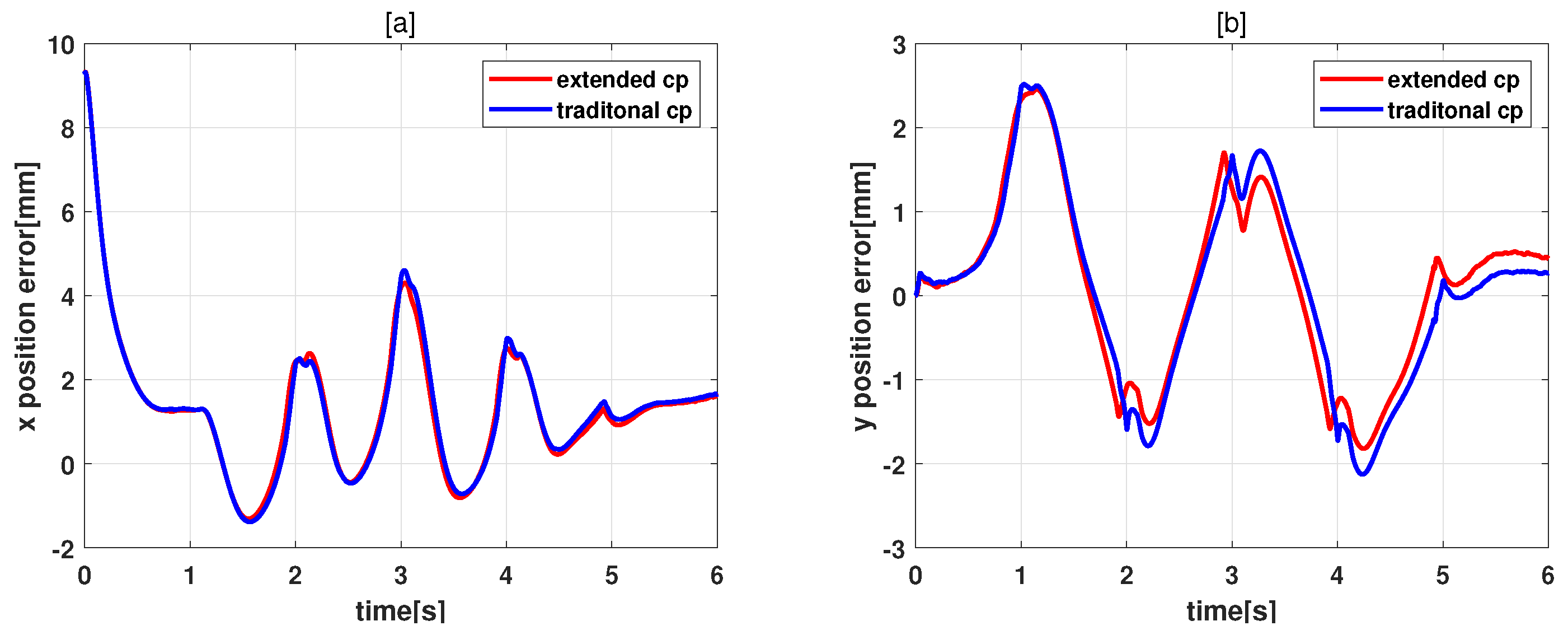
6.3. Results
7. Conclusions
Author Contributions
Funding
Data Availability Statement
Acknowledgments
Conflicts of Interest
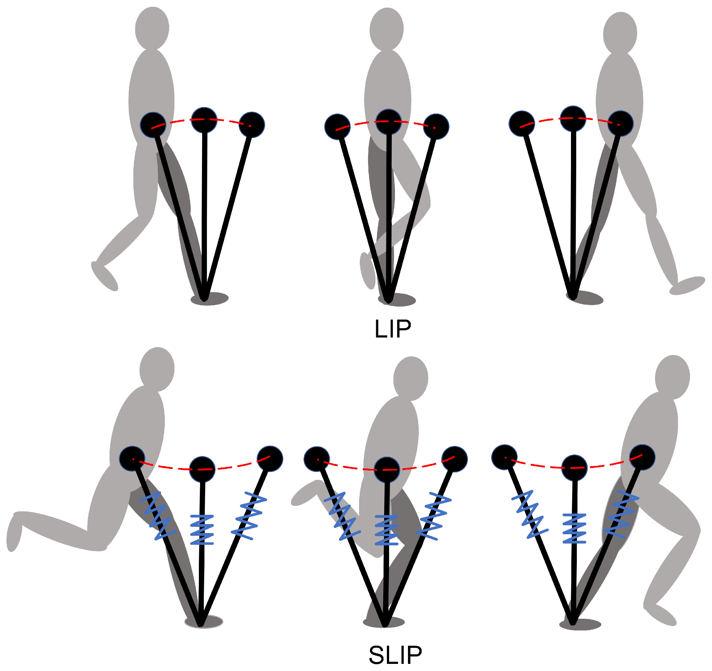
Appendix A. Comparison between the LIP and SLIP Models

References
- Sakagami, Y.; Watanabe, R.; Aoyama, C.; Matsunaga, S.; Higaki, N.; Fujimura, K. The intelligent ASIMO: System overview and integration. In Proceedings of the IEEE/RSJ International Conference on Intelligent Robots and Systems, Lausanne, Switzerland, 30 September–4 October 2002; Volume 3, pp. 2478–2483. [Google Scholar] [CrossRef]
- Hirukawa, H.; Kanehiro, F.; Kaneko, K.; Kajita, S.; Fujiwara, K.; Kawai, Y.; Tomita, F.; Hirai, S.; Tanie, K.; Isozumi, T.; et al. Humanoid robotics platforms developed in HRP. Robot. Auton. Syst. 2004, 48, 165–175. [Google Scholar] [CrossRef]
- Kaneko, K.; Kanehiro, F.; Kajita, S.; Hirukawa, H.; Kawasaki, T.; Hirata, M.; Akachi, K.; Isozumi, T. Humanoid robot HRP-2. In Proceedings of the IEEE International Conference on Robotics and Automation, ICRA’04, New Orleans, LA, USA, 26 April–1 May 2004; Volume 2, pp. 1083–1090. [Google Scholar] [CrossRef]
- Kaneko, K.; Harada, K.; Kanehiro, F.; Miyamori, G.; Akachi, K. Humanoid robot HRP-3. In Proceedings of the 2008 IEEE/RSJ International Conference on Intelligent Robots and Systems, Nice, France, 22–26 September 2008; pp. 2471–2478. [Google Scholar] [CrossRef]
- Kaneko, K.; Kanehiro, F.; Morisawa, M.; Akachi, K.; Miyamori, G.; Hayashi, A.; Kanehira, N. Humanoid robot HRP-4—Humanoid robotics platform with lightweight and slim body. In Proceedings of the 2011 IEEE/RSJ International Conference on Intelligent Robots and Systems, San Francisco, CA, USA, 25–30 September 2011; pp. 4400–4407. [Google Scholar] [CrossRef]
- Kaneko, K.; Kaminaga, H.; Sakaguchi, T.; Kajita, S.; Morisawa, M.; Kumagai, I.; Kanehiro, F. Humanoid Robot HRP-5P: An Electrically Actuated Humanoid Robot with High-Power and Wide-Range Joints. IEEE Robot. Autom. Lett. 2019, 4, 1431–1438. [Google Scholar] [CrossRef]
- Toyota Global Newsroom. Toyota Unveils Third Generation Humanoid Robot T-HR3. November 2017. Available online: https://newsroom.toyota.co.jp/en/download/20110424 (accessed on 31 December 2022).
- WABIAN-2R Biped Robot. Available online: http://www.takanishi.mech.waseda.ac.jp/top/research/wabian/ (accessed on 31 December 2022).
- Englsberger, J.; Werner, A.; Ott, C.; Henze, B.; Roa, M.A.; Garofalo, G.; Burger, R.; Beyer, A.; Eiberger, O.; Schmid, K.; et al. Overview of the torque-controlled humanoid robot TORO. In Proceedings of the 2014 IEEE-RAS International Conference on Humanoid Robots, Madrid, Spain, 18–20 November 2014; pp. 916–923. [Google Scholar] [CrossRef] [Green Version]
- Ott, C.; Baumgärtner, C.; Mayr, J.; Fuchs, M.; Burger, R.; Lee, D.; Eiberger, O.; Albu-Schäffer, A.; Grebenstein, M.; Hirzinger, G. Development of a biped robot with torque controlled joints. In Proceedings of the 2010 10th IEEE-RAS International Conference on Humanoid Robots, Nashville, TN, USA, 6–8 December 2010; pp. 167–173. [Google Scholar] [CrossRef]
- Lohmeier, S.; Loffler, K.; Gienger, M.; Ulbrich, H.; Pfeiffer, F. Computer system and control of biped “Johnnie”. In Proceedings of the IEEE International Conference on Robotics and Automation, ICRA’04, New Orleans, LA, USA, 26 April–1 May 2004; Volume 4, pp. 4222–4227. [Google Scholar] [CrossRef]
- Lohmeier, S. Design and Realization of a Humanoid Robot for Fast and Autonomous Bipedal Locomotion. Ph.D. Thesis, Technische Universität München, Munich, Germany, 2010. [Google Scholar]
- Reher, J.; Ma, W.L.; Ames, A.D. Dynamic walking with compliance on a cassie bipedal robot. In Proceedings of the 2019 18th European Control Conference (ECC), Naples, Italy, 25–28 June 2019. [Google Scholar]
- PAL Biped Robot Reem. 2013. Available online: https://pal-robotics.com/robots/reem-c/ (accessed on 31 December 2022).
- PAL Biped Robot Talos. 2017. Available online: https://pal-robotics.com/robots/talos/ (accessed on 31 December 2022).
- Roig, A.; Kothakota, S.K.; Miguel, N.; Fernbach, P.; Hoffman, E.M.; Marchionni, L. On the hardware design and control architecture of the humanoid robot kangaroo. In Proceedings of the 6th Workshop on Legged Robots during the International Conference on Robotics and Automation (ICRA 2022), Philadelphia, PA, USA, 27 May 2022. [Google Scholar]
- Tesla Biped Robot Optimus. 2022. Available online: https://spectrum.ieee.org/robotics-experts-tesla-bot-optimus (accessed on 31 December 2022).
- Feng, S.; Xinjilefu, X.; Atkeson, C.G.; Kim, J. Optimization based controller design and implementation for the atlas robot in the darpa robotics challenge finals. In Proceedings of the 2015 IEEE-RAS 15th International Conference on Humanoid Robots (Humanoids), Seoul, Republic of Korea, 3–5 November 2015. [Google Scholar]
- Hyon, S.H.; Suewaka, D.; Torii, Y.; Oku, N. Design and experimental evaluation of a fast torque-controlled hydraulic humanoid robot. IEEE/ASME Trans. Mechatron. 2016, 22, 623–634. [Google Scholar] [CrossRef]
- Ugurlu, B.; Tsagarakis, N.G.; Spyrakos-Papastavridis, E.; Caldwell, D.G. Compliant joint modification and real-time dynamic walking implementation on bipedal robot cCub. In Proceedings of the 2011 IEEE International Conference on Mechatronics, Istanbul, Turkey, 13–15 April 2011. [Google Scholar]
- Negrello, F.; Garabini, M.; Catalano, M.G.; Malzahn, J.; Caldwell, D.G.; Bicchi, A.; Tsagarakis, N.G. A modular compliant actuator for emerging high performance and fall-resilient humanoids. In Proceedings of the 2015 IEEE-RAS 15th International Conference on Humanoid Robots (Humanoids), Seoul, Republic of Korea, 3–5 November 2015. [Google Scholar]
- Farley, C.T.; Gonzalez, O. Leg stiffness and stride frequency in human running. J. Biomech. 1996, 29, 181–186. [Google Scholar] [CrossRef] [PubMed]
- Wolf, S.; Eiberger, O.; Hirzinger, G. The DLR FSJ: Energy based design of a variable stiffness joint. In Proceedings of the 2011 IEEE international conference on robotics and automation, Shanghai, China, 9–13 May 2011. [Google Scholar]
- Radford, N.A.; Strawser, P.; Hambuchen, K.; Mehling, J.S.; Verdeyen, W.K.; Donnan, A.S.; Holley, J.; Sanchez, J.; Nguyen, V.; Bridgwater, L.; et al. Valkyrie: Nasa’s first bipedal humanoid robot. J. Field Robot. 2015, 32, 397–419. [Google Scholar] [CrossRef]
- Grizzle, J.W.; Hurst, J.; Morris, B.; Park, H.W.; Sreenath, K. MABEL, a new robotic bipedal walker and runner. In Proceedings of the 2009 American Control Conference, St. Louis, MO, USA, 10–12 June 2009. [Google Scholar]
- Radkhah, K.; Lens, T.; von Stryk, O. Detailed dynamics modeling of BioBiped’s monoarticular and biarticular tendon-driven actuation system. In Proceedings of the 2012 IEEE/RSJ International Conference on Intelligent Robots and Systems, Vilamoura-Algarve, Portugal, 7–12 October 2012. [Google Scholar]
- Loeffl, F.; Werner, A.; Lakatos, D.; Reinecke, J.; Wolf, S.; Burger, R.; Gumpert, T.; Schmidt, F.; Ott, C.; Grebenstein, M.; et al. The dlr c-runner: Concept, design and experiments. In Proceedings of the 2016 IEEE-RAS 16th International Conference on Humanoid Robots (Humanoids), Cancun, Mexico, 15–17 November 2016. [Google Scholar]
- Kajita, S.; Kanehiro, F.; Kaneko, K.; Yokoi, K.; Hirukawa, H. The 3D linear inverted pendulum mode: A simple modeling for a biped walking pattern generation. In Proceedings of the 2001 IEEE/RSJ International Conference on Intelligent Robots and Systems. Expanding the Societal Role of Robotics in the the Next Millennium (Cat. No. 01CH37180), Maui, HI, USA, 29 October–3 November 2001; Volume 1. [Google Scholar]
- Kajita, S.; Kanehiro, F.; Kaneko, K.; Fujiwara, K.; Harada, K.; Yokoi, K.; Hirukawa, H. Biped walking pattern generation by using preview control of zero-moment point. In Proceedings of the 2003 IEEE international conference on robotics and automation (Cat. No. 03CH37422), Taipei, Taiwan, 14–19 September 2003; Volume 2. [Google Scholar]
- Park, I.-W.; Kim, J.-Y.; Oh, J.-H. Online biped walking pattern generation for humanoid robot khr-3(kaist humanoid robot-3: Hubo). In Proceedings of the 2006 6th IEEE-RAS International Conference on Humanoid Robots, Genova, Italy, 4–6 December 2006; pp. 398–403. [Google Scholar]
- Takenaka, T.; Matsumoto, T.; Yoshiike, T. Real time motion generation and control for biped robot-1st report: Walking gait pattern generation. In Proceedings of the 2009 IEEE/RSJ International Conference on Intelligent Robots and Systems, St. Louis, MO, USA, 10–15 October 2009. [Google Scholar]
- Takenaka, T.; Matsumoto, T.; Yoshiike, T.; Shirokura, S. Real time motion generation and control for biped robot-2nd report: Running gait pattern generation. In Proceedings of the 2009 IEEE/RSJ International Conference on Intelligent Robots and Systems, St. Louis, MO, USA, 10–15 October 2009. [Google Scholar]
- Takenaka, T.; Matsumoto, T.; Yoshiike, T. Real time motion generation and control for biped robot-3rd report: Dynamics error compensation. In Proceedings of the 2009 IEEE/RSJ International Conference on Intelligent Robots and Systems, St. Louis, MO, USA, 10–15 October 2009. [Google Scholar]
- Englsberger, J.; Ott, C.; Roa, M.A.; Albu-Schäffer, A.; Hirzinger, G. Bipedal walking control based on capture point dynamics. In Proceedings of the 2011 IEEE/RSJ International Conference on Intelligent Robots and Systems, St. Louis, MO, USA, 10–15 October 2011. [Google Scholar]
- Englsberger, J.; Ott, C.; Albu-Schäffer, A. Three-dimensional bipedal walking control using divergent component of motion. In Proceedings of the 2013 IEEE/RSJ International Conference on Intelligent Robots and Systems, Tokyo, Japan, 3–7 November 2013; pp. 2600–2607. [Google Scholar]
- Hopkins, M.A.; Hong, D.W.; Leonessa, A. Humanoid locomotion on uneven terrain using the time-varying divergent component of motion. In Proceedings of the 2014 IEEE-RAS International Conference on Humanoid Robots, Madrid, Spain, 18–20 November 2014; pp. 266–272. [Google Scholar]
- Kajita, S.; Benallegue, M.; Cisneros, R.; Sakaguchi, T.; Nakaoka, S.; Morisawa, M.; Kaneko, K.; Kanehiro, F. Biped walking pattern generation based on spatially quantized dynamics. In Proceedings of the 2017 IEEE-RAS 17th International Conference on Humanoid Robotics (Humanoids), Birmingham, UK, 15–17 November 2017; pp. 599–605. [Google Scholar]
- Caron, S.; Escande, A.; Lanari, L.; Mallein, B. Capturability based pattern generation for walking with variable height. IEEE Trans. Robot. 2020, 36, 517–536. [Google Scholar] [CrossRef] [Green Version]
- Tazaki, Y.; Hanasaki, S.; Yukizaki, S.; Mitazono, Y.; Nagano, H.; Yokokohji, Y. A continuous-time walking pattern generator for realizing seamless transition between flat-contact and heel-to-toe walking. Adv. Robot. 2023, 37, 316–328. [Google Scholar] [CrossRef]
- Geyer, H.; Seyfarth, A.; Blickhan, R. Spring-mass running: Simple approximate solution and application to gait stability. J. Theor. Biol. 2005, 232, 315–328. [Google Scholar] [CrossRef] [PubMed] [Green Version]
- Wensing, P.M.; Orin, D.E. High-speed humanoid running through control with a 3D-SLIP model. In Proceedings of the 2013 IEEE/RSJ International Conference on Intelligent Robots and Systems, Tokyo, Japan, 3–7 November 2013. [Google Scholar]
- Kuo, C.-Y.; Shin, H.; Kamioka, T.; Matsubara, T. TDE2-MBRL: Energy-exchange Dynamics Learning with Task Decomposition for Spring-loaded Bipedal Robot Locomotion. In Proceedings of the 2022 IEEE-RAS 21st International Conference on Humanoid Robots (Humanoids), Ginowan, Japan, 28–30 November 2022; pp. 550–557. [Google Scholar] [CrossRef]
- Takenaka, T.; Matsumoto, T.; Yoshiike, T.; Hasegawa, T.; Shirokura, S.; Kaneko, H.; Orita, A. Real time motion generation and control for biped robot-4th report: Integrated balance control. In Proceedings of the 2009 IEEE/RSJ International Conference on Intelligent Robots and Systems, St. Louis, MO, USA, 10–15 October 2009. [Google Scholar]
- Henze, B.; Dietrich, A.; Ott, C. An approach to combine balancing with hierarchical whole-body control for legged humanoid robots. IEEE Robot. Autom. Lett. 2015, 1, 700–707. [Google Scholar] [CrossRef]
- Henze, B.; Roa, M.A.; Ott, C. Passivity-based whole-body balancing for torque-controlled humanoid robots in multi-contact scenarios. Int. J. Robot. Res. 2016, 35, 1522–1543. [Google Scholar] [CrossRef]
- Mesesan, G.; Englsberger, J.; Henze, B.; Ott, C. Dynamic multi-contact transitions for humanoid robots using divergent component of motion. In Proceedings of the 2017 IEEE International Conference on Robotics and Automation (ICRA), Singapore, 29 May–3 June 2017. [Google Scholar]
- Henze, B.; Balachandran, R.; Roa-Garzon, M.A.; Ott, C.; Albu-Schäffer, A. Passivity analysis and control of humanoid robots on movable ground. IEEE Robot. Autom. Lett. 2018, 3, 3457–3464. [Google Scholar] [CrossRef]
- Ding, J.; Xiao, X. Two-stage optimization for energy-efficient bipedal walking. J. Mech. Sci. Technol. 2020, 34, 3833–3844. [Google Scholar] [CrossRef]
- Liu, C.; Zhang, T.; Liu, M.; Chen, Q. Active balance control of humanoid locomotion based on foot position compensation. J. Bionic Eng. 2020, 17, 134–147. [Google Scholar] [CrossRef]
- Reher, J.P.; Hereid, A.; Kolathaya, S.; Hubicki, C.M.; Ames, A.D. Algorithmic foundations of realizing multi-contact locomotion on the humanoid robot DURUS. In Algorithmic Foundations of Robotics XII: Proceedings of the Twelfth Workshop on the Algorithmic Foundations of Robotics; Springer International Publishing: Cham, Switzerland, 2020. [Google Scholar]
- Orozco-Soto, S.M.; Ibarra-Zannatha, J.M.; Kheddar, A. Gait Synthesis and Biped Locomotion Control of the HRP-4 Humanoid. In Proceedings of the 2021 XXIII Robotics Mexican Congress (ComRob), Tijuana, Mexico, 27–29 October 2021. [Google Scholar]
- Daneshmand, E.; Khadiv, M.; Grimminger, F.; Righetti, L. Variable horizon mpc with swing foot dynamics for bipedal walking control. IEEE Robot. Autom. Lett. 2021, 6, 2349–2356. [Google Scholar] [CrossRef]
- García, G.; Griffin, R.; Pratt, J. MPC-based locomotion control of bipedal robots with line-feet contact using centroidal dynamics. In Proceedings of the 2020 IEEE-RAS 20th International Conference on Humanoid Robots (Humanoids), Munich, Germany, 19–21 July 2021. [Google Scholar]
- Galliker, M.Y.; Csomay-Shanklin, N.; Grandia, R.; Taylor, A.J.; Farshidian, F.; Hutter, M.; Ames, A.D. Planar Bipedal Locomotion with Nonlinear Model Predictive Control: Online Gait Generation using Whole-Body Dynamics. In Proceedings of the 2022 IEEE-RAS 21st International Conference on Humanoid Robots (Humanoids), Ginowan, Japan, 28–30 November 2022. [Google Scholar]
- Villa, N.A.; Fernbach, P.; Naveau, M.; Saurel, G.; Dantec, E.; Mansard, N.; Stasse, O. Torque Controlled Locomotion of a Biped Robot with Link Flexibility. In Proceedings of the 2022 IEEE-RAS 21st International Conference on Humanoid Robots (Humanoids), Ginowan, Japan, 28–30 November 2022. [Google Scholar]
- Dantec, E.; Naveau, M.; Fernbach, P.; Villa, N.; Saurel, G.; Stasse, O.; Taïx, M.; Mansard, N. Whole-Body Model Predictive Control for Biped Locomotion on a Torque-Controlled Humanoid Robot. In Proceedings of the 2022 IEEE-RAS 21st International Conference on Humanoid Robots (Humanoids), Ginowan, Japan, 28–30 November 2022. [Google Scholar]
- Ramuzat, N.; Boria, S.; Stasse, O. Passive inverse dynamics control using a global energy tank for torque-controlled humanoid robots in multi-contact. IEEE Robot. Autom. Lett. 2022, 7, 2787–2794. [Google Scholar] [CrossRef]


| Segment | Weight [kg] | Height [mm] |
|---|---|---|
| base | 17.14 | 250 |
| thigh | 5.83 | 405 |
| calf | 2.8 | 405 |
| foot | 0.35 | 105 |
| total | 35.1 | 1165 |
| Joint | Max Toque [Nm] | Max Speed [rpm] |
|---|---|---|
| hip 1 | 120 | 31.9 |
| hip 2 | 107 | 19.9 |
| hip 3 | 315 | 29 |
| knee | 195 | 15.8 |
| ankle 1 | 212 | 35 |
| ankle 2 | 138 | 47 |
| FORREST | Toro | Lola | TALOS | C-Runner | MABEL | BioBiped | |
|---|---|---|---|---|---|---|---|
| balance | ◯ | ◯ | ◯ | ◯ | × | × | × |
| compliance | active + passive | active | active | active | passive | passive | passive |
| Link Id | Child Id | Parent Id | m [kg] | r [m] | [kg m2] | |
|---|---|---|---|---|---|---|
| 1 | 2 | 0 | ||||
| 2 | 3 | 1 | ||||
| 3 | 4 | 2 | ||||
| 4 | 5 | 3 | ||||
| 5 | 6 | 4 | ||||
| 6 | 7, 13 | 5 | ||||
| 7 | 8 | 6 | ||||
| 8 | 9 | 7 | ||||
| 9 | 10 | 8 | ||||
| 10 | 11 | 9 | ||||
| 11 | 12 | 10 | ||||
| 12 | 11 | |||||
| 13 | 14 | 6 | ||||
| 14 | 15 | 13 | ||||
| 15 | 16 | 14 | ||||
| 16 | 17 | 15 | ||||
| 17 | 18 | 16 | ||||
| 18 | 17 |
Disclaimer/Publisher’s Note: The statements, opinions and data contained in all publications are solely those of the individual author(s) and contributor(s) and not of MDPI and/or the editor(s). MDPI and/or the editor(s) disclaim responsibility for any injury to people or property resulting from any ideas, methods, instructions or products referred to in the content. |
© 2023 by the authors. Licensee MDPI, Basel, Switzerland. This article is an open access article distributed under the terms and conditions of the Creative Commons Attribution (CC BY) license (https://creativecommons.org/licenses/by/4.0/).
Share and Cite
Zhu, H.; Thomas, U. Mechanical Design of a Biped Robot FORREST and an Extended Capture-Point-Based Walking Pattern Generator. Robotics 2023, 12, 82. https://doi.org/10.3390/robotics12030082
Zhu H, Thomas U. Mechanical Design of a Biped Robot FORREST and an Extended Capture-Point-Based Walking Pattern Generator. Robotics. 2023; 12(3):82. https://doi.org/10.3390/robotics12030082
Chicago/Turabian StyleZhu, Hongxi, and Ulrike Thomas. 2023. "Mechanical Design of a Biped Robot FORREST and an Extended Capture-Point-Based Walking Pattern Generator" Robotics 12, no. 3: 82. https://doi.org/10.3390/robotics12030082