
Experiments on the Artificial Potential Field with Local Attractors for Mobile Robot Navigation

 ,
,  , and
, and 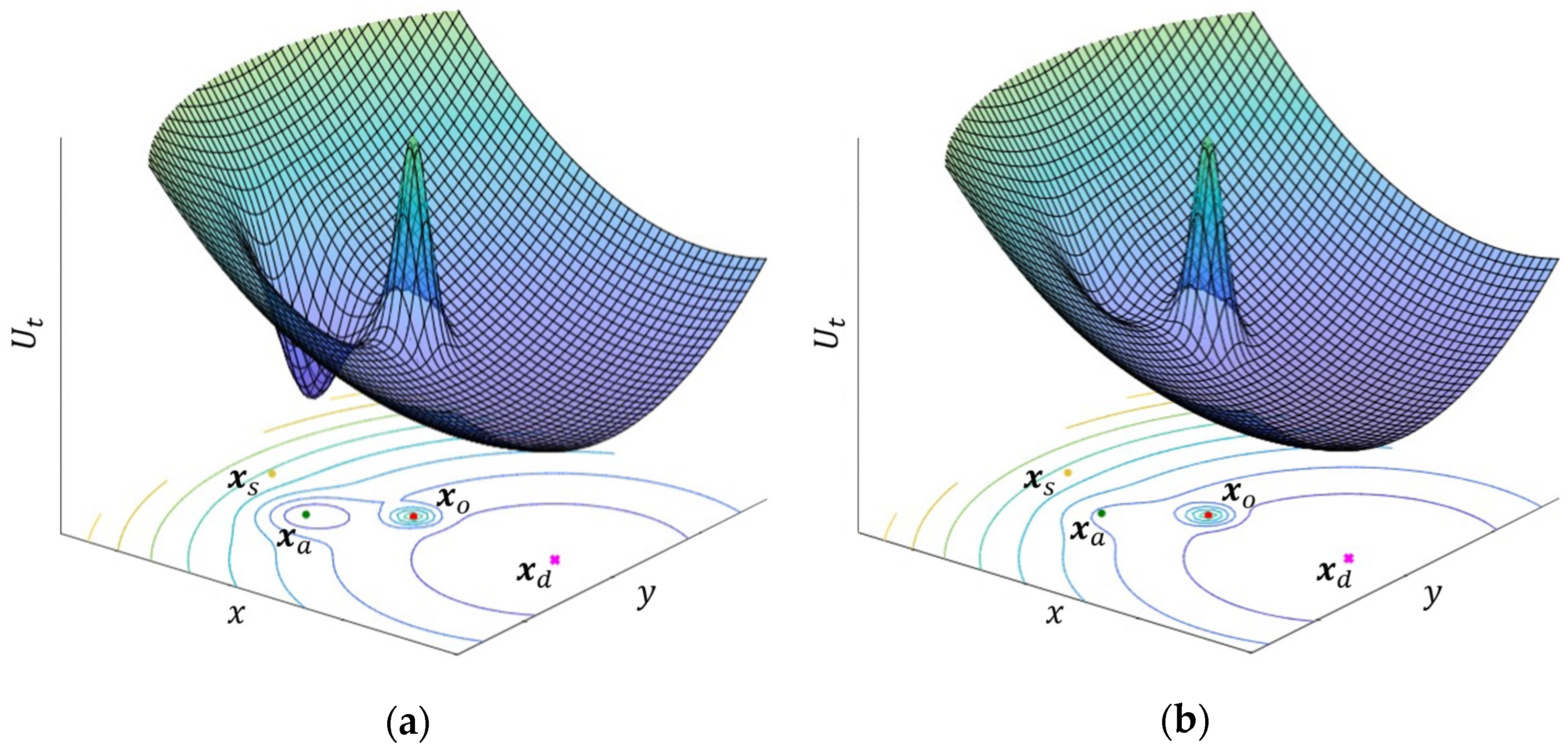
Abstract
:1. Introduction
- validation of the potential field with local attractors through laboratory tests;
- proposal of an essential experimental setup that can run the potential field with local attractors in real-time;
- experimental analysis of the influence of obstacle pose, local attractor intensity, and robot velocity;
- analysis of the strengths and limitations of the proposed method on the base of the experimental results.
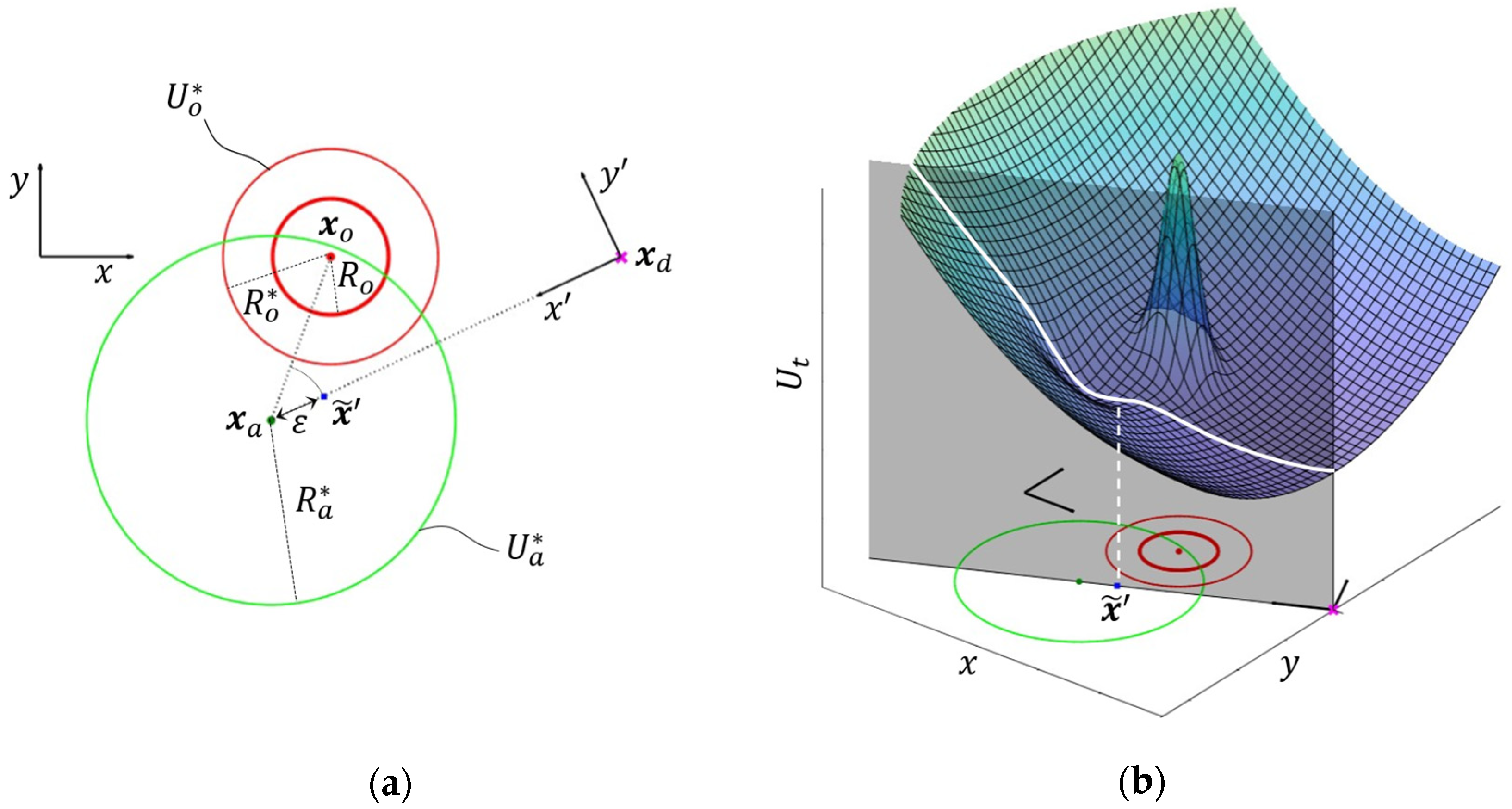
2. Artificial Potential Field with Local Attractors
2.1. Theoretical Formulation
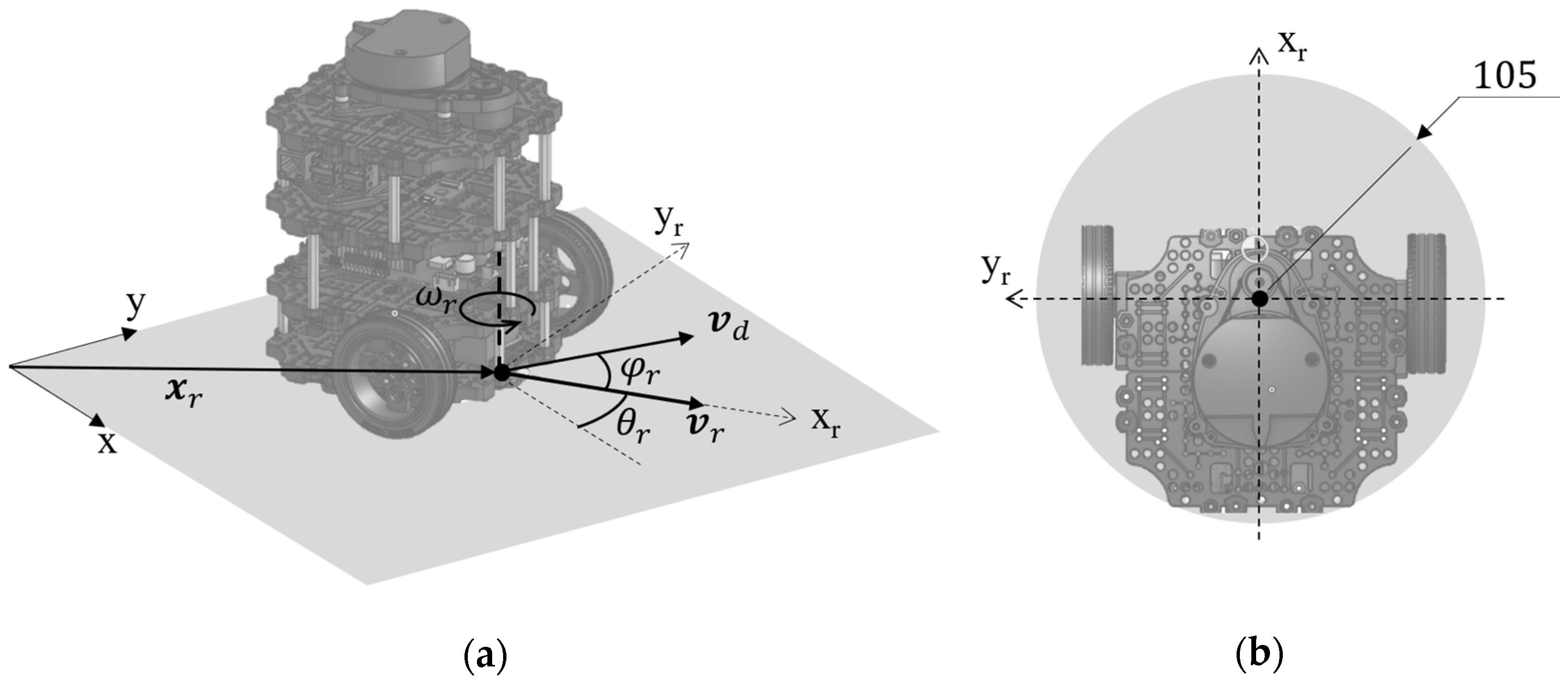
2.2. Application to Mobile Robot
3. Experimental Tests
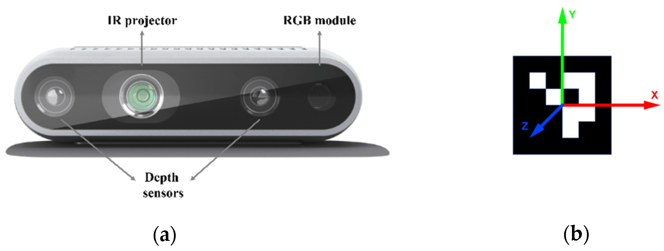
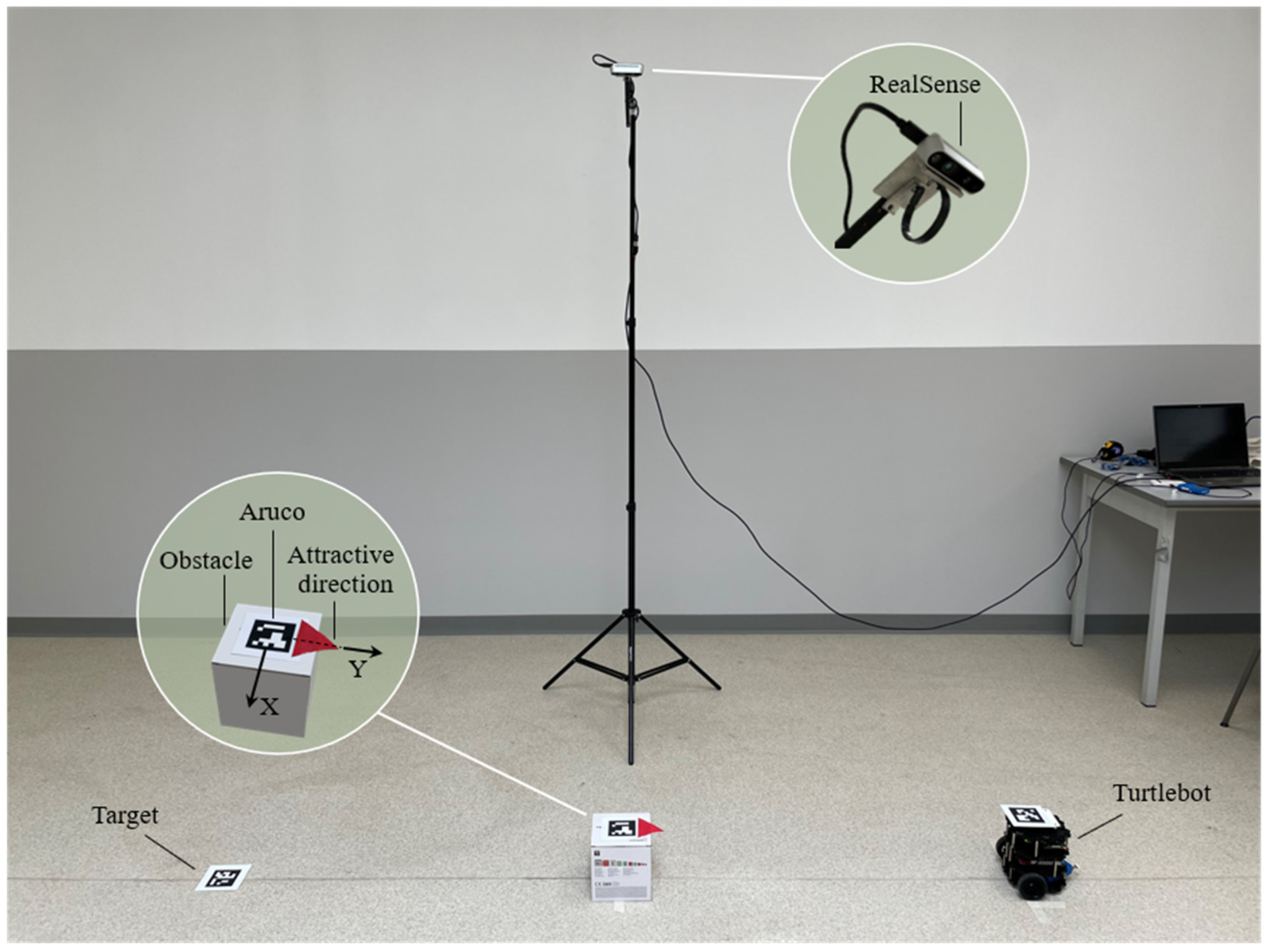
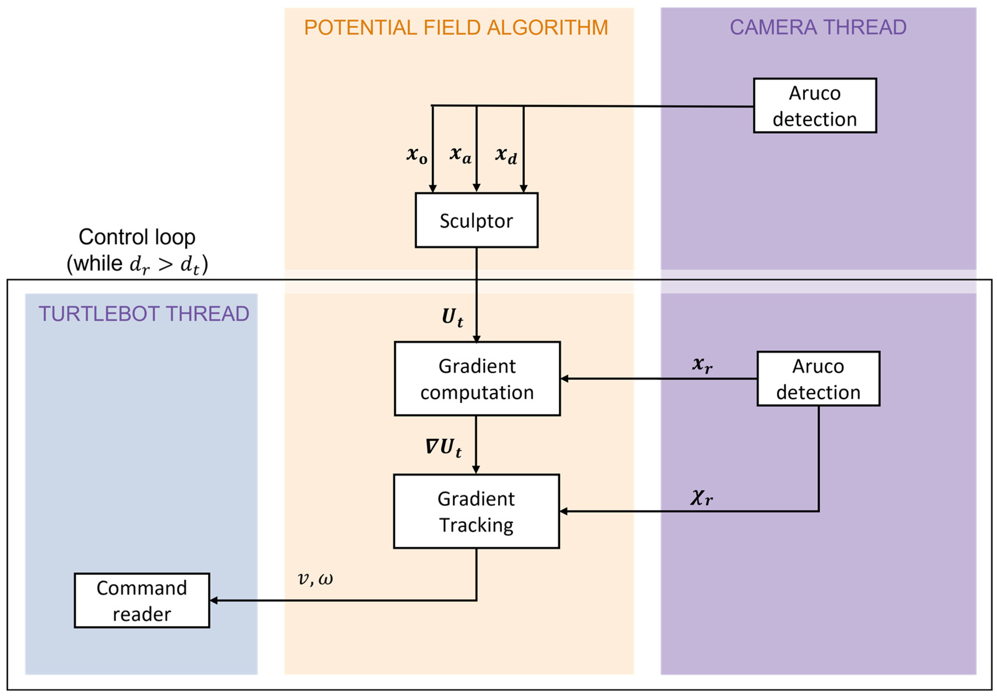
3.1. Laboratory Setup
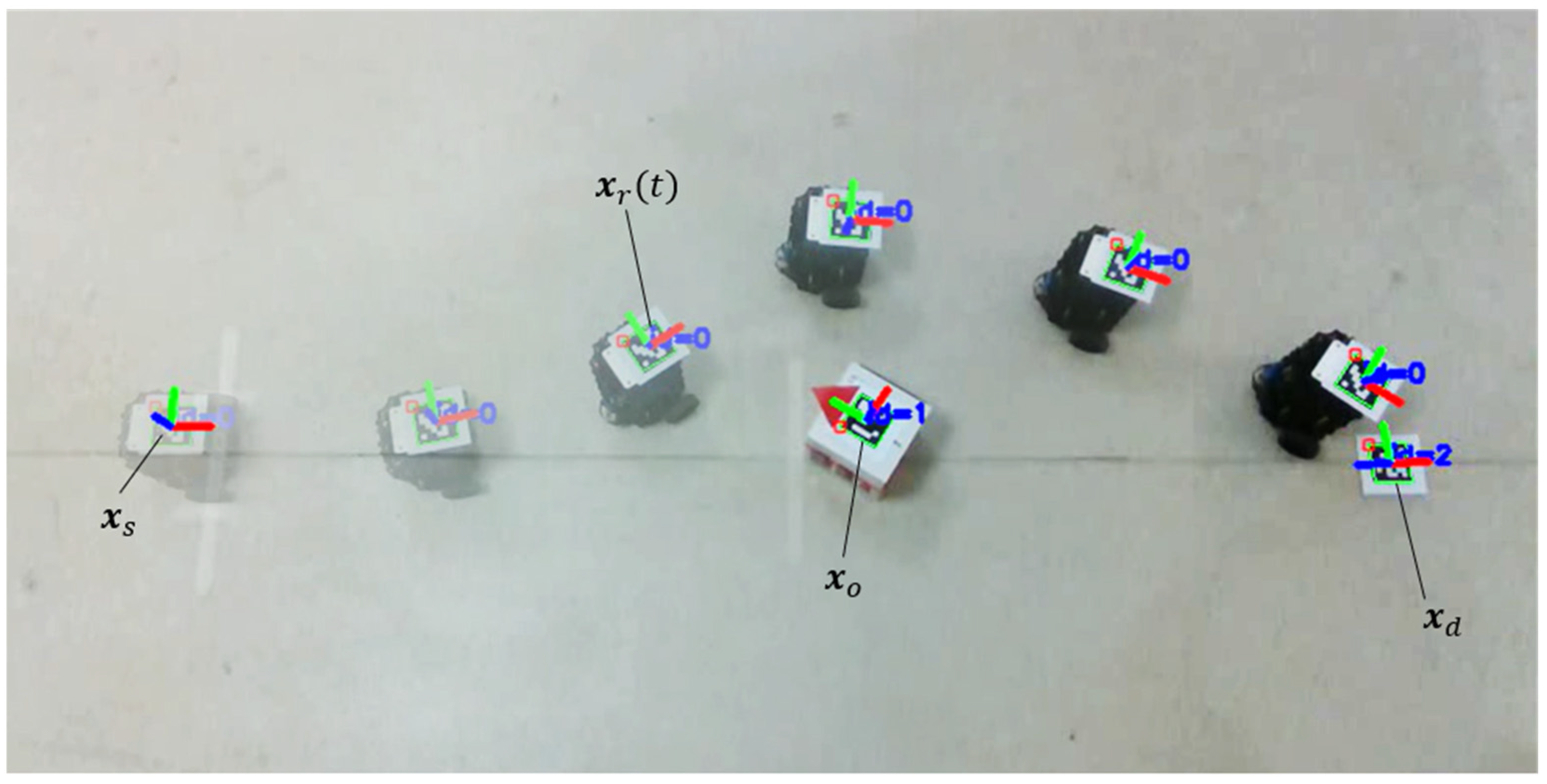
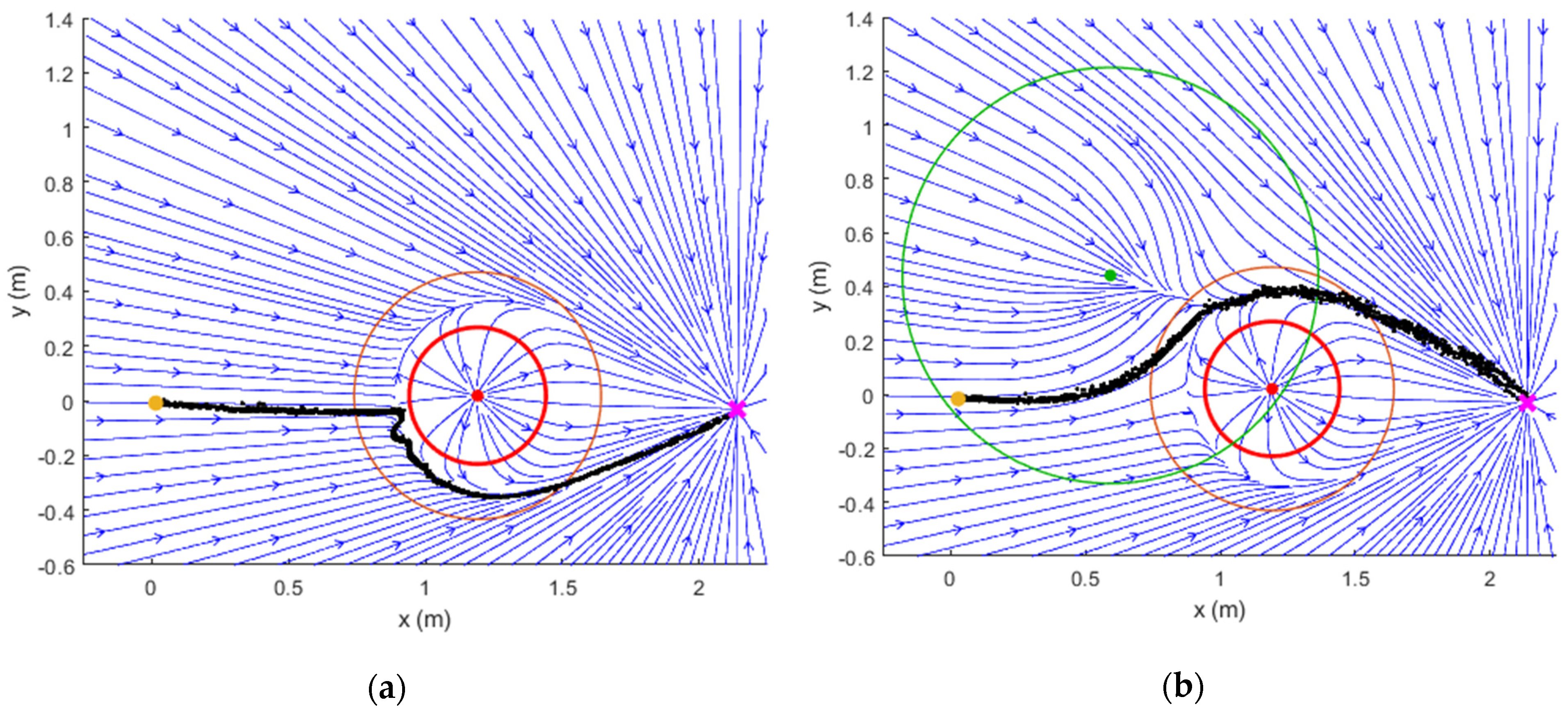
3.2. Results
4. Discussion
4.1. Obstacle Modelling
4.2. Dynamic Environment
4.3. Multiple Agents
4.4. Gradient Tracking
4.5. Attractor Modelling
5. Conclusions
Supplementary Materials
Author Contributions
Funding
Data Availability Statement
Acknowledgments
Conflicts of Interest
References
- Khatib, O. Real-time obstacle avoidance for manipulators and mobile robots. Int. J. Robot. Res. 1986, 5, 90–98. [Google Scholar] [CrossRef]
- Volpe, R.; Khosla, P. Manipulator control with superquadratic artificial potential functions: Theory and experiments. IEEE Trans. Syst. Man. Cybern. 1990, 20, 1423–1436. [Google Scholar] [CrossRef] [Green Version]
- Rimon, E.; Koditschek, D.E. Exact Robot Navigation using Artificial Potential Functions. IEEE Trans. Robot. Autom. 1992, 8, 501–518. [Google Scholar] [CrossRef] [Green Version]
- Vadakkepat, P.; Tan, K.C.; Ming-Liang, W. Evolutionary artificial potential fields and their application in real time robot path planning. In Proceedings of the 2000 Congress on Evolutionary Computation, CEC 2000, La Jolla, CA, USA, 16–19 July 2000; pp. 256–263. [Google Scholar] [CrossRef]
- Paromtchik, I.E.; Nassal, U.M. Reactive Motion Control for an Omnidirectional Mobile Robot. In Proceedings of the Third European Control Conference, Rome, Italy, 5–8 September 1995; pp. 5–8. [Google Scholar]
- Long, Z. Virtual target point-based obstacle-avoidance method for manipulator systems in a cluttered environment. Eng. Optim. 2020, 52, 1957–1973. [Google Scholar] [CrossRef]
- Zou, X.; Zhu, J. Virtual local target method for avoiding local minimum in potential field based robot navigation. J. Zhejiang Univ. Sci. 2003, 4, 264–269. [Google Scholar] [CrossRef]
- Azzabi, A.; Nouri, K. An advanced potential field method proposed for mobile robot path planning. Trans. Inst. Meas. Control 2019, 41, 3132–3144. [Google Scholar] [CrossRef]
- SRostami, M.H.; Sangaiah, A.K.; Wang, J.; Liu, X. Obstacle avoidance of mobile robots using modified artificial potential field algorithm. EURASIP J. Wirel. Commun. Netw. 2019, 2019, 70. [Google Scholar] [CrossRef] [Green Version]
- Jung, J.H.; Kim, D.H. Local path planning of a mobile robot using a novel grid-based potential method. Int. J. Fuzzy Log. Intell. Syst. 2020, 20, 26–34. [Google Scholar] [CrossRef]
- Patle, B.K.; Babu, L.G.; Pandey, A.; Parhi, D.R.K.; Jagadeesh, A. A review: On path planning strategies for navigation of mobile robot. Def. Technol. 2019, 15, 582–606. [Google Scholar] [CrossRef]
- Ge, S.S.; Cui, Y.J. New potential functions for mobile robot path planning. IEEE Trans. Robot. Autom. 2000, 16, 615–620. [Google Scholar] [CrossRef] [Green Version]
- Sfeir, J.; Saad, M.; Saliah-Hassane, H. An improved Artificial Potential Field approach to real-time mobile robot path planning in an unknown environment. In Proceedings of the ROSE 2011-IEEE International Symposium on Robotic and Sensors Environments, Proceedings 2011, Montreal, QC, Canada, 17–18 September 2011; pp. 208–213. [Google Scholar] [CrossRef]
- Duhé, J.F.; Victor, S.; Melchior, P. Contributions on artificial potential field method for effective obstacle avoidance. Fract. Calc. Appl. Anal. 2021, 24, 421–446. [Google Scholar] [CrossRef]
- Scimmi, L.S.; Melchiorre, M.; Troise, M.; Mauro, S.; Pastorelli, S. A Practical and Effective Layout for a Safe Human-Robot Collaborative Assembly Task. Appl. Sci. 2021, 11, 1763. [Google Scholar] [CrossRef]
- Scimmi, L.S.; Melchiorre, M.; Mauro, S.; Pastorelli, S. Experimental Real-Time Setup for Vision Driven Hand-Over with a Collaborative Robot. In Proceedings of the 2019 International Conference on Control, Automation and Diagnosis, ICCAD 2019-Proceedings 2019, Grenoble, France, 2–4 July 2019. [Google Scholar] [CrossRef]
- Melchiorre, M.; Scimmi, L.S.; Mauro, S.; Pastorelli, S. A Novel Constrained Trajectory Planner for Safe Human-robot Collaboration. In Proceedings of the ICINCO 2022, Lisbon, Portugal, 14–16 July 2022. [Google Scholar] [CrossRef]
- Güldner, J.; Utkin, V.I. Tracking the gradient of artificial potential fields: Sliding mode control for mobile robots. Int. J. Control 1996, 63, 417–432. [Google Scholar] [CrossRef]
- De Medio, C.; Oriolo, G. Robot Obstacle Avoidance Using Vortex Fields. In Advances in Robot Kinematics; Springer: Berlin/Heidelberg, Germany, 1991; pp. 227–235. [Google Scholar] [CrossRef]
- Masoud, A.A. Decentralized self-organizing potential field-based control for individually motivated mobile agents in a cluttered environment: A vector-harmonic potential field approach. IEEE Trans. Syst. Man Cybern. Part A Syst. Hum. 2007, 37, 372–390. [Google Scholar] [CrossRef] [Green Version]
- Murphy, R.R. Introduction to AI Robotics; The MIT Press: Cambridge, MA, USA, 2000. [Google Scholar]
- Zhou, Z.; Wang, J.; Zhu, Z.; Yang, D.; Wu, J. Tangent navigated robot path planning strategy using particle swarm optimized artificial potential field. Optik 2018, 158, 639–651. [Google Scholar] [CrossRef]
- Montiel, O.; Orozco-Rosas, U.; Sepúlveda, R. Path planning for mobile robots using Bacterial Potential Field for avoiding static and dynamic obstacles. Expert. Syst. Appl. 2015, 42, 5177–5191. [Google Scholar] [CrossRef]
- Bayat, F.; Najafinia, S.; Aliyari, M. Mobile robots path planning: Electrostatic potential field approach. Expert. Syst. Appl. 2018, 100, 68–78. [Google Scholar] [CrossRef]
- Yao, Q.; Zheng, Z.; Qi, L.; Yuan, H.; Guo, X.; Zhao, M.; Liu, Z.; Yang, T. Path Planning Method with Improved Artificial Potential Field—A Reinforcement Learning Perspective. IEEE Access 2020, 8, 135513–135523. [Google Scholar] [CrossRef]
- Melchiorre, M.; Scimmi, L.S.; Salamina, L.; Mauro, S.; Pastorelli, S. Robot collision avoidance based on artificial potential field with local attractors. In Proceedings of the ICINCO 2022, Lisbon, Portuga, 14–16 July 2022. [Google Scholar] [CrossRef]
- Zeng, L.; Bone, G.M. Mobile robot collision avoidance in human environments. Int. J. Adv. Robot. Syst. 2013, 10, 41. [Google Scholar] [CrossRef]
- Qian, K.; Ma, X.; Dai, X.; Fang, F. Socially acceptable pre-collision safety strategies for human-compliant navigation of service robots. Adv. Robot. 2010, 24, 1813–1840. [Google Scholar] [CrossRef]
- Carton, D.; Olszowy, W.; Wollherr, D. Measuring the Effectiveness of Readability for Mobile Robot Locomotion. Int. J. Soc. Robot. 2016, 8, 721–741. [Google Scholar] [CrossRef]
- Koppenborg, M.; Nickel, P.; Naber, B.; Lungfiel, A.; Huelke, M. Effects of movement speed and predictability in human–Robot collaboration. Hum. Factors Ergon. Manuf. Serv. Ind. 2017, 27, 197–209. [Google Scholar] [CrossRef]
- Beard, R.; McClain, T. Motion Planning Using Potential Fields. Brigham Young University, BYU Scholars Archive, Faculty Publications 1313. 2003. Available online: http://www.et.byu.edu/~beard/papers/preprints/BeardMcLain03-potential.pdf (accessed on 1 May 2023).
- Guldner, J.; Utkin, V.I. Sliding Mode Control for Gradient Tracking and Robot Navigation Using Artificial Potential Fields. IEEE Trans. Robot. Autom. 1995, 11, 247–254. [Google Scholar] [CrossRef]
- Robotis, Turtlebot3. 2023. Available online: https://emanual.robotis.com/docs/en/platform/turtlebot3/overview/ (accessed on 1 May 2023).
- Intel, RealSense d435. Available online: https://www.intelrealsense.com/depth-camera-d435/ (accessed on 1 May 2023).
- ArUco Library for OpenCV, Detection of ArUco Markers. Available online: https://docs.opencv.org/4.x/d5/dae/tutorial_aruco_detection.html (accessed on 1 May 2023).
- Ren, J.; Mcisaac, K.A.; Patel, R.V.; Peters, T.M. A potential field model using generalized sigmoid functions. Construction 2007, 37, 477–484. [Google Scholar] [CrossRef]


Disclaimer/Publisher’s Note: The statements, opinions and data contained in all publications are solely those of the individual author(s) and contributor(s) and not of MDPI and/or the editor(s). MDPI and/or the editor(s) disclaim responsibility for any injury to people or property resulting from any ideas, methods, instructions or products referred to in the content. |
© 2023 by the authors. Licensee MDPI, Basel, Switzerland. This article is an open access article distributed under the terms and conditions of the Creative Commons Attribution (CC BY) license (https://creativecommons.org/licenses/by/4.0/).
Share and Cite
Melchiorre, M.; Salamina, L.; Scimmi, L.S.; Mauro, S.; Pastorelli, S. Experiments on the Artificial Potential Field with Local Attractors for Mobile Robot Navigation. Robotics 2023, 12, 81. https://doi.org/10.3390/robotics12030081
Melchiorre M, Salamina L, Scimmi LS, Mauro S, Pastorelli S. Experiments on the Artificial Potential Field with Local Attractors for Mobile Robot Navigation. Robotics. 2023; 12(3):81. https://doi.org/10.3390/robotics12030081
Chicago/Turabian StyleMelchiorre, Matteo, Laura Salamina, Leonardo Sabatino Scimmi, Stefano Mauro, and Stefano Pastorelli. 2023. "Experiments on the Artificial Potential Field with Local Attractors for Mobile Robot Navigation" Robotics 12, no. 3: 81. https://doi.org/10.3390/robotics12030081