Article

Inverse Kinematics of a Class of 6R Collaborative Robots with Non-Spherical Wrist

by
Luca Carbonari
,
Matteo-Claudio Palpacelli
and
Massimo Callegari
*,†
Department of Industrial Engineering and Mathematical Sciences, Polytechnic University of Marche, 60131 Ancona, Italy
*
Author to whom correspondence should be addressed.
These authors contributed equally to this work.
Robotics 2023, 12(2), 36; https://doi.org/10.3390/robotics12020036
Submission received: 2 February 2023 / Revised: 16 February 2023 / Accepted: 1 March 2023 / Published: 3 March 2023
(This article belongs to the Special Issue Kinematics and Robot Design V, KaRD2022)

Abstract

:
The spread of cobotsin common industrial practice has led constructors to prefer the development of collaborative features that are necessary to prevent injuries to operators over the realization of simple kinematic structures for which the joints-to-workspace mapping is well known. An example is given by the replacement in serial robots of spherical wrists with safer solutions, where the danger of crushing and shearing is intrinsically avoided. Despite this tendency, the kinematic map between actuated joints and the Cartesian workspace remains of paramount importance for robot analysis and programming, deserving the attention of the research community. This paper proposes a closed-form solution for the inverse kinematics of a class of 6R robotic arms with six degrees of freedom and non-spherical wrists. The solutions are worked out by a single polynomial, of minimum degree, in terms of one of the positioning parameters chosen for the description of the robot posture. The roots of such a polynomial are then back-substituted to determine all the remaining unknowns. A numerical example is finally shown to verify the validity of the proposed implementation for a commercial collaborative robot.

1. Introduction

The last decade has witnessed the spread of collaborative robotics in many aspects of everyday life, from common industrial practice [1] to home assistance and healthcare [2,3], and service robotics in general [4]. The main reason for such an impact lies in the flexible use of cobots (collaborative robots). Their success in industry, in fact, is mostly attributed to the possibility to implement workflows where humans and robots safely cooperate in a shared environment [5,6,7]. This feature has recently being exploited in fields of applications different from bare production, where the use of classical industrial robots would be impossible for obvious safety reasons.
From the point of view of robot producers, such an unprecedented diffusion has required the development of innovative safety features, aimed at making the use of cobots increasingly secure and accessible to the wider public. Therefore, on the one hand, producers have been required to implement expensive sensors and use appropriate materials to assess the risk of injury in using cobots, and, on the other, they have been forced to maintain competitive production costs to make their machines accessible. The first consequence, as visible in many well-known commercial cobots, has been the adoption of serial kinematic structures that are simple and inexpensive to realize, such as those characterized by non-serial wrists.
The class of collaborative robots produced by FANUC, among others, belongs to such a category. Their kinematic structure, described in the following in detail, is characterized by a non-spherical roll–pitch–roll wrist that makes inverse kinematics mapping quite challenging. Recent literature shows different approaches to the issue. Trinh et al. [8] proposed a geometrical approach consisting of the solution of four separate univariate polynomials. In [9], the authors proposed a solution via numerical optimization of a problem formulated by means of polynomials for a similar robot (namely the Kinova Gen-3 Lite). In [10], a solution for a different non-spherical collaborative robot is tackled as well, although the wrist topology in this case allows a far simpler approach based on the computation of the first joint rotation at the very first step of the algorithm.
In less recent years, the problem has been approached in more general ways. Among others, Raghavan and Roth approached the problem of general linkages [11,12], demonstrating the existence of a maximum number of 16 solutions for the inverse kinematics of 6R (i.e., mechanisms owning a kinematic chain of six revolute joints) linkages. Their work, based on the solution via dialytic elimination of joints variables, inspired many other polynomial approaches, such as the Groebner basis work proposed by Wang et al. [13], or the eigenvalue approaches of Fu et al. [14] and Ghazvini [15].
Aside from such general solutions, the research community has provided many others for manipulators with spherical wrists. Among them, the method proposed by Xiao et al. [16] proposed to reach a solution by applying two cutting points within the kinematic chain and comparing the equations coming from their re-connection. Li et al. [17] considered the effect of compensation of the link lengths, so that their approach became effective after kinematic calibration.
Of course, the literature also offers plenty of numerical approaches to the problem, commonly used to find a solution by letting a starting configuration converge towards an end pose. Such methods are often based on the robot Jacobian matrix [18], differing one from the other for the management of singularities within the solution path. Among them, the Damped Least-Squares is the iterative approach most widely used [19,20,21,22], although convergence is strictly dependent on the used damping factor. Other more recent approaches have also been experimented with, such as the training of specific artificial intelligence as done in [23]. In any case, all of these approaches only allow the discovery of one solution to the problem (the closest to a first guess, usually), disregarding the large number of postures a 6R kinematic chain can exhibit to reach a given pose.
To overcome the limits of numerical approaches, a specific closed-form solution to the inverse kinematics of the FANUC CRX family of collaborative robots is proposed in this manuscript. As discussed in the following, the solution is worked out in the form of a univariate polynomial in one of the orientation parameters of the first body of the wrist. Such an approach allows the obtaining of the solving polynomial (of degree 16) with relative ease, starting from a system of six constraint equations. The backwards substitution needed for the computation of the remainder of the unknowns is then described in detail. Finally, a numerical example to verify the correctness of the solution is also proposed.

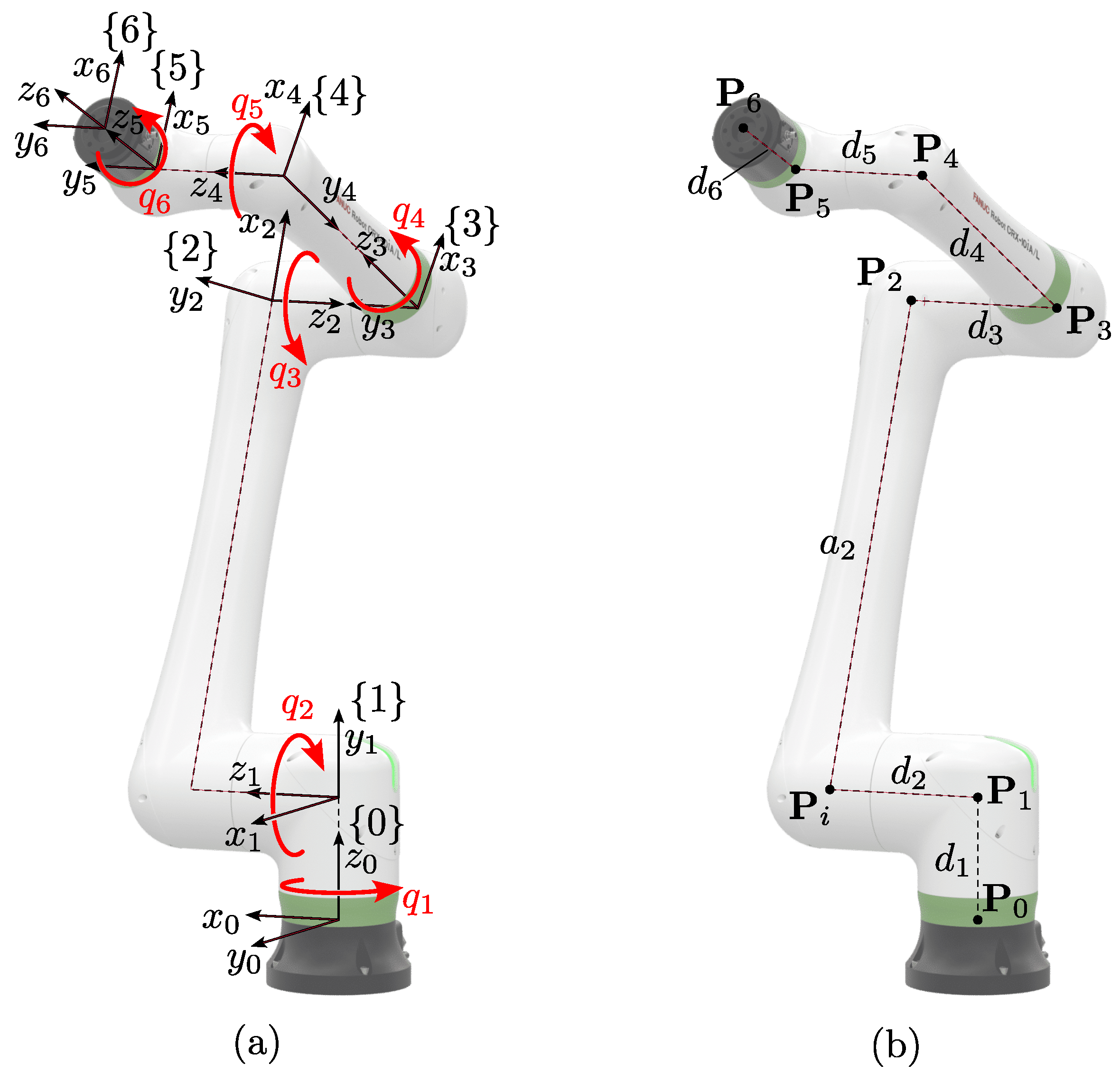
2. Robot Description

A robot of great interest in the collaborative robotics scene is the FANUC CRX-10iA/L (see Figure 1a), which meets industrial reliability requirements and provides all the necessary functionality for human–robot collaboration. In this paper, it is taken as a reference from the family of serial robots with non-spherical wrists, without loss of generality. The kinematic chain of the FANUC CRX-10iA/L is made of six revolute joints (6R) arranged in serial configuration. The first three joints ( J 1 , J 2 and J 3 in Figure 1b) are arranged in a classic kinematic sequence typical of robotic arms while the roll–pitch–roll wrist has a non-spherical configuration. The last three joints ( J 4 , J 5 and J 6 ), in fact, have axes that are two-by-two perpendicular and incident. Moreover, the lack of a common intersection point obviously makes the wrist non-spherical, making it impossible to approach the inverse kinematic problem with the usual methods for serial anthropomorphic manipulators, such as the solution proposed by Pieper [24].
The position and orientation of robot bodies in space are described here with the usual Denavit–Hartenberg notation. It is worth remembering that the mutual position between two frames can be represented by a homogeneous transformation, whose expression is given by:
i T j = cos θ i sin θ i 0 0 sin θ i cos θ i 0 0 0 0 1 d i 0 0 0 1 1 0 0 a i 0 cos α i sin α i 0 0 sin α i cos α i 0 0 0 0 1
where θ i , d i , α i , a i are the well-known Denavit–Hartenberg parameters. In the present case, the actuated joint variables q i are the rotations θ i around the local z-axes.
The FANUC CRX-10iA/L frames are arranged as shown in Figure 2a, while the parameters collected in Table 1 complete their description. The configuration in space of the tool frame { 6 } with respect to the global reference frame { 0 } is obtained by composing the local transformations i T j according to the convention of successive transformation on mobile axes:
0 T 6 = i = 1 6 i 1 T i = 0 T 1 1 T 2 2 T 3 3 T 4 4 T 5 5 T 6

3. Inverse Kinematics Problem

As is well known, the inverse kinematics mapping of a serial chain consists of determining the joint parameters ( q i in the previous notation) able to provide a given pose for the terminal body of the chain (i.e., body 6 in this manuscript, described by frame { 6 } ). It is also well known that such a problem has many real solutions corresponding to the many postures that the robot can exhibit while reaching a given position and orientation of the terminal body.
A usual approach to this problem consists of simply comparing the elements of the final transformation 0 T 6 with a symbolic expression of the same matrix obtained considering unknown the six joint parameters q i :
0 T 6 k i n e m a t i c s i n v e r s e q = q 1 q 2 q 3 q 4 q 5 q 6
This allows the obtaining of a set of 12 equations that can be reduced to six considering that only three elements of the rotational part of the homogeneous transformation matrix are actually independent. Additionally, a common issue in approaching this kind of equation is given by the presence of sines and cosines, which add complexity to the problem. The usual solution is to apply the Weierstrass substitution to have a common parameterization without trigonometric functions, or to treat them (in this case, 12 expressions of cos q i and sin q i for i = 1 , , 6 ) as distinct unknowns related by six further homogeneous equations ( cos 2 q i + sin 2 q i 1 = 0 ). Both strategies lead to a set of polynomial equations of degree 2, whose solution yields to a univariate polynomial: nonetheless, the reduction of such a system is often computationally burdening and the possibility of obtaining a final degree higher than the number of expected results is also significant.
The approach proposed in this manuscript takes into account a different set of unknown variables, hereby collected in a vector called p , which locates the reference frame of one of the robot bodies (frame { 4 } in particular) and, as a result, allows the computation of the coordinates in space of the robot nodal points P i (shown in Figure 2). From such points, then, the computation of the joint variables becomes a trivial issue.
In more detail, the parameterization chosen to express the rotation matrix 0 R 4 between frame { 4 } and the fixed frame { 0 } avoiding trigonometric functions is the Cayley transform, which maps the skew–symmetric matrix C given by:
C = 0 c 3 c 2 c 3 0 c 1 c 2 c 1 0
into a rotation matrix:
0 R 4 = I + C I C 1
Therefore, the shape assumed by the resulting rotation matrix 0 R 4 in terms of the three parameters c i (with i = 1 , 2 , 3 ) is:
0 R 4 = 1 c 1 2 + c 2 2 + c 3 2 + 1 c 1 2 c 2 2 c 3 2 + 1 2 c 1 c 2 2 c 3 2 c 2 + 2 c 1 c 3 2 c 3 + 2 c 1 c 2 c 1 2 + c 2 2 c 3 2 + 1 2 c 2 c 3 2 c 1 2 c 1 c 3 2 c 2 2 c 1 + 2 c 2 c 3 c 1 2 c 2 2 + c 3 2 + 1
Based on such a choice, the Inverse Kinematics Problem actually consists of finding the parameters that allow the determination of the pose of { 4 } (expressed by means of c 1 , c 2 , c 3 and coordinates of P 4 ) starting from { 6 } , and it can be stated as:
0 T 6 k i n e m a t i c s i n v e r s e p = c 1 c 2 c 3 P 4 , x P 4 , y P 4 , z
where the variables c i can be used to describe the orientation of frame { 4 } , as mentioned above, and P 4 , x , P 4 , y , P 4 , z are the coordinates of its origin, gathered in the column vector P 4 . The 6 parameters are then used to build up the needed transformation matrix:
0 T 4 = 0 R 4 P 4 0 1 × 3 1
with obvious meaning of the terms involved. In the following, the system of equations used to work out the solution of the kinematic problem is shown in detail together with its solution path.

3.1. System of Equations

To find the configuration of frame { 4 } once given a value for 0 R 6 , a set of six equations must be provided. To achieve such an aim, it is possible to exploit both the loop-closure of the kinematic chain and the mobility provided by the joint topology. The former can be obtained by considering as known the position in space of points P 5 and P 6 , while the latter is achieved through the mobility of the non-spherical wrist and the anthropomorphic arm.
Starting from the kinematic closure, the coordinates of P 5 are easily obtained via:
P 5 1 = 0 T 6 0 0 d 6 1 = P 5 , x P 5 , y P 5 , z 1
The same point can be written starting from { 4 } in terms of the problem unknowns, namely:
P 5 1 = 0 T 4 0 0 d 5 1
By comparing (9) and (10), the first three equations are obtained. After simplification and elimination of the non-vanishing terms, the three equations obtained are three polynomials in terms of the six unknowns collected in p :
Φ 1 : ( P 4 , x P 5 , x ) ( c 1 2 + c 2 2 + c 3 2 + 1 ) + 2 d 5 ( c 1 c 3 + c 2 ) = 0 Φ 2 : ( P 4 , y P 5 , y ) ( c 1 2 + c 2 2 + c 3 2 + 1 ) + 2 d 5 ( c 2 c 3 c 1 ) = 0 Φ 3 : ( P 4 , z P 5 , z ) ( c 1 2 + c 2 2 + c 3 2 + 1 ) d 5 ( c 1 2 + c 2 2 c 3 2 1 ) = 0
Three additional equations can be worked out from the mobility of frame { 4 } . First, it can be noticed that the y 4 -axis of the frame is constrained to intersect the z 0 -axis of the global coordinate system (since d 2 = d 3 ), except for the case where the two axes are parallel and not coincident, i.e., when the y 4 -axis is directed along vertical and does not pass through the origin of the fixed frame. The latter condition, by the way, is far from the operating conditions of the robot. A more general condition can be stated as the coplanarity of the four points P 0 , P 1 , P 3 and P 4 or better as the linear dependency among the three vectors z 0 , y 4 and ( P 4 P 0 ) . Such a condition is fulfilled when:
det z 0 y 4 ( P 4 P 0 ) = 0
where z 0 = 0 0 1 T , y 4 = 0 R 4 0 1 0 T and ( P 4 P 0 ) = P 4 , x P 4 , y P 4 , z T . After some manipulation and elimination of non-vanishing components, the determinant in (12) can be expanded to obtain the fourth equation of the system:
Φ 4 : ( c 1 2 c 2 2 + c 3 2 1 ) P 4 , x + ( 2 c 1 c 2 2 c 3 ) P 4 , y = 0
The mobility of the kinematic chain, of the wrist in particular, also constrains frame { 4 } to maintain an axis perpendicular to the assigned coordinate system { 6 } , i.e., the axes identified by vectors z 4 and z 6 . The perpendicularity is fulfilled when:
z 4 T z 6 = 0
where z 4 = 0 R 4 0 0 1 T and z 6 is the unit vector of ( P 5 P 6 ) (for the constraint purpose, they can be used interchangeably). After substitution and simplification, the following polynomial is obtained:
Φ 5 : 2 ( c 1 c 3 + c 2 ) ( P 5 , x P 6 , x ) + 2 ( c 2 c 3 c 1 ) ( P 5 , y P 6 , y ) + ( c 1 2 + c 2 2 c 3 2 1 ) ( P 5 , z P 6 , z ) = 0
Finally, it must be noted that point P 3 maintains a constant distance with respect to the center of the robot shoulder, i.e., to the point P 1 . Thus, it is:
( P 3 P 1 ) T ( P 3 P 1 ) a 2 2 = 0
where P 3 = P 4 + 0 R 4 0 d 4 0 T and P 1 = 0 0 d 1 T , yielding the simplified form:
Φ 6 : P 4 , x c 1 2 + c 2 2 + c 3 2 + 1 + 2 d 4 c 1 c 2 c 3 2 + + P 4 , y c 1 2 + c 2 2 + c 3 2 + 1 + d 4 c 1 2 c 2 2 + c 3 2 1 2 + + P 4 , z d 1 c 1 2 + c 2 2 + c 3 2 + 1 + 2 d 4 c 2 c 3 + c 1 2 a 2 2 = 0
The six polynomial equations Φ i must now be solved in the unknown variables of p to obtain a single polynomial in terms of c 1 only. The solution path is detailed in the following section.

3.2. System Solution

At first, it is possible to remove the three Cartesian variables P 4 , x , P 4 , y and P 4 , z exploiting the three equations Φ 1 , Φ 2 and Φ 3 in which they only appear in linear form. Thus, the following expressions can be found in terms of c 1 , c 2 and c 3 :
P 4 , x ( c 1 , c 2 , c 3 ) = P 5 , x d 5 2 ( c 1 c 3 + c 2 ) c 1 2 + c 2 2 + c 3 2 + 1 P 4 , y ( c 1 , c 2 , c 3 ) = P 5 , y d 5 2 ( c 2 c 3 c 1 ) c 1 2 + c 2 2 + c 3 2 + 1 P 4 , z ( c 1 , c 2 , c 3 ) = P 5 , z + d 5 c 1 2 + c 2 2 c 3 2 1 c 1 2 + c 2 2 + c 3 2 + 1
Substitution of (18) into Φ 4 , Φ 5 and Φ 6 yields to a formulation of the robot kinematics in terms of only c 1 , c 2 and c 3 . The resulting polynomials own a maximum degree of 2 and can be expressed as:
Φ h : i , j , k = 0 i + j + k 2 φ h , i j k c 1 i c 2 j c 3 k = 0
where the coefficients φ h , i j k are function of the robot geometric parameters and h = 4 , 5 , 6 . Appendix A shows in detail the value of such coefficients.
To reduce the system of equations and obtain a polynomial in terms of just one of the three unknowns (namely c 1 ), the Equation (19) can be rewritten consequently. To remove c 3 at first, the following shape can be worked out:
X h : k = 0 2 χ h , k c 3 k = 0
where the coefficients χ h , k (detailed in Appendix B) are functions of c 1 and c 2 . It is worth remarking that the formulations (19) and (20) coincide, thus Φ h = X h . However, polynomials (20) can be used to remove c 3 by means of two Sylvester matrices, whose determinants provide two further reduced equations:
Ψ 1 : det χ 4 , 2 χ 4 , 1 χ 4 , 0 0 0 χ 4 , 2 χ 4 , 1 χ 4 , 0 χ 6 , 2 χ 6 , 1 χ 6 , 0 0 0 χ 6 , 2 χ 6 , 1 χ 6 , 0 = 0 Ψ 2 : det χ 5 , 2 χ 5 , 1 χ 5 , 0 0 0 χ 5 , 2 χ 5 , 1 χ 5 , 0 χ 6 , 2 χ 6 , 1 χ 6 , 0 0 0 χ 6 , 2 χ 6 , 1 χ 6 , 0 = 0
The vanishing set of the determinants Ψ 1 and Ψ 2 (which are polynomials of c 1 and c 2 ) represent the solution to the inverse kinematics problem. The maximum degree of the polynomials is 4 and in compact form they can be formulated as:
Ψ h : i , j = 0 i + j 4 ψ h , i j c 1 i c 2 j = 0
The elimination via Sylvester matrix can be adopted also to remove the unknown c 2 by rewriting (22) as:
Ω h : j = 0 4 ω h , j c 2 j = 0
Again, it is remarked that (23) is a different formulation of (22), nevertheless Ψ h = Ω h . A complete formulation of coefficients ω h , j is provided in Appendix C, where they are presented already as polynomials of the only unknown c 1 .
The last step of the solution is made using again the Sylvester method for reduction of variable c 2 by means of (23). A further matrix is built, whose determinant is a polynomial of degree 16 in terms of the only unknown c 1 :
Λ : det ω 1 , 4 ω 1 , 3 ω 1 , 2 ω 1 , 1 ω 1 , 0 0 0 0 0 ω 1 , 4 ω 1 , 3 ω 1 , 2 ω 1 , 1 ω 1 , 0 0 0 0 0 ω 1 , 4 ω 1 , 3 ω 1 , 2 ω 1 , 1 ω 1 , 0 0 0 0 0 ω 1 , 4 ω 1 , 3 ω 1 , 2 ω 1 , 1 ω 1 , 0 ω 2 , 4 ω 2 , 3 ω 2 , 2 ω 2 , 1 ω 2 , 0 0 0 0 0 ω 2 , 4 ω 2 , 3 ω 2 , 2 ω 2 , 1 ω 2 , 0 0 0 0 0 ω 2 , 4 ω 2 , 3 ω 2 , 2 ω 2 , 1 ω 2 , 0 0 0 0 0 ω 2 , 4 ω 2 , 3 ω 2 , 2 ω 2 , 1 ω 2 , 0 = 0
In more compact form, the solving equation Λ is:
Λ : i = 0 16 λ i c 1 i = 0
where the coefficients λ i for i = 1 , , 16 are finally functions of only geometric parameters. Unfortunately, explicit expressions for the coefficients are too large to be shown in this document. Nonetheless, Appendix D shows (25) in terms of the polynomials ω h , i appearing in matrix (24). The polynomial provides up to 16 real solutions to the problem, corresponding to its roots. The number of solutions does not change depending on proximity to singular poses or joint limits. However, it obviously becomes equal to 0 for singular configurations (such as any point out of the robot workspace) for which only complex roots can be found (25). In the remainder of the manuscript, details are provided about the back-substitution of such values and the numeric implementation for the computation of the other variables of the problem.

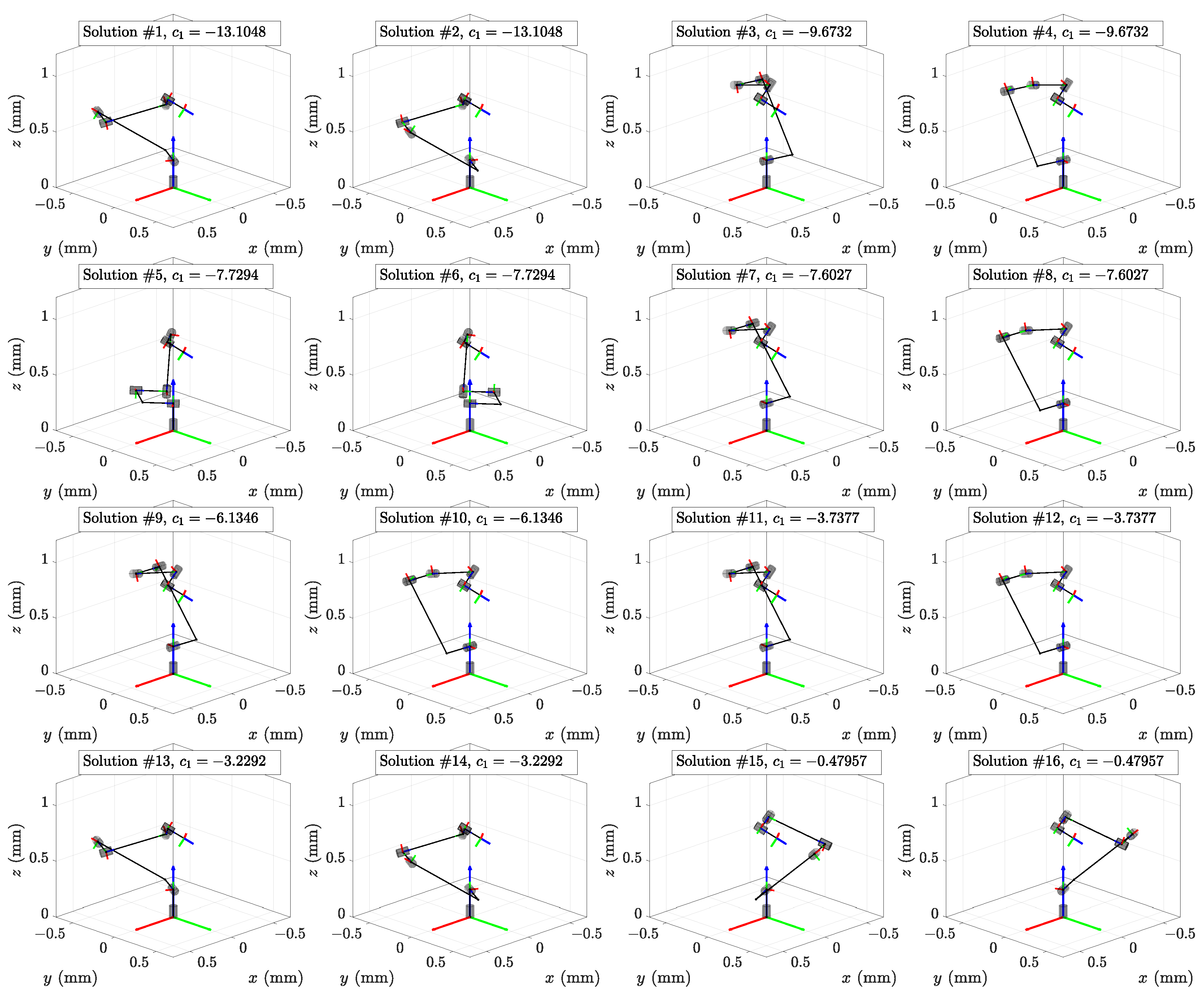
4. Implementation and Verification

As aforementioned, the vanishing set of the polynomial (25) allows the discovery of up to 16 real solutions for the inverse kinematics problem, corresponding to the roots of Λ . The expanded equations shown in the appendices provide an impression of the coefficient dimensions that cannot be further reduced. For this reason, the products of polynomials ω h , i have not been made explicit during the implementation of the inverse kinematics algorithm. On the contrary, the coefficients of Λ have been obtained as a sum of the coefficients of each addendum appearing in Appendix D, and each of them was worked out via the convolution of the corresponding discrete sequence of coefficients.
As is known, in fact, given two polynomials f ( x ) and g ( x ) of degree m and n, respectively:
f ( x ) = i = 0 m f i x i g ( x ) = i = 0 n g i x i
the product f ( x ) g ( x ) is a m + n degree polynomial given by:
h ( x ) = f ( x ) g ( x ) = i = 0 m + n h i x i with h i = k = 0 i f k g i k
The definition of h i can be easily extended to a , + sum, and then to a definition of the convolution of a discrete series. Therefore, the coefficients h i of polynomial h ( x ) = f ( x ) g ( x ) are computable as the convolution f i g i . Let us take, for example, the multiplication ω 1 , 3 ω 2 , 2 . The coefficients of the resulting polynomial will be provided by the convolution of the coefficients of the factors, thus:
ω 1 , 3 ω 2 , 2 = B 1 , C 1 c 1 1 D 2 , E 2 , F 2 c 1 2 c 1 1 = B 1 , C 1 D 2 , E 2 , F 2 c 1 3 c 1 2 c 1 1
where expressions in terms of the robot geometric parameters are provided in the appendices for A i , B i , C i , etc.
Using convolution rather than multiplication allows computation with relative ease of the coefficients of Λ and therefore its 16 roots. Then, the remaining unknowns can be computed following the solution path backwards and substituting the values obtained time by time. Starting from (24), a linear system of equation can be built as:
ω 1 , 4 ω 1 , 3 ω 1 , 2 ω 1 , 1 ω 1 , 0 0 0 ω 1 , 4 ω 1 , 3 ω 1 , 2 ω 1 , 1 ω 1 , 0 0 0 ω 1 , 4 ω 1 , 3 ω 1 , 2 ω 1 , 1 ω 2 , 4 ω 2 , 3 ω 2 , 2 ω 2 , 1 ω 2 , 0 0 0 ω 2 , 4 ω 2 , 3 ω 2 , 2 ω 2 , 1 ω 2 , 0 0 0 ω 2 , 4 ω 2 , 3 ω 2 , 2 ω 2 , 1 c 2 6 c 2 5 c 2 4 c 2 3 c 2 2 c 2 = 0 0 ω 1 , 0 0 0 ω 2 , 0
Substituting one at a time the 16 values of c 1 (corresponding to the roots of Λ ) to evaluate the polynomials ω h , i , the respective values of c 2 can be found from a solution of (29). As c 1 and c 2 are now known, the coefficients χ h , k of (20) can be computed and used to obtain c 3 picking two equations from the three X h . For example, it is possible to formulate the linear system:
χ 4 , 2 χ 4 , 1 χ 5 , 2 χ 5 , 1 c 3 2 c 3 = χ 4 , 0 χ 5 , 0
Lastly, the three orientation parameters c 1 , c 2 and c 3 can be substituted into (18) to obtain the coordinates P 4 , x , P 4 , y , P 4 , z of the origin of the reference frame { 4 } . This passage almost closes the inverse kinematics problem, although the last few steps of joint variables computation are still at stake. To provide a complete mapping 0 T 6 q , the coordinates of the points P 4 and P 3 = P 4 + 0 R 4 0 d 4 0 T can be exploited. The passages to obtain the values of the joint variables, which are quite trivial, are not shown here for the sake of conciseness, although their full formulation is shown in Appendix E. However, it is worth remarking that their values are calculated in cascade, following the order q 2 , q 1 , q 3 , q 4 , q 5 , q 6 .
It is also worth noting that the very first computation, i.e., q 2 = arcsin ( P 3 , x P 1 , x ) / a 2 , doubles the number of available solutions (being acceptable both q 2 and π q 2 ). Actually, the solutions obtained considering the full domain of the function arcsin are already present within the set of points coordinates previously found. In practice, applying in sequence the mapping 0 T 6 p and p q duplicated solutions are added to the available ones (that can be easily eliminated).

Numerical Example

Finally, to verify the effectiveness of the proposed solution, a numerical example is shown. A random set of joint angles is picked to compute the robot forward kinematics by (2). In particular, in degrees:
q = 78 131 24 42 60 10 T
which provide the transformation matrix:
0 T 6 = 0.3363 0.8387 0.4283 0.0571 0.6182 0.1464 0.7722 0.1786 0.7104 0.5245 0.4693 0.7677 0 0 0 1
The resulting known points useful for inverse kinematics computations and for results check are (in mm):
P 0 = 0.0 0.0 0.0 P 1 = 0.0 0.0 250.3 P 3 = 125.7 55.0 842.7 P 4 = 0.0 0.0 250.3 P 5 = 125.7 55.0 842.7 P 6 = 57.1 178.6 767.7
Such coordinates, together with the geometrical parameters already introduced in Table 1, can be substituted into the explicit expressions of the coefficients of polynomials ω h , i . Such polynomials allow computing, via convolution, the coefficients of Λ , whose roots represent the values of c 1 which are the solution of the inverse kinematics problem. Substituting in cascade into (29), (30) and (18), it is possible to obtain the values of the remaining unknowns, which are shown in Table 2. As is shown, the polynomial Λ provides in this case only eight real solutions, for which it is possible to evaluate eight poses for the reference frame { 4 } .
The results offered by the algorithm in terms of pose of { 4 } can be then mapped into sets of joint variables by means of the equations presented in Appendix D. As aforementioned, the eight real solutions of c 1 are doubled by the angle computations (see Table 3), although four of the resulting configurations (shown in Figure 3) are repeated.

5. Conclusions

This manuscript proposes a closed-form solution for the inverse kinematics mapping of a class of 6R robotic manipulators, characterized by a non-spherical wrist. On the one hand, such a feature improves the robot mechanical simplicity and provides some advantage in terms of dexterity; on the other, it prevents the use of common methods developed for anthropomorphic arms. For this reason, a specific approach has been worked out based on the constraint equations that characterize the mobility of an inner body of the kinematic chain (i.e., the first body of the non-spherical wrist). The solution path eliminates one at a time five out of the six unknowns of the problem and provides a univariate polynomial of degree 16, whose roots represent the problem solution. Backward substitution and computation of the actuated joint angles are shown to close the solution path and provide a full map of the end-effector configurations space and the motors space. In conclusion, the manuscript provides a complete walk-through to compute all the possible postures that the FANUC CRX family of cobots can exhibit to reach a given pose. Obviously, the proposed method is effective also for all the manipulators sharing their joint topology with the FANUC CRX family, i.e., for those manipulators for which the written equations are valid. Future developments will involve the analysis of the robot workspace to also provide a complete map of robot workspace boundaries and inner singularities, the analysis of representation singularities, and the impact of the problem of numerical conditioning on the accuracy of the kinematics solution.

Author Contributions

Conceptualization, L.C. and M.-C.P.; methodology, L.C.; software, L.C.; validation, L.C.; formal analysis, L.C., M.-C.P. and M.C.; investigation, L.C.; resources, M.C.; data curation, L.C.; writing—original draft preparation, L.C.; writing—review and editing, M.-C.P. and M.C.; visualization, M.-C.P.; supervision, M.C.; project administration, L.C.; funding acquisition, M.-C.P. and M.C. All authors have read and agreed to the published version of the manuscript.

Funding

This research received no external funding.

Institutional Review Board Statement

Not applicable.

Informed Consent Statement

Not applicable.

Data Availability Statement

Not applicable.

Conflicts of Interest

The authors declare no conflict of interest.

Appendix A. Coefficients of Polynomials Φh

φ 4 , 002 = P 5 , x φ 4 , 011 = 0 φ 4 , 101 = 2 d 5 φ 4 , 001 = 2 P 5 , y φ 4 , 020 = P 5 , x φ 4 , 110 = 2 P 5 , y φ 4 , 010 = 2 d 5 φ 4 , 200 = P 5 , x φ 4 , 100 = 0 φ 4 , 000 = P 5 , x φ 5 , 002 = P 5 , z P 6 , z φ 5 , 011 = 2 P 5 , y 2 P 6 , y φ 5 , 101 = 2 P 5 , x 2 P 6 , x φ 5 , 001 = 0 φ 5 , 020 = P 6 , z P 5 , z φ 5 , 110 = 0 φ 5 , 010 = 2 P 5 , x 2 P 6 , x φ 5 , 200 = P 6 , z P 5 , z φ 5 , 100 = 2 P 6 , y 2 P 5 , y φ 5 , 000 = P 5 , z P 6 , z φ 6 , 002 = P 5 , x 2 + P 5 , y 2 + P 5 , z 2 2 P 5 , y d 4 2 P 5 , z ( d 1 + d 5 ) d 2 2 + d 1 2 + 2 d 1 d 5 + d 4 2 + d 5 2 φ 6 , 011 = 4 P 5 , z d 4 4 P 5 , y d 5 4 d 1 d 4 φ 6 , 101 = 4 P 5 , x d 5 φ 6 , 001 = 4 P 5 , x d 4 φ 6 , 020 = P 5 , x 2 + P 5 , y 2 + P 5 , z 2 + 2 P 5 , y d 4 2 P 5 , z ( d 1 d 5 ) d 2 2 + d 1 2 2 d 1 d 5 + d 4 2 + d 5 2 φ 6 , 110 = 4 P 5 , x d 4 φ 6 , 010 = 4 P 5 , x d 5 φ 6 , 200 = P 5 , x 2 + P 5 , y 2 + P 5 , z 2 2 P 5 , y d 4 2 P 5 , z ( d 1 + d 5 ) d 2 2 + d 1 2 2 d 1 d 5 + d 4 2 + d 5 2 φ 6 , 100 = 4 P 5 , y d 5 + 4 P 5 , z d 4 4 d 1 d 4 φ 6 , 000 = P 5 , x 2 + P 5 , y 2 + P 5 , z 2 + 2 P 5 , y d 4 2 P 5 , z ( d 1 + d 5 ) d 2 2 + d 1 2 + 2 d 1 d 5 + d 4 2 + d 5 2

Appendix B. Coefficients of Polynomials Xh

χ h , 2 = φ h , 002 χ h , 1 = φ h , 001 + φ h , 101 c 1 + φ h , 011 c 2 χ h , 0 = φ h , 200 c 1 2 + φ h , 110 c 1 c 2 + φ h , 100 c 1 + φ h , 020 c 2 2 + φ h , 010 c 2 + φ h , 000

Appendix C. Coefficients of Polynomials Ωh

ω h , 4 = A h ω h , 3 = B h c 1 + C h ω h , 2 = D h c 1 2 + E h c 1 + F h ω h , 1 = G h c 1 3 + H h c 1 2 + I h c 1 + J h ω h , 0 = K h c 1 4 + L h c 1 3 + M h c 1 2 + N h c 1 + O h
In the following, h * = 4 for h = 1 and h * = 5 for h = 2 .
A h = φ h * , 002 2 φ 6 , 020 2 φ h * , 002 φ h * , 011 φ 6 , 011 φ 6 , 020 2 φ h * , 002 φ h * , 020 φ 6 , 002 φ 6 , 020 + φ h * , 002 φ h * , 020 φ 6 , 011 2 + φ h * , 011 2 φ 6 , 002 φ 6 , 020 φ h * , 011 φ h * , 020 φ 6 , 002 φ 6 , 011 + φ h * , 020 2 φ 6 , 002 2 B h = φ h * , 002 φ h * , 110 φ 6 , 011 2 + 2 φ h * , 020 φ h * , 110 φ 6 , 002 2 + φ h * , 011 2 φ 6 , 002 φ 6 , 110 + 2 φ h * , 002 2 φ 6 , 020 φ 6 , 110 φ h * , 002 φ h * , 011 φ 6 , 011 φ 6 , 110 φ h * , 002 φ h * , 011 φ 6 , 020 φ 6 , 101 2 φ h * , 002 φ h * , 020 φ 6 , 002 φ 6 , 110 + 2 φ h * , 002 φ h * , 020 φ 6 , 011 φ 6 , 101 φ h * , 002 φ h * , 101 φ 6 , 011 φ 6 , 020 2 φ h * , 002 φ h * , 110 φ 6 , 002 φ 6 , 020 φ h * , 011 φ h * , 020 φ 6 , 002 φ 6 , 101 + 2 φ h * , 011 φ h * , 101 φ 6 , 002 φ 6 , 020 φ h * , 011 φ h * , 110 φ 6 , 002 φ 6 , 011 φ h * , 020 φ h * , 101 φ 6 , 002 φ 6 , 011 C h = φ h * , 002 φ h * , 010 φ 6 , 011 2 + 2 φ h * , 010 φ h * , 020 φ 6 , 002 2 + φ h * , 011 2 φ 6 , 002 φ 6 , 010 + 2 φ h * , 002 2 φ 6 , 010 φ 6 , 020 φ h * , 001 φ h * , 002 φ 6 , 011 φ 6 , 020 + 2 φ h * , 001 φ h * , 011 φ 6 , 002 φ 6 , 020 φ h * , 001 φ h * , 020 φ 6 , 002 φ 6 , 011 2 φ h * , 002 φ h * , 010 φ 6 , 002 φ 6 , 020 φ h * , 002 φ h * , 011 φ 6 , 001 φ 6 , 020 φ h * , 002 φ h * , 011 φ 6 , 010 φ 6 , 011 + 2 φ h * , 002 φ h * , 020 φ 6 , 001 φ 6 , 011 2 φ h * , 002 φ h * , 020 φ 6 , 002 φ 6 , 010 φ h * , 010 φ h * , 011 φ 6 , 002 φ 6 , 011 φ h * , 011 φ h * , 020 φ 6 , 001 φ 6 , 002 D h = φ h * , 002 2 φ 6 , 110 2 + φ h * , 110 2 φ 6 , 002 2 + φ h * , 002 φ h * , 020 φ 6 , 101 2 + φ h * , 002 φ h * , 200 φ 6 , 011 2 + 2 φ h * , 020 φ h * , 200 φ 6 , 002 2 + φ h * , 101 2 φ 6 , 002 φ 6 , 020 + φ h * , 011 2 φ 6 , 002 φ 6 , 200 + 2 φ h * , 002 2 φ 6 , 020 φ 6 , 200 φ h * , 002 φ h * , 011 φ 6 , 011 φ 6 , 200 φ h * , 002 φ h * , 011 φ 6 , 101 φ 6 , 110 2 φ h * , 002 φ h * , 020 φ 6 , 002 φ 6 , 200 φ h * , 002 φ h * , 101 φ 6 , 011 φ 6 , 110 φ h * , 002 φ h * , 101 φ 6 , 020 φ 6 , 101 2 φ h * , 002 φ h * , 110 φ 6 , 002 φ 6 , 110 + 2 φ h * , 002 φ h * , 110 φ 6 , 011 φ 6 , 101 2 φ h * , 002 φ h * , 200 φ 6 , 002 φ 6 , 020 + 2 φ h * , 011 φ h * , 101 φ 6 , 002 φ 6 , 110 φ h * , 011 φ h * , 110 φ 6 , 002 φ 6 , 101 φ h * , 011 φ h * , 200 φ 6 , 002 φ 6 , 011 φ h * , 020 φ h * , 101 φ 6 , 002 φ 6 , 101 φ h * , 101 φ h * , 110 φ 6 , 002 φ 6 , 011 E h = φ h * , 002 φ h * , 100 φ 6 , 011 2 + 2 φ h * , 010 φ h * , 110 φ 6 , 002 2 + 2 φ h * , 020 φ h * , 100 φ 6 , 002 2 + φ h * , 011 2 φ 6 , 002 φ 6 , 100 + 2 φ h * , 002 2 φ 6 , 010 φ 6 , 110 + 2 φ h * , 002 2 φ 6 , 020 φ 6 , 100 φ h * , 001 φ h * , 002 φ 6 , 011 φ 6 , 110 φ h * , 001 φ h * , 002 φ 6 , 020 φ 6 , 101 + 2 φ h * , 001 φ h * , 011 φ 6 , 002 φ 6 , 110 φ h * , 001 φ h * , 020 φ 6 , 002 φ 6 , 101 + 2 φ h * , 001 φ h * , 101 φ 6 , 002 φ 6 , 020 φ h * , 001 φ h * , 110 φ 6 , 002 φ 6 , 011 2 φ h * , 002 φ h * , 010 φ 6 , 002 φ 6 , 110 + 2 φ h * , 002 φ h * , 010 φ 6 , 011 φ 6 , 101 φ h * , 002 φ h * , 011 φ 6 , 001 φ 6 , 110 φ h * , 002 φ h * , 011 φ 6 , 010 φ 6 , 101 φ h * , 002 φ h * , 011 φ 6 , 011 φ 6 , 100 + 2 φ h * , 002 φ h * , 020 φ 6 , 001 φ 6 , 101 2 φ h * , 002 φ h * , 020 φ 6 , 002 φ 6 , 100 2 φ h * , 002 φ h * , 100 φ 6 , 002 φ 6 , 020 φ h * , 002 φ h * , 101 φ 6 , 001 φ 6 , 020 φ h * , 002 φ h * , 101 φ 6 , 010 φ 6 , 011 + 2 φ h * , 002 φ h * , 110 φ 6 , 001 φ 6 , 011 2 φ h * , 002 φ h * , 110 φ 6 , 002 φ 6 , 010 φ h * , 010 φ h * , 011 φ 6 , 002 φ 6 , 101 φ h * , 010 φ h * , 101 φ 6 , 002 φ 6 , 011 φ h * , 011 φ h * , 100 φ 6 , 002 φ 6 , 011 + 2 φ h * , 011 φ h * , 101 φ 6 , 002 φ 6 , 010 φ h * , 011 φ h * , 110 φ 6 , 001 φ 6 , 002 φ h * , 020 φ h * , 101 φ 6 , 001 φ 6 , 002 F h = φ h * , 002 2 φ 6 , 010 2 + φ h * , 010 2 φ 6 , 002 2 + φ h * , 000 φ h * , 002 φ 6 , 011 2 + 2 φ h * , 000 φ h * , 020 φ 6 , 002 2 + φ h * , 002 φ h * , 020 φ 6 , 001 2 + φ h * , 011 2 φ 6 , 000 φ 6 , 002 + 2 φ h * , 002 2 φ 6 , 000 φ 6 , 020 + φ h * , 001 2 φ 6 , 002 φ 6 , 020 2 φ h * , 000 φ h * , 002 φ 6 , 002 φ 6 , 020 φ h * , 000 φ h * , 011 φ 6 , 002 φ 6 , 011 φ h * , 001 φ h * , 002 φ 6 , 001 φ 6 , 020 φ h * , 001 φ h * , 002 φ 6 , 010 φ 6 , 011 φ h * , 001 φ h * , 010 φ 6 , 002 φ 6 , 011 + 2 φ h * , 001 φ h * , 011 φ 6 , 002 φ 6 , 010 φ h * , 001 φ h * , 020 φ 6 , 001 φ 6 , 002 + 2 φ h * , 002 φ h * , 010 φ 6 , 001 φ 6 , 011 2 φ h * , 002 φ h * , 010 φ 6 , 002 φ 6 , 010 φ h * , 002 φ h * , 011 φ 6 , 000 φ 6 , 011 φ h * , 002 φ h * , 011 φ 6 , 001 φ 6 , 010 2 φ h * , 002 φ h * , 020 φ 6 , 000 φ 6 , 002 φ h * , 010 φ h * , 011 φ 6 , 001 φ 6 , 002
G h = φ h * , 002 φ h * , 110 φ 6 , 101 2 + 2 φ h * , 110 φ h * , 200 φ 6 , 002 2 + φ h * , 101 2 φ 6 , 002 φ 6 , 110 + 2 φ h * , 002 2 φ 6 , 110 φ 6 , 200 φ h * , 002 φ h * , 011 φ 6 , 101 φ 6 , 200 φ h * , 002 φ h * , 101 φ 6 , 011 φ 6 , 200 φ h * , 002 φ h * , 101 φ 6 , 101 φ 6 , 110 2 φ h * , 002 φ h * , 110 φ 6 , 002 φ 6 , 200 2 φ h * , 002 φ h * , 200 φ 6 , 002 φ 6 , 110 + 2 φ h * , 002 φ h * , 200 φ 6 , 011 φ 6 , 101 + 2 φ h * , 011 φ h * , 101 φ 6 , 002 φ 6 , 200 φ h * , 011 φ h * , 200 φ 6 , 002 φ 6 , 101 φ h * , 101 φ h * , 110 φ 6 , 002 φ 6 , 101 φ h * , 101 φ h * , 200 φ 6 , 002 φ 6 , 011 H h = φ h * , 002 φ h * , 010 φ 6 , 101 2 + 2 φ h * , 010 φ h * , 200 φ 6 , 002 2 + 2 φ h * , 100 φ h * , 110 φ 6 , 002 2 + φ h * , 101 2 φ 6 , 002 φ 6 , 010 + 2 φ h * , 002 2 φ 6 , 010 φ 6 , 200 + 2 φ h * , 002 2 φ 6 , 100 φ 6 , 110 φ h * , 001 φ h * , 002 φ 6 , 011 φ 6 , 200 φ h * , 001 φ h * , 002 φ 6 , 101 φ 6 , 110 + 2 φ h * , 001 φ h * , 011 φ 6 , 002 φ 6 , 200 + 2 φ h * , 001 φ h * , 101 φ 6 , 002 φ 6 , 110 φ h * , 001 φ h * , 110 φ 6 , 002 φ 6 , 101 φ h * , 001 φ h * , 200 φ 6 , 002 φ 6 , 011 2 φ h * , 002 φ h * , 010 φ 6 , 002 φ 6 , 200 φ h * , 002 φ h * , 011 φ 6 , 001 φ 6 , 200 φ h * , 002 φ h * , 011 φ 6 , 100 φ 6 , 101 2 φ h * , 002 φ h * , 100 φ 6 , 002 φ 6 , 110 + 2 φ h * , 002 φ h * , 100 φ 6 , 011 φ 6 , 101 φ h * , 002 φ h * , 101 φ 6 , 001 φ 6 , 110 φ h * , 002 φ h * , 101 φ 6 , 010 φ 6 , 101 φ h * , 002 φ h * , 101 φ 6 , 011 φ 6 , 100 + 2 φ h * , 002 φ h * , 110 φ 6 , 001 φ 6 , 101 2 φ h * , 002 φ h * , 110 φ 6 , 002 φ 6 , 100 + 2 φ h * , 002 φ h * , 200 φ 6 , 001 φ 6 , 011 2 φ h * , 002 φ h * , 200 φ 6 , 002 φ 6 , 010 φ h * , 010 φ h * , 101 φ 6 , 002 φ 6 , 101 φ h * , 011 φ h * , 100 φ 6 , 002 φ 6 , 101 + 2 φ h * , 011 φ h * , 101 φ 6 , 002 φ 6 , 100 φ h * , 011 φ h * , 200 φ 6 , 001 φ 6 , 002 φ h * , 100 φ h * , 101 φ 6 , 002 φ 6 , 011 φ h * , 101 φ h * , 110 φ 6 , 001 φ 6 , 002 I h = 2 φ h * , 000 φ h * , 110 φ 6 , 002 2 + 2 φ h * , 010 φ h * , 100 φ 6 , 002 2 + φ h * , 002 φ h * , 110 φ 6 , 001 2 + 2 φ h * , 002 2 φ 6 , 000 φ 6 , 110 + 2 φ h * , 002 2 φ 6 , 010 φ 6 , 100 + φ h * , 001 2 φ 6 , 002 φ 6 , 110 2 φ h * , 000 φ h * , 002 φ 6 , 002 φ 6 , 110 + 2 φ h * , 000 φ h * , 002 φ 6 , 011 φ 6 , 101 φ h * , 000 φ h * , 011 φ 6 , 002 φ 6 , 101 φ h * , 000 φ h * , 101 φ 6 , 002 φ 6 , 011 φ h * , 001 φ h * , 002 φ 6 , 001 φ 6 , 110 φ h * , 001 φ h * , 002 φ 6 , 010 φ 6 , 101 φ h * , 001 φ h * , 002 φ 6 , 011 φ 6 , 100 φ h * , 001 φ h * , 010 φ 6 , 002 φ 6 , 101 + 2 φ h * , 001 φ h * , 011 φ 6 , 002 φ 6 , 100 φ h * , 001 φ h * , 100 φ 6 , 002 φ 6 , 011 + 2 φ h * , 001 φ h * , 101 φ 6 , 002 φ 6 , 010 φ h * , 001 φ h * , 110 φ 6 , 001 φ 6 , 002 + 2 φ h * , 002 φ h * , 010 φ 6 , 001 φ 6 , 101 2 φ h * , 002 φ h * , 010 φ 6 , 002 φ 6 , 100 φ h * , 002 φ h * , 011 φ 6 , 000 φ 6 , 101 φ h * , 002 φ h * , 011 φ 6 , 001 φ 6 , 100 + 2 φ h * , 002 φ h * , 100 φ 6 , 001 φ 6 , 011 2 φ h * , 002 φ h * , 100 φ 6 , 002 φ 6 , 010 φ h * , 002 φ h * , 101 φ 6 , 000 φ 6 , 011 φ h * , 002 φ h * , 101 φ 6 , 001 φ 6 , 010 2 φ h * , 002 φ h * , 110 φ 6 , 000 φ 6 , 002 φ h * , 010 φ h * , 101 φ 6 , 001 φ 6 , 002 φ h * , 011 φ h * , 100 φ 6 , 001 φ 6 , 002 + 2 φ h * , 011 φ h * , 101 φ 6 , 000 φ 6 , 002 J h = 2 φ h * , 000 φ h * , 010 φ 6 , 002 2 + φ h * , 002 φ h * , 010 φ 6 , 001 2 + 2 φ h * , 002 2 φ 6 , 000 φ 6 , 010 + φ h * , 001 2 φ 6 , 002 φ 6 , 010 φ h * , 000 φ h * , 001 φ 6 , 002 φ 6 , 011 + 2 φ h * , 000 φ h * , 002 φ 6 , 001 φ 6 , 011 2 φ h * , 000 φ h * , 002 φ 6 , 002 φ 6 , 010 φ h * , 000 φ h * , 011 φ 6 , 001 φ 6 , 002 φ h * , 001 φ h * , 002 φ 6 , 000 φ 6 , 011 φ h * , 001 φ h * , 002 φ 6 , 001 φ 6 , 010 φ h * , 001 φ h * , 010 φ 6 , 001 φ 6 , 002 + 2 φ h * , 001 φ h * , 011 φ 6 , 000 φ 6 , 002 2 φ h * , 002 φ h * , 010 φ 6 , 000 φ 6 , 002 φ h * , 002 φ h * , 011 φ 6 , 000 φ 6 , 001 K h = φ h * , 002 2 φ 6 , 200 2 φ h * , 002 φ h * , 101 φ 6 , 101 φ 6 , 200 2 φ h * , 002 φ h * , 200 φ 6 , 002 φ 6 , 200 + φ h * , 002 φ h * , 200 φ 6 , 101 2 + φ h * , 101 2 φ 6 , 002 φ 6 , 200 φ h * , 101 φ h * , 200 φ 6 , 002 φ 6 , 101 + φ h * , 200 2 φ 6 , 002 2 L h = φ h * , 002 φ h * , 100 φ 6 , 101 2 + 2 φ h * , 100 φ h * , 200 φ 6 , 002 2 + φ h * , 101 2 φ 6 , 002 φ 6 , 100 + 2 φ h * , 002 2 φ 6 , 100 φ 6 , 200 φ h * , 001 φ h * , 002 φ 6 , 101 φ 6 , 200 + 2 φ h * , 001 φ h * , 101 φ 6 , 002 φ 6 , 200 φ h * , 001 φ h * , 200 φ 6 , 002 φ 6 , 101 2 φ h * , 002 φ h * , 100 φ 6 , 002 φ 6 , 200 φ h * , 002 φ h * , 101 φ 6 , 001 φ 6 , 200 φ h * , 002 φ h * , 101 φ 6 , 100 φ 6 , 101 + 2 φ h * , 002 φ h * , 200 φ 6 , 001 φ 6 , 101 2 φ h * , 002 φ h * , 200 φ 6 , 002 φ 6 , 100 φ h * , 100 φ h * , 101 φ 6 , 002 φ 6 , 101 φ h * , 101 φ h * , 200 φ 6 , 001 φ 6 , 002 M h = φ h * , 002 2 φ 6 , 100 2 + φ h * , 100 2 φ 6 , 002 2 + φ h * , 000 φ h * , 002 φ 6 , 101 2 + 2 φ h * , 000 φ h * , 200 φ 6 , 002 2 + φ h * , 002 φ h * , 200 φ 6 , 001 2 + φ h * , 101 2 φ 6 , 000 φ 6 , 002 + 2 φ h * , 002 2 φ 6 , 000 φ 6 , 200 + φ h * , 001 2 φ 6 , 002 φ 6 , 200 2 φ h * , 000 φ h * , 002 φ 6 , 002 φ 6 , 200 φ h * , 000 φ h * , 101 φ 6 , 002 φ 6 , 101 φ h * , 001 φ h * , 002 φ 6 , 001 φ 6 , 200 φ h * , 001 φ h * , 002 φ 6 , 100 φ 6 , 101 φ h * , 001 φ h * , 100 φ 6 , 002 φ 6 , 101 + 2 φ h * , 001 φ h * , 101 φ 6 , 002 φ 6 , 100 φ h * , 001 φ h * , 200 φ 6 , 001 φ 6 , 002 + 2 φ h * , 002 φ h * , 100 φ 6 , 001 φ 6 , 101 2 φ h * , 002 φ h * , 100 φ 6 , 002 φ 6 , 100 φ h * , 002 φ h * , 101 φ 6 , 000 φ 6 , 101 φ h * , 002 φ h * , 101 φ 6 , 001 φ 6 , 100 2 φ h * , 002 φ h * , 200 φ 6 , 000 φ 6 , 002 φ h * , 100 φ h * , 101 φ 6 , 001 φ 6 , 002 N h = 2 φ h * , 000 φ h * , 100 φ 6 , 002 2 + φ h * , 002 φ h * , 100 φ 6 , 001 2 + 2 φ h * , 002 2 φ 6 , 000 φ 6 , 100 + φ h * , 001 2 φ 6 , 002 φ 6 , 100 φ h * , 000 φ h * , 001 φ 6 , 002 φ 6 , 101 + 2 φ h * , 000 φ h * , 002 φ 6 , 001 φ 6 , 101 2 φ h * , 000 φ h * , 002 φ 6 , 002 φ 6 , 100 φ h * , 000 φ h * , 101 φ 6 , 001 φ 6 , 002 φ h * , 001 φ h * , 002 φ 6 , 000 φ 6 , 101 φ h * , 001 φ h * , 002 φ 6 , 001 φ 6 , 100 φ h * , 001 φ h * , 100 φ 6 , 001 φ 6 , 002 + 2 φ h * , 001 φ h * , 101 φ 6 , 000 φ 6 , 002 2 φ h * , 002 φ h * , 100 φ 6 , 000 φ 6 , 002 φ h * , 002 φ h * , 101 φ 6 , 000 φ 6 , 001 O h = φ h * , 000 2 φ 6 , 002 2 φ h * , 000 φ h * , 001 φ 6 , 001 φ 6 , 002 2 φ h * , 000 φ h * , 002 φ 6 , 000 φ 6 , 002 + φ h * , 000 φ h * , 002 φ 6 , 001 2 + φ h * , 001 2 φ 6 , 000 φ 6 , 002 φ h * , 001 φ h * , 002 φ 6 , 000 φ 6 , 001 + φ h * , 002 2 φ 6 , 000 2

Appendix D. Univariate Polynomial

Λ : ω 1 , 4 4 ω 2 , 0 4 + ω 1 , 0 4 ω 2 , 4 4 + ω 1 , 4 2 ω 1 , 0 2 ω 2 , 2 4 + ω 1 , 2 4 ω 2 , 4 2 ω 2 , 0 2 + ω 1 , 4 ω 1 , 0 3 ω 2 , 3 4 + ω 1 , 4 3 ω 1 , 0 ω 2 , 1 4 + ω 1 , 3 4 ω 2 , 4 ω 2 , 0 3 + ω 1 , 1 4 ω 2 , 4 3 ω 2 , 0 ω 1 , 4 ω 1 , 3 3 ω 2 , 3 ω 2 , 0 3 ω 1 , 3 ω 1 , 0 3 ω 2 , 4 ω 2 , 3 3 ω 1 , 4 ω 1 , 1 3 ω 2 , 3 3 ω 2 , 0 4 ω 1 , 4 ω 1 , 0 3 ω 2 , 4 3 ω 2 , 0 3 ω 1 , 3 ω 1 , 0 3 ω 2 , 4 3 ω 2 , 1 2 ω 1 , 2 ω 1 , 0 3 ω 2 , 4 3 ω 2 , 2 ω 1 , 1 ω 1 , 0 3 ω 2 , 4 3 ω 2 , 3 ω 1 , 4 3 ω 1 , 3 ω 2 , 1 ω 2 , 0 3 2 ω 1 , 4 3 ω 1 , 2 ω 2 , 2 ω 2 , 0 3 3 ω 1 , 4 3 ω 1 , 1 ω 2 , 3 ω 2 , 0 3 4 ω 1 , 4 3 ω 1 , 0 ω 2 , 4 ω 2 , 0 3 ω 1 , 3 3 ω 1 , 0 ω 2 , 4 ω 2 , 1 3 ω 1 , 4 3 ω 1 , 1 ω 2 , 1 3 ω 2 , 0 ω 1 , 1 3 ω 1 , 0 ω 2 , 4 3 ω 2 , 1 + 2 ω 1 , 4 ω 1 , 0 3 ω 2 , 4 2 ω 2 , 2 2 + 2 ω 1 , 4 2 ω 1 , 2 2 ω 2 , 4 ω 2 , 0 3 + ω 1 , 4 ω 1 , 2 3 ω 2 , 3 2 ω 2 , 0 2 + ω 1 , 2 ω 1 , 0 3 ω 2 , 4 2 ω 2 , 3 2 + ω 1 , 4 2 ω 1 , 3 2 ω 2 , 2 ω 2 , 0 3 + ω 1 , 3 2 ω 1 , 0 2 ω 2 , 4 ω 2 , 2 3 + ω 1 , 4 2 ω 1 , 1 2 ω 2 , 2 3 ω 2 , 0 + ω 1 , 4 3 ω 1 , 2 ω 2 , 1 2 ω 2 , 0 2 + ω 1 , 2 3 ω 1 , 0 ω 2 , 4 2 ω 2 , 1 2 + ω 1 , 1 2 ω 1 , 0 2 ω 2 , 4 3 ω 2 , 2 + 2 ω 1 , 4 3 ω 1 , 0 ω 2 , 2 2 ω 2 , 0 2 + 2 ω 1 , 2 2 ω 1 , 0 2 ω 2 , 4 3 ω 2 , 0 + ω 1 , 4 2 ω 1 , 2 2 ω 2 , 2 2 ω 2 , 0 2 + 3 ω 1 , 4 2 ω 1 , 1 2 ω 2 , 3 2 ω 2 , 0 2 + 6 ω 1 , 4 2 ω 1 , 0 2 ω 2 , 4 2 ω 2 , 0 2 + 2 ω 1 , 4 2 ω 1 , 0 2 ω 2 , 3 2 ω 2 , 1 2 + 2 ω 1 , 3 2 ω 1 , 1 2 ω 2 , 4 2 ω 2 , 0 2 + 3 ω 1 , 3 2 ω 1 , 0 2 ω 2 , 4 2 ω 2 , 1 2 + ω 1 , 2 2 ω 1 , 0 2 ω 2 , 4 2 ω 2 , 2 2 4 ω 1 , 4 ω 1 , 3 2 ω 1 , 2 ω 2 , 4 ω 2 , 0 3 ω 1 , 4 ω 1 , 3 ω 1 , 0 2 ω 2 , 3 ω 2 , 2 3 2 ω 1 , 4 ω 1 , 2 ω 1 , 0 2 ω 2 , 4 ω 2 , 2 3 + 3 ω 1 , 4 2 ω 1 , 3 ω 1 , 2 ω 2 , 3 ω 2 , 0 3 + 4 ω 1 , 4 2 ω 1 , 3 ω 1 , 1 ω 2 , 4 ω 2 , 0 3 + ω 1 , 4 ω 1 , 3 2 ω 1 , 0 ω 2 , 3 ω 2 , 1 3 3 ω 1 , 4 ω 1 , 3 ω 1 , 0 2 ω 2 , 3 3 ω 2 , 0 2 ω 1 , 4 ω 1 , 2 ω 1 , 0 2 ω 2 , 3 3 ω 2 , 1 ω 1 , 4 ω 1 , 1 ω 1 , 0 2 ω 2 , 3 3 ω 2 , 2 ω 1 , 4 2 ω 1 , 3 ω 1 , 0 ω 2 , 2 ω 2 , 1 3 2 ω 1 , 4 2 ω 1 , 2 ω 1 , 0 ω 2 , 3 ω 2 , 1 3 3 ω 1 , 4 2 ω 1 , 1 ω 1 , 0 ω 2 , 4 ω 2 , 1 3 + ω 1 , 4 ω 1 , 1 2 ω 1 , 0 ω 2 , 3 3 ω 2 , 1 + 4 ω 1 , 3 ω 1 , 1 ω 1 , 0 2 ω 2 , 4 3 ω 2 , 0 + 3 ω 1 , 2 ω 1 , 1 ω 1 , 0 2 ω 2 , 4 3 ω 2 , 1 2 ω 1 , 4 2 ω 1 , 2 ω 1 , 0 ω 2 , 2 3 ω 2 , 0 ω 1 , 4 2 ω 1 , 1 ω 1 , 0 ω 2 , 2 3 ω 2 , 1 4 ω 1 , 2 ω 1 , 1 2 ω 1 , 0 ω 2 , 4 3 ω 2 , 0 4 ω 1 , 4 ω 1 , 0 3 ω 2 , 4 ω 2 , 3 2 ω 2 , 2 2 ω 1 , 4 ω 1 , 2 3 ω 2 , 4 ω 2 , 2 ω 2 , 0 2 + 4 ω 1 , 4 ω 1 , 0 3 ω 2 , 4 2 ω 2 , 3 ω 2 , 1 ω 1 , 3 ω 1 , 2 3 ω 2 , 4 ω 2 , 3 ω 2 , 0 2 + 3 ω 1 , 3 ω 1 , 0 3 ω 2 , 4 2 ω 2 , 3 ω 2 , 2 + ω 1 , 3 ω 1 , 1 3 ω 2 , 4 ω 2 , 3 2 ω 2 , 0 3 ω 1 , 4 ω 1 , 1 3 ω 2 , 4 2 ω 2 , 1 ω 2 , 0 2 ω 1 , 3 ω 1 , 1 3 ω 2 , 4 2 ω 2 , 2 ω 2 , 0 ω 1 , 2 ω 1 , 1 3 ω 2 , 4 2 ω 2 , 3 ω 2 , 0 ω 1 , 3 3 ω 1 , 2 ω 2 , 4 ω 2 , 1 ω 2 , 0 2 2 ω 1 , 3 3 ω 1 , 1 ω 2 , 4 ω 2 , 2 ω 2 , 0 2 3 ω 1 , 3 3 ω 1 , 0 ω 2 , 4 ω 2 , 3 ω 2 , 0 2 + ω 1 , 3 3 ω 1 , 1 ω 2 , 4 ω 2 , 1 2 ω 2 , 0 + 3 ω 1 , 4 3 ω 1 , 1 ω 2 , 2 ω 2 , 1 ω 2 , 0 2 + 4 ω 1 , 4 3 ω 1 , 0 ω 2 , 3 ω 2 , 1 ω 2 , 0 2 ω 1 , 2 3 ω 1 , 1 ω 2 , 4 2 ω 2 , 1 ω 2 , 0 2 ω 1 , 2 3 ω 1 , 0 ω 2 , 4 2 ω 2 , 2 ω 2 , 0 4 ω 1 , 4 3 ω 1 , 0 ω 2 , 2 ω 2 , 1 2 ω 2 , 0 + 4 ω 1 , 4 ω 1 , 2 ω 1 , 1 2 ω 2 , 4 2 ω 2 , 0 2 3 ω 1 , 4 ω 1 , 2 ω 1 , 0 2 ω 2 , 4 2 ω 2 , 1 2 + ω 1 , 4 ω 1 , 2 ω 1 , 0 2 ω 2 , 3 2 ω 2 , 2 2 + 3 ω 1 , 4 ω 1 , 3 2 ω 1 , 0 ω 2 , 3 2 ω 2 , 0 2 4 ω 1 , 4 ω 1 , 2 2 ω 1 , 0 ω 2 , 4 2 ω 2 , 0 2 + ω 1 , 4 ω 1 , 2 2 ω 1 , 0 ω 2 , 3 2 ω 2 , 1 2 + 3 ω 1 , 4 ω 1 , 1 2 ω 1 , 0 ω 2 , 4 2 ω 2 , 1 2 2 ω 1 , 3 ω 1 , 1 ω 1 , 0 2 ω 2 , 4 2 ω 2 , 2 2 4 ω 1 , 3 ω 1 , 2 2 ω 1 , 1 ω 2 , 4 2 ω 2 , 0 2 2 ω 1 , 4 2 ω 1 , 3 ω 1 , 1 ω 2 , 2 2 ω 2 , 0 2 3 ω 1 , 4 2 ω 1 , 2 ω 1 , 0 ω 2 , 3 2 ω 2 , 0 2 + ω 1 , 4 2 ω 1 , 2 ω 1 , 0 ω 2 , 2 2 ω 2 , 1 2 + 4 ω 1 , 3 2 ω 1 , 2 ω 1 , 0 ω 2 , 4 2 ω 2 , 0 2 3 ω 1 , 4 2 ω 1 , 1 2 ω 2 , 4 ω 2 , 2 ω 2 , 0 2 + 4 ω 1 , 4 2 ω 1 , 0 2 ω 2 , 4 ω 2 , 2 ω 2 , 1 2 + ω 1 , 3 2 ω 1 , 2 2 ω 2 , 4 ω 2 , 2 ω 2 , 0 2 2 ω 1 , 4 2 ω 1 , 2 2 ω 2 , 3 ω 2 , 1 ω 2 , 0 2 + 3 ω 1 , 4 2 ω 1 , 1 2 ω 2 , 4 ω 2 , 1 2 ω 2 , 0 4 ω 1 , 4 2 ω 1 , 0 2 ω 2 , 4 ω 2 , 2 2 ω 2 , 0 4 ω 1 , 4 2 ω 1 , 0 2 ω 2 , 3 ω 2 , 2 2 ω 2 , 1 + ω 1 , 3 2 ω 1 , 1 2 ω 2 , 4 ω 2 , 2 2 ω 2 , 0 + 3 ω 1 , 3 2 ω 1 , 0 2 ω 2 , 4 ω 2 , 3 2 ω 2 , 0 2 ω 1 , 2 2 ω 1 , 0 2 ω 2 , 4 2 ω 2 , 3 ω 2 , 1 + 4 ω 1 , 4 2 ω 1 , 0 2 ω 2 , 3 2 ω 2 , 2 ω 2 , 0 3 ω 1 , 3 2 ω 1 , 0 2 ω 2 , 4 2 ω 2 , 2 ω 2 , 0 + ω 1 , 2 2 ω 1 , 1 2 ω 2 , 4 2 ω 2 , 2 ω 2 , 0 + 3 ω 1 , 4 ω 1 , 3 ω 1 , 2 ω 1 , 0 ω 2 , 4 ω 2 , 1 3 + 3 ω 1 , 4 ω 1 , 2 ω 1 , 1 ω 1 , 0 ω 2 , 3 3 ω 2 , 0 + 3 ω 1 , 4 ω 1 , 1 3 ω 2 , 4 ω 2 , 3 ω 2 , 2 ω 2 , 0 + 3 ω 1 , 3 3 ω 1 , 0 ω 2 , 4 ω 2 , 2 ω 2 , 1 ω 2 , 0 3 ω 1 , 4 ω 1 , 3 ω 1 , 2 ω 1 , 1 ω 2 , 3 2 ω 2 , 0 2 8 ω 1 , 4 ω 1 , 3 ω 1 , 1 ω 1 , 0 ω 2 , 4 2 ω 2 , 0 2 2 ω 1 , 4 ω 1 , 3 ω 1 , 1 ω 1 , 0 ω 2 , 3 2 ω 2 , 1 2 3 ω 1 , 3 ω 1 , 2 ω 1 , 1 ω 1 , 0 ω 2 , 4 2 ω 2 , 1 2 5 ω 1 , 4 ω 1 , 3 ω 1 , 1 2 ω 2 , 4 ω 2 , 3 ω 2 , 0 2 5 ω 1 , 4 ω 1 , 3 ω 1 , 0 2 ω 2 , 4 ω 2 , 3 ω 2 , 1 2 + 3 ω 1 , 4 ω 1 , 3 ω 1 , 2 2 ω 2 , 4 ω 2 , 1 ω 2 , 0 2 ω 1 , 4 ω 1 , 3 ω 1 , 2 2 ω 2 , 3 ω 2 , 2 ω 2 , 0 2 + ω 1 , 4 ω 1 , 3 ω 1 , 0 2 ω 2 , 4 ω 2 , 2 2 ω 2 , 1 + 3 ω 1 , 4 ω 1 , 1 ω 1 , 0 2 ω 2 , 4 ω 2 , 3 ω 2 , 2 2 + ω 1 , 4 ω 1 , 2 2 ω 1 , 1 ω 2 , 4 ω 2 , 3 ω 2 , 0 2 ω 1 , 3 ω 1 , 2 ω 1 , 0 2 ω 2 , 4 ω 2 , 3 ω 2 , 2 2 ω 1 , 4 ω 1 , 3 ω 1 , 1 2 ω 2 , 3 ω 2 , 2 2 ω 2 , 0 + 3 ω 1 , 4 ω 1 , 3 ω 1 , 0 2 ω 2 , 3 2 ω 2 , 2 ω 2 , 1 2 ω 1 , 4 ω 1 , 2 ω 1 , 1 2 ω 2 , 4 ω 2 , 2 2 ω 2 , 0 + 2 ω 1 , 4 ω 1 , 2 ω 1 , 0 2 ω 2 , 4 ω 2 , 3 2 ω 2 , 0 + ω 1 , 4 ω 1 , 1 ω 1 , 0 2 ω 2 , 4 ω 2 , 3 2 ω 2 , 1 + ω 1 , 4 ω 1 , 3 2 ω 1 , 2 ω 2 , 3 ω 2 , 1 ω 2 , 0 2 + ω 1 , 4 ω 1 , 3 2 ω 1 , 1 ω 2 , 4 ω 2 , 1 ω 2 , 0 2 + 2 ω 1 , 4 ω 1 , 3 2 ω 1 , 1 ω 2 , 3 ω 2 , 2 ω 2 , 0 2 + 2 ω 1 , 4 ω 1 , 3 2 ω 1 , 0 ω 2 , 4 ω 2 , 2 ω 2 , 0 2 2 ω 1 , 4 ω 1 , 2 2 ω 1 , 0 ω 2 , 4 ω 2 , 2 ω 2 , 1 2 + 2 ω 1 , 3 ω 1 , 2 ω 1 , 0 2 ω 2 , 4 ω 2 , 3 2 ω 2 , 1 + ω 1 , 3 ω 1 , 1 ω 1 , 0 2 ω 2 , 4 ω 2 , 3 2 ω 2 , 2 ω 1 , 3 ω 1 , 2 2 ω 1 , 0 ω 2 , 4 ω 2 , 3 ω 2 , 1 2 + 3 ω 1 , 3 2 ω 1 , 2 ω 1 , 1 ω 2 , 4 ω 2 , 3 ω 2 , 0 2 + 2 ω 1 , 4 ω 1 , 3 ω 1 , 1 2 ω 2 , 3 2 ω 2 , 1 ω 2 , 0 + 5 ω 1 , 4 ω 1 , 3 ω 1 , 0 2 ω 2 , 4 2 ω 2 , 1 ω 2 , 0 + ω 1 , 4 ω 1 , 2 ω 1 , 1 2 ω 2 , 3 2 ω 2 , 2 ω 2 , 0 + 2 ω 1 , 4 ω 1 , 2 ω 1 , 0 2 ω 2 , 4 2 ω 2 , 2 ω 2 , 0 ω 1 , 4 ω 1 , 1 ω 1 , 0 2 ω 2 , 4 2 ω 2 , 3 ω 2 , 0 5 ω 1 , 4 ω 1 , 1 ω 1 , 0 2 ω 2 , 4 2 ω 2 , 2 ω 2 , 1 ω 1 , 4 ω 1 , 3 2 ω 1 , 1 ω 2 , 3 ω 2 , 1 2 ω 2 , 0 ω 1 , 4 ω 1 , 3 2 ω 1 , 0 ω 2 , 4 ω 2 , 1 2 ω 2 , 0 + 4 ω 1 , 4 ω 1 , 2 2 ω 1 , 0 ω 2 , 4 ω 2 , 2 2 ω 2 , 0 ω 1 , 4 ω 1 , 1 2 ω 1 , 0 ω 2 , 4 ω 2 , 3 2 ω 2 , 0 5 ω 1 , 3 ω 1 , 2 ω 1 , 0 2 ω 2 , 4 2 ω 2 , 3 ω 2 , 0 + ω 1 , 3 ω 1 , 2 ω 1 , 0 2 ω 2 , 4 2 ω 2 , 2 ω 2 , 1 ω 1 , 3 ω 1 , 1 ω 1 , 0 2 ω 2 , 4 2 ω 2 , 3 ω 2 , 1 ω 1 , 3 ω 1 , 1 2 ω 1 , 0 ω 2 , 4 ω 2 , 3 2 ω 2 , 1 ω 1 , 2 ω 1 , 1 ω 1 , 0 2 ω 2 , 4 2 ω 2 , 3 ω 2 , 2 ω 1 , 4 2 ω 1 , 3 ω 1 , 2 ω 2 , 2 ω 2 , 1 ω 2 , 0 2 ω 1 , 4 2 ω 1 , 3 ω 1 , 1 ω 2 , 3 ω 2 , 1 ω 2 , 0 2
ω 1 , 4 2 ω 1 , 3 ω 1 , 0 ω 2 , 4 ω 2 , 1 ω 2 , 0 2 5 ω 1 , 4 2 ω 1 , 3 ω 1 , 0 ω 2 , 3 ω 2 , 2 ω 2 , 0 2 5 ω 1 , 4 2 ω 1 , 2 ω 1 , 1 ω 2 , 4 ω 2 , 1 ω 2 , 0 2 + ω 1 , 4 2 ω 1 , 2 ω 1 , 1 ω 2 , 3 ω 2 , 2 ω 2 , 0 2 + 2 ω 1 , 4 2 ω 1 , 2 ω 1 , 0 ω 2 , 4 ω 2 , 2 ω 2 , 0 2 + 5 ω 1 , 4 2 ω 1 , 1 ω 1 , 0 ω 2 , 4 ω 2 , 3 ω 2 , 0 2 + ω 1 , 3 2 ω 1 , 2 ω 1 , 0 ω 2 , 4 ω 2 , 2 ω 2 , 1 2 + 2 ω 1 , 3 2 ω 1 , 1 ω 1 , 0 ω 2 , 4 ω 2 , 3 ω 2 , 1 2 ω 1 , 4 ω 1 , 2 2 ω 1 , 1 ω 2 , 3 2 ω 2 , 1 ω 2 , 0 2 ω 1 , 4 ω 1 , 2 2 ω 1 , 0 ω 2 , 3 2 ω 2 , 2 ω 2 , 0 + 2 ω 1 , 4 ω 1 , 1 2 ω 1 , 0 ω 2 , 4 2 ω 2 , 2 ω 2 , 0 + 3 ω 1 , 3 ω 1 , 2 ω 1 , 1 2 ω 2 , 4 2 ω 2 , 1 ω 2 , 0 + ω 1 , 3 ω 1 , 1 2 ω 1 , 0 ω 2 , 4 2 ω 2 , 3 ω 2 , 0 + 2 ω 1 , 3 ω 1 , 1 2 ω 1 , 0 ω 2 , 4 2 ω 2 , 2 ω 2 , 1 + ω 1 , 2 ω 1 , 1 2 ω 1 , 0 ω 2 , 4 2 ω 2 , 3 ω 2 , 1 + ω 1 , 4 2 ω 1 , 3 ω 1 , 1 ω 2 , 2 ω 2 , 1 2 ω 2 , 0 + ω 1 , 4 2 ω 1 , 3 ω 1 , 0 ω 2 , 3 ω 2 , 1 2 ω 2 , 0 + 2 ω 1 , 4 2 ω 1 , 2 ω 1 , 1 ω 2 , 3 ω 2 , 1 2 ω 2 , 0 + 2 ω 1 , 4 2 ω 1 , 2 ω 1 , 0 ω 2 , 4 ω 2 , 1 2 ω 2 , 0 + 3 ω 1 , 4 2 ω 1 , 1 ω 1 , 0 ω 2 , 3 ω 2 , 2 ω 2 , 1 2 2 ω 1 , 3 2 ω 1 , 2 ω 1 , 0 ω 2 , 4 ω 2 , 2 2 ω 2 , 0 ω 1 , 3 2 ω 1 , 1 ω 1 , 0 ω 2 , 4 ω 2 , 2 2 ω 2 , 1 + ω 1 , 3 ω 1 , 2 2 ω 1 , 0 ω 2 , 4 2 ω 2 , 1 ω 2 , 0 + 3 ω 1 , 4 2 ω 1 , 3 ω 1 , 0 ω 2 , 2 2 ω 2 , 1 ω 2 , 0 ω 1 , 4 2 ω 1 , 2 ω 1 , 1 ω 2 , 2 2 ω 2 , 1 ω 2 , 0 + ω 1 , 4 2 ω 1 , 1 ω 1 , 0 ω 2 , 3 ω 2 , 2 2 ω 2 , 0 + 3 ω 1 , 2 2 ω 1 , 1 ω 1 , 0 ω 2 , 4 2 ω 2 , 3 ω 2 , 0 ω 1 , 2 2 ω 1 , 1 ω 1 , 0 ω 2 , 4 2 ω 2 , 2 ω 2 , 1 5 ω 1 , 4 2 ω 1 , 1 ω 1 , 0 ω 2 , 3 2 ω 2 , 1 ω 2 , 0 5 ω 1 , 3 2 ω 1 , 1 ω 1 , 0 ω 2 , 4 2 ω 2 , 1 ω 2 , 0 3 ω 1 , 3 2 ω 1 , 0 2 ω 2 , 4 ω 2 , 3 ω 2 , 2 ω 2 , 1 8 ω 1 , 4 2 ω 1 , 0 2 ω 2 , 4 ω 2 , 3 ω 2 , 1 ω 2 , 0 2 ω 1 , 3 2 ω 1 , 1 2 ω 2 , 4 ω 2 , 3 ω 2 , 1 ω 2 , 0 3 ω 1 , 4 2 ω 1 , 1 2 ω 2 , 3 ω 2 , 2 ω 2 , 1 ω 2 , 0 + 4 ω 1 , 4 ω 1 , 3 ω 1 , 2 ω 1 , 1 ω 2 , 4 ω 2 , 2 ω 2 , 0 2 + 2 ω 1 , 4 ω 1 , 3 ω 1 , 2 ω 1 , 0 ω 2 , 4 ω 2 , 3 ω 2 , 0 2 3 ω 1 , 4 ω 1 , 3 ω 1 , 2 ω 1 , 1 ω 2 , 4 ω 2 , 1 2 ω 2 , 0 ω 1 , 4 ω 1 , 3 ω 1 , 2 ω 1 , 0 ω 2 , 3 ω 2 , 2 ω 2 , 1 2 ω 1 , 4 ω 1 , 3 ω 1 , 1 ω 1 , 0 ω 2 , 4 ω 2 , 2 ω 2 , 1 2 + ω 1 , 4 ω 1 , 2 ω 1 , 1 ω 1 , 0 ω 2 , 4 ω 2 , 3 ω 2 , 1 2 + 2 ω 1 , 4 ω 1 , 3 ω 1 , 2 ω 1 , 0 ω 2 , 3 ω 2 , 2 2 ω 2 , 0 + ω 1 , 4 ω 1 , 3 ω 1 , 1 ω 1 , 0 ω 2 , 3 ω 2 , 2 2 ω 2 , 1 + 2 ω 1 , 4 ω 1 , 2 ω 1 , 1 ω 1 , 0 ω 2 , 4 ω 2 , 2 2 ω 2 , 1 + ω 1 , 4 ω 1 , 3 ω 1 , 2 ω 1 , 0 ω 2 , 3 2 ω 2 , 1 ω 2 , 0 ω 1 , 4 ω 1 , 3 ω 1 , 1 ω 1 , 0 ω 2 , 3 2 ω 2 , 2 ω 2 , 0 ω 1 , 4 ω 1 , 2 ω 1 , 1 ω 1 , 0 ω 2 , 3 2 ω 2 , 2 ω 2 , 1 3 ω 1 , 3 ω 1 , 2 ω 1 , 1 ω 1 , 0 ω 2 , 4 ω 2 , 3 2 ω 2 , 0 + 2 ω 1 , 4 ω 1 , 2 ω 1 , 1 ω 1 , 0 ω 2 , 4 2 ω 2 , 1 ω 2 , 0 + 4 ω 1 , 3 ω 1 , 2 ω 1 , 1 ω 1 , 0 ω 2 , 4 2 ω 2 , 2 ω 2 , 0 + 2 ω 1 , 4 ω 1 , 3 ω 1 , 0 2 ω 2 , 4 ω 2 , 3 ω 2 , 2 ω 2 , 0 + 4 ω 1 , 4 ω 1 , 2 ω 1 , 0 2 ω 2 , 4 ω 2 , 3 ω 2 , 2 ω 2 , 1 + ω 1 , 4 ω 1 , 3 ω 1 , 1 2 ω 2 , 4 ω 2 , 2 ω 2 , 1 ω 2 , 0 ω 1 , 4 ω 1 , 2 ω 1 , 1 2 ω 2 , 4 ω 2 , 3 ω 2 , 1 ω 2 , 0 3 ω 1 , 4 ω 1 , 1 2 ω 1 , 0 ω 2 , 4 ω 2 , 3 ω 2 , 2 ω 2 , 1 ω 1 , 3 ω 1 , 2 ω 1 , 1 2 ω 2 , 4 ω 2 , 3 ω 2 , 2 ω 2 , 0 + 2 ω 1 , 4 ω 1 , 2 2 ω 1 , 1 ω 2 , 4 ω 2 , 2 ω 2 , 1 ω 2 , 0 + ω 1 , 3 ω 1 , 2 2 ω 1 , 1 ω 2 , 4 ω 2 , 3 ω 2 , 1 ω 2 , 0 + 2 ω 1 , 3 ω 1 , 2 2 ω 1 , 0 ω 2 , 4 ω 2 , 3 ω 2 , 2 ω 2 , 0 3 ω 1 , 4 ω 1 , 3 2 ω 1 , 0 ω 2 , 3 ω 2 , 2 ω 2 , 1 ω 2 , 0 ω 1 , 3 2 ω 1 , 2 ω 1 , 1 ω 2 , 4 ω 2 , 2 ω 2 , 1 ω 2 , 0 ω 1 , 3 2 ω 1 , 2 ω 1 , 0 ω 2 , 4 ω 2 , 3 ω 2 , 1 ω 2 , 0 + ω 1 , 3 2 ω 1 , 1 ω 1 , 0 ω 2 , 4 ω 2 , 3 ω 2 , 2 ω 2 , 0 + 4 ω 1 , 4 2 ω 1 , 2 ω 1 , 0 ω 2 , 3 ω 2 , 2 ω 2 , 1 ω 2 , 0 + 2 ω 1 , 4 2 ω 1 , 1 ω 1 , 0 ω 2 , 4 ω 2 , 2 ω 2 , 1 ω 2 , 0 + ω 1 , 4 ω 1 , 3 ω 1 , 2 ω 1 , 1 ω 2 , 3 ω 2 , 2 ω 2 , 1 ω 2 , 0 8 ω 1 , 4 ω 1 , 3 ω 1 , 2 ω 1 , 0 ω 2 , 4 ω 2 , 2 ω 2 , 1 ω 2 , 0 + 10 ω 1 , 4 ω 1 , 3 ω 1 , 1 ω 1 , 0 ω 2 , 4 ω 2 , 3 ω 2 , 1 ω 2 , 0 8 ω 1 , 4 ω 1 , 2 ω 1 , 1 ω 1 , 0 ω 2 , 4 ω 2 , 3 ω 2 , 2 ω 2 , 0 + ω 1 , 3 ω 1 , 2 ω 1 , 1 ω 1 , 0 ω 2 , 4 ω 2 , 3 ω 2 , 2 ω 2 , 1 = 0

Appendix E. Joint Variables

For the sake of conciseness, in the following the notation cos q i = C i and sin q i = S i has been used.
q 2 = arcsin P 3 , x P 1 , x a 2
q 1 = atan 2 P 3 , y a 2 C 2 , P 3 , x a 2 C 2
q 3 = atan 2 S 3 , C 3
where
S 3 = P 3 , y C 2 P 4 , y C 2 + P 3 , z S 1 S 2 P 4 , z S 1 S 2 d 4 S 1
C 3 = P 3 , y S 2 P 4 , y S 2 P 3 , z C 2 S 1 + P 4 , z C 2 S 1 d 4 S 1
q 4 = atan 2 S 4 , C 4
where
S 4 = P 4 , z P 5 , z d 5 S 2 3
C 4 = P 4 , z C 1 + 2 3 + P 4 , z C 1 2 + 3 P 5 , z C 1 + 2 3 P 5 , z C 1 2 + 3 2 P 4 , x S 2 3 + 2 P 5 , x S 2 3 2 d 5 S 2 3 S 1
q 5 = atan 2 S 5 , C 5
where
S 5 = 1 d 6 P 65 , x + d 2 S 4 d 3 S 4 + a 2 C 3 C 4 d 1 C 2 C 4 S 3 + d 1 C 3 C 4 S 2
C 5 = 1 d 6 P 65 , y d 4 + a 2 S 3 + d 1 C 2 3
and
4 P 65 1 = P 65 , x P 65 , y P 65 , z 1 = 0 T 4 1 P 6 P 5 1
q 6 = atan 2 S 6 , C 6
where
S 6 = 0 1 0 0 5 T 6 1 0 0 0 T
C 6 = 1 0 0 0 5 T 6 1 0 0 0 T
and
5 T 6 = 0 T 5 1 ( q 1 , q 2 , q 3 , q 4 , q 5 ) 0 T 6

References

  1. Matheson, E.; Minto, R.; Zampieri, E.G.; Faccio, M.; Rosati, G. Human–robot collaboration in manufacturing applications: A review. Robotics 2019, 8, 100. [Google Scholar] [CrossRef] [Green Version]
  2. Chiriatti, G.; Carbonari, L.; Costa, D.; Palmieri, G. Implementation of a Robot Assisted Framework for Rehabilitation Practices. In Proceedings of the Advances in Italian Mechanism Science: Proceedings of the 4th International Conference of IFToMM Italy, Naples, Italy, 7–9 September 2022; Springer: Berlin/Heidelberg, Germany, 2022; pp. 541–548. [Google Scholar]
  3. Kyrarini, M.; Lygerakis, F.; Rajavenkatanarayanan, A.; Sevastopoulos, C.; Nambiappan, H.R.; Chaitanya, K.K.; Babu, A.R.; Mathew, J.; Makedon, F. A survey of robots in healthcare. Technologies 2021, 9, 8. [Google Scholar] [CrossRef]
  4. Holland, J.; Kingston, L.; McCarthy, C.; Armstrong, E.; O’Dwyer, P.; Merz, F.; McConnell, M. Service robots in the healthcare sector. Robotics 2021, 10, 47. [Google Scholar] [CrossRef]
  5. Galin, R.; Meshcheryakov, R. Automation and robotics in the context of Industry 4.0: The shift to collaborative robots. In Proceedings of the IOP Conference Series: Materials Science and Engineering, Prague, Czech Republic, 18–22 June 2018; IOP Publishing: Bristol, UK, 2019; Volume 537, p. 032073. [Google Scholar]
  6. Maddikunta, P.K.R.; Pham, Q.V.; Prabadevi, B.; Deepa, N.; Dev, K.; Gadekallu, T.R.; Ruby, R.; Liyanage, M. Industry 5.0: A survey on enabling technologies and potential applications. J. Ind. Inf. Integr. 2021, 26, 100257. [Google Scholar] [CrossRef]
  7. Chiriatti, G.; Palmieri, G.; Scoccia, C.; Palpacelli, M.C.; Callegari, M. Adaptive Obstacle Avoidance for a Class of Collaborative Robots. Machines 2021, 9, 113. [Google Scholar] [CrossRef]
  8. Trinh, C.; Zlatanov, D.; Zoppi, M.; Molfino, R. A geometrical approach to the inverse kinematics of 6r serial robots with offset wrists. In Proceedings of the International Design Engineering Technical Conferences and Computers and Information in Engineering Conference, Anaheim, CA, USA, 18–21 August 2015; American Society of Mechanical Engineers: New York, NY, USA, 2015; Volume 57144, p. V05CT08A016. [Google Scholar]
  9. Zohour, H.M.; Belzile, B.; St-Onge, D. Kinova Gen3-Lite manipulator inverse kinematics: Optimal polynomial solution. arXiv 2021, arXiv:2102.01217. [Google Scholar]
  10. Villalobos, J.; Sanchez, I.Y.; Martell, F. Singularity Analysis and Complete Methods to Compute the Inverse Kinematics for a 6-DOF UR/TM-Type Robot. Robotics 2022, 11, 137. [Google Scholar] [CrossRef]
  11. Raghavan, M.; Roth, B. A general solution for the inverse kinematics of all series chains. In Proceedings of the 8th CISM-IFTOMM Symposium on Robots and Manipulators, Krakow, Poland, July 1990. [Google Scholar]
  12. Raghavan, M.; Roth, B. Inverse Kinematics of the General 6R Manipulator and Related Linkages. J. Mech. Des. 1993, 115, 502–508. [Google Scholar] [CrossRef]
  13. Wang, Y.; Hang, L.b.; Yang, T.l. Inverse kinematics analysis of general 6r serial robot mechanism based on Gröbner base. Front. Mech. Eng. 2006, 1, 115–124. [Google Scholar] [CrossRef]
  14. Fu, Z.; Yang, W.; Yang, Z. Solution of inverse kinematics for 6R robot manipulators with offset wrist based on geometric algebra. J. Mech. Robot. 2013, 5, 031010. [Google Scholar] [CrossRef] [PubMed] [Green Version]
  15. Ghazvini, M. Reducing the inverse kinematics of manipulators to the solution of a generalized eigenproblem. Comput. Kinemat. 1993, 28, 15–26. [Google Scholar]
  16. Xiao, F.; Li, G.; Jiang, D.; Xie, Y.; Yun, J.; Liu, Y.; Huang, L.; Fang, Z. An effective and unified method to derive the inverse kinematics formulas of general six-DOF manipulator with simple geometry. Mech. Mach. Theory 2021, 159, 104265. [Google Scholar] [CrossRef]
  17. Li, G.; Xiao, F.; Zhang, X.; Tao, B.; Jiang, G. An inverse kinematics method for robots after geometric parameters compensation. Mech. Mach. Theory 2022, 174, 104903. [Google Scholar] [CrossRef]
  18. Sugihara, T. Solvability-unconcerned inverse kinematics by the Levenberg–Marquardt method. IEEE Trans. Robot. 2011, 27, 984–991. [Google Scholar] [CrossRef]
  19. Cho, G.R.; Lee, M.J.; Kim, M.G.; Li, J.H. Inverse kinematics for autonomous underwater manipulations using weighted damped least squares. In Proceedings of the 2017 14th International Conference on Ubiquitous Robots and Ambient Intelligence (URAI), Jeju, Republic of Korea, 28 June–1 July 2017; IEEE: New York, NY, USA, 2017; pp. 765–770. [Google Scholar]
  20. Zhao, J.; Xu, T.; Fang, Q.; Xie, Y.; Zhu, Y. A synthetic inverse kinematic algorithm for 7-DOF redundant manipulator. In Proceedings of the 2018 IEEE International Conference on Real-time Computing and Robotics (RCAR), Kandima, Maldives, 1–5 August 2018; IEEE: New York, NY, USA, 2018; pp. 112–117. [Google Scholar]
  21. Callegari, M.; Carbonari, L.; Costa, D.; Palmieri, G.; Palpacelli, M.C.; Papetti, A.; Scoccia, C. Tools and Methods for Human Robot Collaboration: Case Studies at i-LABS. Machines 2022, 10, 997. [Google Scholar] [CrossRef]
  22. Simas, H.; Di Gregorio, R. Collision Avoidance for Redundant 7-DOF Robots Using a Critically Damped Dynamic Approach. Robotics 2022, 11, 93. [Google Scholar] [CrossRef]
  23. Malik, A.; Lischuk, Y.; Henderson, T.; Prazenica, R. A Deep Reinforcement-Learning Approach for Inverse Kinematics Solution of a High Degree of Freedom Robotic Manipulator. Robotics 2022, 11, 44. [Google Scholar] [CrossRef]
  24. Pieper, D.; Roth, B. The Kinematics of Manipulators Under Computer Control. In Proceedings of the 2nd International Congress on Theory of Machines and Mechanisms, Zakopane, Poland, 23–27 September 1969; Volume 2, pp. 159–169. [Google Scholar]
Figure 1. (a) Collaborative Robot FANUC CRX-10iA/L and (b) its kinematic architecture.
Robotics 12 00036 g001
Figure 2. (a) Frames attached to the robot bodies and (b) details of their lengths.
Robotics 12 00036 g002
Figure 3. Representation of the 16 configurations resulting from the inverse kinematics problem solution.
Robotics 12 00036 g003
Table 1. Denavit–Hartenberg parameters of the FANUC CRX-10iA/L.
i α i (rad) a i (mm) d i (mm) θ i (rad)Motion Range (rad)
1 π / 2 0250.3 q 1 ± π
2 π 710.0260.4 q 2 ± π
3 π / 2 0260.4 q 3 ± 1.5 π
4 π / 2 0540.0 q 4 ± 1.06 π
5 π / 2 0150.0 q 5 ± π
600160.0 q 6 ± 1.25 π
Table 2. Solutions of the inverse kinematics for the given joint variables (31): eight real solutions for c 1 out of 16 roots of Λ .
c 1 c 2 c 3 P 4 , x P 4 , y P 4 , z
−13.105−0.262−22.831−3.546.7766.9
−9.6731.672−4.49010.549.4938.7
−7.730−18.9818.395176.8147.5949.1
−7.6030.844−3.9332.637.9926.8
−6.1350.372−3.417−1.226.1917.3
−3.738−0.223−2.2702.7−8.0901.1
−3.230−0.296−4.901−5.415.5781.5
−0.667 + 0.50i
−0.667 − 0.50i
−0.4801.417−0.041−7.316.0900.0
−0.233 + 0.01i
−0.233 − 0.01i
−0.088 + 0.04i
−0.088 − 0.04i
−0.041 + 0.02i
−0.041 − 0.02i
Table 3. Computedjoints variables corresponding to the eight real roots of Λ : total of 16 configurations, four of which repeated.
# c 1 q 1 q 2 q 3 q 4 q 5 q 6
1−13.105−30.3033.99136.01143.27−48.7977.61
2149.69146.0043.98−36.72−48.7977.61
3−9.673−101.9948.99155.99−138.00−59.99−9.99
478.00131.0024.0042.00−60.00−10.00
5−7.73039.9028.21161.19−75.16116.22−90.34
6−140.09151.7818.80104.83116.22−90.34
7−7.603−93.9847.62154.56−144.11−55.12−2.97
886.01132.3725.4335.88−55.12−2.97
9−6.135−93.9847.62154.56−144.11−55.12−2.97
1086.01132.3725.4335.88−55.12−2.97
11−3.738−93.9847.62154.56−144.11−55.12−2.97
1286.01132.3725.4335.88−55.12−2.97
13−3.230−29.4133.90135.67142.25−49.2478.79
14150.58146.0944.32−37.74−49.2478.79
15−0.480114.6942.07151.46−23.88170.5310.81
16−65.30137.9228.53156.11170.5310.81
Disclaimer/Publisher’s Note: The statements, opinions and data contained in all publications are solely those of the individual author(s) and contributor(s) and not of MDPI and/or the editor(s). MDPI and/or the editor(s) disclaim responsibility for any injury to people or property resulting from any ideas, methods, instructions or products referred to in the content.

