Fault Identification of U-Net Based on Enhanced Feature Fusion and Attention Mechanism

Abstract

Accurate fault identification is essential for geological interpretation and reservoir exploitation. However, the unclear and noisy composition of seismic data makes it difficult to identify the complete fault structure using conventional methods. Thus, we have developed an attentional U-shaped network (EAResU-net) based on enhanced feature fusion for automated end-to-end fault interpretation of 3D seismic data. EAResU-net uses an enhanced feature fusion mechanism to reduce the semantic gap between the encoder and decoder and improve the representation of fault features in combination with residual structures. In addition, EAResU-net introduces an attention mechanism, which effectively suppresses seismic data noise and improves model accuracy. The experimental results on synthetic and field data demonstrate that, compared with traditional deep learning methods for fault detection, our EAResU-net can achieve more accurate and continuous fault recognition results.

1. Introduction

A fault is typically a planar discontinuity in the Earth’s crust formed through brittle deformation and a certain degree of displacement of rock formations [1]. The accurate identification of seismic faults provides vital information for the exploitation of oil and gas reservoirs [2], the utilization of geothermal fields [3,4], the safety and stability of geological carbon reservoirs [5], and many other applications.

The current conventional method of fault interpretation involves jointly interpreting faults by incorporating various seismic attributes onto the seismic waveform profile, such as coherence [6,7], variance [8], curvature [9], and other attributes. However, the computational cost associated with these seismic attributes frequently proves to be considerably high. Moreover, these joint seismic attribute interpretation methods are typically sensitive to various noises present in the field data. With the increasing amount of available seismic data, many researchers are dedicated to seeking automated and semi-automated methods for fault detection. For instance, Zhe et al. [10] devised and evaluated an automated fault localization scheme utilizing the ant colony algorithm to detect faults in seismic data. Merkle et al. [11] proposed a multicolony ant algorithm that utilizes multiple ant colonies to simultaneously track faults in seismic data. Sun et al. [12] presented an automatic fault detection method based on support vector machine (SVM) that effectively recognizes small faults in seismic data.

In recent years, the rapid development of deep learning has led to its widespread use in various fields, including the interpretation of seismic faults. Deep learning-based methods for fault detection typically employ pixel classification or semantic segmentation deep learning networks. Chehraz et al. [13] used a network structure of multilayer perceptron (MLP) to train a fault automatic recognition model. Lei et al. [14] successfully applied convolutional neural networks (CNNs) to fault recognition for the first time. Tao et al. [15] combined CNN fault recognition with image processing to improve fault recognition accuracy. Xiong et al. [16] used actual data and the corresponding fault labels to train CNN models and used them for intelligent recognition of faults. Wu et al. [17] improved upon the U-shaped neural network (U-net) [18] and trained the U-net model using labeled synthetic 3D seismic data samples, which was ultimately applied for intelligent interpretation of faults in actual 3D seismic data. Liu et al. [19] introduced the residual module in ResNet-34 [20] on the basis of the U-net proposed by Wu et al. [17] to further improve the accuracy of automatic fault identification. Gao et al. [21] advanced a fault automatic detection methodology grounded on a nested residual U-convolutional neural network. The technique employs a fusion operation to integrate three distinct fault maps featuring varied spatial resolution scales within the neural network to obtain conclusive fault outcomes.

Although deep learning-based fault recognition methods have achieved some degree of superiority over traditional methods, there are still some problems. Currently, seismic fault interpretation tasks are typically considered a semantic segmentation problem. As the most representative network for semantic segmentation, U-net has been adopted in many works [22,23,24,25,26,27,28], including fault interpretation tasks [17,19,21]. Despite the excellent performance achieved by the U-net network, there are certain limitations. To better retain detailed information about the segmented target, the U-net network uses a skip path to connect the encoder and decoder. Although this largely compensates for the loss of detail between the encoder and decoder, the direct fusion of low-level features containing spatial information in the encoder with high-level features containing semantic information in the decoder via a skip connection creates a semantic gap. Stated differently, the spatial information in the low-level features lacks high-resolution semantic guidance, such as encoding relatively clear semantic boundaries, which would make it difficult for high-level semantic features to derive useful spatial information from the low-level features. This has been verified in [29]. In addition, since low-level features contain richer edge and detail features and high-level features have more semantic features [30], current semantic segmentation frameworks usually fuse the two to enhance segmentation performance. However, the low-level features of seismic data contain not only fault-related edge and detail features but also non-faulting factors such as noise, which leads to discontinuous fault lines and false faults in the segmentation results.

The constraints linked to the fundamental U-net architecture and the distinctive attributes of seismic data have prompted us to conceive a novel deep learning framework for the purpose of fault detection. Precisely, instead of establishing a direct linkage between the encoder and decoder, we designed an attention module (EFAM) incorporating enhanced feature fusion to improve the quality of the encoded features prior to establishing the skip connection. In the U-net architecture, the shallow encoder encodes a significant amount of spatial information, while the deep encoder undergoes multiple convolutional and downsampling processes, thereby encapsulating rich semantic information. To enhance the high-level semantic information required by the shallow encoder features, we provided feature maps of all the encoders in the deep encoder branch to the EFAM. Through skip connections, the decoder layers are able to obtain abundant spatial and semantic information from the encoder features, greatly reducing the semantic gap between the encoder and decoder. Furthermore, the features extracted by the encoder not only contain rich spatial information but may also include noise and other non-faulting factors. To address this issue, we introduced an attention mechanism before fusing the encoder and decoder features. By computing attention weight maps for the enhanced encoder features, we can assign higher attention weights to fault structures and lower attention weights to non-faulting factors, effectively suppressing the influence of seismic noise. Our attention U-net combining enhanced feature fusion (EAResU-net) is inspired by recent work on U-net-based image segmentation and fault detection [16,17,18], in particular the Attention Gate mechanism [31] and ExFuse architecture [29]. Nevertheless, we have made important simplifications and improvements based on these previous works, and we designed this improved U-net architecture for end-to-end fault recognition tasks on seismic data.

2. Methods

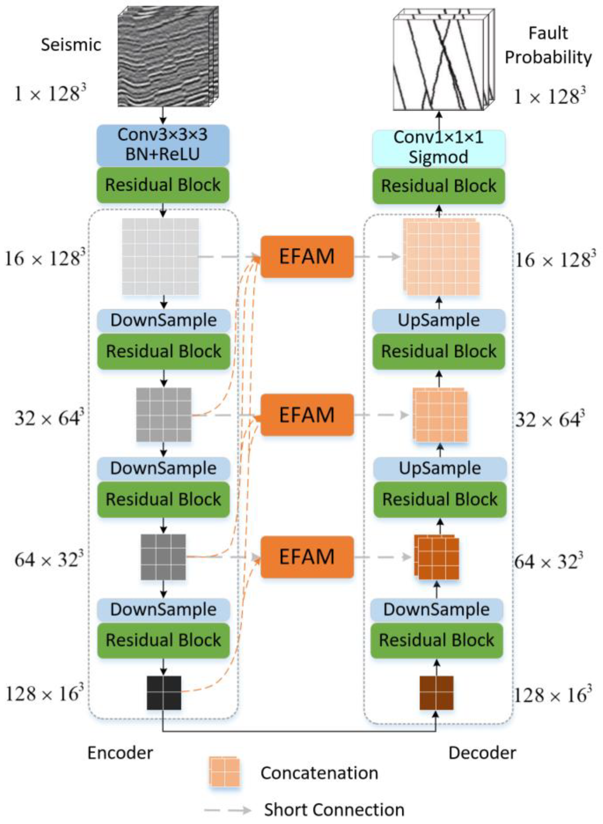
The overall structure of the EAResU-net is shown in Figure 1. The EAResU-net possesses an encoder–decoder architecture, which comprises a contracting path (the encoder on the left) and an expansive path (the decoder on the right). In the U-net, encoder and decoder at the same level are directly connected through skip connections without any modifications. In contrast, in EAResU-net, we propose utilizing attention blocks with enhanced feature fusion to enhance encoder features, followed by connecting each encoder to a decoder at the same level. The attention block with enhanced feature fusion at each level is constructed from the current layer and the encoders and decoders below it after appropriate upsampling and convolution. Another notable feature of EAResU-net is that all encoders and decoders in the contraction and expansion paths are composed of residual convolutional blocks, which replace the ordinary blocks in the original U-net. In contrast to the U-net, the new components in the EAResU-net are inspired by several previous works, such as the residual network [20], Attention Gate mechanism [31], and ExFuse architecture [29]. Our EAResU-net leverages the advantages of these architectures and builds a streamlined architecture.

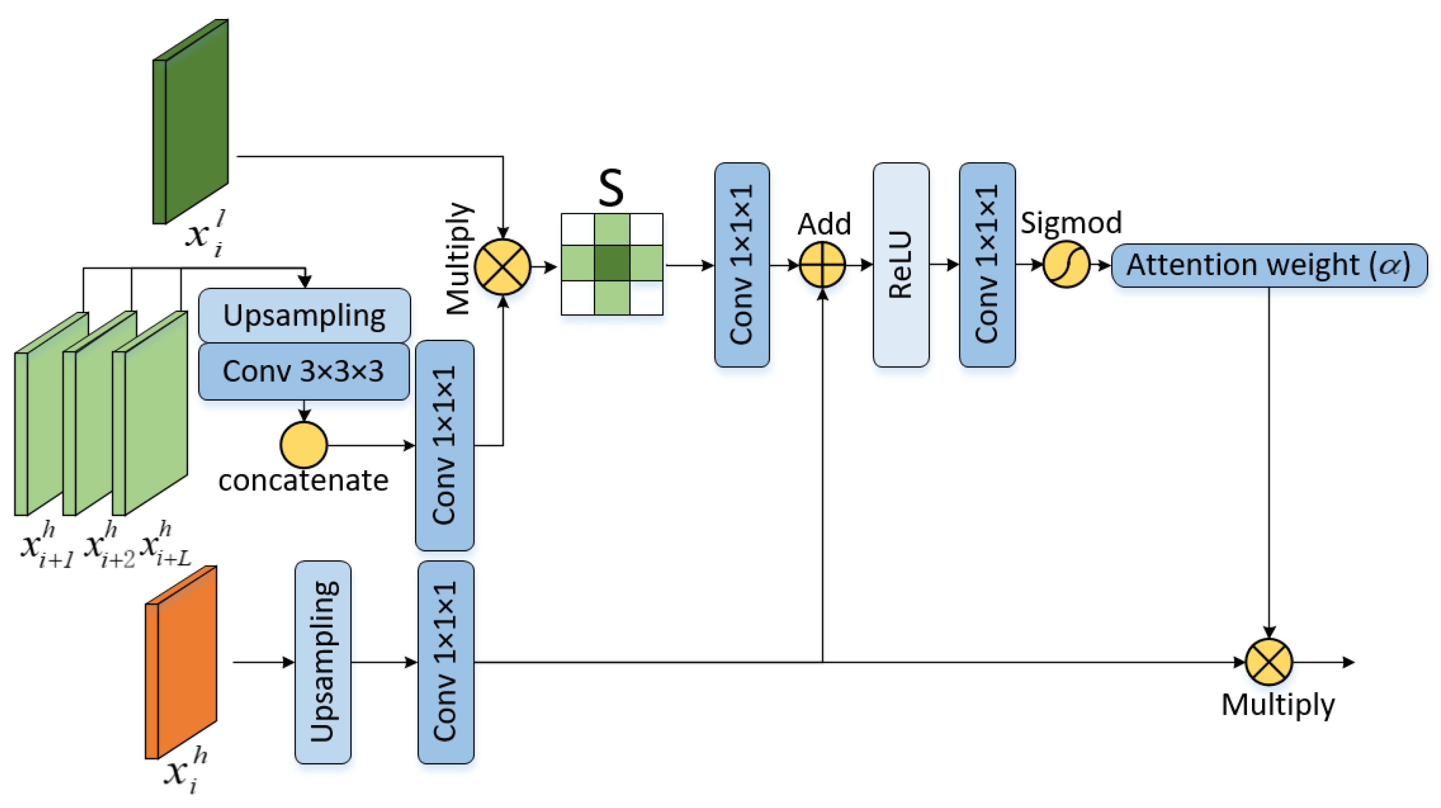
We explain how the attention block for enhanced feature fusion works by using the process of first-layer encoder feature improvement as an example. In the traditional U-Net architecture, the encoder skips connections to the decoder at the same layer without any refinement, thus incorporating only the feature information in the current encoder layer. In EAResU-net, an attention module with enhanced feature fusion (EFAM) is constructed, which improves the encoding process by incorporating rich feature information from the lower-level encoder prior to being skip-connected to the decoder. The architecture of EFAM is illustrated in Figure 2, which comprises two components: the enhanced feature module and the attention module. In the following, we use $x_i$ to represent the feature map and $x_i^h$ and $x_i^l$ to represent the high-level and low-level features, where $i=(\mathrm{1,2},\mathrm{3,4})$ is the number of layers of the encoder.

The purpose of the enhanced feature module is to embed semantic information from deep features into low-level features containing only spatial information, in order to guide the feature fusion between the encoder and decoder. To construct the enhanced feature map $S_1$ of the first layer encoder, we upsampled the feature $x_2^h$ of the second layer encoder using trilinear interpolation with a ratio of 2; we upsampled the feature $x_3^h$ of the third layer encoder using trilinear interpolation with a ratio of 4; and we upsampled the feature $x_4^h$ of the fourth layer encoder using trilinear interpolation with a ratio of 8. For the upsampled features, we performed a convolution operation with a kernel size of (3 × 3 × 3) and concatenate the three feature maps together. The number of feature channels is then compressed by a 1 × 1 × 1 convolution to the same number as the current encoder feature $x_1^l$. Finally, we dot product the compressed features with $x_1^l$ to create the enhanced feature matrix $S_1$. The rationale behind this design is that using upsampling combined with convolutional operations can retrieve high-level semantic information from the higher-level encoder, while dot product means that high-level semantic features are mapped to low-level spatial features in order to guide feature fusion. The process of constructing the enhanced feature module can be expressed as:

$$S_i=x_i^l⨀{\omega }_f^T\sigma \left({\omega }_{\theta }^T{\mathcal{F}}^{cat}\left(x_{i+1}^h,x_{i+2}^h,{\dots ,x}_L^h\right)\right)$$

(1)

where $\sigma$ is the upsampling function, ${\omega }_{\theta }$ is a 3 × 3 × 3 convolution operation, ${\omega }_f$ is a 1 × 1 × 1 linear transformation, the symbol $⨀$ represents the dot product, and ${\mathcal{F}}^{cat}(·)$ represents the feature concatenation.

We also built an attention module that enables the model to focus on fault-related information on the feature maps rather than noise. The module obtains linear projections ${\omega }_s^{T}S$ and ${\omega }_h^T{x}^h$ from low-level features $S$ that fuse semantic information and high-level features $x^h$ at low resolution in the decoder network by 1 × 1 × 1 convolution, respectively. Since fault recognition is a binary classification task, we did not use multidimensional attention coefficients suggested by [31]. Instead, we upsampled the low-resolution features and then combined the two linear projections directly into a single channel by convolution. We expected the attention map to effectively suppress the non-fault region features in $S$ and retain the features in the fault region. So, the final attention weight map $\alpha$ was calculated by the sigmoid function, such that the weight should go from 0 to 1 in line with the decreases in Euclidean distance from the fault area. The whole process is expressed as:

$${\alpha }_i=sigmod\left({\omega }_{\psi }^T{ReLU}^T\left({\omega }_s^T{S}_i+\sigma \left({\omega }_h^T{x}_i^h\right)\right)\right)$$

(2)

where ${\alpha }_i\in \left[0,1\right],\sigma$ is the upsampling function, and $\omega \_\psi ,\omega \_s,$ and ${\omega }_h$ are all 1 × 1 × 1 linear maps. This attention module finally merges the attention map $\alpha$ with the upsampled features $x^h$ in the decoder network using element-by-element multiplication. This design forces the model to learn the location and shape of the salient regions associated with the object segmentation of interest. In contrast to the approach presented in reference [31], our attention mechanism derives an attention graph from fused features, wherein the semantic information embedded within the high-resolution features serves to direct the amalgamation of high-level and low-level features.

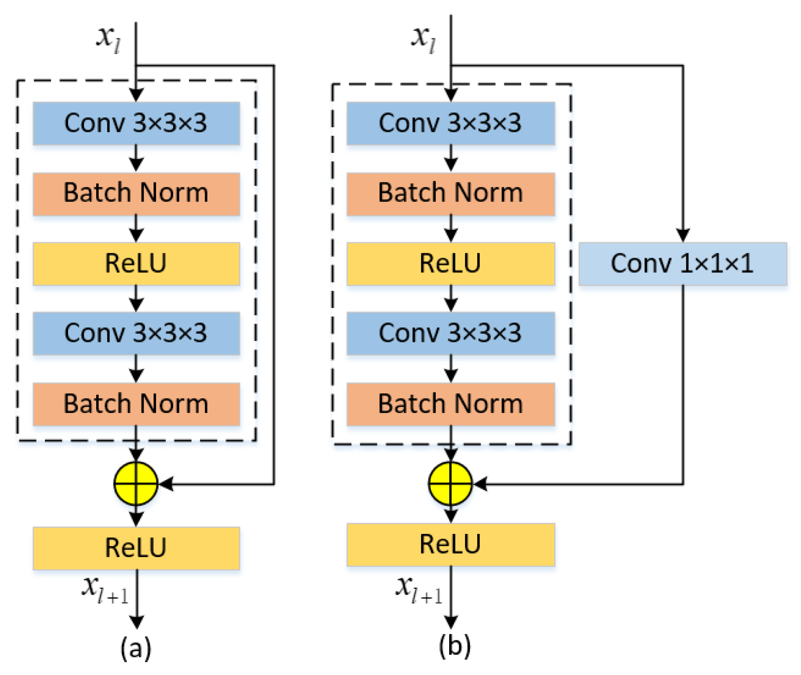
Another important component of EAResU-net is the residual block. In this study, we used the residual block instead of the normal convolution block in the encoder and decoder (Figure 3), which is mathematically represented as:

$$x_{l+1}=x_l+F\left(x_l\right)$$

(3)

where $x_l$ is the constant mapping part and $F\left(x_l\right)$ is the residual mapping part. The input of the residual block is added to the output after two convolutional layers and passed to the next stage. However, when the input and output have different numbers of feature mappings, the input is convolved by 1 × 1 × 1 to match the number of feature mappings with the number of feature mappings of the output (Figure 3b).

In addition, to improve the training speed and accuracy of the model, we added a batch normalization layer before each rectified linear unit (ReLU) activation layer in the neural network. Batch normalization regularizes the data in mini-batch units so that the data conform to a normal distribution with mean $\mu$ of 0 and variance ${\sigma }^2$ of 1. Its mathematical representation is as follows:

$$\mu =\frac{1}{m}\sum _{i=1}^m{x}_i$$

(4)

$${\sigma }^2=\frac{1}{m}\sum _{i=1}^m{\left(x_i-\mu \right)}^2$$

(5)

$$y_i=\gamma \frac{\left(x_i-\mu \right)}{\sqrt{{\sigma }^2+\epsilon }}+\beta$$

(6)

where $x_i$ is the mini-batch data, $y_i$ is the normalized value, $\gamma$ and $\beta$ are the scale and displacement parameters, $\epsilon$ is used to ensure the stability of the normalized value, and $m$ is the size of the input data.

Fault identification is essentially a binary problem. However, there is a clear imbalance between the number of seismic faults and non-faults, with the number of non-faults being much larger. In this case, the classifier is likely to favor the non-fault category with a larger number of samples and ignore the fault category with a smaller number of samples. This can lead to frequent misclassification by the model of few categories of faults as non-fault categories during the prediction process. To solve this problem, we used a smoothed dice loss function [32,33]:

$$L=1-\frac{2{\sum }_{i=1}^N{p}_i{y}_i+1}{{\sum }_{i=1}^N{p}_i+{\sum }_{i=1}^N{y}_i+1}$$

(7)

where $y_i$ is the ground truth label of the $i$th image pixel value, $0\le p_i\le 1$ is the prediction probability of the $i$th image pixel value, and $N$ is the number of samples. The global overlap between the predicted values of the dice loss metric neural network and the ground truth values makes it suitable for training neural networks with imbalanced datasets.

Table 1. Comparison of parameter quantity and execution efficiency of different networks.

Models	Parameters	FLOPs (1283)	Infer Time (1283/GPU)	Infer Time (1283/CPU)
U-net	1.5 M	127.42 G	0.20	2.42
ResU-net	3.7 M	290.11 G	0.31	2.85
EAU-net	2.9 M	214.24 G	0.27	2.64
EAResU-net	4.5 M	291.66 G	0.33	2.92

presents a comparative analysis of the network parameters and computational efficiency between EAResU-net and previous works, namely U-net [12] and ResU-net [13]. The inclusion of EFAM and residual modules in EAResU-net results in a notable increase in computational requirements compared to U-net. However, when compared to ResU-net, EAResU-net exhibits only marginal increments in parameter count and execution time. This indicates that the integration of our EFAM module requires minimal additional allocation of computational resources, and its performance has been empirically demonstrated to be superior to previous works.

3. Experiment

3.1. Experiment Preparation

In the field of 3D fault identification, training neural network models requires a large amount of seismic data and their corresponding fault labels. However, manually labeling faults in real seismic data is a time-consuming and highly subjective task, and the 3D and spatial characteristics of faults increase the difficulty of manual interpretation. This may lead to labeling errors, which may affect the learning and training of neural networks. We, therefore, used synthetic seismic data with fault labels to train our neural network. The synthetic seismic datasets are derived from open-source datasets [17], which are automatically generated by randomly adding folds, faults, and noise to the volumes. The simplified procedure for synthetic seismic data is as follows:

(1) Generate a horizontal reflection model where the reflection coefficients are random in the [−1,1] interval.

(2) Add a stratigraphic fold operation to the horizontal reflection model and carry out a vertical distortion of the strata. The function defining the folding operation is as follows:

$$f_1\left(x,y,z\right)=a_0+\frac{2.0z}{z_{max}}\sum _{k=1}^{k=N}{b}_k{e}^{\frac{{\left(x-c_k\right)}^2+{\left(y-d_k\right)}^2}{{2\sigma }_k^2}}$$

(8)

It combines multiple two-dimensional Gaussian functions and a linear scale function of $2.0z/z_{max}$. The combination of two-dimensional Gaussian functions creates lateral variations in the geological folding structures, while the linear scale function suppresses vertical variations in the geological folding. In the equation, $a_0,b_k,c_k,d_k$, and ${\sigma }_k$ represent different folding parameters. By randomly determining these parameters, models with varying folding structures can be generated.

(3) Add a random number of faults with random dip and spatial location to the model. It is expressed as:

$$r_1\left(x,y,z\right)=r\left(x,y,z+f_1+f_2\right)e^{-\frac{1}{2}{z}^T{R}^T{S}^{T}Rz}$$

(9)

In the equation, $r\left(x,y,z+f_1+f_2\right)$ represents a horizontally reflected model with different geological folding, where $R$ is a one-dimensional vector composed of $\mu f$ (fault dip vector), $\nu f$ (fault strike vector), and $\omega f$ (fault normal vector), and $S$ represents a diagonal matrix composed of elements from vector $R$.

(4) Fold Ricker subwaves with the reflection model to obtain a 3D seismic record.

(5) Add random levels of noise to the seismic record.

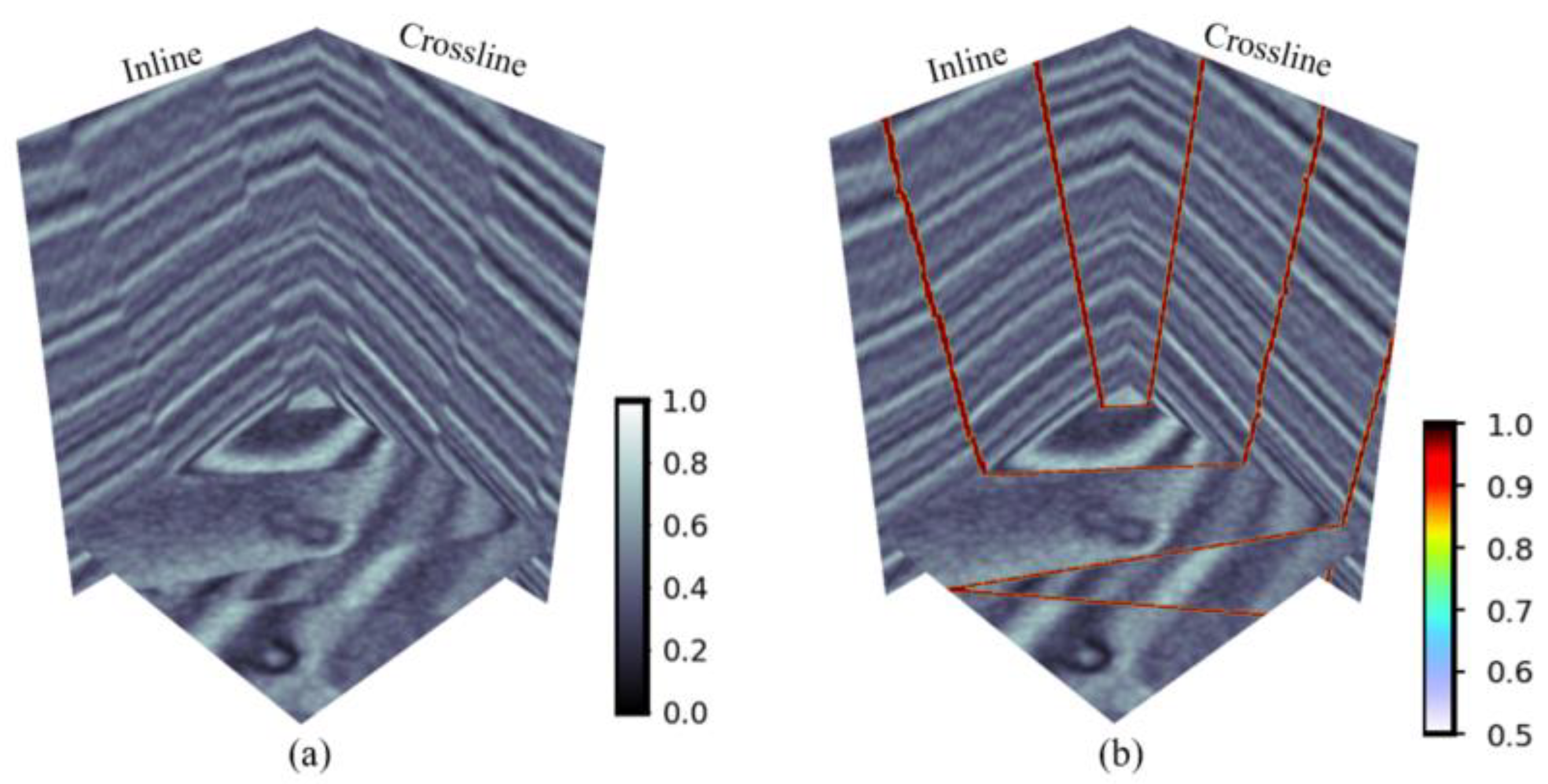
We employed this methodology to generate a training dataset of 200 pairs of 128 × 128 × 128 volumetric data, and a validation dataset of 20 pairs of the same size. Figure 4 presents the three-dimensional visualization results of the synthetic seismic data and fault labels. To increase the diversity of the model training, we performed random horizontal and vertical flipping of the training data.

The experimental code was implemented by Pytorch 1.11.0 and trained by Apex acceleration. The optimizer used AdamW [34] with an initial learning rate of 0.001 and a batch size of 4. As the number of iterations increases, the learning rate decays to avoid network oscillations and prevent overfitting. The model was initialized using the kaiming method [35]. Each experiment was trained for 200 epochs and run once per period on the validation set to record quantitative metrics. All computations were performed on a server equipped with RTX A5000 (24G GPU memory).

3.2. Evaluation Metrics

In order to assess the accuracy of the model, we employed various commonly utilized evaluation metrics, namely Intersection over Union (IOU), Dice Similarity Coefficient (DSC), recall (Rec), precision, and F1-score.

The IOU represents the similarity between the predicted and ground truth regions, which is expressed as:

$$\mathrm{I}\mathrm{O}\mathrm{U}=\frac{\mathrm{T}\mathrm{P}}{\mathrm{F}\mathrm{P}+\mathrm{T}\mathrm{P}+\mathrm{F}\mathrm{N}}$$

(10)

Among them, true positive (TP) indicates that the actual positive sample is also predicted to be positive. False positive (FP) indicates that the actual sample is negative but predicted to be positive. False negative (FN) means that the actual sample is positive but predicted to be negative. The model calculates IOU by sigmod activation function normalizing the output to probability $y_i\in \left[\mathrm{0,1}\right]$ and considering $y_i>0.5$ as a positive sample and $y_i<0.5$ as a negative sample.

DSC is an ensemble similarity measure function that is usually used to calculate the similarity of two samples and is expressed similarly to IOU:

$$\mathrm{D}\mathrm{i}\mathrm{c}\mathrm{e}=\frac{2\mathrm{T}\mathrm{P}}{\mathrm{F}\mathrm{P}+2\mathrm{T}\mathrm{P}+\mathrm{F}\mathrm{N}}$$

(11)

The recall rate, R, indicates the proportion of correctly predicted positive samples to all positive samples. The recall rate is expressed as:

$$\mathrm{R}=\frac{\mathrm{T}\mathrm{P}}{\mathrm{T}\mathrm{P}+\mathrm{F}\mathrm{N}}$$

(12)

The precision, P, represents the proportion of samples that are predicted to be positive and are actually positive to all samples that are predicted to be positive. The larger the P value, the better the prediction, as defined below:

$$\mathrm{P}=\frac{\mathrm{T}\mathrm{P}}{\mathrm{T}\mathrm{P}+\mathrm{F}\mathrm{P}}$$

(13)

F1-score is the summed average of precision and recall, which takes into account both precision and recall. F1-score is defined as:

$$\mathrm{F}1=\frac{2\times \mathrm{P}\times \mathrm{R}}{\mathrm{P}+\mathrm{R}}$$

(14)

3.3. Experimental Results and Analysis

To validate the effectiveness of the proposed model, we trained four network models using a synthetic 200-pair training dataset with the same hyperparameters: (1) the conventional U-net used by Wu et al. [17]; (2) the ResU-net with residual structure introduced in the U-net by Liu et al. [19]; (3) the EAU-net embedded with our EFAM in the U-net; and (4) our proposed EAResU-net. We applied the four models to a 20-pair validation dataset and quantitatively evaluated the fault prediction results.

The model with the maximum IOU on the validation set was saved as the final model, and we performed quantitative analysis on the predicted fault results of the four models. The quantitative evaluation is shown in

Table 2. Validation set model performance comparison.

Models	IOU	Dice	Recall	Precision	F1 Score
U-net	0.6569	0.7919	0.7194	0.9866	0.8316
ResU-net	0.6910	0.8163	0.7515	0.9886	0.8535
EAU-net	0.6720	0.8028	0.7337	0.9876	0.8415
EAResU-net	0.7036	0.8251	0.7704	0.9885	0.8656

, and we noted that our EAResU-net outperforms the other three models in many aspects, with more significant improvement compared to U-net. Although ResU-net performs similarly to our model in terms of accuracy, its lower recall indicates that it misses many fault structures and produces a significant number of false negatives (FP) in its predictions. Furthermore, the traditional U-net model has shown a significant improvement after the introduction of EFAM. This indicates the effectiveness of our proposed EFAM in enhancing the feature fusion and fault attention of the U-net network. It is worth noting that compared to ResU-net and EAResU-net, EAU-net has shown mediocre results. We speculate that this is due to the fact that EAU-net employs ordinary convolutional layers for feature extraction, which have relatively weak feature extraction capabilities, thus failing to capture more effective fault features.

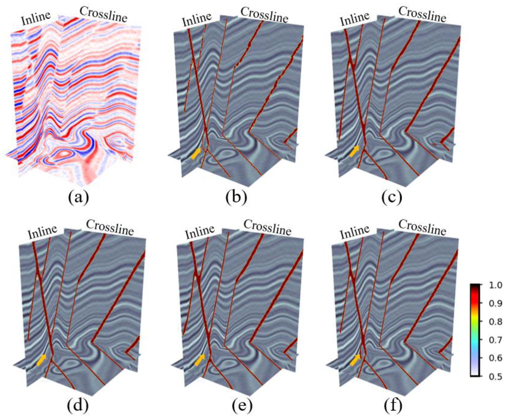
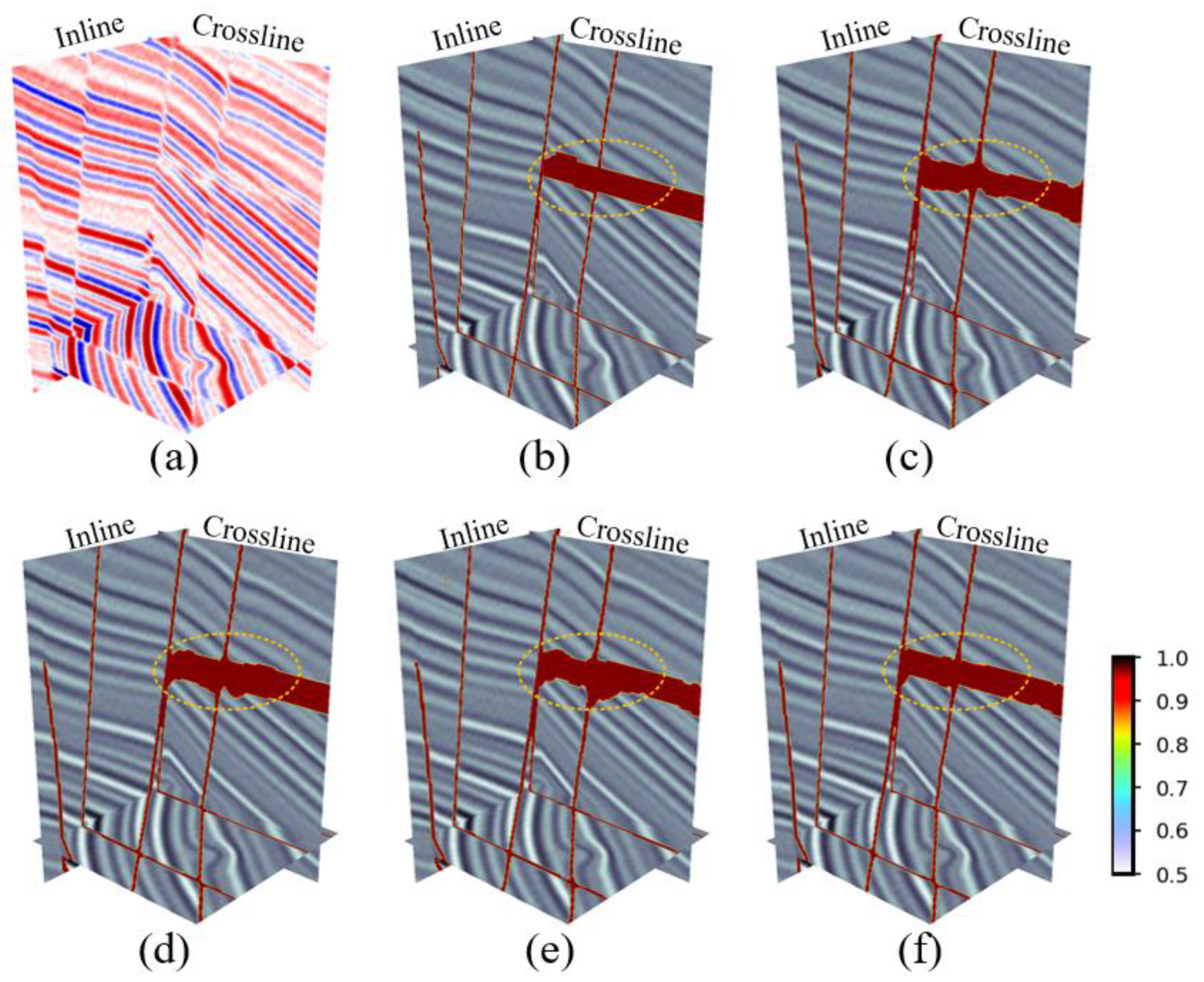
In addition, a qualitative evaluation of the proposed model was conducted through the visualization of the results of fault prediction using two validation datasets. Figure 5 and Figure 6 illustrate the raw seismic data slices of the validation datasets along with the true labels and predicted results of the fault segmentation.

As shown in Figure 5 and Figure 6, all four networks capture the features of the faults to identify the location of the faults and predict the shape and distribution of the faults to be consistent with the actual fault labels. Compared with EAResU-net, none of the remaining three networks can identify the small faults at the yellow arrows in Figure 5, and for the fault zones (marked in yellow in Figure 6), our predictions are closer to the true label. This highlights the advantages of the method proposed by us, where EFAM enhances the identification of minor faults and significantly improves the accuracy of fault identification.

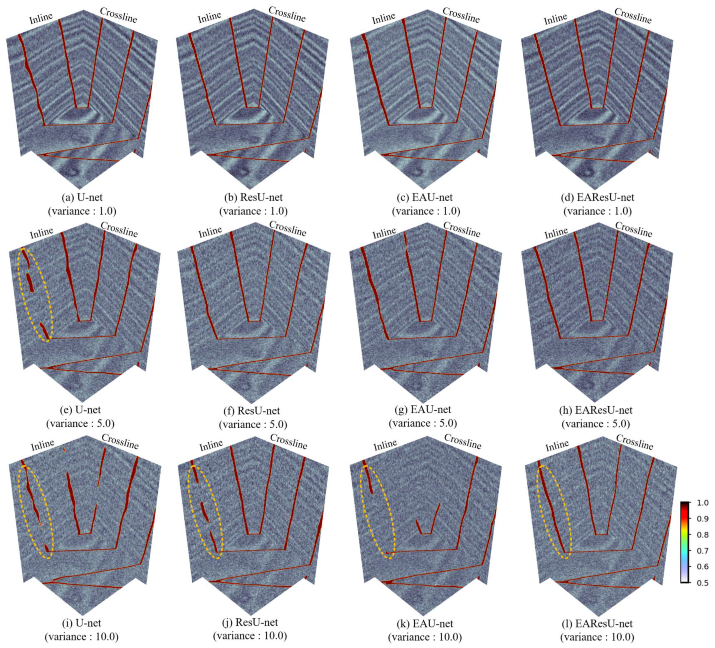
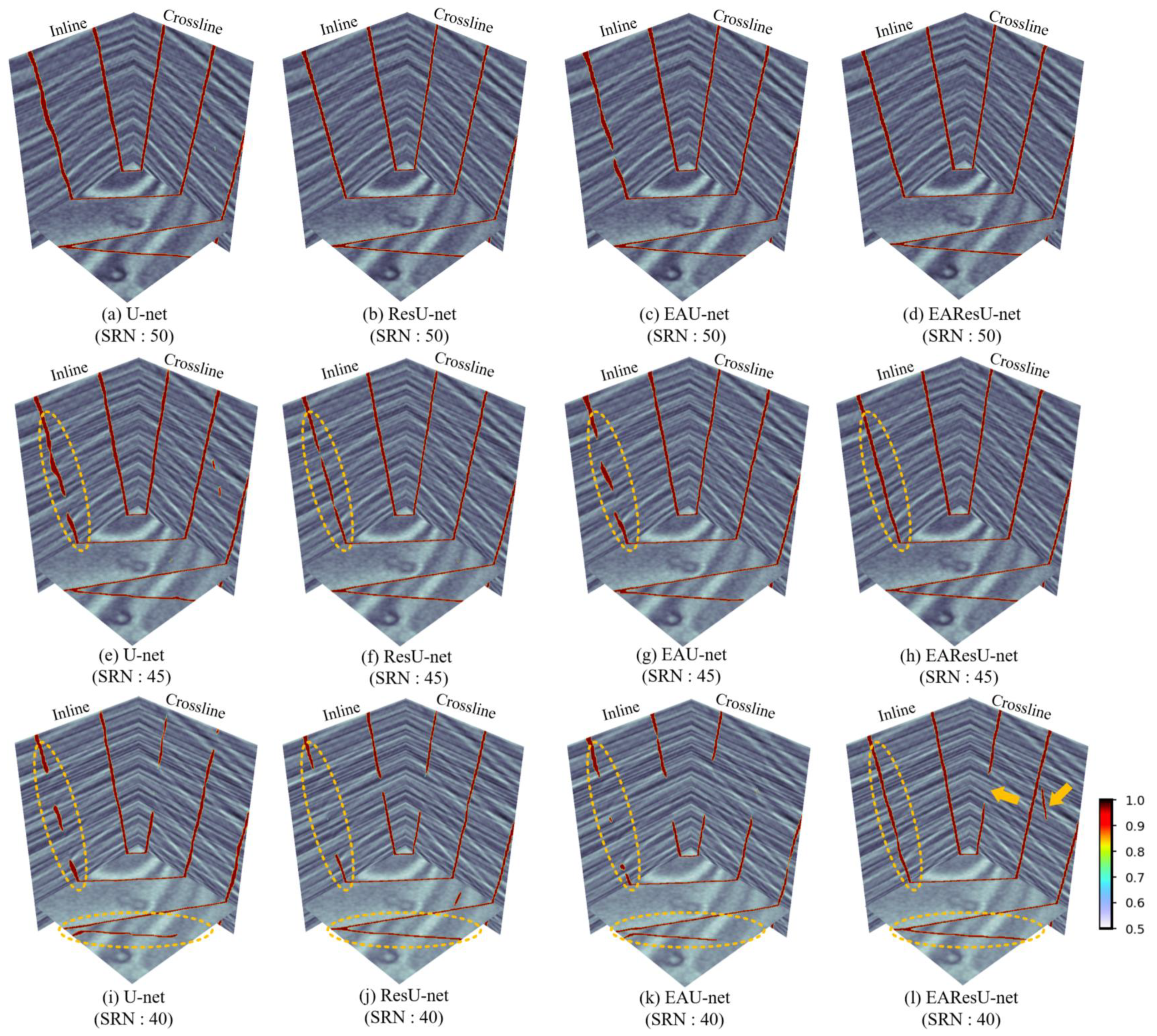
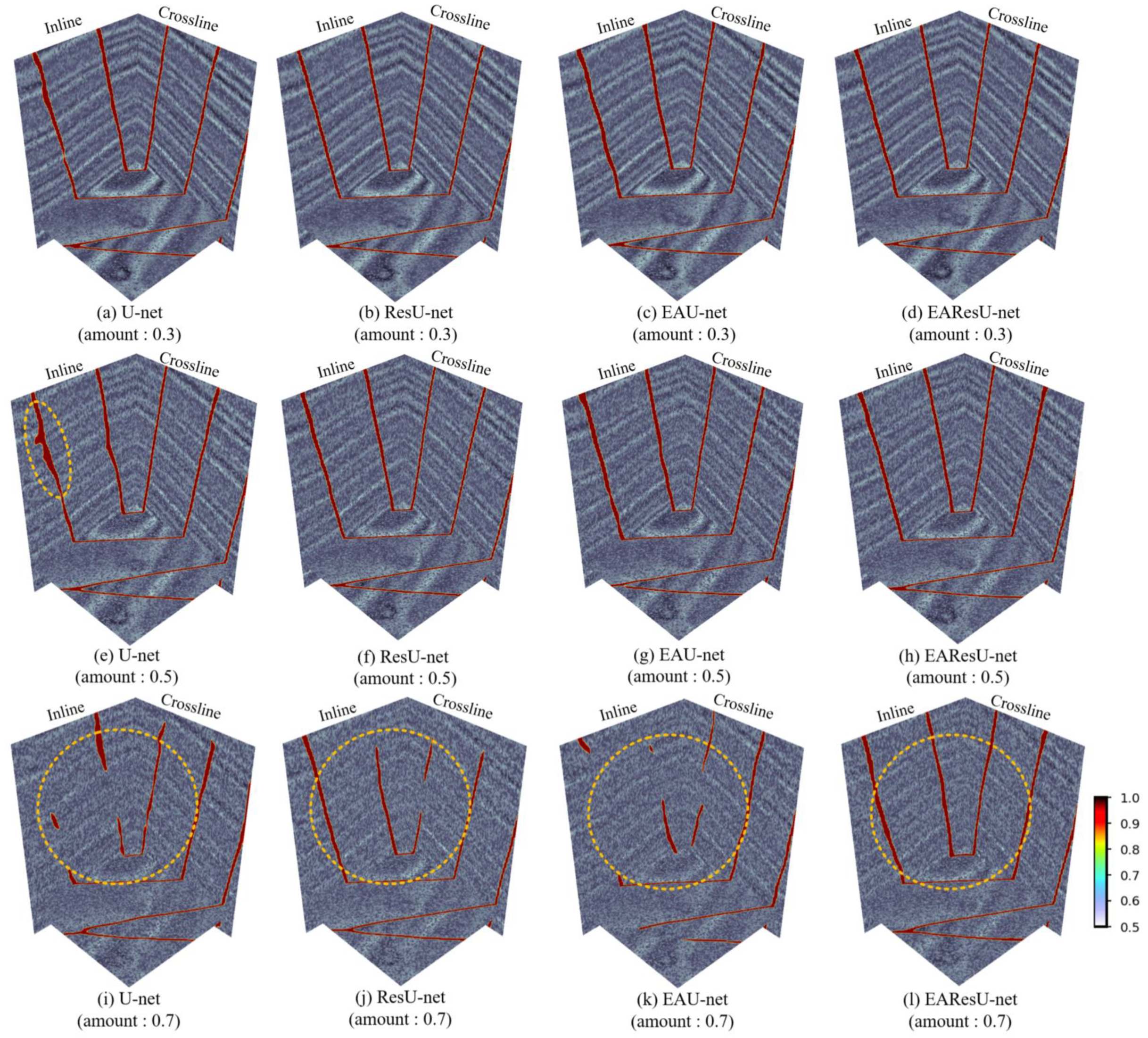
To further validate the robustness of the proposed model to different levels of seismic data noise, we added varying degrees of Gaussian noise, white noise, and salt-and-pepper noise to synthetic data (Figure 4).

Table 3. Types of noise and their respective noise level parameters.

Noise Type	Low Level	Middle Level	High Level
Gaussian noise	Variance/1.0	Variance/5.0	Variance/10.0
White noise	SRN/50	SRN/45	SRN/40
Salt-and-pepper noise	Amount/0.3	Amount/0.5	Amount/0.7

displays the types of added noise and their respective noise level parameters, where Gaussian noise is measured by variance, white noise is measured by Signal-to-Noise Ratio (SNR), and salt-and-pepper noise is measured by the amount parameter ranging from 0 to 1. Figure 7, Figure 8 and Figure 9 illustrate the fault results of the four models predicting seismic data with varying levels of noise.

In Figure 7, Figure 8 and Figure 9, all four models can effectively identify faults in seismic data with low-level noise [(a), (b), (c), and (d) in Figure 7, Figure 8 and Figure 9]. However, as the noise level increases, the prediction results of U-net are slightly affected by the noise in the seismic data with Gaussian noise of variance 5.0 [Figure 7e] and salt-and-pepper noise with an amount of 0.5 [Figure 9e]. Additionally, in Figure 8, for white noise seismic data with an SNR of 45, U-net [Figure 8e], ResU-net [Figure 8f], and EAU-net [Figure 8g] show discontinuous fault lines in their predictions. In contrast, for seismic data with moderate-level noise, our EAResU-net can accurately identify faults completely [(h) in Figure 7, Figure 8 and Figure 9]. As the noise level increases to a high level, the prediction outcomes of the three comparative models exhibit a significant loss of fault information [(i), (j), and (k) in Figure 7, Figure 8 and Figure 9]. For white noise seismic data with an SNR of 40 (Figure 8), the predictions of EAResU-net [Figure 8l] are partially affected by the noise, resulting in intermittent faults and false faults. However, in the remaining two types of noisy data, the fault identification results of EAResU-net [Figure 7l and Figure 9l] exhibit higher accuracy and completeness compared to the fault identification results of the other three models. Overall, our EAResU-net demonstrates significant advantages in suppressing different levels of seismic data noise and exhibits good robustness to high-level noise in seismic data.

3.4. Testing Field Data

After training and validating the models, we applied them to 3D field data from different surveys to compare the performance of these methods on publicly available data.

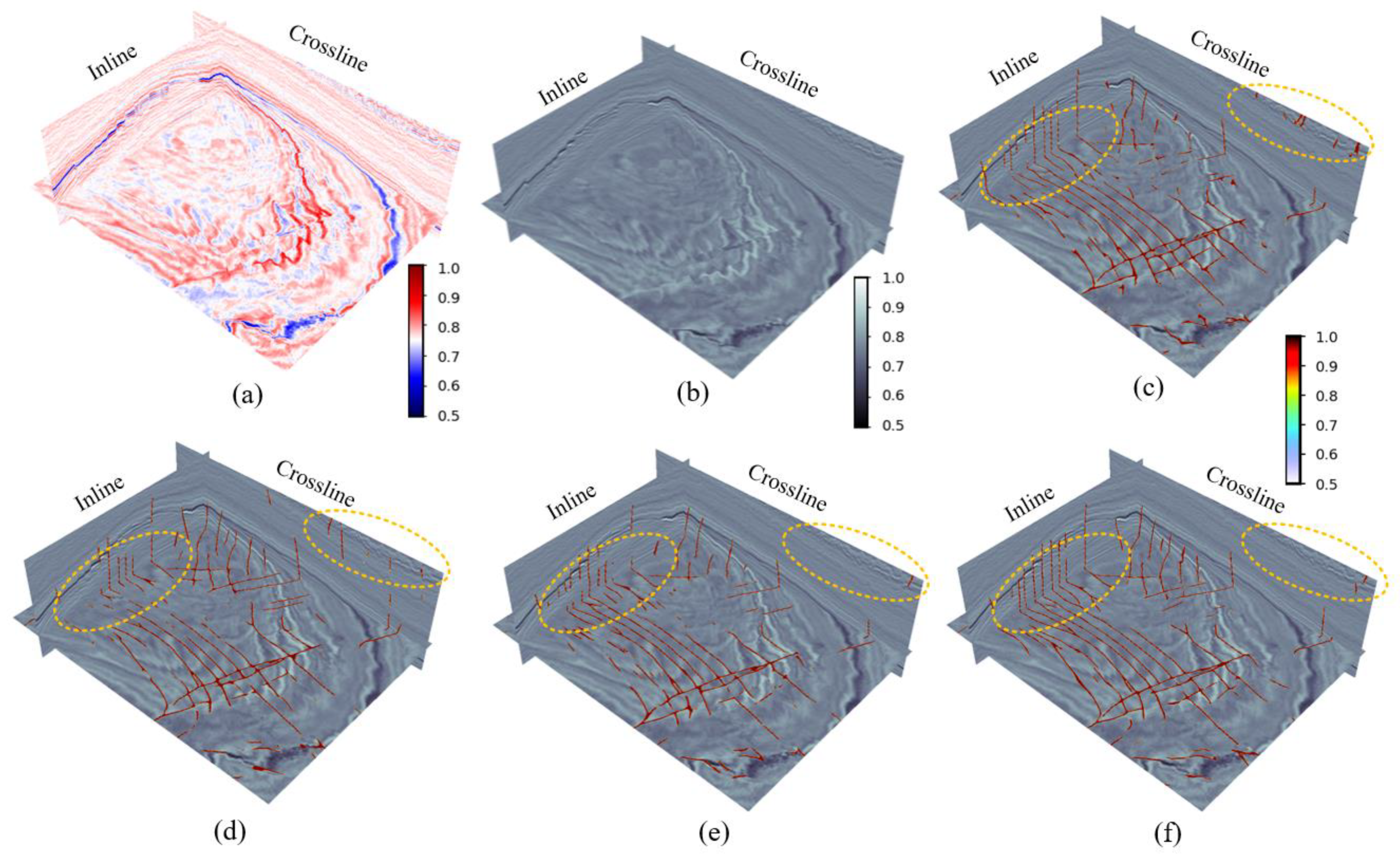
(1) Netherlands F3: We conducted a test on the seismic data of the Netherlands F3 block provided by the Dutch government using dGB Earth Sciences. We selected a region with a more complex fault system, which contains some intersecting faults. The selected region comprises 128 × 512 × 384 grid points.

Figure 10 presents a three-dimensional display of seismic data and fault prediction results in the F3 working area. In Figure 10, all four models can identify faults well, but our model (d) characterizes faults more completely and continuously (circled on the left side of Figure 10). Among them, the fault lines extracted by U-net (b) are discontinuous. Although ResU-net (c) predicts more complete faults than those extracted by U-net, there are still a few discontinuous fault lines. Both EAU-net (d) and EAResU-net (e) exhibit robustness to seismic noise (circled on the right side of Figure 10), but due to the EAResU-net model’s use of residual convolution as the basis, its fault structure is more complex and fault lines are more complete than EAU-net (d). This verifies the effectiveness of our model and the significant advantage of EFAM in enhancing model performance and suppressing seismic noise.

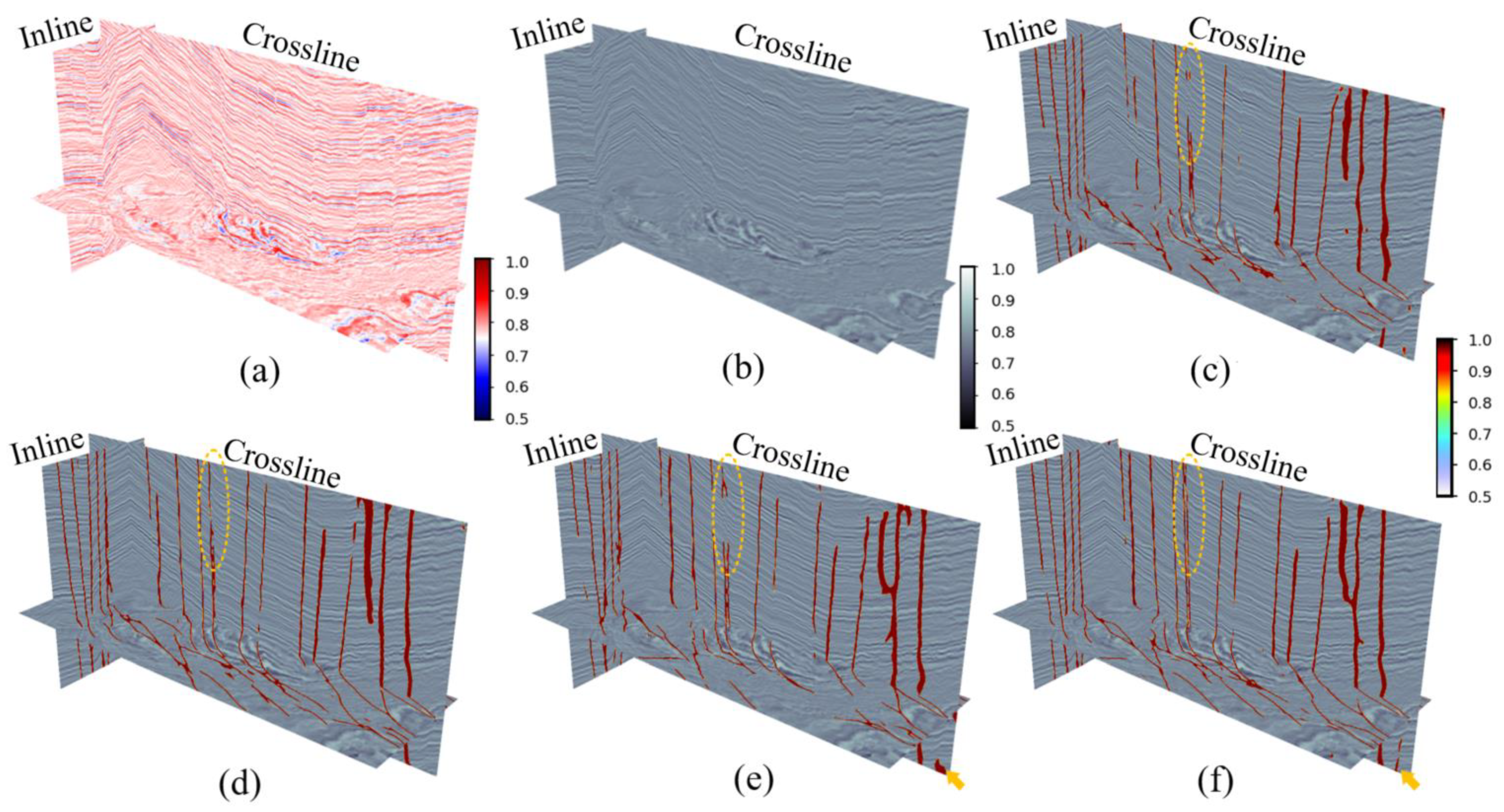
(2) New Zealand Kerry-3D: This data is the final volume of field data for the pre-stack offset provided by Crown Minerals of New Zealand. We intercepted the fault-rich area of it, and the size of the sampled area was 192 × 608 × 224.

Figure 11 illustrates the truncated testing data and experimental results. It is evident that the Kerry-3D field data contain seismic faults of different scales, with a predominance of vertical faults, which are more pronounced on reflective surfaces. Figure 11b presents the fault prediction results obtained by U-net, which show a clear distribution of faults but poor continuity of small and irregular faults, making them difficult to identify. In comparison, the predicted fault results by ResU-net in (c) are more complete, with improved fault continuity, but exhibit noisy fault features and poor identification of minor faults. The fault prediction results by EAU-net in (d) demonstrate reduced omission of small faults and errors due to noise compared to U-net, but the completeness of faults is inferior to ResU-net in (c). In contrast, the fault boundaries predicted by EAResU-net in (e) are clear, and the representation of intricate fault details and adjacent faults is complete, with minimal noise in fault features, enabling accurate identification of small faults (highlighted in yellow in Figure 11).

In conclusion, the fault recognition method proposed by our EAResU-net exhibits high accuracy in fault recognition, effectively suppresses noise, and enhances the recognition of minor faults and fault details.

4. Conclusions

We proposed a novel fault recognition method using EAResU-net, which utilizes attention modules with enhanced feature fusion, residual convolution, and smooth dice loss function to improve automatic fault detection capability. Our neural network was trained on 3D synthetic seismic data and then compared with state-of-the-art U-net and ResU-net models. The experimental results on synthetic datasets and two field datasets demonstrate that our EAResU-net can capture richer fault features and is highly noise-proof for providing clear fault detection results, even in complex seismic structures.

Nevertheless, our approach still has some limitations. Firstly, we trained our CNN model solely on synthetic seismic data without the need for any manual annotations. While the trained model performs well on different field data, there is a significant drawback to using synthetic data. Deep learning models require a large amount of data, and the limited synthetic dataset cannot guarantee stable generalization of the trained model under all geological conditions of faults. Secondly, although our model can effectively suppress noise in seismic data, it does not exhibit strong robustness to high levels of seismic data noise. This limitation means that the well-trained model may not be fully applicable to the task of fault interpretation in complex field seismic data under high noise conditions. Therefore, combining real seismic data for training the CNN model and improving the model’s stability under high noise levels are the main directions for our future work. Additionally, seismic fault interpretation is just one typical semantic segmentation problem in seismic interpretation. Hence, the proposed model can easily be extended to address other semantic segmentation tasks in seismic interpretation, such as facies analysis and horizon interpretation. This opens up new possibilities for researchers studying other seismic interpretation tasks.