A Backprojection-Based Autofocus Imaging Method for Circular Synthetic Aperture Radar

Abstract

Circular synthetic aperture radar (CSAR) can obtain higher image resolution and more target information through 360° observation of the target. However, CSAR is often subject to motion errors due to the sensor’s accuracy limitations and the unique trajectory of the system. The autofocusing back projection algorithm based on the optimization of image sharpness compensates for motion errors through phase-error estimation. This method can attain relatively good performance while assuming the same error for all pixels; it ignores the spatial variance of motion errors. In order to solve this problem, this paper proposes an autofocusing method based on the Prewitt operator and particle swarm optimization (PSO), which first extracts the subaperture image feature points as a new dataset using the Prewitt operator, estimates the radar slope error on the new dataset using PSO, and subsequently compensates the subaperture image. Finally, the subaperture images are synthesized using an image-alignment method. The results of both the simulated experiments and the measured data validate the effectiveness of this method.

1. Introduction

CSAR is an advanced imaging technique that enables a 360° observation of the target [1]. During the imaging process, the platform moves along a circular trajectory and the antenna beam is continuously pointed at the observation scene. Compared to linear SAR (LSAR), CSAR provides more dimensional information about the scene target and, therefore, CSAR contains a broader prospect for practical applications [2].

The fundamental prerequisite for CSAR to be widely used is the acquisition of high-resolution, high-quality microwave images. SAR-imaging algorithms are divided into two main categories: time-domain and frequency-domain imaging algorithms. The most widely used frequency-domain imaging algorithms are distance Doppler (RD) [3], beam domain (omega-K, $\omega k$) [4], and Chisp scaling (CS) algorithms [5]. All frequency-domain algorithms require a fast Fourier transform for fast imaging purposes, but to take advantage of the FFT, a polynomial approximation to the echo model has to be made. The most typical time-domain algorithm is the back-projection (BP) algorithm, which is distinguished by the fact that no approximations are made and theoretically accurate imaging can be achieved [6]. However, in practice, shaking and vibration of the carrier platform, as well as wind and turbulence, can cause nonlinear antenna phase center (APC) shifts, which can seriously affect the performance of the BP algorithm. Therefore, to obtain high-resolution CSAR imaging results, the issue of motion compensation must be considered.

The most common method of motion compensation is based on the fusion of position information from the inertial measurement unit (IMU) and global positioning system (GPS). However, due to the unstable platform motion, the low accuracy of the position measurement system, APC, and inertial guidance system position information being out of sync, CSAR data after motion compensation always has significant residual position errors to be rectified. To deal with motion errors in the experimental CSAR data processing, several autofocus approaches employing setup calibrators have been proposed. Dungan and Nehra present an algorithm that uses quad-trihedrals resettled in the illuminated scene to generate global range-focusing parameters and phase [7,8].

In the airborne CSAR experiment carried out by ONERA, deterministic triangulation is used to retrieve the trajectory [9]. Nevertheless, this method requires several setup calibrators whose positions are preknown. Chen proposed an autofocus method for CSAR, which could be used in the absence of setup calibrators [10]. However, this method did not consider the effect of space-variant motion error.

There are still no scholars who have achieved precise correction of the spatial variance error of the APC for circular SAR. To address this issue, this paper proposes a motion-compensation method applicable to CSAR. Firstly, feature extraction is performed on the BP image using the Prewitt operator [11]. Based on the optimal intensity criterion, the PSO algorithm is used to estimate the three-dimensional motion error of APC [12]. Finally, the subaperture images are registered and synthesized using an image registration method.

The content of this paper is arranged as follows. Section 2 summarizes the imaging and space-variant error model of CSAR, analyzes the spatial variance characteristics of motion errors, and discusses the shortcomings of the ABP (autofocus backprojection) algorithm [13]. Section 3 introduces the algorithm in detail. Section 4 verifies the effectiveness of the algorithm through simulation data and actual measurement data.

2. CSAR Imaging and Error Models

The imaging geometry of the circular SAR is shown in Figure 1. The radar carrier moves around the center of the scene in a circle of radius R at height h. The direction of the antenna beam is always directed towards the center of the scene, $\varphi \in \left[0,2\pi \right]$, and represents the angle of the radar carrier in the positive direction of the X-axis. The coordinates of the radar carrier can be obtained from the diagram as $(R\cos \phi ,R\sin \phi ,h)$. In Figure 1, point P is a point target located in the plane of observation with coordinates. Therefore, the instantaneous distance between the radar carrier and the target P is $R\left(\phi ,r_P\right)$. Blue dashed lines represents the direction of beam propagation.

$$R\left(\phi ,r_P\right)={\left(R cos\phi -x_{\mathrm{p}}\right)}^2+{\left(R sin\phi -y_p\right)}^2+{\left(\mathrm{h} -z_p\right)}^2$$

(1)

Assume the transmit signal of the SAR system to be a series of linear frequency modulation (LFM) pulses

$${\mathrm{s}}_T(\mathrm{t})={\displaystyle \sum _{\mathrm{n}=1}^N{\mathrm{s}}_{\mathrm{pul}}(\mathrm{t}-\mathrm{nT})}$$

(2)

where t is the full time, N is the total number of pulses contained in the transmit signal, T is the pulse repetition period, and the linear FM signal of a signal pulse is [14]

$${\mathrm{s}}_{\mathrm{pul}} \left(\tau \right)= \mathrm{rect}\left\{\frac{\tau }{T_p}\right\}\exp \{j2\pi f_c\tau +j\pi K{\tau }^2\}$$

(3)

where rect(·) denotes the rectangular window function, $\tau$ is the fast time variable, $T_p$ is the pulse width of the transmit signal, the $f_c$ is the center frequency of the transmit signal, and K is the linear tuning frequency.

After the transmitted signal is reflected by any point target P in the observation scene, the point target echo signal returned to the receiving antenna is [15]

$${\mathrm{s}}_{\mathrm{pul}} \left(t;{\overrightarrow{r}}_p\right)={\sigma }_p\left(t;{\overrightarrow{r}}_p\right)w_p\left(t;{\overrightarrow{r}}_p\right){\displaystyle \sum _{n=1}^N{s}_{pul}}(t-nT-2R(\overrightarrow{l}(t),{\overrightarrow{r}}_p)/c)$$

(4)

The above equation ${\sigma }_p\left(t;{\overrightarrow{r}}_p\right)$ represents the backscattering coefficients of the target P; $w_p\left(t;{\overrightarrow{r}}_p\right)$ is the antenna modulation factor; and c is the speed of light. After substituting Equation (2) into Equation (3), we get [16]

$$\begin{array}{l}{\mathrm{s}}_{\mathrm{r}} \left(t;{\overrightarrow{r}}_p\right)={\sigma }_p\left(\overrightarrow{l}(t);{\overrightarrow{r}}_p\right)w_p\left(\overrightarrow{l}(t);{\overrightarrow{r}}_p\right){\displaystyle \sum _1^{N}rect[\frac{(t-nT-2R(\overrightarrow{l}(t),{\overrightarrow{r}}_p)/c)}{T_p}]}\\ \hspace{1em}\hspace{1em}\hspace{1em}\hspace{1em}\hspace{1em}\times \exp [j2\pi fc(t-nT-2R(\overrightarrow{l}(t),{\overrightarrow{r}}_p)/c)]\\ \hspace{1em}\hspace{1em}\hspace{1em}\hspace{1em}\hspace{1em}\times \exp [j\pi K(t-nT-2R(\overrightarrow{l}(t),{\overrightarrow{r}}_p)/c{)}^2]\end{array}$$

(5)

CSAR is also based on the “go-stop-go” assumption, that is, because the speed of antenna movements is much smaller than the speed of electromagnetic waves, so the signal in a pulse time in the process of transmitting to be received, ignoring the change in antenna position, it will be considered to remain stationary.

The slow time can be used as the time quantity to describe the antenna motion, and the relationship between the fast and slow time is:

$$t=nT+\eta$$

(6)

In Equation (4), ${\sigma }_p\left(\overrightarrow{l}(t);{\overrightarrow{r}}_p\right)$, $w_p\left(\overrightarrow{l}(t);{\overrightarrow{r}}_p\right)$ are influenced by the relative position between the target and the antenna. According to the above assumptions where the fast time variable can be neglected, that is ${\sigma }_p\left(\overrightarrow{l}(t);{\overrightarrow{r}}_p\right)\approx {\sigma }_p\left(\overrightarrow{l}(\eta );{\overrightarrow{r}}_p\right),w_p\left(\overrightarrow{l}(t);{\overrightarrow{r}}_p\right)\approx w_p\left(\overrightarrow{l}(\eta );{\overrightarrow{r}}_p\right)$. Substituting Equation (5) into (4), the echo signal can be represented by the two dependent variables of fast time $\tau$ and slow time $\eta$.

$$\begin{array}{l}{\mathrm{s}}_{\mathrm{r}} \left(t;{\overrightarrow{r}}_p\right)={\sigma }_p\left(\overrightarrow{l}(\eta );{\overrightarrow{r}}_p\right)w_p\left(\overrightarrow{l}(\eta );{\overrightarrow{r}}_p\right){\displaystyle \sum _1^{N}rect[\frac{(\tau -nT-2R(\overrightarrow{l}(\eta ),{\overrightarrow{r}}_p)/c)}{T_p}]}\\ \hspace{1em}\hspace{1em}\hspace{1em}\hspace{1em}\hspace{1em}\times \exp [j2\pi fc(\tau -nT-2R(\overrightarrow{l}(\eta ),{\overrightarrow{r}}_p)/c)]\\ \hspace{1em}\hspace{1em}\hspace{1em}\hspace{1em}\hspace{1em}\times \exp [j\pi K{(\tau -nT-2R(\overrightarrow{l}(\eta ),{\overrightarrow{r}}_p)/c)}^2]\end{array}$$

(7)

After orthogonal demodulation, the point target echo recorded by the system becomes

$$\begin{array}{l}{\mathrm{s}}_{\mathrm{r}} \left(t;{\overrightarrow{r}}_p\right)={\sigma }_p\left(\eta ;{\overrightarrow{r}}_p\right)w_p\left(\eta ;{\overrightarrow{r}}_p\right)rect[\frac{(\tau -2R(\overrightarrow{l}(\eta ),{\overrightarrow{r}}_p)/c)}{T_p}]\\ \hspace{1em}\hspace{1em}\hspace{1em}\hspace{1em}\hspace{1em}\times \exp [-j4\pi f_{c}R(\overrightarrow{l}(\eta ),{\overrightarrow{r}}_p)/c]\\ \hspace{1em}\hspace{1em}\hspace{1em}\hspace{1em}\hspace{1em}\times \exp [j\pi K{(\tau -2R(\overrightarrow{l}(\eta ),{\overrightarrow{r}}_p)/c)}^2]\end{array}$$

(8)

Equation (8) is the mathematical model of the point target echo signal under CSAR.

The target in the actual scene can be regarded as composed of multiple point targets, so the echo signal received by the radar is composed of the accumulated of all point target echo signals in the irradiated scene, so the expression of the total echo signal is

$$s(\eta ,\tau )={\displaystyle \underset{\left|{\overrightarrow{r}}_p\right|}{\int }{s}_r}(\eta ,\tau ;{\overrightarrow{r}}_p)d{\overrightarrow{r}}_p$$

(9)

This is the BP method for integrating along a circular synthetic aperture for CSAR images; if the backward projection value of the mth pixel point in the imaging space at the kth slow moment is denoted as ${\tilde{b}}_{m,k}$, then the complex image value of the mth pixel is

$$z_m={\displaystyle \sum _{k=1}^K{\tilde{b}}_{m,k}}$$

(10)

According to the ABP algorithm, the final estimated phase error is in fact

$$\phi =[{\phi }_1,{\phi }_2,....{\phi }_k]$$

(11)

where ${\phi }_k$ represents the phase error at the kth slow moment. If the phase error estimated by the ABP is accurately compensated for, the compensated imaging result is

$$z_m={\displaystyle \sum _{k=1}^K{\tilde{b}}_{m,k}}{e}^{-j{\phi }_k}$$

(12)

From Equation (11), it can be seen that the ABP algorithm assumes that each pixel has the same phase error and ignores the spatial variability of motion error. This assumption reduces the complexity of the problem in the computation process but it also reduces the accuracy of image autofocusing.

The motion-compensation method for wide-beam linear SAR, as typically utilized, uniformly compensates the echo data within the range-Doppler domain, with sole consideration for the azimuth spatial phase error. Meanwhile, the traditional large-swath SAR motion-compensation method solely considers the range spatial error, failing to consider the motion error arising from changes in azimuth Doppler angle. It is abundantly clear that neither of these methods is remotely suitable for the circular SAR model.

Given the limitation of the methods, it becomes necessary to explore the impact of range and azimuth slope errors on the CSAR imaging results, all while considering the motion characteristics of the CSAR. It is only through such an understanding that one can truly grasp the intricacies and nuances involved in the motion-compensation process and optimize it for enhanced imaging results.

As shown in Figure 2, the blue trajectory represents the ideal motion trajectory of CSAR, while the red trajectory represents the actual motion trajectory of CSAR. P2 and P1 represent a point on the ideal and actual trajectories of the radar platform, respectively, while D1 and D2 represent two points in the scene. The motion geometry of CSAR is symmetric; therefore, there is no absolute azimuth or range direction in the imaging scene. In this paper, we define the flight direction of the aircraft at the start time as the azimuth direction, and the radar line-of-sight direction as the range direction. The motion error of CSAR varies with range and azimuth, as shown in Figure 3.

Figure 3a shows a schematic diagram of the range spatial variability in circular SAR, representing the difference in height of the radar platform. At a certain azimuth time, point target D1 and D2 are in the same azimuth cell but different range cells. The green shaded area represents the full range of radar exposure. For point target D2, its slope error can be expressed as

$$\mathbf{\Delta }\sigma =\left|R_{p^{\prime }}-R_p\right|$$

(13)

From the geometric relationship, it follows that:

$$\left|R_{p^{\prime }}-R_p\right|=\frac{2Rp}{R_{p^{\prime }}+R_p}(\mathbf{\Delta }R\mathit{sin}\alpha +\mathbf{\Delta }H\mathit{cos}\alpha )$$

(14)

The slope distance is large relative to the error, so $\frac{2R_p}{R_{p^{\prime }}+R_p}\approx 1$, and the final equation can be written as

$$\left|R_{p^{\prime }}-R_p\right|=\mathbf{\Delta }R\mathit{sin}\alpha +\mathbf{\Delta }H\mathit{cos}\alpha$$

(15)

where $\alpha$ is the depression angle of the point target D2 under the ideal track.

Figure 3b illustrates a schematic diagram of the CSAR azimuth spatial error. At a certain azimuth time, point targets D1 and D2 are in the same azimuth cell but different range cells. For point target D2, its slope error can be expressed as:

$$\Delta \rho =\Delta \sigma \cos \gamma +\Delta R\sin \gamma$$

(16)

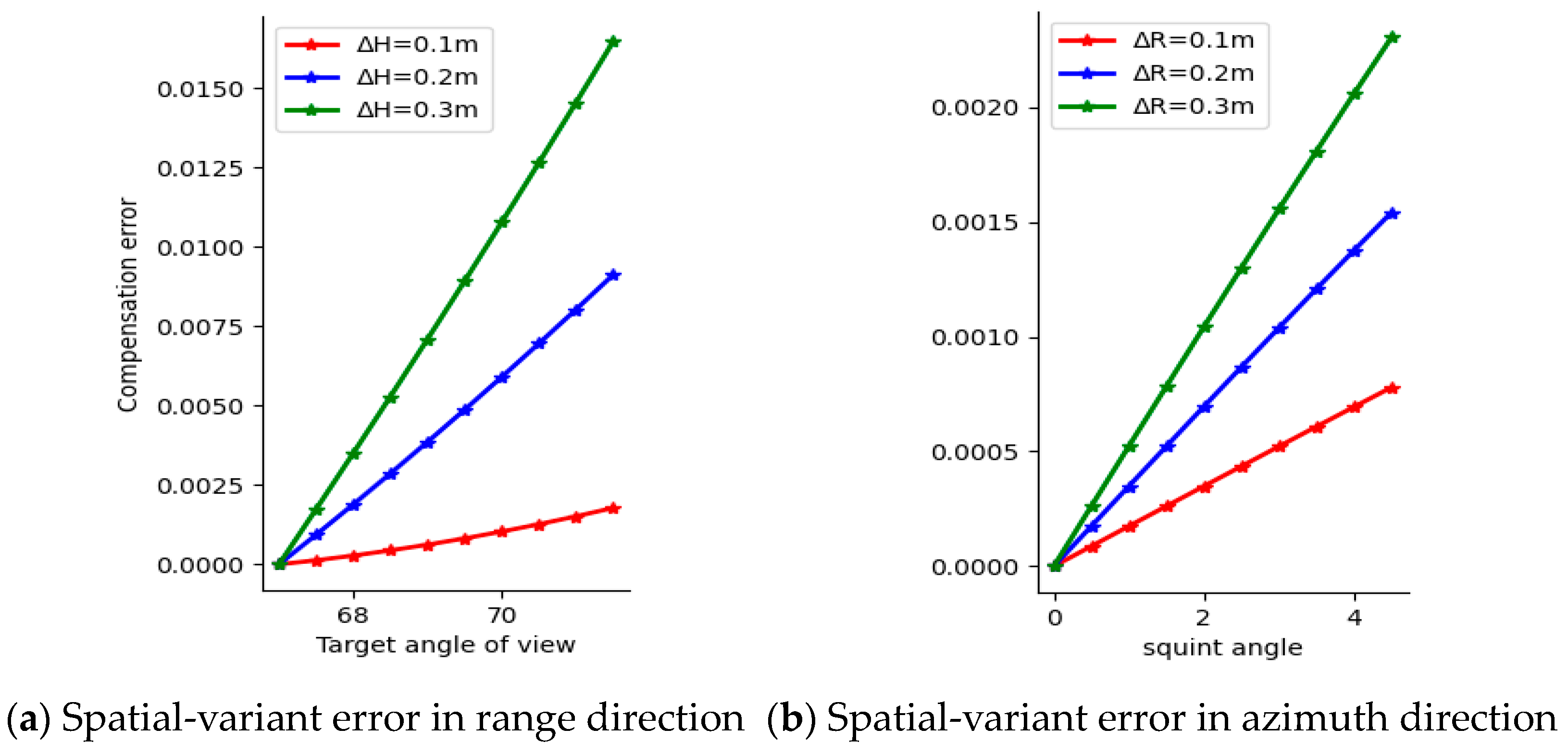
When imaging narrow scenes with traditional linear SAR, if the range beam is narrow (i.e., $\alpha \approx 0$), the spatial variability of slope errors for point targets at different range cells can be ignored, and a uniform phase-error estimation and compensation can be applied to points in the range direction. Similarly, if the azimuth beam is narrow (i.e., $\alpha \approx 0$), the spatial variability of motion errors for point targets in different azimuth cells can be ignored, and a uniform envelope and phase compensation can be applied to points within the azimuth beam. However, in order to expand the imaging range, the beam of CSAR is generally designed to be wide (around 10°), which makes the spatial variability of motion errors very significant. Assuming a radar beam of 10° with a center-looking angle of 67°, the errors in range and azimuth directions are shown in Figure 4.

From Figure 4, it can be observed that the slant-range error of the point target has a linear relationship with its position, and the farther the target is, the larger the slant-range error will be. At the same time, the slant-range error in the range direction has a more significant impact than that in the azimuth direction. When the height error is only 0.3 m, the slant-range error can reach 0.015 m, which is already larger than $\lambda /8$. This error can easily cause target defocusing. Therefore, in the process of circular SAR imaging, the spatial variance cannot be ignored.

3. CSAR Auto Focusing Method

The biggest drawback of the BP imaging algorithm is its slow computation time. If nonspace-variant errors are considered in every azimuth direction for each pixel, the optimization time will become unbearable. Therefore, preprocessing of SAR images is required to shorten the optimization time. In the case of large motion errors, the noise in SAR images is often more obvious, and the Prewitt operator is robust to noise and performs better than other operators in extracting feature points.

To improve the self-focusing effect of the CSAR image, it is necessary to compensate for not only the nonmotion error but also the motion error. However, if the spatially varying error is estimated for each range, the dimensionality of the space to be solved will be increased to $N\times M$ ($N$ is the number of azimuths and $M$ is the number of ranges) for radar data of size (N, M). This greatly increases the computational complexity and requires storing the back projection values of each pixel at each slow time.

In fact, the phase error is caused by the motion error of the carrier, which is essentially the slope distance error between the carriers. It is therefore possible to estimate the slant-range error of the UAV directly; this greatly reduces the difficulty of solving the problem. Assuming the value of the measured APC at slow moment k, the error value of the measured APC is $p_k={[x_k,y_k,z_k]}^T$ and the measured APC error is ${\overline{p}}_k=\sqrt{\mathbf{\Delta }{x}_k^2+\mathbf{\Delta }{y}_k^2+\mathbf{\Delta }{z}_k^2}$; then the compensated backward projection of the mth pixel at slow moment k is

$$b_{m,k}=s_k({\tau }_{m,k})e^{j\omega {\tau }_{m,k}}$$

(17)

where ${\tau }_{m,k}$ is the echo delay after correction for APC motion error. Calculated as shown is Equation (17).

$${\tau }_{m,k}=2\times \left|{\overline{p}}_k\right|/2$$

(18)

By accumulating the projection values of all slow moments to the m-th pixel through the BP algorithm, the total backward projection value of the mth pixel point can be obtained as

$$z_m={\displaystyle \sum _{k=1}^K{b}_{m,k}}$$

(19)

The sharpness value can be calculated from the image-pixel values and the sharpness value of the m-th pixel point is

$$f_m=z_m{z}_m^{*}$$

(20)

The sharpness is a good reflection of the focus effect of the SAR image, so that we transform the problem of calculating the carrier motion error into the problem of optimizing the image sharpness value. This paper uses particle swarm optimization (PSO) to optimize the model. PSO is a population-based, stochastic optimization method proposed by Kennedy and Eberhart. The great advantage of PSO over traditional optimization algorithms is that it can obtain the best acceptable solution on a global perspective, converge quickly compared to traditional iterative algorithms, have more accurate parameter estimates than traditional algorithms, and is more resistant to interference.

The concept of particle swarm optimization (PSO) originated from the foraging behavior of birds and fish. In PSO, each particle is a candidate solution in the search space, referred to as a particle, and their particles constantly move in the search space to find the optimal position. Each particle has a position $y_i=[y_{i1},y_{i2},\dots y_{iN}]$ and $v_i=[v_{i1},v_{i2},\dots v_{iN}]$, where $\mathrm{i}$ denotes the i-th particles and N denotes the number of unknowns. PSO starts by initializing a swarm of random particles, which are then updated iteratively to search for the optimal solution. During each iteration, every particle updates its position vector based on the two “best positions” available to it. The first is the position vector of the best solution found by that particle so far, known as pBest. The second is the position vector of the best solution found by the entire swarm up until that point, known as gBest. After the two best positions are found, the particles are updated from the n-th generation to the n + 1 st generation. The calculation methods for gBest and pBest are shown in Equations (21) and (22), respectively.

$$v_i^{n+1}=b{v}_i^n+c_1{r}_1(pBes{t}_i^n-y_i^n)+c_2{r}_2(gBes{t}^n-y_i^n)$$

(21)

$$y_i^{n+1}=y_i^n+v_i^{n+1}$$

(22)

In the equation, b represents the inertia weight factor, $c_1$ represents the acceleration weight factor for each particle, $c_2$ represents the acceleration weight factor for the whole swarm, and $r_1$ and $r_2$ represent two independent random numbers uniformly distributed within the range [0, 1]. To evaluate the quality of the particle swarm’s current position, the complex value of the sharpness $f=-f_m$ is used as the fitness value. A smaller value of the $-f_m$ represents that the current particle is closer to the optimal solution.

The specific steps of the PSO-based algorithm are shown below.

Step0: Initialize a set of particles, including position vector $y_i^0$ and velocity vector $v_i^0$.

Step1: Calculate the fitness value of each particle by Equations (21) and (22).

Step2: For each particle, its fitness value $f(y_i^n)$ is compared with the fitness value corresponding to its best position pBest, and if $f(y_i^n)$ is smaller, $y_i^n$ will be used as the current gBest.

Step3: For each particle, compare its fitness value $f(y_i^n)$ with the fitness value $f(pBes{t}_i)$ corresponding to the best position of the whole population, if $f(y_i^n)$ is smaller, $y_i^n$ will be used as the current gBest.

Step4: Update $y_i^n$,$v_i^0$ using Equations (15) and (16).

Step5: If $f(gBes{t}_i)$ meet the condition or the maximum number of loops is reached, the loop ends and returns gBest, otherwise go to Step1.

For linear SAR data, once the subaperture images are obtained through autofocusing, the final image result can be directly achieved by incoherent superposition. However, since CSAR data does not have traditional-defined azimuth and range directions, errors in the position of image pixels can be introduced due to the observation trajectory and sampling frequency, leading to image displacement and scaling of the subaperture images. The phenomenon is known as geometric distortion. For circular synthetic aperture radar (SAR) data, subaperture image registration is generally used to eliminate geometric distortion. Chen calculates the affine transformation coefficients between adjacent subapertures for image registration of the image. However, there are two problems with this method. First, because of the small number of feature points, a small number of feature points may lead to deformation of the alignment; Second, some subapertures may be completely out of focus, causing errors in the calculated affine transformation coefficients for adjacent subapertures and error may accumulate. To address this issue, this paper proposes a novel subaperture registration method suitable for CSAR.

Methods of SAR image matching can be divided into two categories: feature-based and area-based methods. Feature-based methods use similarities of features extracted from images to achieve CPs between images. Feature-based methods rely on the detection of highly repeatable and common features between images. However, after autofocusing of the subimages, there may be differences in intensity, resolution, rotation, and deformation, which makes it difficult to extract a large number of repeatable features. Area-based methods usually utilize similarity metrics to detect CPs between images through a template-matching strategy. When compared with feature-based methods, area-based methods have the following advantages: (1) area-based methods eliminate the need for extracting common features between images; (2) they can detect control points (CPs) within a small search region because adjacent subaperture images have position offsets of only a few or a few dozen pixels. Yuan proposes a robust SAR-matching method based on shape properties named DLSC which has been proven to have strong robustness within a small angle range. In this paper, DLSC is used to register subaperture images.

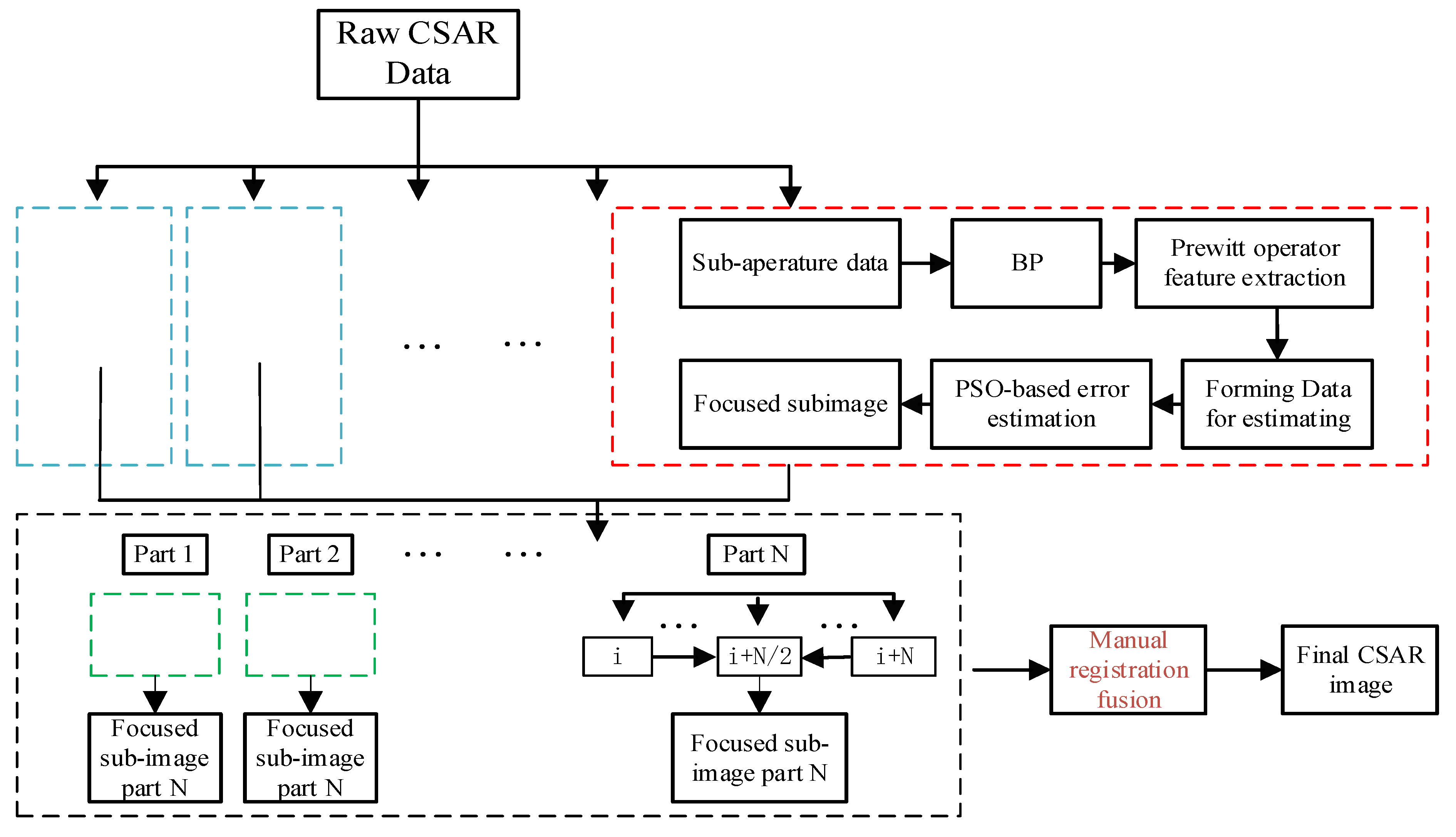
CSAR data is divided into M subapertures and partitioned into N parts. Each part consists of subapertures $[i,\cdots i+N/2,\dots i+N]$. Choose $i+N/2$ as a reference subaperture, registering all subaperture images in each part with respect to the reference subaperture by DLSC [17]. The accumulation results for each part are shown in Equation (17)

$$A={\displaystyle \sum _i^{i+N}(S_i/N)}$$

(23)

The final CSAR image is obtained by registering different parts and performing incoherent addition. The entire CSAR subaperture focusing and registration process is shown in the Figure 5 below.

4. Simulation Data Test

Firstly, simulation analysis was conducted on point targets with simulation parameters shown in

Table 1. Simulation Parameters Settings.

Parameter	Value	Parameter	Value
waveband	X	flight radius	600 m
bandwidth	0.75 GHz	flight height	300 m
PRF	333.3 Hz	velocity	7 m/s
slant-range	500~800 m

. Five point targets were set in the scene, with the reference point target (scene center) located at ${\mathrm{p}}_{\mathrm{c}}={[0,0,0]}^T\mathrm{m}$, and the positions of the other four nonreference point targets were ${\mathrm{p}}_1={[10,10,0]}^T\mathrm{m}$, ${\mathrm{p}}_2={[-10,10,0]}^T\mathrm{m}$, ${\mathrm{p}}_3={[-10,-10,0]}^T\mathrm{m}$, and ${\mathrm{p}}_4={[10,-10,0]}^T\mathrm{m}$. The imaging range of the BP algorithm was within the grid of $50\times 50$ m, and the resulting scene graph after imaging with the BP algorithm is shown in Figure 6a. All simulation and actual test algorithms in this paper are based on Matlab2021 and Windows 10 system.

As shown in Figure 6, the flight trajectory of CSAR was designed in a circular shape. To evaluate its performance, uniformly distributed random errors of [−0.1 m, 0.1 m] were introduced in the three directions of the APC flight trajectory. The imaging results of the point targets are shown in Figure 7a. The imaging graph of the point targets after adding errors is shown in Figure 7b.

The point targets set in the simulation had the same scattering characteristics in all directions. To reduce computational complexity, only the related pixels surrounding the five data points were used for phase estimation. A total of 50 pixels were chosen as new data for both ABP and the autofocusing method proposed in this article. The imaging results of the reference point target using these two methods are shown in Figure 8.

It can be observed that although the ABP method has a strong background noise suppression ability and produces images with a certain degree of focusing, it still exhibits significant variability errors in the range direction on each subaperture, leading to energy dispersion. In contrast, the proposed method in this article corrects spatial-variability errors effectively, resulting in good energy focusing and better imaging performance compared to the ABP algorithm.

For further quantification of algorithm performance, Figure 9 shows azimuth and range profiles of the central point target after using different algorithms, thereby further demonstrating the differences among the algorithms. Compared with ABP, the algorithm proposed in this chapter generates curves that are mostly symmetrical, with the narrowest main lobe width and obvious separation side lobe, and produces the best imaging results. It is evident that the algorithm proposed in this paper performs better compared to ABP.

Table 2. Quantification of algorithm performance.

Algorithm	Azimuth Resolution/cm	Range Resolution/cm	PSLR/dB
Proposed method	10.3279	11.3256	20.1548
ABP	14.5208	13.2154	13.4685

provides the imaging indicators for the strong scattering point. Comparing the data for two algorithms, it can be observed that the proposed algorithm in this paper has the least loss of PSLR and LSLR. The resolution results also indicate that the proposed algorithm’s results are the best.

5. Real Data Test

The X-band CSAR raw data were collected by an airborne CSAR data acquisition experiment which was mounted on an unmanned aerial vehicle(UAV) in the Chang’ an street district of Shijiazhuang. The CSAR system parameters are presented in

Table 3. CSAR Data Parameters Settings.

Parameter	Value	Parameter	Value
waveband	X	flight radius	600 m
bandwidth	0.75 GHz	flight height	300 m
PRF	333.3 Hz	velocity	7 m/s
slant-range	500~1000 m	TX frequency	9.6 GHz

, whereas the satellite image of the area under consideration is shown in Figure 10a. The region marked as Area 1 comprises a “T”-shaped cement ground that houses three vehicles, namely A, B, and C, along with four reflectors, A, B, C, and D. These reflectors are divided into groups and each group comprises a tetrahedral, a hexahedral, and a dihedral reflector. On the other hand, the second area consists of a house constructed from separate containers, as depicted in Figure 8c. Figure 8d shows the unmanned aerial vehicle (UAV) carrying the radar.

Due to limitation of the airborne CSAR system, the three-axis stabilizing platform remains inoperative. Consequently, the beam center direction of CSAR undergoes variations based on the attitude of the UAV, making it challenging to accurately point towards the observed scene’s center. Therefore, the motion error for CSAR imaging is considerable.

The number of APC selected for the imaging process was K = 10,000. The azimuth sampling frequency was set to be the same as that of APC, with subaperture synthesis being performed using 1000 azimuth directions as a unit. The two-dimensional space had a size of M = 801 × 801 pixels, with the imaging range being 50 × 50 m.

The subaperture BP-imaging result obtained after phase compensation using the platform’s initial GPS position and velocity is shown in Figure 9a. From the subaperture image, it is obvious that the accuracy of the CSAR without phase compensation is significantly inadequate. As a result, the resulting image is severely defocused, making it difficult to identify targets in the scene.

The parameters for the PSO algorithm are typically set based on experience ${\mathrm{c}}_1={\mathrm{c}}_2=2$, ${\mathrm{v}}_{\max }={\mathrm{my}}_{\max }$, $0.1\le \mathrm{m}\le 0.2$. To achieve a balance between avoiding getting trapped in local optima while also ensuring convergence speed, the inertial weight coefficient $\mathrm{b}$ can be set to linearly decrease with iteration count. The subaperture imaging after autofocusing is shown in Figure 11. The objective, designated within the red box, is three corner reflectors and a central building in the allocated area.

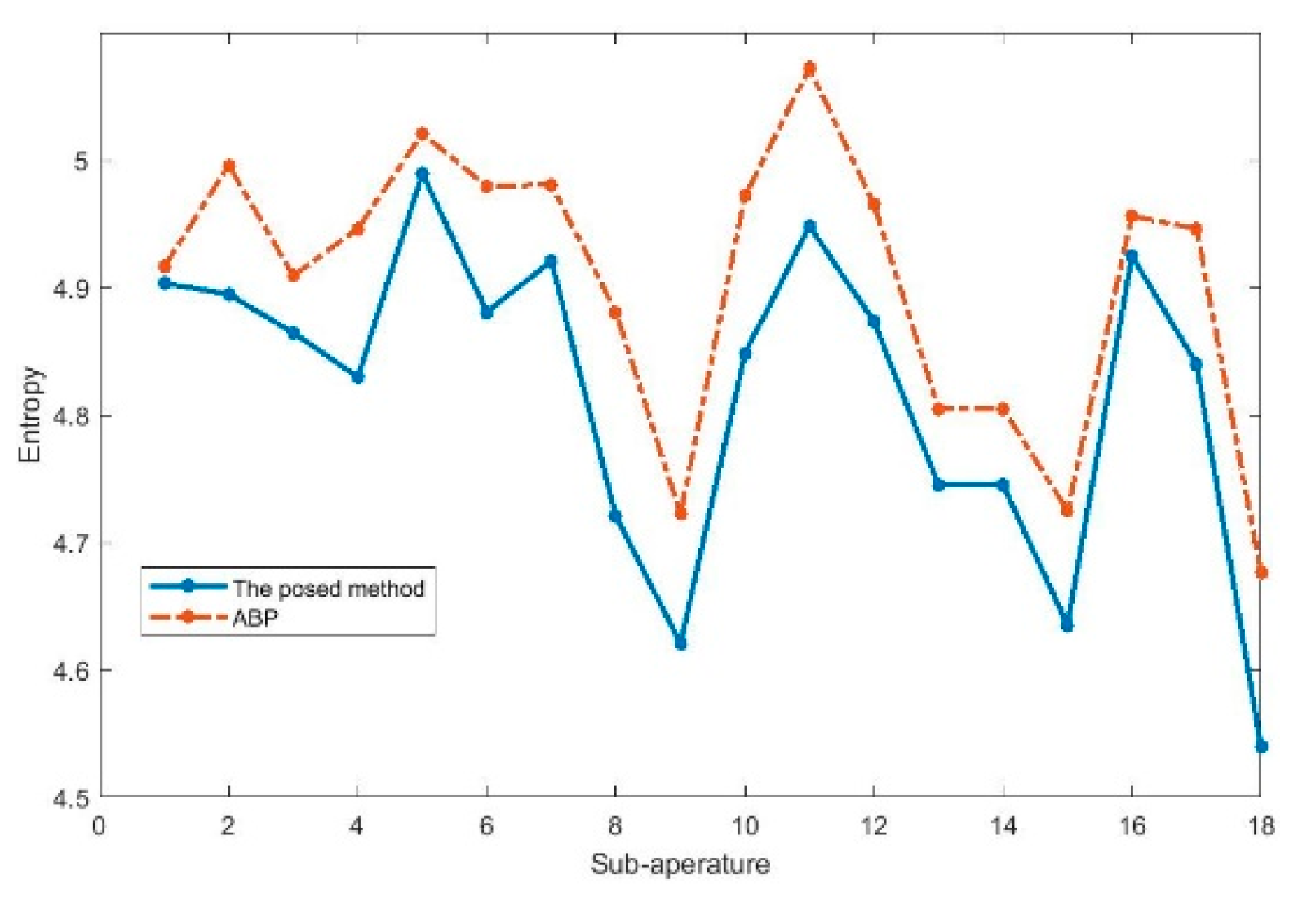
From Figure 11, compared to the ABP algorithm, the proposed method in this paper has a better focusing effect. Upon enlarging the building and corner reflectors, it becomes apparent that the proposed method in this paper has a superior focusing effect, as evidenced by the clear visibility of the corner reflectors and the well-defined building, which allows for more concentrated energy. To further demonstrate the effectiveness of the proposed method, separate entropy calculations were conducted for each subaperture, as illustrated in Figure 12. The results indicate that the proposed method outperforms ABP in terms of performance across all subapertures.

After obtaining the focusing results for each subaperture, registration was performed using both the method proposed in this paper and the method proposed by Chen. The results are illustrated in Figure 13, it can be observed from the figure that the proposed method not only effectively estimates and compensates for phase errors but also has superior image synthesis performance compared to other methods. From the three red boxes highlighted in the image, it can be seen that the urban buildings, corner reflectors, and vehicles have all been well-focused after being processed by the method in this article.

6. Conclusions

In this paper, we present a new autofocus and subaperture fusion method for CSAR data, based on the backpropagation algorithm. Firstly, this article analyzes the significance of spatial-variance error in the process of CSAR imaging. Firstly, this article analyzes the impact of spatial-variance error on the CSAR imaging process and concludes that this error cannot be ignored. Then, the Prewitt operator is used to extract features and the PSO algorithm is utilized to estimate the slant-range error, achieving subaperture autofocus. Finally, the BP-based CSAR imaging is completed through subaperture registration. In

Table 4. CSAR Data Parameters Settings.

Algorithm	Azimuth Resolution/cm	Range Resolution/cm	PSLR/dB
Proposed method	9.3279	12.2578	21.4697
ABP	14.5208	15.3474	13.2348

, the method in this paper obtains a large improvement in orientation resolution and distance resolution compared with other algorithms and also the PLSR of the processed images in this paper is improved.