1. Introduction
A Synthetic Aperture Radar (SAR) can perform high-resolution imaging of long-range scenes throughout the day, in all weather. With the continuous growth of application requirements, people’s demand for SAR high-resolution imaging is increasingly urgent [
1,
2,
3,
4]. However, the high resolution poses a great challenge to the instantaneous bandwidth and sampling rate of the radar system. SFCWSAR (Stepped Frequency Continuous Wave Synthetic Aperture Radar) can provide high-resolution imaging without increasing the radar’s instantaneous bandwidth and sampling rate. The governing principle is to transmit multiple sub-bandwidth signals and synthesize the echo signals into a large-bandwidth signal through signal processing technology [
5,
6,
7,
8].
However, even if the SFCWSAR system is adopted, the amount of data that the system needs to process is not reduced in order to obtain the same resolution. This poses a great challenge to the memory and operation efficiency of the system, especially in the case of high-resolution imaging of wide-format scenes [
9,
10].
Compressed sensing theory shows that when the imaging scene meets the sparsity condition, the SAR image can be reconstructed with high precision with a small amount of radar echo data. Applying compressed sensing theory to SAR (Compressed Sensing Synthetic Aperture Radar, CS-SAR) can effectively reduce the amount of data to be processed and the pressure on the computer memory [
11,
12,
13,
14].
When SFCWSAR transmits one sub-pulse, the slant range between the radar and the target changes, and the change in the slant range during the sub-pulse transmission will inevitably affect the quality of the synthesized bandwidth. However, for the SFCWSAR radar system, the existing sparse reconstruction model cannot compensate the phase error of each sub-pulse in the same pulse group of SFCWSAR due to the relative motion between the radar and the target, which seriously reduces the imaging quality. Furthermore, the precise observation matrix adopted by the existing sparse reconstruction model occupies too much computer memory, and the algorithm operation efficiency needs to be improved [
15,
16].
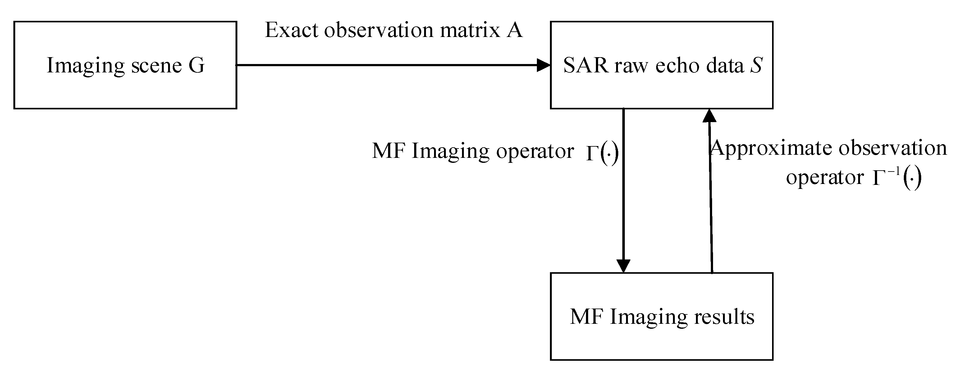
The team of the academician Wu Yirong from the Institute of Electronics, Chinese Academy of Sciences has proposed a sparse imaging method based on approximate observation operators through the research on traditional matched filter imaging algorithms. This method greatly reduces the dimension of the measurement matrix, reduces the computational load and memory footprint of the CS-SAR algorithm, and improves the computational efficiency of the algorithm; it has thus received extensive attention [
17,
18,
19]. In addition, the approximate observation operator is derived from the traditional matched filter imaging algorithm. In this paper, it is applied to the sparse reconstruction of SFCWSAR, which makes it possible to compensate for the phase error of each sub-pulse in the same pulse group due to the relative motion of the radar and the target [
20,
21].
The above problem can be solved using an approximate observation operator instead of the existing precise observation matrix, and the construction of an approximate observation operator needs to obtain the accurate Doppler center frequency. However, the Doppler center frequency has errors because the carrier aircraft is easily affected by airflow and its mechanical vibration in the air. If the Doppler center frequency value obtained by theoretical calculation is directly used to construct the approximate observation operator, the theoretical model of imaging will not match the actual imaging process, which will seriously affect the sparse reconstruction [
22,
23]. Therefore, the Doppler center frequency needs to be estimated and compensated. The SAR carrier is generally equipped with a navigation and measurement system to detect the fast and slow variation of the antenna phase center and the in-plane and non-planar components of the disturbance and to compensate accordingly. However,
(1) Equipping with high-precision inertial navigation equipment increases the cost of the system hardware.
(2) Some flight platforms are unable to carry inertial navigation equipment with a large weight and volume due to load limitations, such as the SRUAV (Small Rotor Unmanned Aerial Vehicle).
Therefore, it is necessary to study data-driven Doppler centroid frequency estimation methods in consideration of the cost and load capacity of some SAR systems.
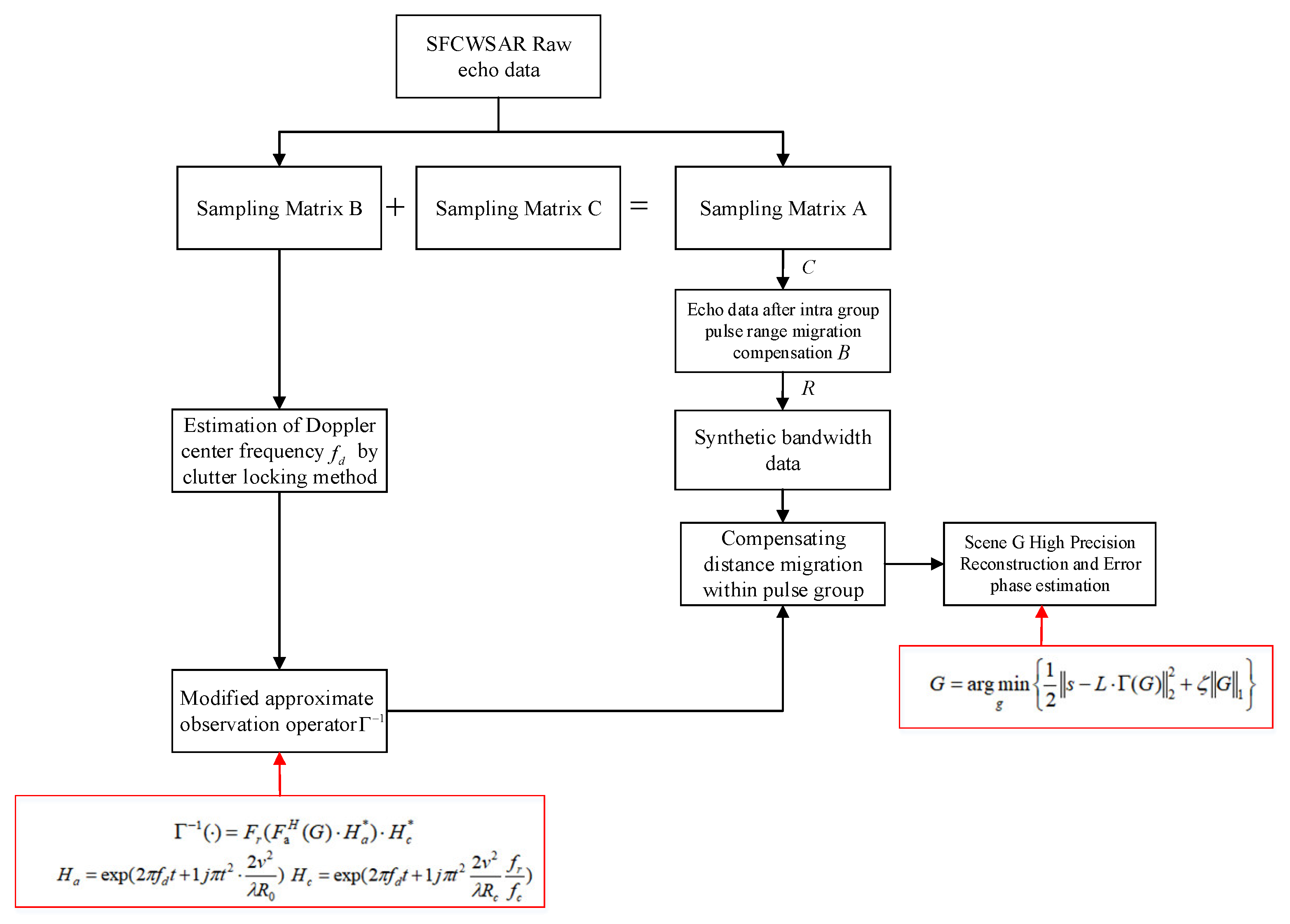
In view of the above problems, a sparse reconstruction algorithm based on the approximate observation operator SFCWSAR is proposed in this study. The algorithm compensates for the range migration within the pulse group and corrects the Doppler center frequency. In this method, the approximate observation operator is used to replace the precise observation operator, which not only improves the efficiency of scene reconstruction but also reduces the memory usage of the system. Then, the range migration within the SFCWSAR group is compensated, and the compensated echo data are used for the SFCWSAR sparse reconstruction. Furthermore, the narrowband sub-pulse signal under the full sampling condition is obtained through the construction of the sampling matrix, while the undersampled echo data is obtained. The Doppler center frequency is estimated using the complete narrowband echo signal. The approximate observation operator is modified using the estimated Doppler center frequency, and then the corrected approximate observation operator is used for the sparse reconstruction of the scene. The measured data show that the proposed algorithm can effectively reconstruct the scene with high precision and greatly improve the computational efficiency.
2. SFCWSAR Signal Model and Range Migration Correction in the Pulse Group
2.1. Stepped Frequency Continuous Wave SAR Signal Model
This section briefly introduces the signal model of SFCWSAR:
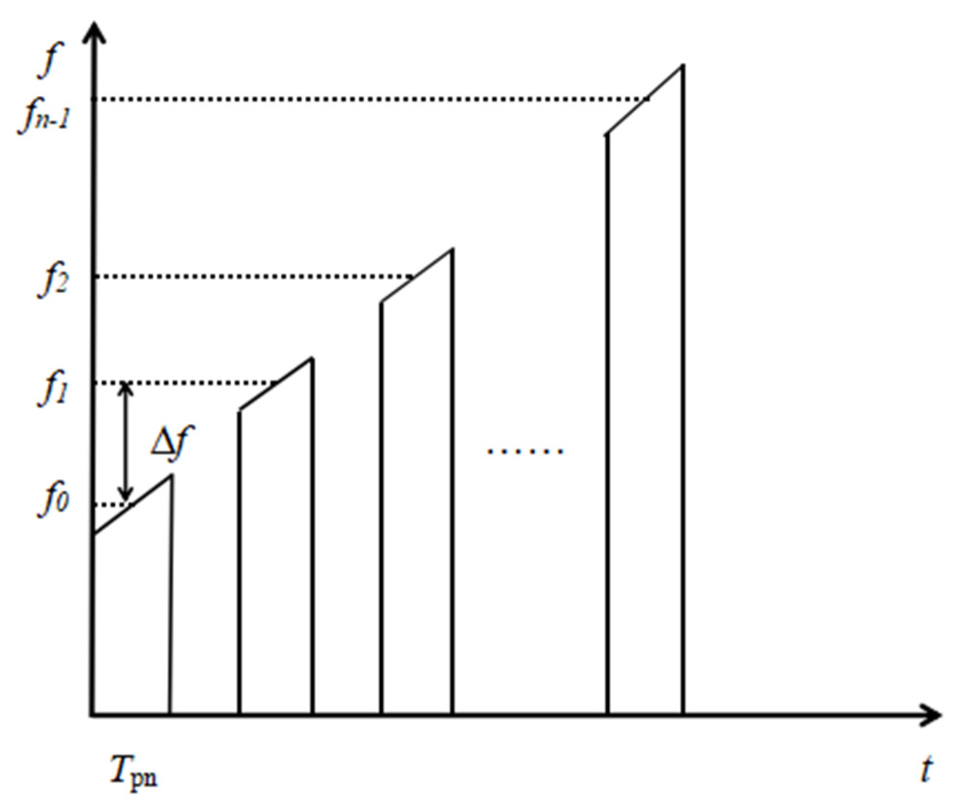
It is assumed that the sub-band pulse chirp bandwidth is B, the pulse length is Tpn, and the center frequency of each sub-pulse changes in steps of Δf. The center frequency of the broadband chirp signal obtained after narrowband sub-pulse synthesis is fc, the bandwidth is Bn, and the pulse length is Tp.
The center frequency of the kth signal in the n narrowband pulse signals is:
It is assumed that the radar transmits the Kth signal of n narrowband pulse signals at time tmk = tm + (k − 1)Tpn, 1 ≤ k ≤ n), the frequency modulation is , and the range fast time is .
The transmitted signal is:
Figure 1 shows the pulse waveform of the FM step frequency signal.
The target echo signal with distance
R is:
The reference function is:
Then, the received baseband signal is:
2.2. Range Migration Correction in the Pulse Group
Section 2.1 briefly introduces the SFCWSAR signal. Different from other systems, SFCWSAR transmits multiple sub-bandwidth signals, and the echo signal is synthesized into a large-bandwidth signal through signal processing technology. During the transmission of each sub-pulse, the slant range between the radar and the target changes, and the change in the slant range during the transmission of the sub-pulse will inevitably affect the quality of the synthesized bandwidth.
It is assumed that the echo time delay of the target at distance
R is
, there is relative motion between the radar and the target, and the relative radial velocity between the two is
v. If the above signal is not transmitted when the distance from the target is
R and is delayed by
Tr when the target distance is
R, then the echo delay at this time is no longer
but:
indicates the time delay caused by the relative motion between the radar and target.
Therefore, the echo at this time is no longer Equation (5) but becomes
It can be seen from Equations (7) and (8) that there is an additional in the time domain and a constant phase term in the phase . The phase discontinuity and the time delay are caused by the relative motion between the radar and the target. These phases easily cause the target range to decrease in amplitude, the main lobe to widen, and even the divergence and distortion of the waveform. In order to improve the imaging quality of SFCWSAR, the phase error must be compensated.
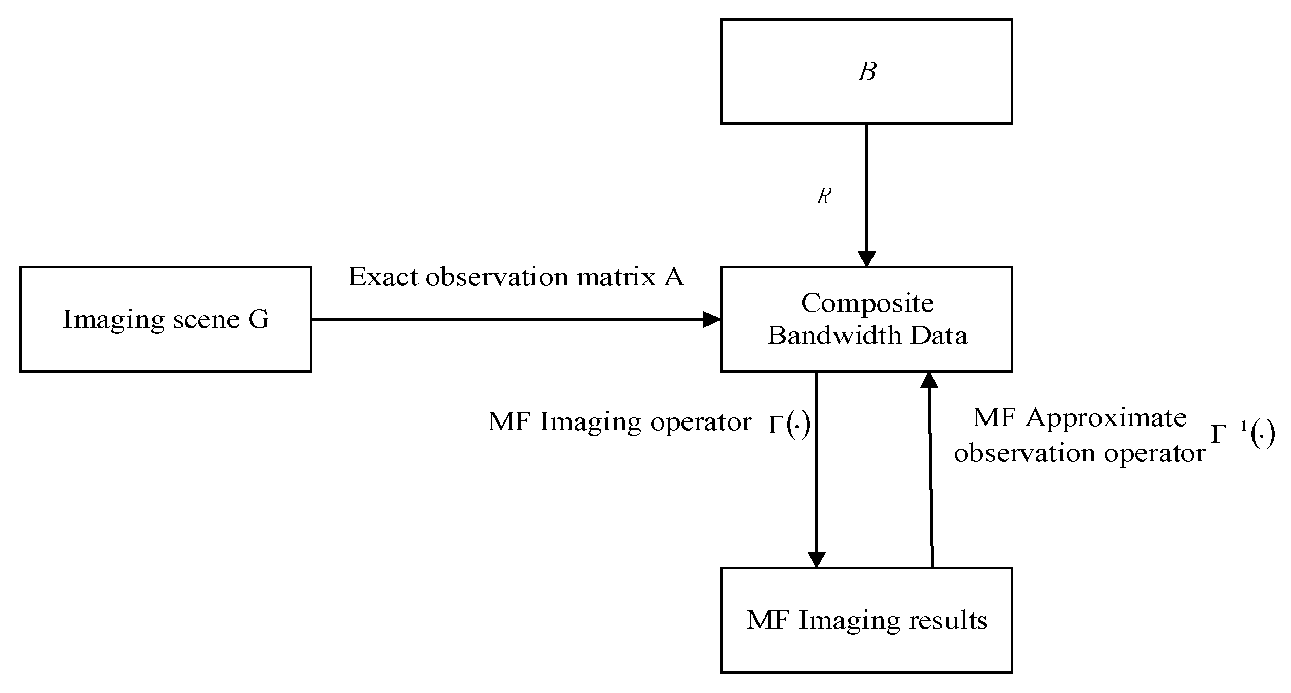
For SFCWSAR, traditional sparse reconstruction algorithms based on precise observation operators cannot compensate for the above errors, resulting in a sharp decline in the quality of sparse reconstruction. In order to realize the compensation of the above phase error, the approximate observation operator is used in this paper instead of the precise observation matrix to realize the sparse reconstruction of SFCWSAR. It is possible to compensate for the range migration within the SFCWSAR pulse group because the approximate observation operator is derived from the imaging algorithm.
5. Doppler Center Frequency and Approximate Observation Operator
Section 3 discusses the sparse reconstruction algorithm of SFCWSAR based on approximate observation operator. The Doppler center frequency
fd is an important parameter for establishing the approximate observation operator.
5.1. Doppler Center Frequency
The synthetic aperture radar uses the principle of synthetic aperture to improve the azimuth resolution of the radar. Pulse compression techniques are used to improve the range resolution. During azimuth compression, the Doppler center frequency of the target echo must be accurately known to achieve matched filtering. The error of the Doppler center frequency will reduce the signal-to-noise ratio of the image, increase the azimuth ambiguity, and make the target position on the image shift, which will seriously reduce the imaging quality. For the SFCW sparse reconstruction model with an approximate observation operator, the Doppler center frequency, as an important parameter, deeply affects the accuracy of the approximate observation operator construction. The misalignment of the Doppler center frequency will lead to the mismatch between the theoretical model and the mathematical model, which will seriously affect the effect of sparse reconstruction.
However, the existing approximate observation sparse reconstruction models do not consider the difference between the Doppler center frequency value and the theoretical value caused by the non-ideal motion of the carrier aircraft. Furthermore, the phase error introduced by the non-ideal motion of the SAR carrier platform will lead to an estimation error. The Doppler center frequency can be calculated by measuring the relative position and velocity matrix centered between the target and the antenna, or it can be directly extracted from the SAR raw data. The SAR carrier is generally equipped with a navigation and measurement system to detect the fast and slow variation of the antenna phase center and the in-plane and non-planar components of the disturbance and to compensate accordingly. However, high-precision inertial navigation equipment will increase the hardware cost of the system, and some micro SAR systems cannot carry inertial navigation equipment with a large volume and weight. The data-driven autofocus algorithm estimates the phase error from the echo data. Although it increases the complexity of the algorithm, it can meet the requirements of high-resolution imaging without increasing the cost of system hardware [
27].
Based on the above problems, this paper proposes an SFCWSAR sparse reconstruction method using sub-band data to estimate Doppler parameters and modify the approximate observation operator. First, the method sets the sampling matrix so that the sub-band echo data under the full sampling condition can be obtained simultaneously when the undersampled SFCWSAR echo data are obtained. Then, the Doppler parameters caused by the carrier’s non-ideal motion are corrected by using the sub-band echo data under the full sampling condition. The approximate observation operator is constructed by using the modified Doppler center frequency. Finally, SFCWSAR sparse reconstruction is realized by using the modified approximate observation operator.
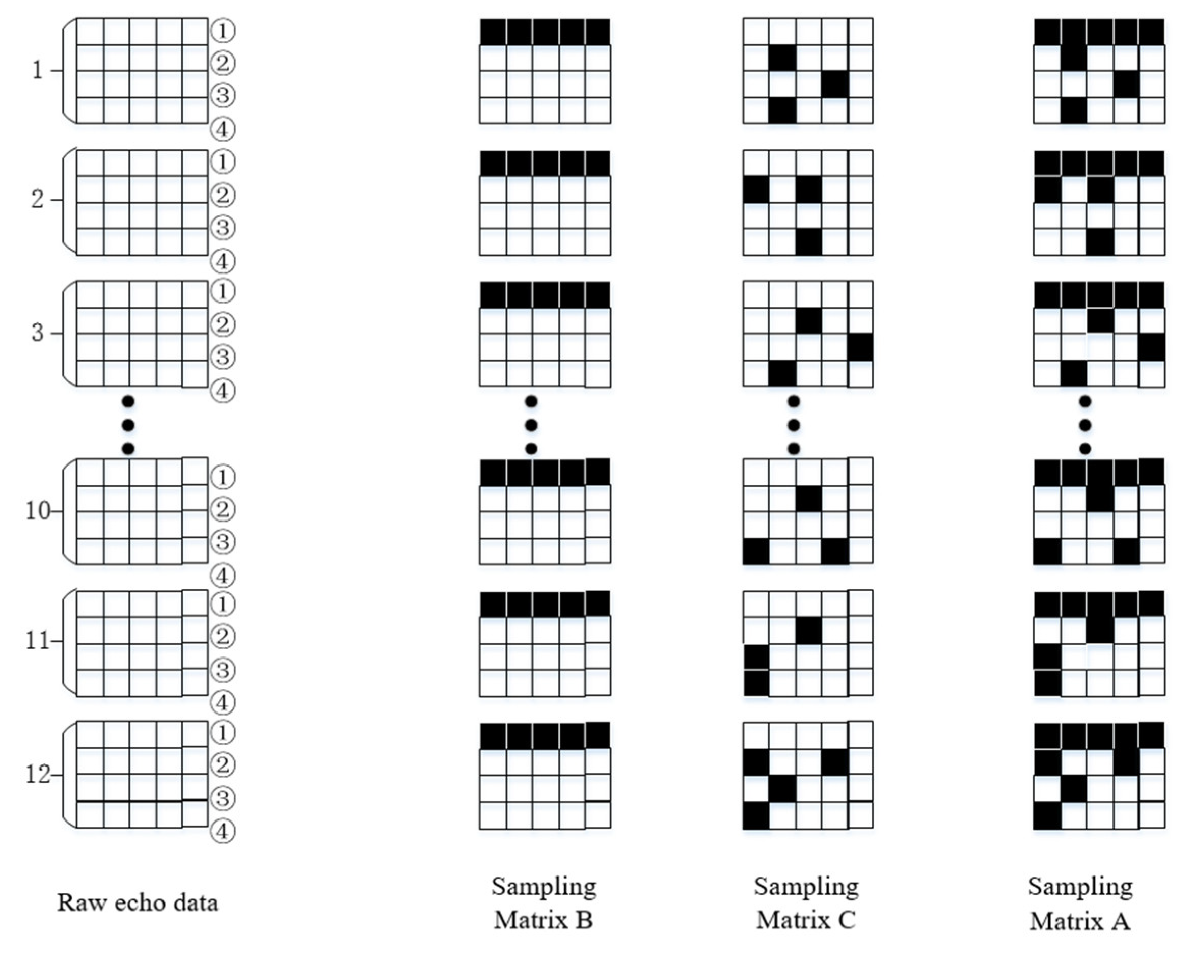
5.2. Setting of the Algorithm Sampling Matrix
In order to obtain the complete sub-pulse data while obtaining the sparse sampling data, the sparse sampling matrix in this paper is set to three types: A, B, and C. The three are satisfied, where B is the sampling matrix for obtaining the complete sub-pulse echo data and C is the matrix for the sparse sampling of the data from the whole echo, except for the complete sub-pulse echo. A can be obtained by computing C and B. The schematic diagrams of the three matrices, A, B, and C, are shown in
Figure 4.
Using the sampling matrix shown in
Figure 4, to facilitate the description of SFCWSAR data, the number of azimuth pulse groups is set to 12, the number of subpulses per pulse is set to 4, and the number of range sampling points is set to 5.
We can obtain the sub-band echo data under full sampling conditions while obtaining the sparse sampling matrix. Therefore, the narrowband echo data under full sampling can be used to estimate the Doppler center frequency.
5.3. Doppler Center Frequency Estimation
Because it is often difficult for the speed and detection accuracy of the equipment to meet the requirements of high-resolution imaging, in order to obtain an accurate Doppler center frequency, this algorithm chooses to use sub-band echo data to estimate the Doppler center.
Doppler center frequency estimation methods mainly include the frequency domain estimation method and time domain estimation method.
Due to the small size of the UAV platform, it is easily affected by airflow disturbance and its mechanical vibration. Therefore, there are approximately periodic changes in the Doppler center of the azimuth signal, so the phase-based time domain correlation method cannot accurately estimate the Doppler center frequency. In addition, the influence of the beam-pointing jitter on the amplitude of the azimuth signal is much smaller than the influence on the signal phase. Therefore, the amplitude-based clutter locking method is applied to estimate the Doppler center in this paper [
27].
The specific method is: first, obtain the azimuth Doppler spectrum of the echo of the sub-band signal under the full sampling condition, and the center frequency of the azimuth signal is approximately equal to its spectrum center of gravity [
28]. Therefore, the center frequency can be estimated by taking the azimuth signal of a range gate to calculate its spectrum center of gravity. However, in fact, the front end and back end of the acquired azimuth signal inevitably contain some incomplete Doppler histories. These incomplete Doppler histories constitute an important source of estimation bias. In order to improve the estimation accuracy, the average power spectrum of all or part of the azimuth signals of the range gate can be used. Finally, the energy center of the above power spectrum can be found. By retrieving the points with equal spectral energy integrals on both sides, the frequency corresponding to this center is the Doppler center frequency estimated by the clutter locking method.
Using the above method, the Doppler center frequency is estimated as using the narrow band sub-pulse, and is substituted into the approximate observation operator. The modified approximate observation operator is recorded as . will be used for the sparse reconstruction of the scene.
5.4. Algorithm Pseudocode and Flow Chart
Section 5.4 further explains the algorithm in this paper by using the algorithm pseudo code and flow chart.
The pseudo code of the algorithm 2 proposed in this paper is shown in the following Algorithm 2:
| Algorithm 2 Sparse reconstruction algorithm based on range migration compensation and Doppler center frequency correction in the pulse group |
Step 1:
1: For SFCWSAR echo data, use sampling matrix A to conduct sparse sampling for the echo. The narrowband echo data EB and the undersampled SFCWSAR echo data EA are obtained under the condition of full sampling.
2: The EB is used to estimate the Doppler center frequency , and the estimated is used to modify the approximate observation operator to obtain the modified approximate observation operator .
3: The echo data E is obtained by range migration compensation and bandwidth synthesis within the pulse group for EA.
Step 2: Initialization: i = 0, V0 = 0, t0 = 1,
Reconstruction of scene scattering coefficient based on FIST
4:
5:
6:
7: i = i + 1,
8: if , the solution is completed,
9: else returns 4. |
The algorithm flow chart is shown in
Figure 5.
6. Measured Data Verification
In this section, the simulation and measured data are used to verify the effectiveness of the proposed algorithm.
Section 6.1 presents the simulation data verification. The approximate observation operator is used instead of the exact operator to realize the correction of the range migration within the SFCWSAR pulse group and to realize the sparse reconstruction of the scene under the condition of an undersampling rate.
Section 6.2 shows the verification of the measured data, and the measured data of the side-view airborne SFCWSAR is selected to verify the proposed algorithm. Using the sub-band echo data under the full sampling condition mainly realizes the correction of the Doppler center and improves the sparse reconstruction effect. Furthermore, the flight speed of the carrier aircraft in the measured data is low, and the range migration within the pulse group can be ignored by calculation, which will not affect the imaging results. Therefore, only the Doppler operator correction approximate observation operator part of the proposed algorithm is verified in
Section 6.2.
6.1. Simulation Data Verification
The parameters of the simulation experiment system are shown in
Table 1.
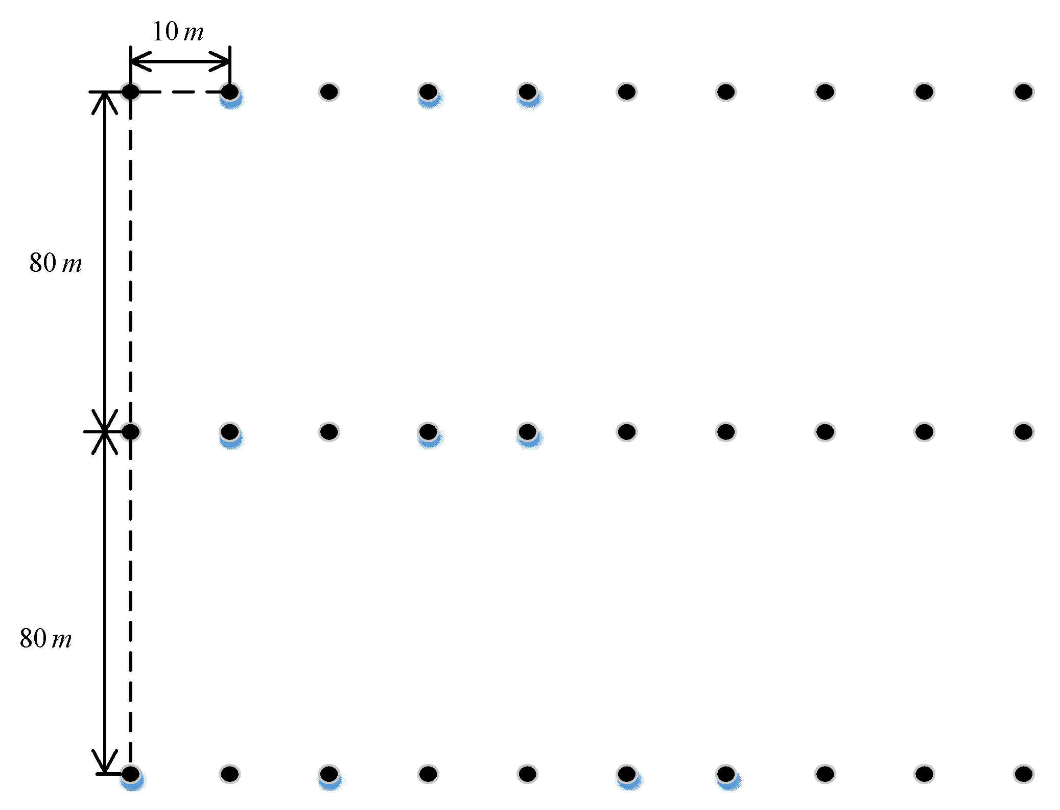
A total of 30 point targets are designed in the experimental scene, and their geometric distribution is shown in
Figure 6.
During the experiment, the measured data are extracted in the azimuth direction, and the echo data extraction rate is
.
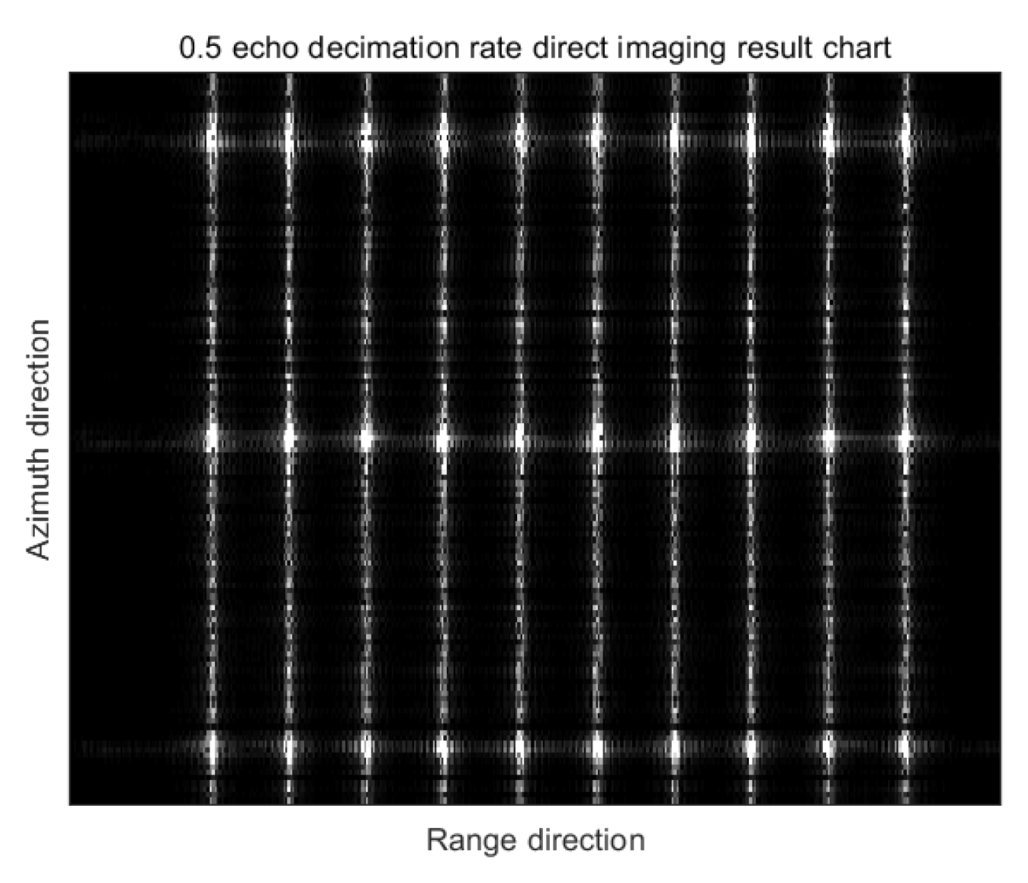
represents the fully sampled echo data. The decimation rate is chosen to be 0.5. When the echo decimation rate is equal to 0.5, the result of the imaging processing directly on the echo data under the undersampling condition is shown in
Figure 7.
Figure 7 shows that when the echo decimation rate is 0.5, the echo data under the undersampling condition is directly imaged, and the image quality is degraded due to the noise caused by the undersampling. Furthermore, the phase discontinuity caused by the relative motion of the radar and the target within the pulse group broadens the main lobe and even causes the divergence distortion of the waveform, which further reduces the image quality.
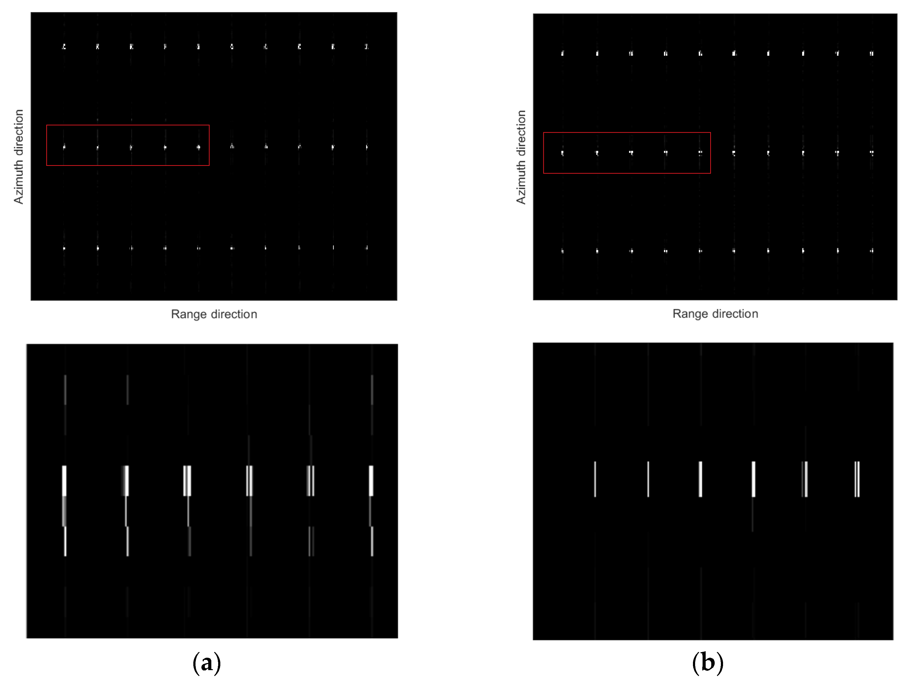
The algorithm proposed in this paper uses the approximate observation operator to replace the precise observation operator in the traditional CSSAR to sparsely reconstruct the scene from the data under the above-mentioned undersampling condition. The algorithm that directly uses the approximate observation operator to realize the sparse reconstruction of the scene is called Algorithm 1. The algorithm proposed in this paper that first corrects the range migration within the SFCWSAR pulse group and then uses the approximate observation operator to perform sparse imaging processing is called Algorithm 2. The sparse reconstruction results of each algorithm and the enlarged area in the red box in the results are shown in
Figure 8.
As shown in
Figure 8, the approximate observation operator is selected for CSSAR sparse reconstruction, which can realize scene reconstruction with a low data volume. For CSSFCWSAR, using the approximate observation operator can greatly reduce the memory usage of the computer when the algorithm is running and greatly improve the running efficiency of the algorithm. In addition, for the special signal form of SFCWSAR, different pulses in the same pulse group appear discontinuous in the phase due to the relative motion between the radar and the target. The phase error can be compensated by adopting the approximate observation operator.
Figure 8 shows the sparse reconstruction map of the scene and an enlarged view of the red boxed area in the target scene, and Algorithm 2 shows a better sparse reconstruction effect. Since Algorithm 1 does not compensate for the phase error between different pulses in the same pulse group, the target range decreases in amplitude, the main lobe broadens, and the waveform diverges and distorts, resulting in a corresponding decrease in the reconstruction effect of the point target. Algorithm 2 uses the approximate observation operator to compensate for the phase errors of different pulses in the same pulse group and then further realizes the sparse reconstruction of the target. Since the error phase is compensated, the sparse reconstruction result of Algorithm 2 is significantly improved compared with Algorithm 1. The algorithm in this paper achieves high-precision sparse reconstruction of the target scene, reduces the computer memory footprint, and improves the efficiency of the algorithm simultaneously.
6.2. Measured Data Verification
In this section, the effectiveness of the proposed algorithm is verified by the airborne SFCWSAR measured data. The system parameters are shown in
Table 2.
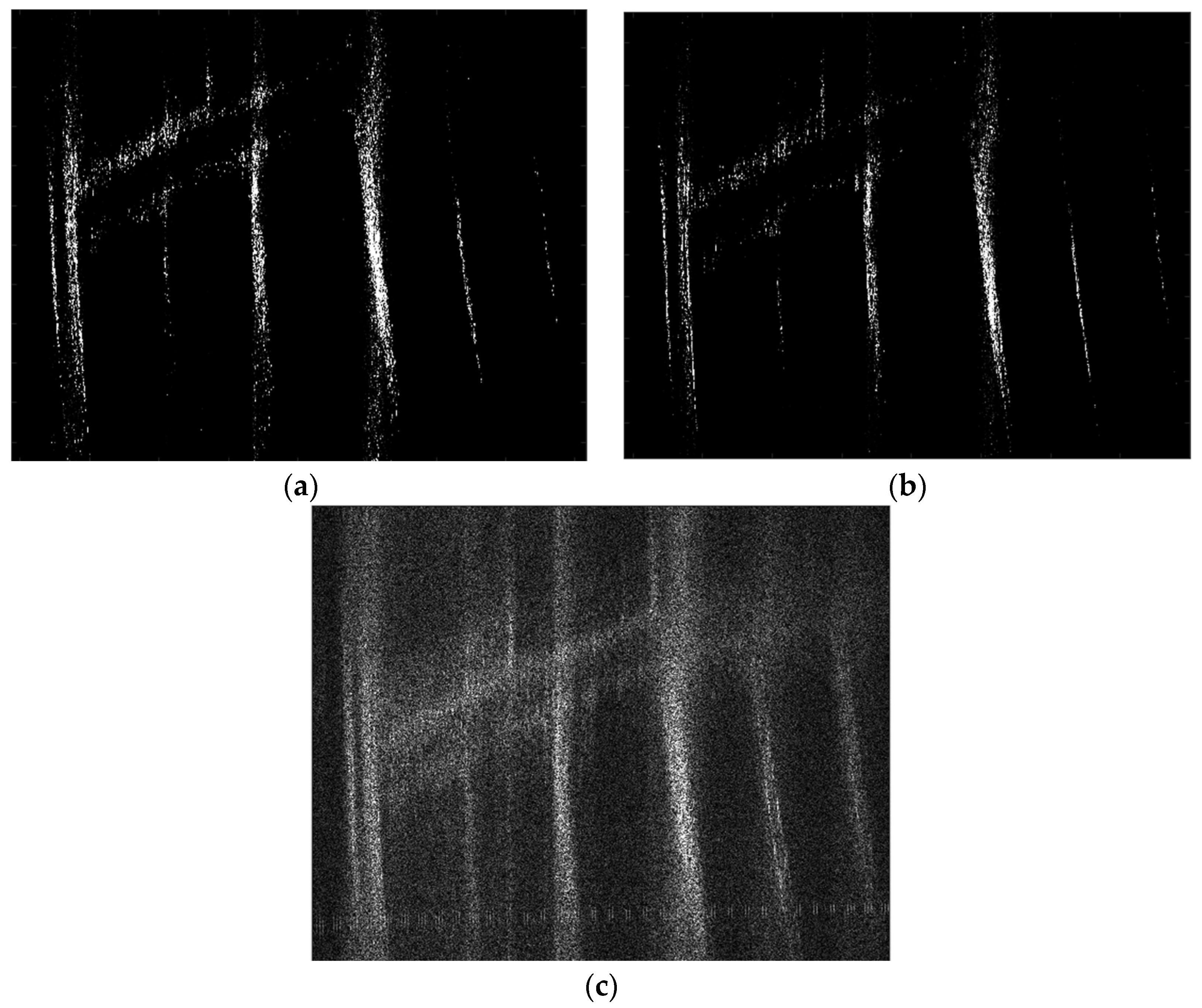
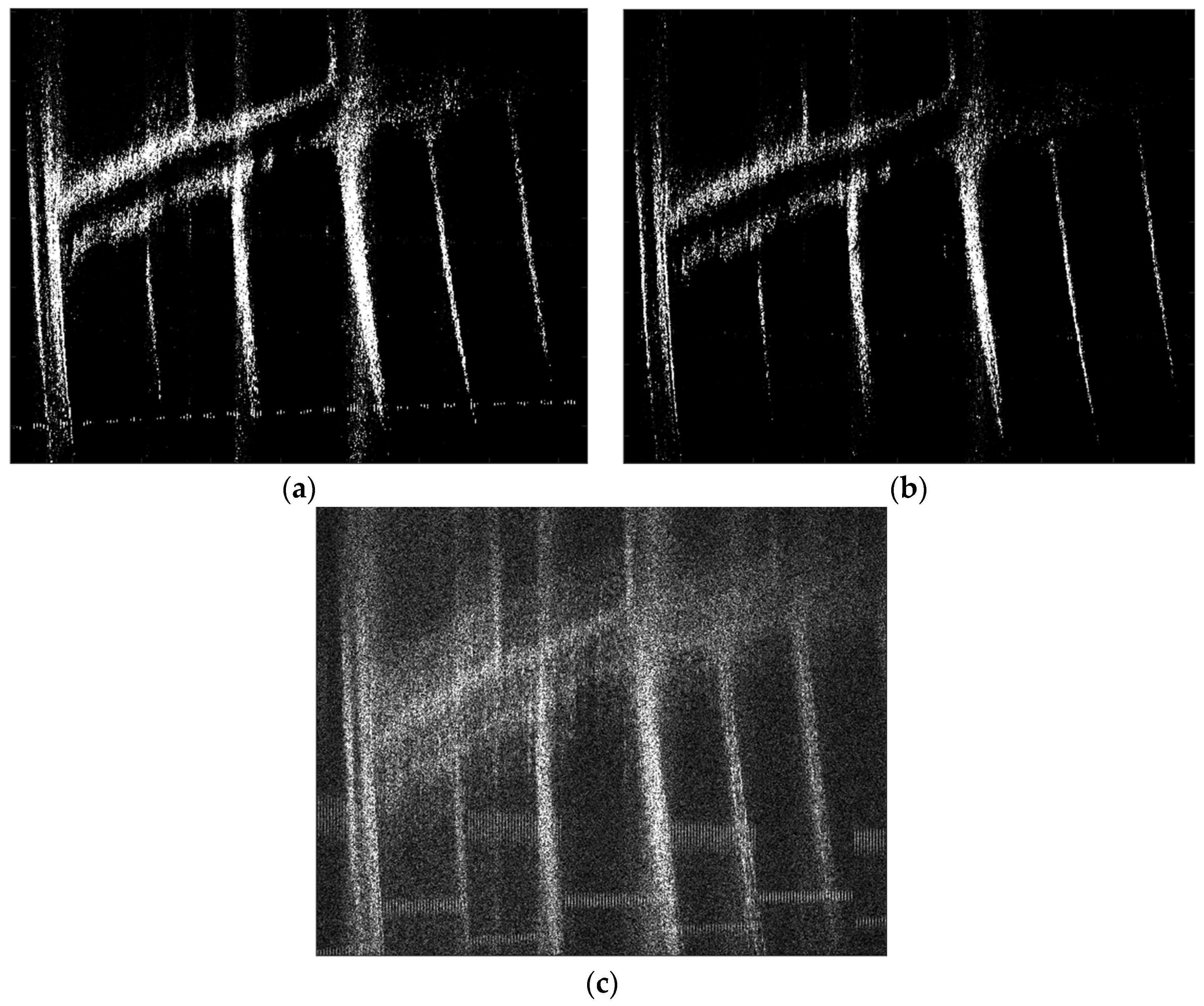
The exact observation operator in the traditional sparse compressed sensing model is replaced by the exact observation operator. The extraction rates are selected as 0.3, 0.5, and 0.7, respectively. In order to compare the convergence speed and accuracy of each algorithm, the number of iterations is unified to 10 times. The sparsity is set to 1572 (this parameter determines the FIST threshold). The algorithm that does not correct the Doppler center frequency in the SFCWSAR approximate observation operator is called Algorithm 1, and the algorithm in this paper is called Algorithm 2. Algorithm 1 and Algorithm 2 are used to image the SFCWSAR data, respectively. Due to the influence of the motion error, the image is defocused. In order to compare the sparse reconstruction performance of each algorithm, the sparsely sampled SFCWSAR data, after sparse reconstruction, adopted the sparse autofocus algorithm [
16] to perform motion compensation on the SAR data. Algorithm 2 selects the twelfth sub-pulse in each pulse group as the fully sampled narrow band pulse signal, and the sub-pulse signal accounts for 4.1% of the original echo data. It should be noted that although the algorithm obtains the narrow band pulse signal under the full sampling condition, the undersampling rate of the overall signal is consistent with the comparison algorithm.
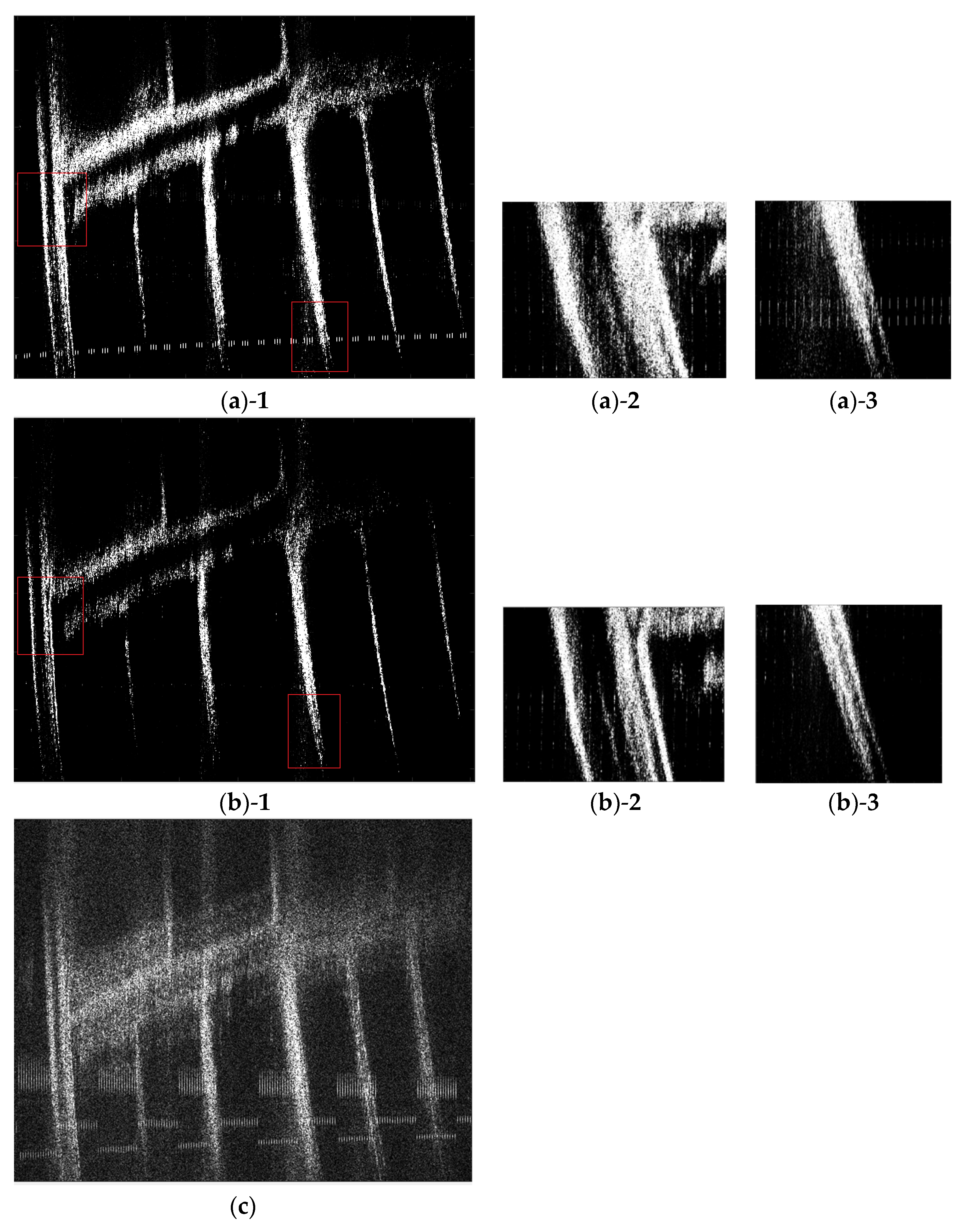
The sparse reconstruction maps of each algorithm are shown in
Figure 9,
Figure 10 and
Figure 11. The imaging scene is a field in China.
Figure 11 shows the sparse reconstruction map and the enlarged area map in the red box.
Figure 9c,
Figure 10c and
Figure 11c show that the data under the undersampling condition are directly imaged, and the noise caused by the undersampling leads to a significant decrease in the quality of the imaging results. By observing (a) and (b) of
Figure 9,
Figure 10 and
Figure 11, it can be seen that using the approximate observation operator instead of the precise observation operator can use the data under the undersampling condition to reconstruct the scene with high precision. Using approximate observation operators can greatly reduce the amount of computer memory occupied by the algorithm when it is running and improve the running efficiency of the algorithm.
By comparing and observing (a) and (b) in
Figure 9,
Figure 10 and
Figure 11, Algorithm 2 has a better sparse reconstruction effect than Algorithm 1. The reason for the result is that the approximate observation operator is derived from the imaging algorithm, and the Doppler center, as the core parameter of the imaging algorithm, is naturally an important parameter for the establishment of the approximate observation operator. However, the non-ideal movement of the carrier aircraft in the air, including the position deviation of the carrier aircraft from the ideal track, the change in the center of the radar beam, or the errors caused by the mechanical vibration of the carrier aircraft itself, can cause the Doppler center frequency to shift. Algorithm 1 selects the Doppler center frequency obtained by the theoretical calculation to construct the approximate observation operator. The mismatch of the Doppler center frequency will reduce the signal-to-noise ratio of the image, increase the azimuth ambiguity, and make the target on the image. The position is offset. The above reasons cause the error between the approximate observation operator and the theoretical imaging model. Therefore, the sparse reconstruction quality of Algorithm 1 needs to be improved. Algorithm 2 uses the sub-band data under full sampling conditions to estimate the Doppler center frequency using the clutter locking method. Furthermore, the estimated Doppler center frequency is used to approximate the construction of the observation operator, which improves the reconstruction algorithm and the mathematical model. Therefore, it has a better sparse reconstruction effect.
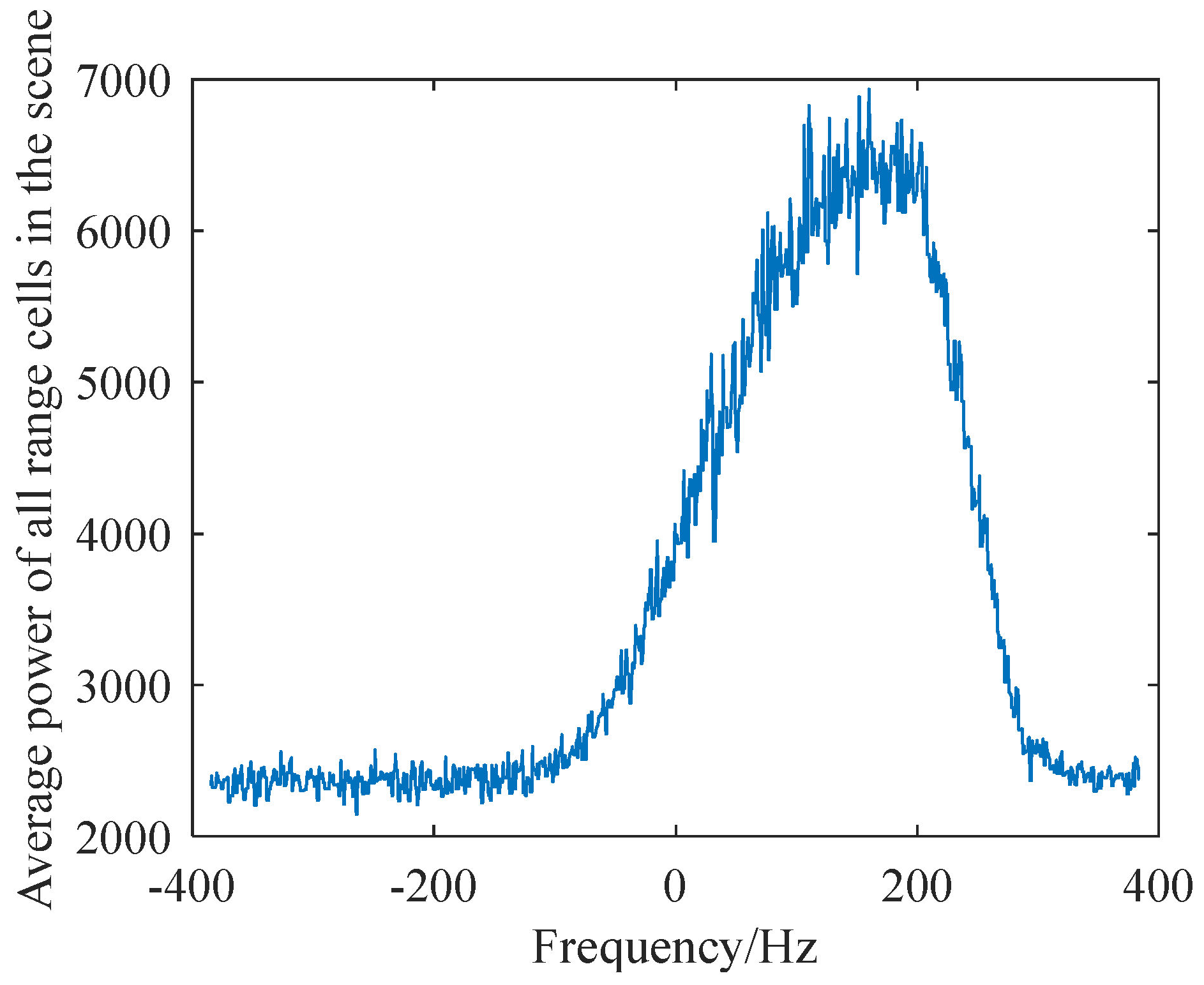
After obtaining the Doppler spectrum of the echo, the average power spectrum of all range units in the scene is calculated. The results are shown in
Figure 12. The estimated value of the Doppler center frequency can be calculated to be 81.90hz. The theoretical value of the SAR Doppler center frequency in the case of the frontal view is 0. If the Doppler center frequency is not estimated directly, the Doppler center is 0 for the construction of the approximate observation operator. The above error will cause the quality of the sparse reconstruction results to decrease.
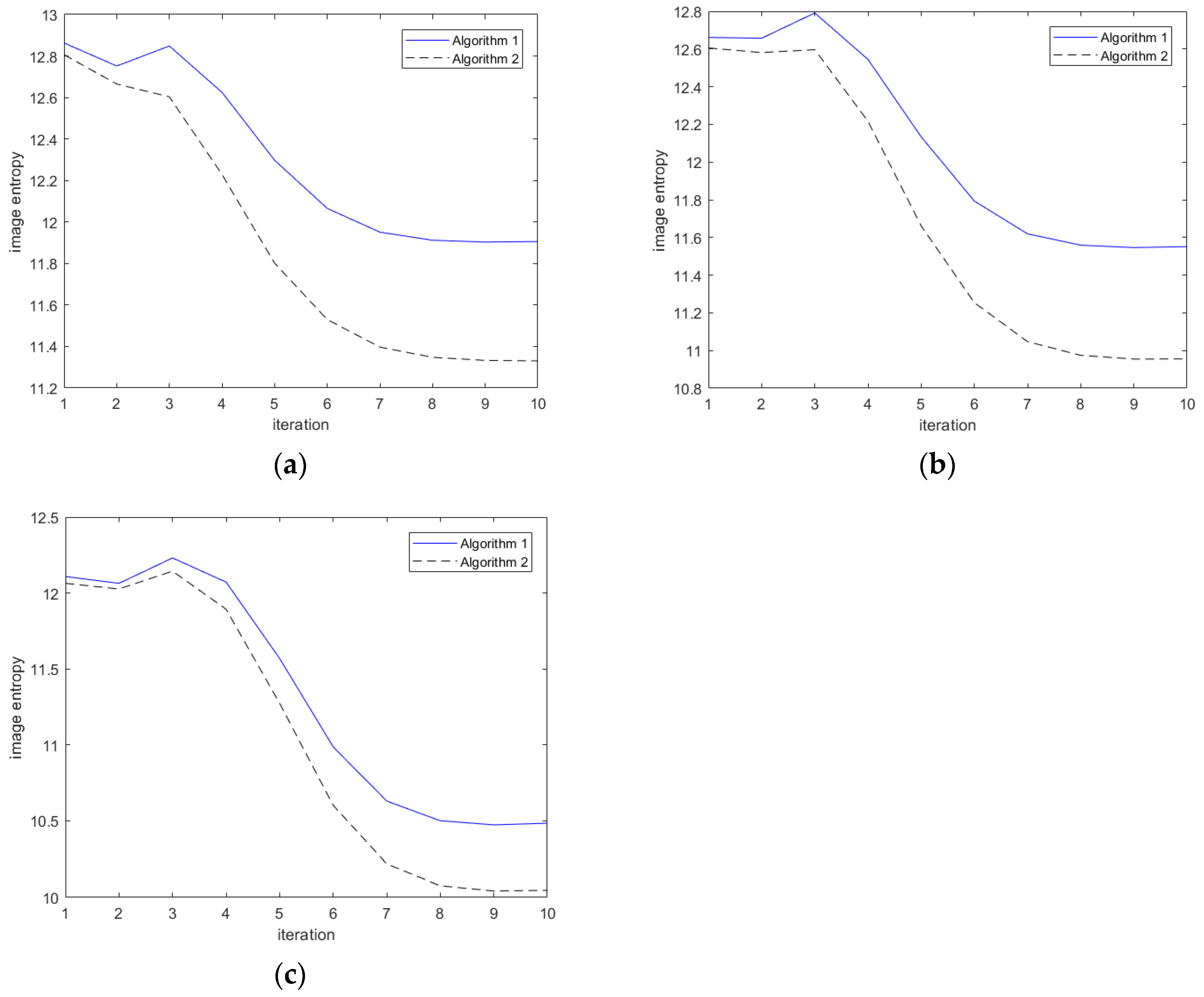
The above images are judged by the entropy of the image. The entropy of the image is expressed as the average number of bits of the gray level set of the image, which describes the average information amount of the image source. It is generally believed that a smaller entropy value of the image indicates a better focusing quality of the SAR image.
The change in the entropy value of each method in 10 iterations is shown in
Figure 13. The final entropy value of the image convergence of each algorithm under each sampling rate after 10 iterations is shown in
Table 3.
Figure 13 and
Table 3 show that, under the same undersampling rate, the initial entropy value of the image of Algorithm 2 and the final entropy value of image convergence are lower than those of Algorithm 1. The results show that Algorithm 2 has a better sparse reconstruction effect than Algorithm 1. Although Algorithm 1 can reconstruct the scene, it does not consider the impact of the non-ideal motion of the carrier on the Doppler center. Therefore, the sparse reconstruction effect is affected, and the target position in the scene is offset. This paper selects the sparse autofocus algorithm proposed in a previous study [
16] to compensate for the phase error in SAR data during the experiment. However, the sparse reconstruction effect cannot be further improved due to the errors in the parameters of the approximate observation operator itself, and the inherent errors of the algorithm model cannot be compensated. For Algorithm 2 proposed in this paper, the approximate observation operator matches the mathematical model of the actual imaging algorithm better due to the correction of the deviation of the Doppler parameter. The accurate Doppler center frequency improves the signal-to-noise ratio and image resolution, and the corresponding Algorithm 2 has a better sparse reconstruction effect. The iterative entropy from the image and the converged final entropy of Algorithm 2 are significantly better than those of Algorithm 1.


