A Robust Chronic Kidney Disease Classifier Using Machine Learning

Abstract

Clinical support systems are affected by the issue of high variance in terms of chronic disorder prognosis. This uncertainty is one of the principal causes for the demise of large populations around the world suffering from some fatal diseases such as chronic kidney disease (CKD). Due to this reason, the diagnosis of this disease is of great concern for healthcare systems. In such a case, machine learning can be used as an effective tool to reduce the randomness in clinical decision making. Conventional methods for the detection of chronic kidney disease are not always accurate because of their high degree of dependency on several sets of biological attributes. Machine learning is the process of training a machine using a vast collection of historical data for the purpose of intelligent classification. This work aims at developing a machine-learning model that can use a publicly available data to forecast the occurrence of chronic kidney disease. A set of data preprocessing steps were performed on this dataset in order to construct a generic model. This set of steps includes the appropriate imputation of missing data points, along with the balancing of data using the SMOTE algorithm and the scaling of the features. A statistical technique, namely, the chi-squared test, is used for the extraction of the least-required set of adequate and highly correlated features to the output. For the model training, a stack of supervised-learning techniques is used for the development of a robust machine-learning model. Out of all the applied learning techniques, support vector machine (SVM) and random forest (RF) achieved the lowest false-negative rates and test accuracy, equal to $99.33\%$ and $98.67\%$, respectively. However, SVM achieved better results than RF did when validated with 10-fold cross-validation.

1. Introduction

Kidneys are vital organs that keep track of salt, potassium, and caustic substances within the human body [1], and consist of 5 L of blood. If the kidneys cease to function normally, squanders form in the blood. As a result, this blood is converted into 9–10 L of a toxic fluid containing urea and creatinine in just 2–3 days. This condition is called chronic kidney disease (CKD). People possessing medical conditions such as diabetes, hypertension, cardiac disorder, or other kidney problems are more likely to have chronic kidney disease, while some kidney diseases are hereditary. Moreover, kidney disease becomes more likely as a person ages [2].

Individuals aged 65 or older ($38.1\%$) are more prone to CKD than individuals in the ranges of 45–64 ($12.4\%$) and 18–44 ($6\%$) years are, and women are more prone to CKD ($14.3\%$) than men ($12.4\%$) are [3]. According to the current medical statistics, CKD affects a stunning $10\%$ of the world’s population. In 2005, approximately 38 million deaths out of the 58 million total fatalities that occurred in that year were caused by CKD [4]. COVID-19 was found in $4.09\%$ of CKD patients ($193/4716$ patients), but only in a percentage equal to $0.46\%$ of the general population (5195/1,125,574). The crude mortality rate among COVID-19-positive CKD patients was $44.6\%$ ($86/193$), compared to $4.7\%$ ($215/4523$) in COVID-19-negative CKD patients [5]. When analyzing cases requiring renal replacement therapy (RRT), $55\%$ of the patients had Stage 5 CKD, and $30\%$ had Stage 3 CKD. In addition, $70\%$ of patients who required RRT had a fatal outcome [6].

Healthcare practitioners employ two basic approaches for obtaining clear patient insights to detect kidney disease. Initially, blood and urine tests are used to determine if a person has CKD; a blood test can determine kidney function, also known as the glomerular filtration rate (GFR). If the GFR value equals 60, this indicates normal kidney function, while values between 15 and 60 mean the kidneys are substandard. Lastly, if the GFR value equals to 15 or less, this indicates kidney failure [2]. The second approach, the urinalysis test, looks for albumin that can flow into the urine if the kidneys are not properly working.

The significance of early diagnosis is very high for reducing the mortality rate in CKD patients. A late diagnosis of this condition often leads to renal failure, which provokes the need for dialysis or kidney transplantation [7]. Because of the growing number of CKD patients, a paucity of specialized physicians has led to high costs of diagnosis and treatment. Particularly in developing countries, computer-assisted systems for diagnostics are needed to assist physicians and radiologists in making diagnostic judgments [8].

In such a situation, for the early and efficient prognosis of the disease, computer-aided diagnosis can play a crucial part. Machine learning (ML), which is a subdomain of artificial intelligence (AI), can be used for the adept identification of an ailment. These systems are aimed to aid clinical decision makers in performing more accurate disease classification. This work proposes a refined CKD identification ML model trained using the UCI CKD dataset and supervised-learning techniques SVM and RF. For enhancing the model’s scalability, several steps, such as missing-value imputation, data balancing and feature scaling, were employed [9]. The chi-squared technique was also used for the feature selection methodology. In addition to this, ML-based performance boosting methods such as hyperparameter tuning were also used to tune the model using the best possible set of parameters. The efficiency of the proposed work in terms of the testing accuracy was compared with that of various other studies.

The rest of the paper is organized as follows. The related work and the novelty of our work are introduced in Section 2. Section 3 overviews the basic concepts, methods, algorithms, and used dataset that were utilized in this paper. Section 4 presents the research results, while Section 5 depicts the comparison between the proposed framework and others from the literature. Lastly, Section 6 outlines the conclusions and draws directions for future work.

2. Related Work

Different methods and techniques for the problem of chronic kidney disease classification have been proposed and employed in the literature. The proposed research takes into account the existing literature, and further contributes towards enhancing the currently achievable results in the field of chronic kidney disease prediction.

An ML-based disease classification system using the UCI CKD dataset was employed in [10]. Out of all implemented algorithms, random forest achieved the highest accuracy value. This study, however, did not consider outliers while imputing the missing numerical values. The model was also trained on imbalanced data, and no feature selection was performed. Other drawbacks are the absence of hyperparameter tuning and the fact that the model was not cross-validated. In [8], a set of ML algorithms for the development of the CKD classifier was implemented. Random forest achieved the best accuracy. However, no outlier considered imputation, and no data balancing and hyperparameter tuning were performed. In addition, the efficiency of the proposed model was not cross-validated.

The authors in [11] implemented a method based on both machine learning and deep learning. Specifically, out of all the implemented machine-learning algorithms, the SVM model had the highest accuracy. The imputation of the missing values, i.e., the outliers, was not considered in that study. However, this work utilized all the features present in the dataset in terms of the ML model training. Furthermore, another ML-based CKD classifier was developed in [12]. Again, the SVM model showed the highest testing set accuracy. As above, the imputation was implemented without considering the presence of outliers. Data balancing was not performed, while this work uses 12 features for building and training the ML model. Moreover, hyperparameter tuning to improve the model accuracy was not performed.

A healthcare support system based on machine learning for the prognosis of the CKD was introduced in [13]. The decision tree (DT) algorithm showed the highest accuracy. However, an inconsistency lay with the imputation of the missing data that was performed without considering the presence of outliers; in addition, no data balancing was performed. This study uses the correlation-based feature selection (CFS) method for feature selection. This study developed the proposed model with the use of 15 features; however, again, no hyperparameter tuning was performed. Lastly, machine-learning and deep-learning techniques were employed for the construction of an ailment classifier in [14]. The highest accuracy was achieved by the random forest algorithm. Similarly, the imputation was implemented without considering outliers in the numerical features, and the training was utilized on the imbalanced dataset. Hyperparameter tuning was not performed while training the model, and the developed models were not cross-validated.

After investigating the contributions of different researchers for the prediction of CKD in the literature, the following research gaps were identified:

(i)

None of the literature papers considered the presence of outliers in the numerical features during the data preprocessing phase. Due to this, the imputed values in such features are prone to deviating from the overall central tendency.

(ii)

The majority of the literature trained their models on imbalanced data, which lead to a biased model.

(iii)

The majority of the literature did not perform hyperparameter tuning to boost the model’s efficacy.

(iv)

Most of the literature did not consider a feature selection method to identify the most relevant and optimal number of features. Hence, in this case, the models were fed with a set of extraneous features. Economically, this increases the cost of the medical examination of this renal ailment.

(v)

This work focuses on the cost-efficient and accurate medical examination of CKD while using fewer than 10 features for the model training and classification of the condition.

3. Methodology

A step-by-step and rather meticulous description of the methodology employed in this work is outlined in the following section.

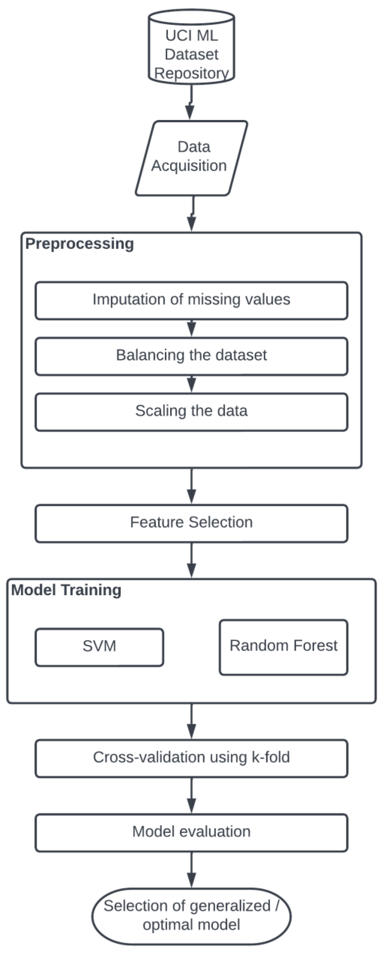
3.1. Proposed System

An accurate system for the identification of chronic kidney disease using a robust model is proposed in this work. An ML-based approach was utilized for the development of an effective and accurate prediction model. Figure 1 illustrates a schematic representation that depicts the different stages of the proposed system.

3.2. Dataset

The dataset used for performing the model training in this work was acquired from the UCI ML repository [15]. This repository is one of the most reliable and used dataset sources for researching and implementing machine-learning algorithms. There are 400 records and 25 features in this particular collection, including class attributes such as CKD and NOTCKD, indicating the status of chronic kidney disease in the patient. This dataset includes 14 categorical and 11 numerical features. This dataset had a considerable number of missing values, with only 158 records having no missing values. There was a significant imbalance between the presence of 250 CKD ($62.5\%$) and 150 NOTCKD ($37.5\%$) observations.

Table 1. Attribute descriptions.

Attributes	Information
Age	Discrete integer values
Blood pressure (BP)	Discrete integer values
Specific gravity (SG)	Discrete integer values
Albumin (AL)	Nominal values (0, 1, 2, 3, 4, 5)
Sugar (SU)	Nominal values (0, 1, 2, 3, 4, 5)
Red blood cells (RBC)	Nominal values (normal, abnormal)
Pus cell (PC)	Nominal values (normal, abnormal)
Pus cell clumps (PCC)	Nominal values (present, not present)
Bacteria (BA)	Nominal values (present, not present)
Blood glucose (BGR)	Numerical values in mg/dL
Blood urea (BU)	Numerical values in mg/dL
Serum creatinine (SC)	Numerical values
Sodium (SOD)	Numerical values in mEq/L
Potassium (POT)	Numerical values in mEq/L
Hemoglobin (HEMO)	Numerical values in gms
Packed cell volume (PCV)	Numerical values
White blood cell count (WC)	Discrete integer values
Red blood cell count (RC)	Numeric values
Hypertension (HTN)	Nominal values (yes, bo)
Diabetes mellitus (DM)	Nominal values (yes, no)
Coronary artery disease (CAD)	Nominal values (yes, no)
Appetite (APPET)	Nominal values (good, poor)
Pedal edema (PED)	Nominal values (yes, no)
Anemia (ANE)	Nominal values (yes, no)
Classification (CLASS)	Nominal Values (CKD, not CKD)

displays the descriptions and essential information of the features.

3.3. Data Preprocessing

The CKD dataset comprises outliers and missing data that need to be cleaned up during the preprocessing stage. There was also an imbalance in the dataset that caused a bias in the model. The preprocessing stage consists of the estimation and imputation of missing values, noise removal such as outliers, and dataset balancing [16]. To perform the preprocessing steps, the categorical features in the dataset were initially replaced with dummy values such as 0 and 1 using a label-encoding technique.

The dataset contained several missing values, with only 158 patients’ records contained no missing values. In the preprocessing stage, these missing data were mainly imputed using two central tendency values. The missing values in the numerical features with no outliers were imputed using the mean ($\overline{\mathrm{x}}$) of the respective column. In the case of numerical features with outliers, the central tendency mode ($Mo$) was used for the imputation of the missing values, as imputation with $\overline{\mathrm{x}}$ in such features deviates the imputed value from the average feature value range due to the presence of the outlier [17]. For all the missing values in the categorical features, $Mo$ was used for the imputation.

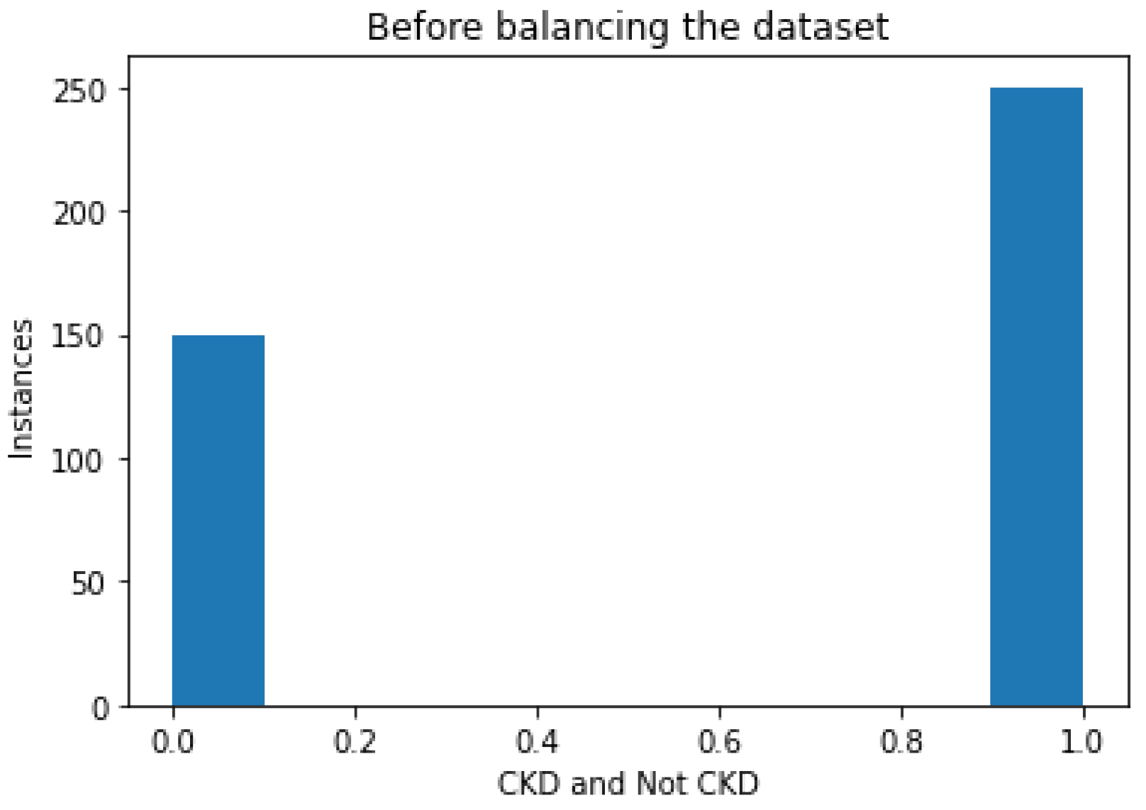
Following imputation, the data were balanced. The dataset consisted of 250 instances of patients with this disorder, and 150 instances of patients not having the disorder, as depicted in Figure 2; this type of distribution caused the bias in the model. Hence, balancing the dataset was performed in the preprocessing stage.

The balancing of the dataset was performed with the use of an oversampling method. Rather than the random generation of data points in terms of balancing, a SMOTE-based oversampling algorithm was employed in this work [18]; the SMOTE algorithm workflow is illustrated in Figure 3. To be more specific, a random sample from the minority class was initially selected, and k nearest neighbors were identified. Then, the vector between the selected data point and the neighbor was identified. This vector was multiplied by any random number from 0 to 1. Lastly, after we had added this vector to the current data point, the synthetic data point was obtained.

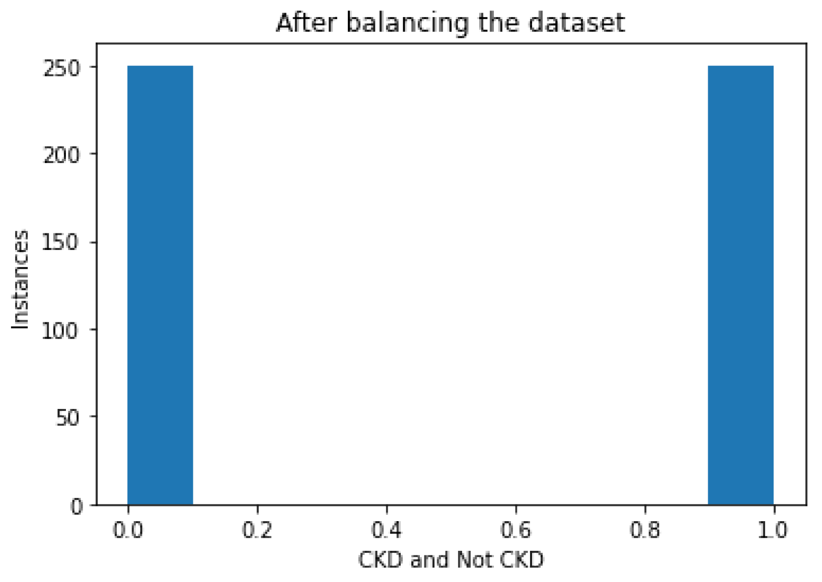
Figure 4 illustrates a bar diagram that depicts the instances of CKD and NOTCKD in the dataset after the balancing phase using the SMOTE algorithm.

After balancing the dataset, the next step was to remove noise such as outliers present in the dataset. For this purpose, feature scaling was employed, which was implemented with the use of MinMaxScaler [19].

3.4. Feature Selection

Each trained machine-learning classifier requires feature selection, since the results may be impacted if extraneous features are used while training the model [20].

The correlation of independent features with the target class is determined using the chi-squared feature selection approach [21]. With its robustness in handling categorical data and its property of making no assumptions in the distribution of the data, the chi-squared test was chosen for the purpose of feature selection in this work. Additionally, in this test, the target class and each independent feature’s chi-squared value were computed.

Features with better chi-squared scores were selected for the prediction because model prediction could thus be enhanced. This test is based on hypothesis testing, and the null hypothesis states that the features are independent of one another. The chi-squared score was calculated with the use of Equation (1):

$${\chi }_f^2=\sum \frac{{(O_i-E_i)}^2}{E_i}$$

(1)

where f denotes degrees of freedom, O denotes the observed values, and E denotes the expected values.

For the null hypothesis to be rejected, a high chi-squared score is required. Therefore, a high chi-squared value denotes a feature with great sustainability. The top 9 features based on the chi-squared test along with their chi-squared scores are shown in

Table 2. Selected features and their chi-squared scores.

Feature	Chi-Squared Score
Specific gravity	28.524025
Albumin	76.082337
Sugar	33.677092
Pus cell clumps	42.000000
Hypertension	144.042405
Diabetes mellitus	137.000000
Coronary artery disease	34.000000
Pedel edema	76.000000
Anemia	60.000000

.

Figure 5 illustrates the bar graph plot of the chi-squared values of all the features presented in the dataset. We noticed higher values of albumin, diabetes mellitus, coronary artery disease, pedel edema, and anemia, as identified from the corresponding dataset.

3.5. Training and Test Split

The preprocessed dataset containing the selected features was split for model training and evaluation into two parts: training and testing. The training set contained $70\%$ of the records in the preprocessed dataset, whereas the testing set contained $30\%$ of the records. Furthermore, the total number of training samples used was 350.

3.6. Model Training

During the model training phase, the two most efficient machine-learning classifiers, namely support vector machine (SVM) and random forest (RF), were trained using the preprocessed and cleaned dataset. During model training, the hyperparameters for the two algorithms were tuned to boost the performance.

3.6.1. Hyperparameter Tuning

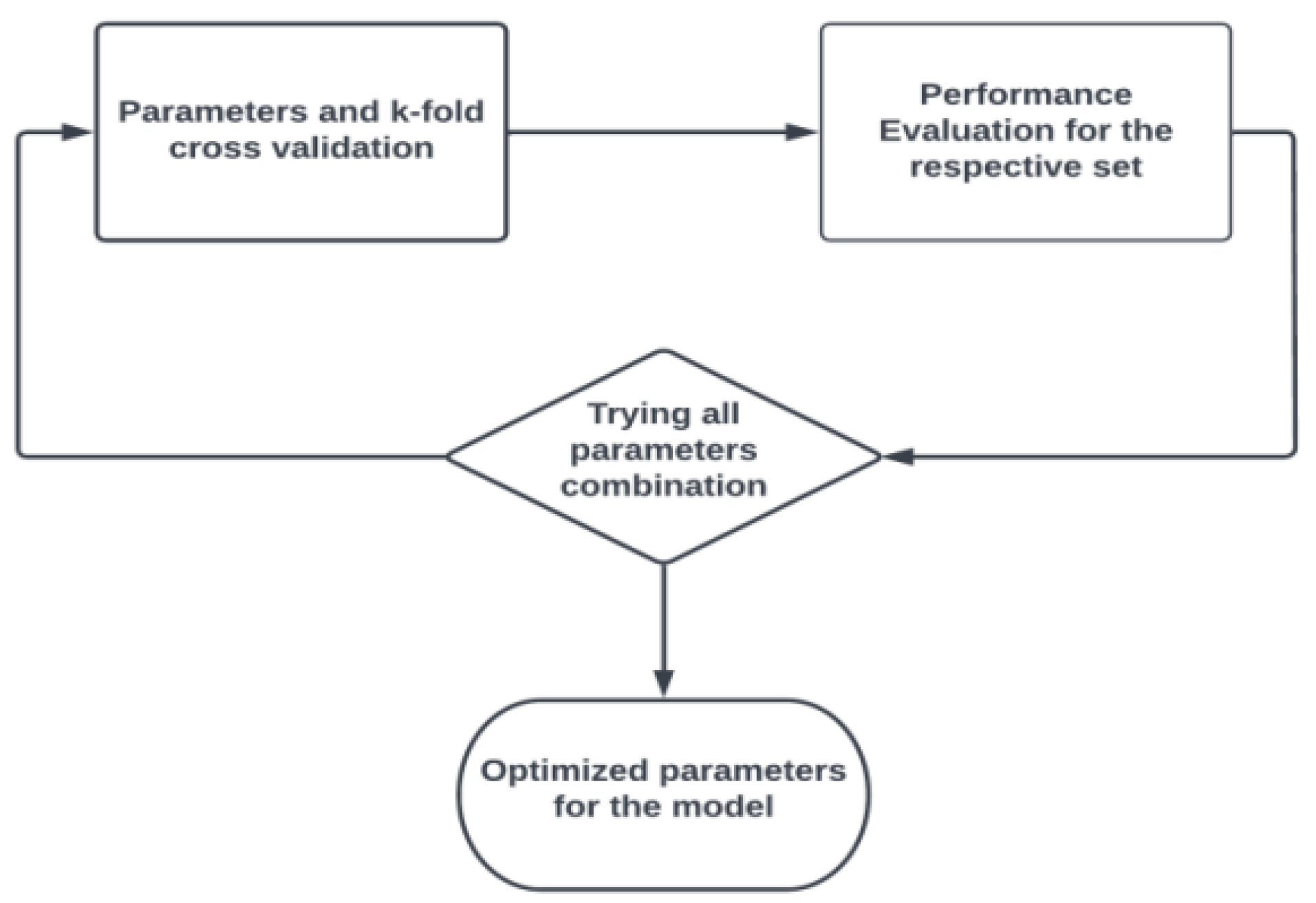
Hyperparameters (HPs) are the set of parameters used to define the model’s design and architecture [22]. For an accurate model design, different arrangements of HPs were investigated while preparing the model, and the best arrangement was chosen to characterize the model design. This method of boosting the model accuracy is referred to as hyperparameter tuning (HPT). To find the optimal model design, a search is performed through the various possible sets of HPs.

In this work, regarding HPT, the method of GridSearchCV was implemented in order to find the optimal values of the selected HP values. The workflow of GridSearchCV for the selection of HPs is illustrated in Figure 6.

3.6.2. Support Vector Machine

The SVM is a widely used and adopted supervised ML algorithm utilized for problems such as classification [23]. The SVM works with the generation of an optimal line known as a hyperplane. The function of this hyperplane is to segregate a given number of dimensions into more than one. As a result, whenever a new data point is to be evaluated, it can be assigned to the most appropriate category. The SVM chooses the point along with a vector representing the extremes for the generation of hyperplanes. These extremes are referred to as support vectors, which is why this algorithm is referred to as SVM [24].

Furthermore, the SVM can be characterized by two HPs, i.e., C and Kernel [23]. The C parameter penalizes a misclassified point in a dataset. A lower value of C implies a low penalty for misclassification, showing that a decision boundary with a relatively higher margin is chosen at the cost of a greater number of wrong classifications.

On the other hand, Kernel is a measure of similarity. This resemblance implies a degree of closeness. Common values of Kernel HP are linear and rbf. Specifically, the values chosen by GridSearchCV were {C: 14, Kernel: rbf}.

rbf stands for radial basis function, and due to its resemblance to the Gaussian distribution, it is among the most commonly utilized types of kernelization. The similarity or degree of proximity between two points, $x_1$ and $x_2$, is calculated using the RBF Kernel function. This Kernel’s mathematical representation is presented in Equation (2).

$$k(x_1,x_2)=exp(-\frac{\left|\right|x_1-x_2{\left|\right|}^2}{2{\sigma }^2})$$

(2)

where $\sigma$ denotes variance, and $\left|\right|x_1-x_2\left|\right|$ is the Euclidean distance between two points, $x_1$ and $x_2$.

3.6.3. Random Forest

The RF constitutes an ensemble method that resembles the closest neighbor predictor in several ways [25]. The divide-and-conquer strategy of ensembles is employed to boost performance. This follows the concept of combining several weak learners to form a robust learner. In the case of RF, the DT algorithm acts as a weak learner that is to be aggregated, and repeatedly divides the dataset using a criterion that optimizes the separation of the data, thus producing a structure resembling a tree. The predictions of unknown inputs after training are calculated using Equation (3) [26].

$$f^{\prime }=\frac{1}{B}\sum _{b=1}^B{f}_b\left(x^{\prime }\right)$$

(3)

where B is the optimal number of trees.

The uncertainty $\sigma$ of the prediction is depicted in Equation (4).

$$\sigma =\sqrt{\frac{{\sum }_{b=1}^B{(f_b\left(x^{\prime }\right)-f^{\prime })}^2}{B-1}}$$

(4)

HPs that can be used to define the random forest start with a criterion. This parameter is used to estimate the grade of the split. The information gain to be performed for this parameter is channelized using either $entropy$ or $gini$.

$min\_samples\_leaf$ signifies the minimal sample size that must be present in the leaf node after splitting the node, while $min\_samples\_split$ stands for the number of observations required for splitting it. Another important HP is the number of estimators ($n\_estimators$), which signifies how dense the random forest is. Moreover, it depicts the number of trees that are to be used to construct the random forest.

The next vital HP in RF is the number of jobs ($n\_jobs$), which indicates the restrictions on using the processor, if any. A value that equals $-1$ indicates the presence of no restrictions on the use of the processor, whereas a value equaling 1 shows that only one processor is to be used.

Random state is a numerical parameter representing the random combination of the training and test split. The values chosen by GridSearchCV were {$criterion$: $gini$, $min\_samples\_leaf$: 1, $min\_samples\_split$: 3, $n\_estimators$: 16, $n\_jobs$: 1, $random\_state$: 123}.

4. Results

To establish the effectiveness of the proposed models, the different performance parameters of accuracy, confusion matrix, precision, recall, F1 score, Cohen’s kappa coefficient, ROC curve, and cross-validation score were utilized as shown in

Table 3. Classification report of the trained models, selected features, and their chi-squared scores.

	Support Vector Machine				Random Forest
	Precision	Recall	F1 Score	Support	Precision	Recall	F1 Score	Support
CKD	0.99	1.00	0.99	76	0.97	1.00	0.99	76
NOT-CKD	1.00	0.99	0.99	74	1.00	0.97	0.99	74
Macro avg	0.99	0.99	0.99	150	0.99	0.99	0.99	150
Weighted avg	0.99	0.99	0.99	150	0.99	0.99	0.99	150

,

Table 4. Confusion matrix for the trained models.

	Support Vector Machine		Random Forest
	Positive	Negative	Positive	Negative
Positive	76	0	76	0
Negative	1	73	2	72

,

Table 5. AUC-ROC, log loss value, and Cohen’s kappa coefficient.

	Support Vector Machine	Random Forest
AUC-ROC	0.9932	0.9864
Log loss value	0.2303	0.4605
Cohen’s kappa	0.9867	0.9733

and

Table 6. Foldwise score of the trained models.

Support Vector Machine		Random Forest
Folds	Accuracy (%)	Folds	Accuracy (%)
2	98	2	96.9
3	98	3	97.7
4	98	4	97.7
5	98	5	97.7
6	98	6	97.4
7	98	7	98
8	98	8	97.4
9	98	9	98
10	97.8	10	98

and Figure 7 and Figure 8 [27]. Classifier accuracy is the ratio of successfully identified cases to the total number of instances [28]. Recall signifies the model’s efficacy in terms of identification of positive samples, and precision signifies the model’s efficacy in identifying the quality of positive cases detected by the classifier [29,30]. The model’s effectiveness in terms of both recall and precision is measured by their calculated geometric mean, known as the F1 score. The macro average is the mean of scores, and the weighted average uses the added weight of the count to the scores. The support is the count of records belonging to a specific class in the test dataset. The log loss value is the score of the cross-entropy of the error, and Cohen’s kappa coefficient is a measure of the inter-rating.

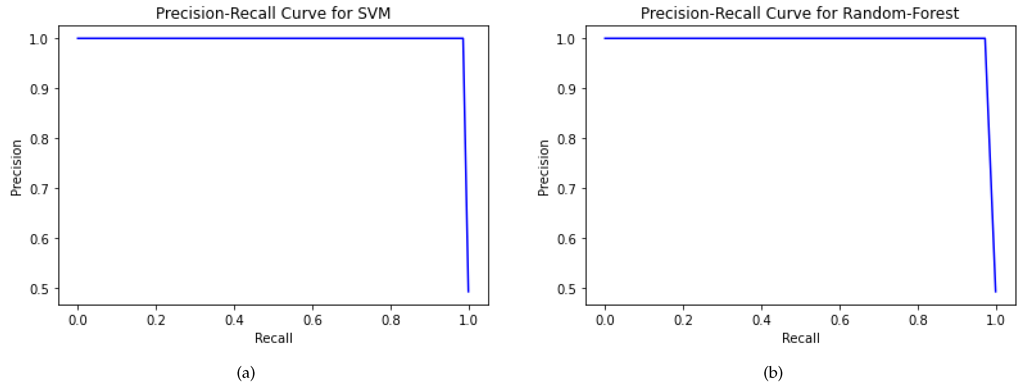
The PR curve is a plot drawn between true positives and false positives, used to gauge a classifier’s sensitivity [29]. The area under the curve (AUC) ranges from 0 to 1 [31]. The higher the AUC score is, i.e., closer to 1, the higher the model’s efficacy is. The testing set accuracy of SVM and RF is $99.33\%$ and $98.67\%$, respectively.

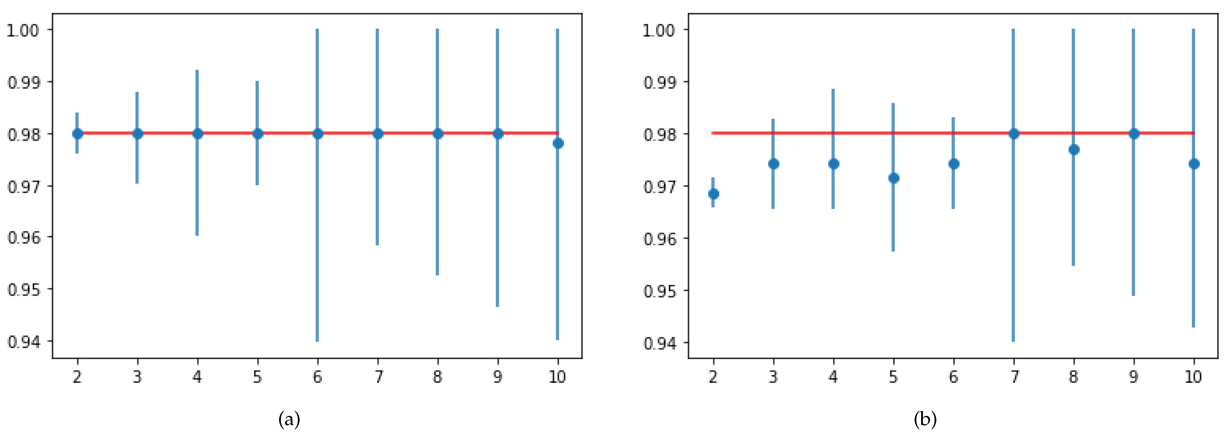
The trained model’s generalization capability can be validated using the 10-fold cross validation score. SVM and RF showed the same cross-validation score, equal to $98\%$. However, in terms of test accuracy and recall score, SVM was more robust than RF. The 10-fold cross-validation of SVM and RF is represented in Figure 8.

5. Comparative Analysis

The comparative analysis presented in

Table 7. Comparative analysis of the various studies.

Reference Number	Method	Accuracy (%)
Senan et al. [8]	Random forest	100
Revathy et al. [10]	Random forest	99.16
Chittora et al. [11]	Support vector machine	98.46
Reshma et al. [12]	Support vector machine	96
Cahyani et al. [13]	C4.5 (decision tree)	97.5
Shankar et al. [14]	Random forest	99
Proposed model–SVM		99.33

presents the accuracy achieved in various studies by various authors for CKD classification. The proposed model in our study showed great efficacy in terms of CKD classification with a test accuracy value equal to $99.33\%$ in SVM, and k-fold cross validation score equal to $98\%$ [32]. This generalized result compared to that of other works is attributed to several methodologies adopted in this work, such as appropriate data imputation, data balancing, feature scaling, chi-squared-based feature selection, and HPT using GridSearchCV.

Initially, the appropriate data imputation was performed while taking into consideration the outliers present in the numerical features. For the class of numerical features containing outliers, the imputation was performed using the $Mo$ (mode) of the respective feature. None of the other corresponding related works considered the outliers that were present in the dataset during the time of imputation.

Second, a major performed step was data balancing with the use of the SMOTE algorithm. The majority of the works listed in the table trained their models on imbalanced data, thus causing a bias in the model. Third, a set of 9 highly correlated features were extracted using the chi-squared score.

A major part of the listed works did not consider feature selection, leading to feeding the classifier with extraneous and irrelevant features. Additionally, the accuracy boosting practice of HPT was performed to find the set of optimal values for the model using GridSearchCV. Lastly, the model’s generalization test was performed using 10-fold cross validation, showing a promising score equal to $98\%$.

6. Conclusions and Future Work

A thorough investigation of the performance of various methods regarding chronic kidney disease (CKD) identification was initially performed in this work. Following this investigation, appropriate data preprocessing steps were performed to handle flaws in the CKD dataset such as missing values, imbalanced data, and the presence of outliers; then, an effective SVM model was created by tuning the hyperparameters. The nine most important features for improving the accuracy and other performance parameters were selected. When the model was evaluated on the testing set containing 150 records, it showed promising results, with just $0.67\%$ false negative rates. This method can have real-time application for the accurate diagnosis of the fatal renal condition of chronic kidney disease. Early diagnosis can be performed with the help of this application, eventually leading to a reduction in the mortality rate.

The main novelty of the proposed paper lies with the features used for identification. On the one hand, highly advanced and expensive tests for CKD detection are difficult in rural areas, and on the other hand, the medical examination of the features used in this work is generally available even in rural area’s pathology laboratories.

Diagnoses based on MRI and CT scan methods are not always accurate, incur high costs, and are time-consuming. The proposed method had a low false-positive rate and zero false negatives. A diagnosis using the proposed method needs fewer inputs, which reduces the test cost and prediction time. Hence, for rural areas, diagnosis using the proposed method is more feasible as compared to that with conventional MRI and CT scan methods.

Lastly, a possible future scope lies with the achievement of similar or even higher accuracy values with fewer features with the aim to reduce the cost of medical diagnosis even more. For the same purpose of feature selection, rather than classical. statistical methods, hybrid feature selection techniques can also be employed to extract a more general and appropriate set of features. This work can only predict the absence or the presence of the disease. Hence, a more intense dataset can be employed to predict the severity stage of the disease of any patient.

References

- National Kidney Foundation Inc. How Your Kidneys Work. Available online: https://www.kidney.org/kidneydisease/howkidneyswrk (accessed on 4 November 2022).
- National Institute of Diabetes and Digestive and Kidney Diseases (NIDDK). Chronic Kidzney Disease (CKD). Available online: https://www.niddk.nih.gov/health-information/kidney-disease/chronic-kidney-disease-ckd (accessed on 4 November 2022).
- Centers for Disease Control and Prevention. In Chronic Kidney Disease in the United States; 2021. Available online: https://www.cdc.gov/kidneydisease/publications-resources/CKD-national-facts.html (accessed on 4 November 2022).
- Levey, A.S.; Atkins, R.; Coresh, J.; Cohen, E.P.; Collins, A.J.; Eckardt, K.U.; Nahas, M.E.; Jaber, B.L.; Jadoul, M.; Levin, A.; et al. Chronic Kidney Disease as a Global Public Health Problem: Approaches and Initiatives—A Position Statement from Kidney Disease Improving Global Outcomes. Kidney Int. 2007, 72, 247–259. [Google Scholar] [CrossRef] [PubMed] [Green Version]
- Gibertoni, D.; Reno, C.; Rucci, P.; Fantini, M.P.; Buscaroli, A.; Mosconi, G.; Rigotti, A.; Giudicissi, A.; Mambelli, E.; Righini, M.; et al. COVID-19 Incidence and Mortality in Non-Dialysis Chronic Kidney Disease Patients. PLoS ONE 2021, 16, e0254525. [Google Scholar] [CrossRef] [PubMed]
- Pawar, N.; Tiwari, V.; Gupta, A.; Bhargava, V.; Malik, M.; Gupta, A.; Bhalla, A.K.; Rana, D.S. COVID-19 in CKD Patients: Report from India. Indian J. Nephrol. 2021, 31, 524. [Google Scholar]
- Garcia, G.G.; Harden, P.; Chapman, J. The Global Role of Kidney Transplantation. Kidney Blood Press. Res. 2012, 35, 299–304. [Google Scholar] [CrossRef] [PubMed] [Green Version]
- Senan, E.M.; Al-Adhaileh, M.H.; Alsaade, F.W.; Aldhyani, T.H.H.; Alqarni, A.A.; Alsharif, N.; Uddin, I.; Alahmadi, A.H.; Jadhav, M.E.; Alzahrani, M.Y. Diagnosis of Chronic Kidney Disease Using Effective Classification Algorithms and Recursive Feature Elimination Techniques. J. Healthc. Eng. 2021, 2021, 1004767. [Google Scholar] [CrossRef]
- Das, D.; Nayak, M.; Pani, S.K. Missing Value Imputation—A Review. Int. J. Comput. Sci. Eng. 2019, 7, 548–558. [Google Scholar] [CrossRef]
- Revathy, S.; Bharathi, B.; Jeyanthi, P.; Ramesh, M. Chronic Kidney Disease Prediction Using Machine Learning Models. Int. J. Eng. Adv. Technol. 2019, 9, 6364–6367. [Google Scholar] [CrossRef]
- Chittora, P.; Chaurasia, S.; Chakrabarti, P.; Kumawat, G.; Chakrabarti, T.; Leonowicz, Z.; Jasiñski, M.; Jasinski, L.; Gono, R.; Jasinska, E.; et al. Prediction of Chronic Kidney Disease—A Machine Learning Perspective. IEEE Access 2021, 9, 17312–17334. [Google Scholar] [CrossRef]
- Reshma, S.; Shaji, S.; Ajina, S.R.; Priya, S.R.V.; Janisha, A. Chronic Kidney Disease Prediction using Machine Learning. Int. J. Eng. Res. Technol. 2020, 9, 548–558. [Google Scholar] [CrossRef]
- Cahyani, N.; Muslim, M.A. Increasing Accuracy of C4.5 Algorithm by Applying Discretization and Correlation-based Feature Selection for Chronic Kidney Disease Diagnosis. J. Telecommun. 2020, 12, 25–32. [Google Scholar]
- Shankar, S.; Verma, S.; Elavarthy, S.; Kiran, T.; Ghuli, P. Analysis and Prediction of Chronic Kidney Disease. Int. Res. J. Eng. Technol. 2020, 7, 4536–4541. [Google Scholar]
- UCI Machine Learning Repository. Chronic Kidney Disease Dataset. Available online: https://archive.ics.uci.edu/ml/datasets/chronic_kidney_disease (accessed on 4 November 2022).
- Kotsiantis, S.; Kanellopoulos, D.; Pintelas, P. Handling Imbalanced Datasets: A Review. GESTS Int. Trans. Comput. Sci. Eng. 2006, 30, 25–36. [Google Scholar]
- Audu, A.; Danbaba, A.; Ahmad, S.K.; Musa, N.; Shehu, A.; Ndatsu, A.M.; Joseph, A.O. On The Efficiency of Almost Unbiased Mean Imputation When Population Mean of Auxiliary Variable is Unknown. Asian J. Probab. Stat. 2021, 15, 235–250. [Google Scholar] [CrossRef]
- Chawla, N.V.; Bowyer, K.W.; Hall, L.O.; Kegelmeyer, W.P. SMOTE: Synthetic Minority Over-sampling Technique. J. Artif. Intell. Res. 2002, 16, 321–357. [Google Scholar] [CrossRef]
- Jain, Y.K.; Bhandare, S.K. Min Max Normalization Based Data Perturbation Method for Privacy Protection. Int. J. Comput. Commun. Technol. 2011, 2, 45–50. [Google Scholar] [CrossRef]
- Guyon, I.; Elisseeff, A. An Introduction to Variable and Feature Selection. J. Mach. Learn. Res. 2003, 3, 1157–1182. [Google Scholar]
- Cai, L.J.; Lv, S.; Shi, K.B. Application of an Improved CHI Feature Selection Algorithm. Discret. Dyn. Nat. Soc. 2021, 2021, 9963382. [Google Scholar] [CrossRef]
- Elgeldawi, E.; Sayed, A.; Galal, A.R.; Zaki, A.M. Hyperparameter Tuning for Machine Learning Algorithms Used for Arabic Sentiment Analysis. Informatics 2021, 8, 79. [Google Scholar] [CrossRef]
- Zhang, Y. Support Vector Machine Classification Algorithm and Its Application. In International Conference on Information Computing and Applications; Springer: Berlin/Heidelberg, Germany, 2012; Volume 308, pp. 179–186. [Google Scholar]
- Swain, D.; Pani, S.K.; Swain, D. Diagnosis of Coronary Artery Disease using 1-D Convolutional Neural Network. Int. J. Recent Technol. Eng. 2019, 8. [Google Scholar]
- Biau, G. Analysis of a Random Forests Model. J. Mach. Learn. Res. 2012, 13, 1063–1095. [Google Scholar]
- Duan, H.; Liu, X. Lower C Limits in Support Vector Machines with Radial Basis Function Kernels. In Proceedings of the International Symposium on Information Technologies in Medicine and Education, Hokkaido, Japan, 3–5 August 2012; Volume 2, pp. 768–771. [Google Scholar]
- Liu, Y.; Zhou, Y.; Wen, S.; Tang, C. A Strategy on Selecting Performance Metrics for Classifier Evaluation. Int. J. Mob. Comput. Multimed. Commun. 2014, 6, 20–35. [Google Scholar] [CrossRef] [Green Version]
- Nishat, M.M.; Faisal, F.; Dip, R.R.; Nasrullah, S.M.; Ahsan, R.; Shikder, F.; Asif, M.A.; Hoque, M.A. A Comprehensive Analysis on Detecting Chronic Kidney Disease by Employing Machine Learning Algorithms. EAI Endorsed Trans. Pervasive Health Technol. 2021, 7, e1. [Google Scholar] [CrossRef]
- Swain, D.; Pani, S.K.; Swain, D. A Metaphoric Investigation on Prediction of Heart Disease using Machine Learning. In Proceedings of the 2018 International Conference on Advanced Computation and Telecommunication (ICACAT), Bhopal, India, 28–29 December 2018; pp. 1–6. [Google Scholar]
- Swain, D.; Pani, S.K.; Swain, D. An Efficient System for the Prediction of Coronary Artery Disease using Dense Neural Network with Hyper Parameter Tuning. Int. J. Innov. Technol. Explor. Eng. 2019, 8, 689–695. [Google Scholar]
- Swain, D.; Bijawe, S.S.; Akolkar, P.P.; Shinde, A.; Mahajani, M.V. Diabetic Retinopathy using Image Processing and Deep Learning. Int. J. Comput. Sci. Math. 2021, 14, 397–409. [Google Scholar] [CrossRef]
- Darapureddy, N.; Karatapu, N.; Battula, T.K. Research of Machine Learning Algorithms using K-Fold Cross Validation. Int. J. Eng. Adv. Technol. 2021, 8, 215–218. [Google Scholar]