A Measurement Compensation Method for Electrical Capacitance Tomography Sensors with Inhomogeneous Electrode Parameters

Abstract

An electrical capacitance tomography (ECT) sensor is an array capacitive sensor that is sensitive to the medium of the measured object and can be widely used in oil, natural gas, machinery and other industrial fields to solve the problem of multiphase fluid object parameter detection in industrial processes. However, ECT sensor uniformity defects need to be addressed. Aiming at the problem that the non-uniform electrode spacing angle affects the characteristics of the measured value of the actual ECT sensor, a method for compensating the measured value of the ECT sensor based on the assumption that the geometric factor is invariant is proposed. The simulated measurement value in the case of the tube and the measurement value of the actual sensor in the case of an empty tube and a full tube are to compensate the measurement value of the actual ECT. Experiments show that, without compensation, non-ideal sensor monitoring has large error, and, after compensation, it has a good effect and can be expected to perform satisfactorily in practical use.

1. Introduction

The hydraulic system and lubrication system of oil, natural gas and mechanical equipment and other pipelines or the fluid in the box are typical oil–water or gas–water two-phase flow objects. The fluid is often mixed with a variety of solid particles, and the phase interface is random. This makes the multiphase flow form complex and changeable, so the precise measurement, accurate calculation and effective prediction of its flow parameters and flow patterns have always been the focus and challenge of scientists and engineers in this field [1]. In recent years, the measurement method based on the capacitance method has been applied to the detection of two-phase flow parameters in oil and natural transportation pipelines and mechanical equipment. It has the characteristics of non-invasive and non-interfering flow field [2,3]. Among them, electrical capacitance tomography (ECT) technology is a kind of capacitance method. Its image can not only be used to realize the visual monitoring of the fluid in the pipe but can also be used to calculate the phase holdup [4,5,6], so the application prospects are significant.

In the late 1980s, Professor M. S. Beck of the University of Manchester Institute of Technology and his research team took the lead in researching industrial process tomography technology, and, in 1988, took the lead in developing the first device for detecting two-phase flow parameters. This electrical capacitance tomography (ECT) system was composed of an eight-electrode array [7]. Subsequently, a research group composed of the University of Manchester, the University of Leeds, the Morgan City Energy Technology Center of the US Department of Energy and some small- and medium-sized enterprises have conducted a great deal of research on the system, sensor optimization and application of capacitance tomography [8,9,10]. At the same time, Chinese universities and research institutes have also successively carried out research in this field. Tsinghua University, Tianjin University, Xi’an Jiaotong University, Institute of Engineering Thermophysics, Chinese Academy of Sciences and North China Electric Power University have all made breakthroughs in sensor electrode optimization, circuit design, reconstruction algorithms and industrial applications [11,12,13]. Wang Huaxiang [14,15], Liu Shi [16], Huang Zhiyao [17], Wang Baoliang [18], Hu Hongli [19,20,21] and other teams have devoted themselves to the research and development of electrical tomography technologies, such as electrical resistance tomography (ERT) and ECT, for many years and have conducted in-depth research in sensor design, signal acquisition, field sensitivity analysis and image reconstruction algorithms.

Since the introduction of ECT technology, researchers in many fields have studied its application. Among them, the application of ECT in multiphase flow parameter detection is one of the most active academic directions. In the following industrial occasions, the applications of ECT are widely studied: oil pipelines [22], wet gas separators, pneumatic powder conveying systems, gas/solid cyclones, circulating fluidized beds [23,24,25,26,27,28,29,30], fluidized bed dryer, etc. ECT-based multiphase flow parameter detection technology forms can be divided into two categories: (1) pure ECT-based detection technology, which only uses data obtained by ECT sensing or ECT images for multiphase flow parameter detection; (2) based on the technology of joint detection of ECT and other sensors (such as ultrasonic, differential pressure, capacitance, conductance sensors, etc.), this type of technology combines the advantages of ECT and other sensing technologies to realize the fusion measurement of multi-sensing information.

The ECT sensor is the key and core of the multiphase flow parameter measurement method based on ECT technology [31]. Practical applications show that ECT sensors are limited by many factors, such as process, cost and specific engineering requirements. There is a deviation between the geometric parameters of the actually manufactured ECT sensor and the design value, and, sometimes, this deviation may be very significant. When this non-ideal ECT sensor is used for imaging, the reconstructed image is not necessarily completely wrong. Usually, the pixel value in some areas of the image is too large, and the pixel value in some areas is too small. It may not be satisfactory for visual monitoring. However, such deviations can make flow pattern identification based on ECT measurements seriously erroneous because the geometrical deviations in the machining change the statistical characteristics of the measurement vector. However, the above problems of the ECT sensor have not been studied in depth.

In view of the above-mentioned scenario, this paper proposes a correction method for the measured value vector when there is a large deviation between the actual geometric parameters of the ECT sensor and the design value so as to ensure that the identification of flow patterns based on ECT measurements can be carried out smoothly. This study can not only provide a measurement correction method for researchers interested in ECT but also provide a more reliable technical tool for researchers working in flow dynamics and microfluidics.

2. Analysis of the Source of Geometric Inhomogeneity of ECT Sensor

This article takes an example of an ECT system for a natural gas pipeline. In this application, the sensor pipeline is required to be corrosion-resistant, wear-resistant and able to withstand high pressure. Therefore, when making the sensor, the tube is designed as PEEK material. In terms of sensor forming technology, two implementation schemes are designed in this paper:

2.1. Flexible Circuit (FPC) Process

First, the FPC patch of the ECT sensor electrode is pre-manufactured by the flexible circuit (flexible printed circuit, FPC) technology; then, the polyetheretherketone (PEEK) column material is processed by the cutting process to form the sensor pipe; finally, the FPC electrode patch is attached to the cut PEEK pipe. The main part of the ECT sensor finally formed by the FPC process is shown in Figure 1.

2.2. Sputtering Process

First, a cutting process is used to process the PEEK column material to form the sensor pipe, and the electrode groove is cut out on the sensor pipe; then, a layer of copper is completely sputtered on the cut sensor pipe; finally, the copper layer outside the electrode groove is removed by grinding to form electrode. The main flow of ECT sensor fabrication by sputtering process is shown in Figure 2.

Both of the above two sensor forming solutions have the advantages of mass production, simple process and strong achievability. Among them, the FPC process is simpler, but there may be problems of air bubbles, warpage and looseness when the FPC electrode sheet is glued to the sensor pipe, and the processing method needs to be optimized. The sputtering process is relatively complicated, but it can overcome the above-mentioned shortcomings of the FPC process. In addition to this, both processes have a common disadvantage—the electrode spacing angle may not be consistent: in the FPC process, the width of the FPC electrode sheet may not be exactly the same length as the pipe perimeter; this is because the PEEK column is being cut when forming a pipe, so the outer diameter of the actually processed pipe is larger than the design value and there will be a gap after the FPC electrode sheet is finally matched with the pipe (see Figure 1). This will result in uneven electrode spacing angle.

The sensitivity coefficient matrix of ECT is calculated numerically. At this time, the geometric model of the sensor is ideal: the electrode size is strictly consistent, and the electrode spacing is strictly equal. Obviously, such a strictly symmetrical structure makes the measured values of the sensor have obvious rules: when the sensitive area of the sensor is filled with a uniform medium or a rotationally symmetric medium at any angle, the same relative position (including adjacent, spaced n electrodes, relative positions) measurements are exactly equal. This paper defines this property of the sensor as the homogeneity of the sensor.

However, the actual manufacturing process often cannot make the sensor geometrically strictly symmetrical. In this case, non-uniformity will be manifested: even for a homogeneous medium or a symmetrical medium distribution, there is a large difference between the measured values of the sensor at the same relative position. Through practice, it has been found that this non-uniformity of the sensor may lead to errors in the identification of flow patterns based on the measured value vector because this non-uniformity will lead to the statistical characteristics between the elements of the measured value vector and the ideal situation presenting a major difference.

3. Measured Value Compensation of ECT Sensor Based on the Assumption of Invariant Geometric Factor

The measured values of the ECT sensor have obvious statistical characteristics, which are expressed as the standard deviation of each relative position measurement subset and the difference of the nth-order moment, which can be used for the construction of flow pattern characteristics. A “relative position measurement subset” of an ECT sensor measurement vector refers to a set of measurements of excitation–detection pairs that have the same spatial positional relationship. For the 12-electrode ECT sensor, this “spatial positional relationship” has six kinds of spatial positional relationships: adjacent, spaced n electrodes (n = 1, 2, …, 4) and relative. For example, measurements C_1,2 belong to the adjacent measurement subset, C_1,3 belong to the interval 1 electrode measurement subset and C_1,6 belong to the opposite measurement subset. According to this rule, it is not difficult to conclude that the relative measurement subsets each contain 6 elements, and the adjacent and spaced n-electrode subsets each contain 12 elements. The set of measured values of the electrode pairs in these six positional relationships is denoted as ${\mathit{P}}_n,n=1,2,\dots ,6$.

3.1. ECT Sensor Measurement Value Representation

Due to the excitation of our ECT system being an AC voltage source, the next equations will be demonstrated in phasor form. For ECT sensors, the measured value of sensor excitation pair i-j can be expressed as:

$$C_{i,j}={\dot{P}}_{i,j}/{\dot{V}}_{\mathrm{E}}^2=-\frac{1}{{\dot{V}}_{\mathrm{E}}}{\displaystyle {\int }_{\partial {\Omega }_j}\epsilon {\dot{E}}_i\cdot \mathrm{d}s}$$

(1)

Here, the concept of effective dielectric constant is introduced. The effective dielectric constant is defined here as: for any dielectric constant distribution, according to the integral median theorem, there is an effective dielectric constant $\tilde{\epsilon }$= ε(p), p∈∂Ω_j as a constant, such that:

$$\tilde{\epsilon }{\displaystyle {\int }_{\partial {\Omega }_j}{\dot{E}}_i\cdot \mathrm{d}s}={\displaystyle {\int }_{\partial {\Omega }_j}\epsilon {\dot{E}}_i\cdot \mathrm{d}s}$$

(2)

At this point, $\epsilon$ becomes a constant $\tilde{\epsilon }$, which can be removed from the integral sign of Equation (1). The electric field E_i is proportional to the amplitude of the excitation voltage, so the capacitance value shown in Equation (1) is a certain value. In fact, this is consistent with common sense: the capacitance value of a two-terminal capacitor is only related to its geometry and internal fill medium, not the excitation source. It should be noted that, for the same dielectric constant distribution ε, for different excitation–detection pairs, the effective dielectric constant $\tilde{\epsilon }$ is different; this phenomenon is obvious because the expressions for the electric field E_i and the boundary ∂Ω_j excited by different excitation–detection pairs are different. Therefore, the effective conductivity function in Equation (2) needs to add subscripts (i, j) to emphasize this phenomenon and rewrite Equation (2) as:

$$\tilde{\epsilon }{\displaystyle {\int }_{\partial {\Omega }_j}{\dot{E}}_i\cdot \mathrm{d}s}={\displaystyle {\int }_{\partial {\Omega }_j}\epsilon {\dot{E}}_i\cdot \mathrm{d}s}$$

(3)

The geometric factor A_i,j is introduced, which is defined as follows:

$$A_{i,j}=-\frac{1}{{\dot{V}}_{\mathrm{E}}}{\displaystyle {\int }_{\partial {\Omega }_j}{\dot{E}}_i\cdot \mathrm{d}s}$$

(4)

The Equation (1) can be rewritten as

$$C_{i,j}={\tilde{\epsilon }}_{i,j}{A}_{i,j}$$

(5)

Equation (5) shows that the capacitance measurement value of the sensor arbitrary excitation–detection pair i-j is proportional to the effective dielectric constant in the sensitive area of the sensor, and the proportionality coefficient is the geometric factor described in Equation (5).

When the excitation–detection pairs i-j act on the effective dielectric constants ${\tilde{\epsilon }}_{i,j}^1$ and ${\tilde{\epsilon }}_{i,j}^2$ in turn, the capacitance values between the electrode pairs i-j are set to be $C_{i,j}^1$ and $C_{i,j}^2$, respectively. It is assumed that the change in the medium does not change the original electric field, so, when the electrode pair i-j acts on the effective dielectric constants ${\tilde{\epsilon }}_{i,j}^1$ and ${\tilde{\epsilon }}_{i,j}^2$ in turn, it is considered that the geometric factor A_i,j does not change. According to Equation (5), there is a proportional relationship between the capacitance values $C_{i,j}^1$ and $C_{i,j}^2$:

$$\frac{C_{i,j}^2}{C_{i,j}^1}=\frac{{\tilde{\epsilon }}_{i,j}^2{A}_{i,j}}{{\tilde{\epsilon }}_{i,j}^1{A}_{i,j}}=\frac{{\tilde{\epsilon }}_{i,j}^2}{{\tilde{\epsilon }}_{i,j}^1}$$

(6)

3.2. ECT Sensor Measurement Value Compensation

Now, consider the case of sensor inhomogeneity. For a non-uniform ECT sensor, the capacitance value, effective dielectric constant and geometric factor between its electrode pairs i-j have all changed. For the two exact permittivity distributions of ε₁ and ε₂, the set of measurements of an ECT sensor with non-uniform electrode separation angle (i.e., the actual fabricated sensor) are assumed to be $\left\{C_{i,j}^1|1\le i\le N-1,i<j\le N\right\}$ and $\left\{C_{i,j}^2|1\le i\le N-1,i<j\le N\right\}$, respectively; its effective permittivity between electrode pairs i-j is ${\tilde{\epsilon }}_{i,j}^1$ and ${\tilde{\epsilon }}_{i,j}^2$, respectively. In contrast, for the two exact spatial permittivity distributions of ε₁ and ε₂, the measured value sets of the ECT sensors with completely consistent electrode spacing angles are, respectively, $\left\{C_{i,j}^{1*}|1\le i\le N-1,i<j\le N\right\}$ and $\left\{C_{i,j}^{2*}|1\le i\le N-1,i<j\le N\right\}$; the effective dielectric constants between its electrode pairs i-j are, respectively, ${\tilde{\epsilon }}_{i,j}^{1*}$ and ${\tilde{\epsilon }}_{i,j}^{2*}$. Please notice that the superscript “*” does not mean a complex conjugate but just a symbol to distinguish different variables. Therefore, according to (6), for the measurement values of the above two sensors, there should be an identity relationship as described in Equation (7):

$$\left\{\begin{array}{l}\frac{C_{i,j}^2}{C_{i,j}^{2*}}=k_{i,j}^{\mathrm{A}}\frac{{\tilde{\epsilon }}_{i,j}^2}{{\tilde{\epsilon }}_{i,j}^{2*}}\\ \frac{C_{i,j}^1}{C_{i,j}^{1*}}=k_{i,j}^{\mathrm{A}}\frac{{\tilde{\epsilon }}_{i,j}^1}{{\tilde{\epsilon }}_{i,j}^{1*}}\\ k_{i,j}^{\mathrm{A}}\triangleq \frac{A_{i,j}}{A_{i,j}^{*}}\end{array}\right.$$

(7)

where $A_{i,j}$ and $A_{i,j}^{*}$ are the geometric factors of the actual and the ideal sensor, respectively.

Now, complete the following variable definitions:

$$\left\{\begin{array}{l}{k}_{i,j}^1\triangleq \frac{{\tilde{\epsilon }}_{i,j}^2}{{\tilde{\epsilon }}_{i,j}^1}\\ k_{i,j}^{1*}\triangleq \frac{{\tilde{\epsilon }}_{i,j}^{2*}}{{\tilde{\epsilon }}_{i,j}^{1*}}\end{array}\right.$$

(8)

and Equation (7) can be transformed into

$$\left\{\begin{array}{l}\frac{C_{i,j}^2}{C_{i,j}^{2*}}=k_{i,j}^{\mathrm{A}}\frac{k_{i,j}^1{\tilde{\epsilon }}_{i,j}^1}{k_{i,j}^{1*}{\tilde{\epsilon }}_{i,j}^{1*}} \\ \frac{C_{i,j}^1}{C_{i,j}^{1*}}=k_{i,j}^{\mathrm{A}}\frac{{\tilde{\epsilon }}_{i,j}^1}{{\tilde{\epsilon }}_{i,j}^{1*}}\end{array}\right..$$

(9)

Then, the proportion of $\frac{C_{i,j}^2}{C_{i,j}^{2*}}$ and $\frac{C_{i,j}^1}{C_{i,j}^{1*}}$ can be deduced as

$$\frac{C_{i,j}^2}{C_{i,j}^{2*}}/\frac{C_{i,j}^1}{C_{i,j}^{1*}}=\frac{C_{i,j}^2}{C_{i,j}^1}/\frac{C_{i,j}^{2*}}{C_{i,j}^{1*}}=\frac{k_{i,j}^1}{k_{i,j}^{1*}}\triangleq k_{i,j}^{\mathrm{D}}.$$

(10)

In Equation (10), $k_{i,j}^{\mathrm{D}}$ is defined as the distortion coefficient, which represents the proportional relationship between the actual sensor measurement value and the ideal sensor measurement value. It is assumed that the medium change does not change the original electric field, so it can be considered that the distortion coefficient $k_{i,j}^{\mathrm{D}}$ of the ECT sensor described by Equation (10) is a fixed value.

If superscript 1 and superscript 2 of designated $\tilde{\epsilon }$ and ${\tilde{\epsilon }}^{*}$, respectively, refer to the equivalent dielectric constant when the sensor is empty (filled with air) and full (filled with water), the distortion coefficient $k_{i,j}^{\mathrm{D}}$ can be rewritten (from Equations (8) and (10)) as:

$$k_{i,j}^{\mathrm{D}}=\frac{k_{i,j}^1}{k_{i,j}^{1*}}=\frac{{\tilde{\epsilon }}_{i,j}^{\mathrm{f}}}{{\tilde{\epsilon }}_{i,j}^{\mathrm{e}}}/\frac{{\tilde{\epsilon }}_{i,j}^{\mathrm{f}*}}{{\tilde{\epsilon }}_{i,j}^{\mathrm{e}*}}=\frac{C_{i,j}^{\mathrm{f}}}{C_{i,j}^{\mathrm{e}}}/\frac{C_{i,j}^{f*}}{C_{i,j}^{\mathrm{e}*}}=\frac{C_{i,j}^{\mathrm{f}}{C}_{i,j}^{\mathrm{e}*}}{C_{i,j}^{\mathrm{e}}{C}_{i,j}^{f*}}.$$

(11)

In Equation (11), the variable superscript e and f refer to the situation of empty pipe and full pipe, respectively. Similar to the procedure expressed as Equation (12), for a measured value, the distortion coefficient $k_{i,j}^{\mathrm{D}}$ can then be used to correct the sensor measurement:

$$\frac{C_{i,j}^{\mathrm{m}}}{C_{i,j}^{\mathrm{e}}}/\frac{C_{i,j}^{\mathrm{m}*}}{C_{i,j}^{\mathrm{e}*}}=k_{i,j}^{\mathrm{D}}\Rightarrow \frac{C_{i,j}^{\mathrm{m}}}{C_{i,j}^{\mathrm{e}}}=k_{i,j}^{\mathrm{D}}\frac{C_{i,j}^{\mathrm{m}*}}{C_{i,j}^{\mathrm{e}*}}\Rightarrow C_{i,j}^{\mathrm{m}*}=\frac{C_{i,j}^{\mathrm{e}*}{C}_{i,j}^{\mathrm{m}}}{k_{i,j}^{\mathrm{D}}{C}_{i,j}^{\mathrm{e}}}$$

(12)

where the variable superscript m refers to the distribution of a medium that is not empty or full.

Although Equation (12) indicates how to use $k_{i,j}^{\mathrm{D}}$ to compensate the measured value, the calculation is slightly cumbersome and may lead to over-compensation. Although the actual sensor is heterogeneous, the error between its geometric parameters and the ideal value is still within a small range, so it is assumed that the electric field energy storage of the actual sensor and the ideal sensor is equal. Further, it is assumed that, when the sensor energy storage is equal, the ratio of the sum of the elements in each measurement value subset $P_n$ of the two sensors to the sum of the whole set is equal, and the following (13) can be available:

$$\left\{\begin{array}{l}{\left.\frac{C_{i,j}^2}{C_{i,j}^1}\right|}_{(i,j)\in P_n}=\frac{{\displaystyle \sum _{(i,j)\in P_n}{C}_{i,j}^2}}{{\displaystyle \sum _{(i,j)\in P_n}{C}_{i,j}^1}}\approx \mathrm{avg}({\left.k_{i,j}^1\right|}_{(i,j)\in P_n})\\ {\left.\frac{C_{i,j}^{2*}}{C_{i,j}^{1*}}\right|}_{(i,j)\in P_n}=\frac{{\displaystyle \sum _{(i,j)\in P_n}{C}_{i,j}^{2*}}}{{\displaystyle \sum _{(i,j)\in P_n}{C}_{i,j}^{1*}}}\approx \mathrm{avg}({\left.k_{i,j}^{1*}\right|}_{(i,j)\in P_n})\end{array}\right.$$

(13)

where: P_n—a relative position measurement subset of ECT sensor measurement value vector, n = 1, 2, …, 6; avg(·)—average calculation. The average distortion coefficient of the measurement subset can then be used to correct the sensor measurement:

$$\left\{\begin{array}{l}{C}_{i,j}^{\mathrm{m}*}=\frac{{\displaystyle \sum _{(i,j)\in P_n}{C}_{i,j}^{\mathrm{e}*}}{\displaystyle \sum _{(i,j)\in P_n}{C}_{i,j}^{\mathrm{m}}}}{{\overline{k}}_{P_n}^{\mathrm{D}}{\displaystyle \sum _{(i,j)\in P_n}{C}_{i,j}^{\mathrm{e}}}}\\ {\overline{k}}_{P_n}^{\mathrm{D}}\triangleq \frac{\mathrm{avg}({\left.k_{i,j}^{1*}\right|}_{(i,j)\in P_n})}{\mathrm{avg}({\left.k_{i,j}^1\right|}_{(i,j)\in P_n})}\end{array}\right.$$

(14)

Equation (14) shows how to use the empty and full tube measured values of the ECT sensor obtained by simulation to correct the measured values of the actual sensor.

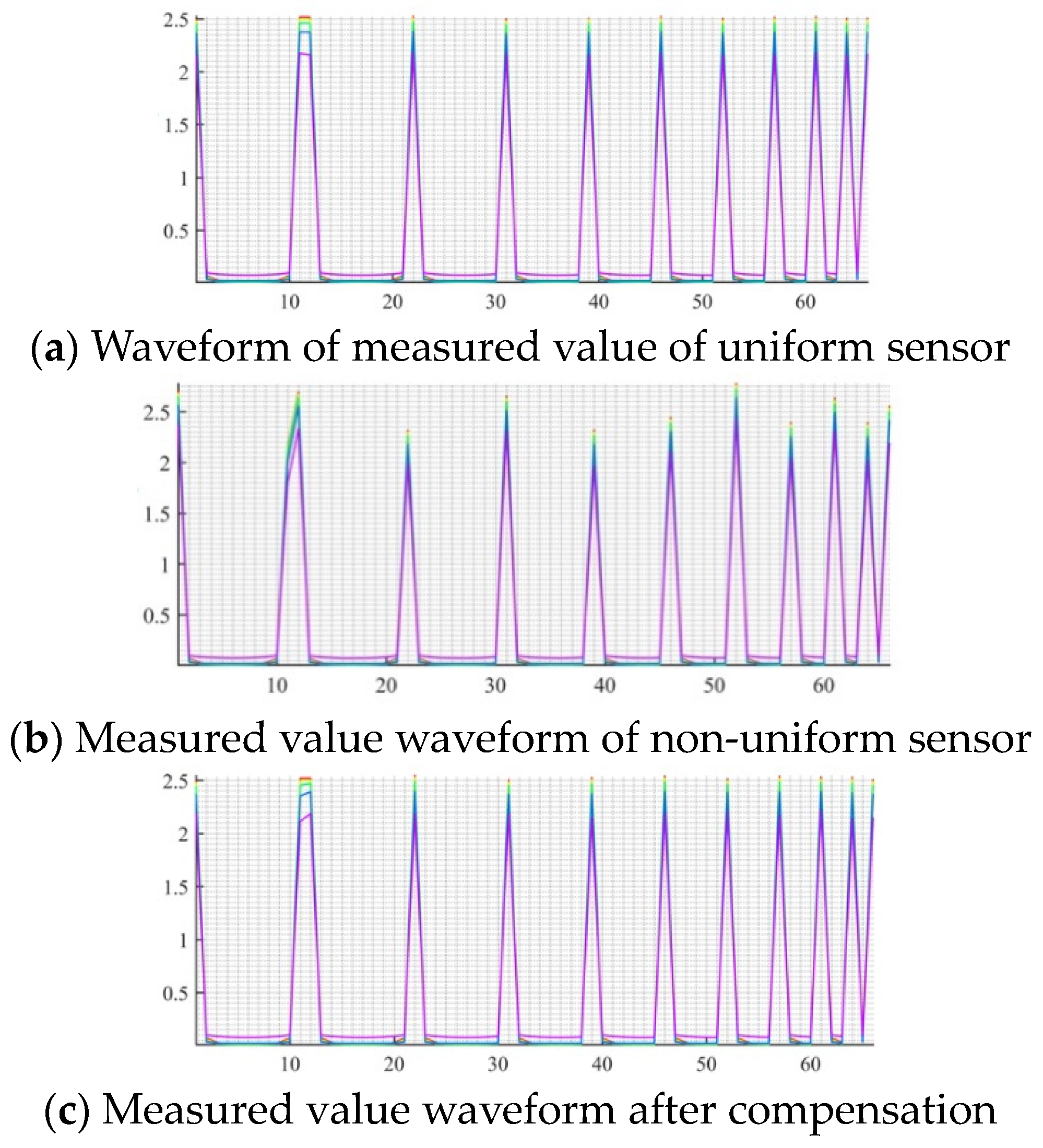
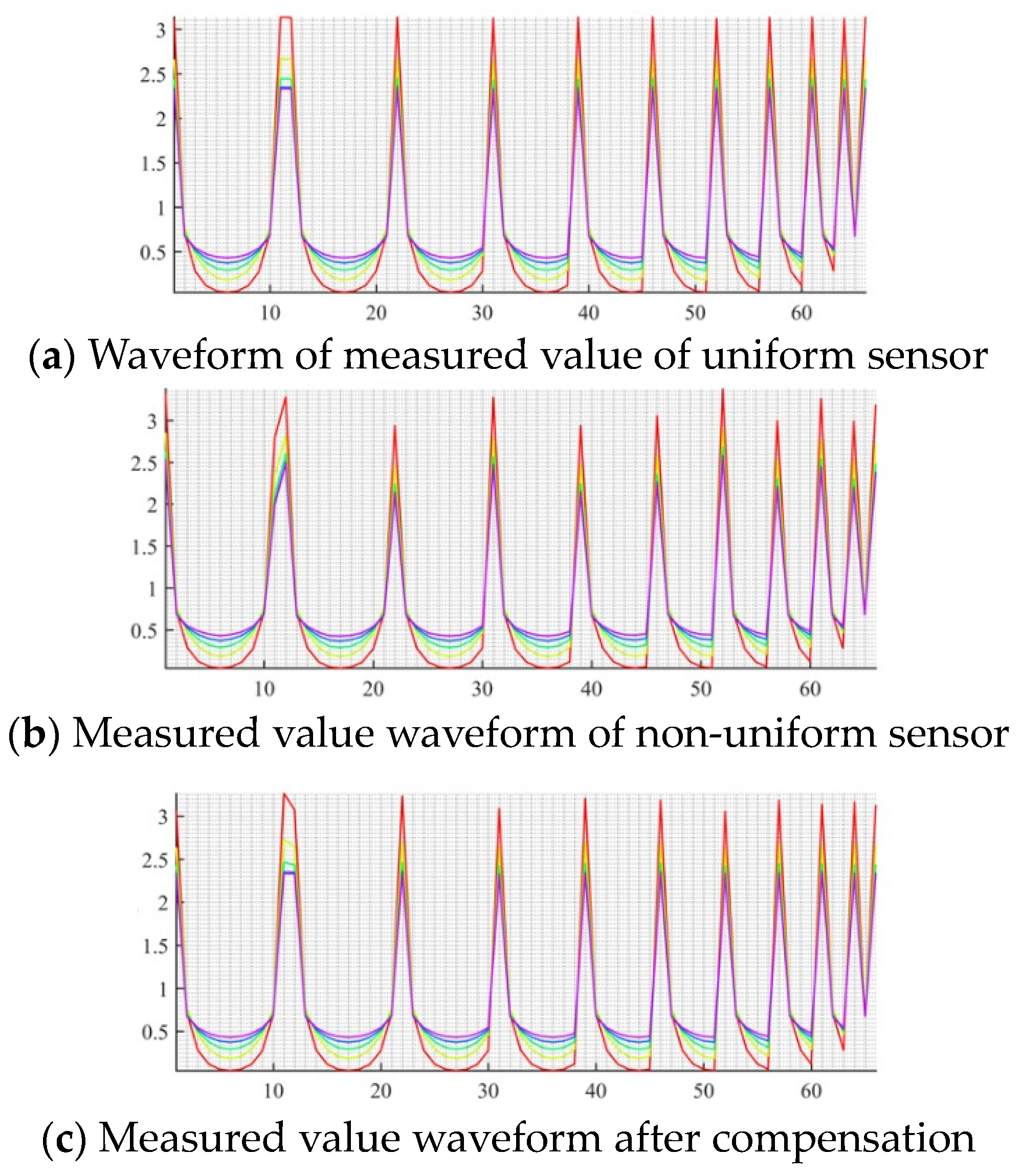
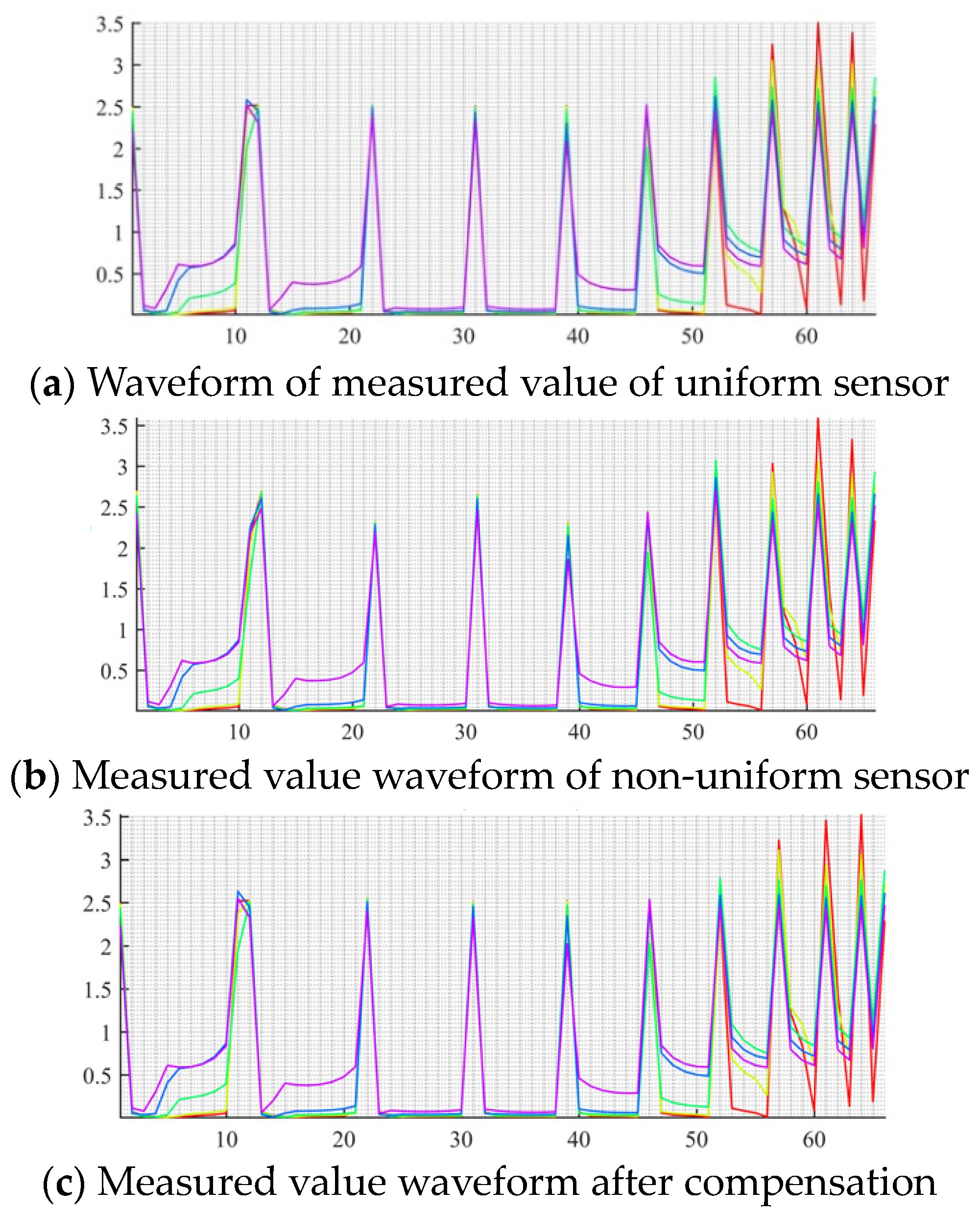
4. Simulation Experiment Verification

First, in COMSOL Multiphysics^®, the simulation model of 12-electrode ECT sensor is established. The simulation model parameters of sensing are set according to the actual sensors, and the parameters are listed in

Table 1. Parameter settings of fully uniform ECT sensor simulation model.

Parameter Description	Symbol	Numerical Value
Inside diameter of sensor pipe	Rp	25 mm
Sensor tube wall thickness	Dp	3 mm
Thickness of insulating filler layer	Di	10 mm
Relative dielectric constant of pipe wall	εp	3.7
Relative dielectric constant of insulating filler	εi	1
Sensor electrode length	Lp	125 mm
Sensor electrode coverage angle	α	26°
Electrode spacing angle	β	4°
Sensor excitation voltage	VE	1 V

. The schematic diagram of the finally established simulation model is shown in Figure 3.

Then, the simulation model of electrode spacing angle non-uniformity is established. When the simulation model of uneven spacing angle is established, the position of electrode 1 in Figure 3a remains unchanged, but the spacing angle between adjacent electrodes changes randomly: the change amount is [−0.2β, 0.2β] (i.e., [−0.8°, 0.8°]). Starting from electrode 1, the spacing angle between electrode i and its subsequent electrode is recorded as β_i.

Table 2. Electrode spacing angle parameter of heterogeneous ECT sensor.

Spacing Angle	Numerical Value	Spacing Angle	Numerical Value	Spacing Angle	Numerical Value
β1	4.0999°	β5	3.7165°	β9	4.1944°
β2	4.1515°	β6	4.3528°	β10	3.8251°
β3	3.6833°	β7	3.9397°	β11	3.9477°
β4	3.9912°	β8	3.9815°	β12	3.9799°

lists the sensor model with uneven electrode spacing angle β_i value. For sensors with uniform and non-uniform electrode spacing, except for the difference in spacing angle, the other parameter settings are completely the same.

In the above two sensor models, three media distributions, namely central flow, annular flow and laminar flow, are respectively set, as shown in Figure 4. During the simulation, laminar flow, central flow and annular flow are, respectively, set for the homogeneous and non-homogeneous sensors, and 5 phase holdups are taken as samples for each medium. The geometric parameters of medium distribution used for simulation are shown in

Table 3. Setting parameters of non-uniform ECT sensor simulation object field.

Medium Distribution	Control Parameters	Parameter Description	Value/mm
Central flow	Rw	Water column radius	2.5, 7.5, 12.5, 17.5, 22.5
Annular flow	Tw	Water ring thickness	2.5, 7.5, 12.5, 17.5, 22.5
Laminar flow	Hw	Water layer height	9, 17, 25, 33, 41

.

Figure 5 shows the waveforms of the measured values of a sensor with a completely uniform electrode spacing angle, a non-uniform sensor and a non-uniform sensor after compensation when the medium distribution is set to the center flow.

Figure 6 shows the waveforms of the measured values after compensation of the sensor with completely uniform electrode spacing angle, the sensor with non-uniform electrode spacing angle and the sensor with non-uniform electrode spacing angle when the medium distribution is set to the annular flow.

Figure 7 shows the waveforms of the measured values after compensation of the sensor with completely uniform electrode spacing angle, the sensor with non-uniform electrode spacing angle and the sensor with non-uniform electrode spacing angle when the medium distribution is set to laminar flow.

Note that the last three peak points in Figure 5, Figure 6 and Figure 7 correspond to the measured values of the three excitation detection pairs formed by adjacent electrodes. Therefore, theoretically, for symmetric flow patterns (annular flow and central flow), the three capacitance values should be completely equal. It can be seen that the law of the measured value of the sensor after compensation is more consistent with the law in theory, which indicates that the difference between the sensor waveform and the ideal sensor waveform is reduced after the compensation of the measured value.

The relative mean square error is calculated for the waveforms before and after compensation in Figure 5, Figure 6 and Figure 7 and the waveforms of the uniformity sensor, and the results are presented in

Table 4. The relative mean square error between the measured value of the non-uniform sensor before and after compensation and the measured value of the fully uniform sensor.

Sample No.	Central Flow RMSE/%		Annular Flow RMSE/%		Laminar Flow RMSE/%
	Before Compensation	After Compensation	Before Compensation	After Compensation	Before Compensation	After Compensation
1	7.51	0.56	5.75	1.96	7.05	1.81
2	7.56	0.54	6.83	0.97	6.80	1.47
3	7.69	0.52	6.86	0.34	6.73	1.32
4	7.98	0.57	7.05	0.05	6.64	1.01
5	8.73	1.34	7.04	0.04	7.05	1.16

. The calculation method of relative mean square error is as follows:

$$RMSE=\frac{{‖C-C^{*}‖}_2}{{‖C^{*}‖}_2}\times 100\%$$

(15)

where: $C$—capacitance measurement value vector of non-uniform sensor; $C^{*}$—measurement value vector of completely uniform sensor corresponding to $C$.

It can be seen from Table 4 that, before the measurement value compensation, the relative error between the measured value and the ideal value of the non-uniform sensor for the central flow, annular flow and laminar flow samples reaches 8.73%, 7.05% and 7.05%, respectively (samples 1 and 5). After compensation, the above relative errors are suppressed to 1.34%, 0.05% and 1.81% (sample 1)/1.16% (sample 5), respectively. After the compensation of the measured value, the relative error between the measured value and the ideal value of the non-uniform sensor is less than 2%, and the minimum is 0.04% (annular flow sample 5). Therefore, the measured value compensation has a good inhibition effect on the influence of sensor heterogeneity. The data in Table 4 prove the effectiveness of the measured value compensation method proposed in this paper.

5. Conclusions

In view of the measurement deviation of the ECT sensor caused by manufacturing and other reasons, the measurement value compensation method of the ECT sensor based on the assumption of invariable geometric factors proposed in this paper solves the problem of actual measurement error. The experiment proves that the SVM flow pattern classifier trained by the simulation data can effectively recognize the flow pattern of the measured data after the compensation of the measured value. Among the three flow patterns, the recognition rate of the annular flow and the central flow is as high as 100%, and the recognition rate of the laminar flow is as high as 93.75%. This provides a feasible solution for the accurate measurement of the multiphase flow pattern in the industrial field, and also opens a broad space for the application of ECT sensors in the field of mechanical equipment. At the same time, the relationship between the manufacturing accuracy of the ECT sensor and its measurement accuracy, ECT sensor materials and so on will become the research focus in the future.

Sensors analysis of different parameters involving two-phase flow can be constructed into volumetric analysis modelling [32]. Furthermore, in future implementation, one may use extreme learning algorithms [33,34] to identify interesting flow structures based on the sensing technique. The measurement of flow using sensors may be improved based on research using computational fluid dynamics simulation [35,36,37]. In particular, advancement in flexible operative instruments may be necessary as sensing of the flow parameters may have limitations.

References

1. Chen, F. External analysis of energy and environment problems. Acad. Forum 2013, 36, 146–151. [Google Scholar]
2. Tan, C.; Dong, F. Review of multiphase flow process parameter detection technology. Acta Autom. Sin. 2013, 39, 1923–1932. [Google Scholar] [CrossRef]
3. Fuchs, A.; Zangl, H.; Wypych, P. Signal modelling and algorithms for parameter estimation in pneumatic conveying. Powder Technol. 2007, 173, 126–139. [Google Scholar] [CrossRef]
4. Ismail, I.; Shafquet, A.; Karsiti, M.N. Application of electrical capacitance tomography and differential pressure measurement in an air-water bubble column for online analysis of void fraction. In Proceedings of the 2011 Fourth International Conference on Modeling, Simulation and Applied Optimization, Kuala Lumpur, Malaysia, 19–21 April 2011; pp. 1–6. [Google Scholar]
5. Niu, G.; Jia, Z.; Wang, J. Void Fraction Measurement in Oil-Gas Transportation Pipeline Using an Improved Electrical Capacitance Tomography System. Chin. J. Chem. Eng. 2004, 12, 476–481. [Google Scholar]
6. Shafquet, A.; Ismail, I. Measurement of void fraction by using electrical capacitance sensor and differential pressure in air-water bubble flow. In Proceedings of the 2012 4th International Conference on Intelligent and Advanced Systems (ICIAS2012), Kuala Lumpur, Malaysia, 12–14 June 2012; pp. 576–581. [Google Scholar]
7. Beck, M.S. Correlation in instruments-Cross correlation flowmeters. J. Phys. E Sci. Instrum. 2000, 14, 7–19. [Google Scholar] [CrossRef]
8. Ye, J.; Yang, W. Evaluation of Electrical Capacitance Tomography Sensors for Concentric Annulus. Sens. J. IEEE 2013, 13, 446–456. [Google Scholar] [CrossRef]
9. Yang, W. Design of electrical capacitance tomography sensors. Meas. Sci. Technol. 2010, 21, 447–453. [Google Scholar] [CrossRef]
10. Yang, W. Key issues in designing capacitance tomography sensors. In Proceedings of the Sensors, 2006, Daegu, Korea, 22–25 October 2006; IEEE: Piscataway, NJ, USA. [Google Scholar]
11. Zhang, L.; Wang, H.X. An iterative thresholding algorithm for the inverse problem of electrical resistance tomography. Flow Meas. Instrum. 2013, 33, 244–250. [Google Scholar] [CrossRef]
12. Cao, Z.; Wan, H.X. Optimization design of solid concentration capacitive sensor for gas-solid two-phase flow. Chin. J. Sci. Instrum. 2007, 28, 1956–1959. [Google Scholar]
13. Guo, S.; Li, X.; He, W. Gas and Solid Two Phase Flow Multi-parameter Measuring System Based on Capacitance Sensors of Double Array. Instrum. Tech. Sensor 2018, 4, 95–97. [Google Scholar]
14. Wang, H.G.; Yang, W.Q. Measurement of fluidised bed dryer by different frequency and different normalisation methods with electrical capacitance tomography. Powder Technol. 2010, 199, 60–69. [Google Scholar] [CrossRef]
15. Wang, H.X. Electrical Tomography; Science Press: Beijing, China, 2013. [Google Scholar]
16. Liu, S.; Lei, J.; Wang, X.Y.; Liu, Q.B. Generalized multi-scale dynamic inversion algorithm for electrical capacitance tomography. Flow Meas. Instrum. 2013, 31, 35–46. [Google Scholar] [CrossRef]
17. Huang, Z.Y.; Zhao, Y.; Wang, B.L.; Li, H.Q. Two phase flow pattern visualization system for electrical capacitance tomography. Chin. J. Sci. Instrum. 2001, 22, 458–461. [Google Scholar]
18. Li, K.; Wang, B.; Huang, Z.; Ji, H.; Li, H. Application of K-means clustering in flow pattern identification of CCERT system. J. Beijing Univ. Aeronaut. Astronaut. 2017, 043, 2280–2285. [Google Scholar]
19. Zhang, J.; Hu, H.; Dong, J.; Yan, Y. Concentration measurement of biomass/coal/air three-phase flow by integrating electrostatic and capacitive sensors. Flow Meas. Instrum. 2012, 24, 43–49. [Google Scholar] [CrossRef]
20. Wang, X.; Hu, H.; Zhang, A. Concentration measurement of three-phase flow based on multi-sensor data fusion using adaptive fuzzy inference system. Flow Meas. Instrum. 2014, 39, 1–8. [Google Scholar] [CrossRef]
21. Wang, X.; Hu, H.; Liu, X. Multisensor Data Fusion Techniques With ELM for Pulverized-Fuel Flow Concentration Measurement in Cofired Power Plant. IEEE Trans. Instrum. Meas. 2015, 64, 2769–2780. [Google Scholar] [CrossRef]
22. Thorn, R.; Johansen, G.A.; Hjertaker, B.T. Three-phase flow measurement in the petroleum industry. Meas. Sci. Technol. 2012, 24, 012003. [Google Scholar] [CrossRef]
23. Luo, Q.; Zhao, Y.F.; Ye, M.; Liu, Z.M. Application of electrical capacitance tomography in gas-solid fluidized bed measurement. CIESC J. 2014, 65, 2504–2512. [Google Scholar]
24. Wang, H.; Yang, W. Scale-up of an electrical capacitance tomography sensor for imaging pharmaceutical fluidized beds and validation by computational fluid dynamics. Meas. Sci. Technol. 2011, 22, 104015. [Google Scholar] [CrossRef]
25. Zhang, W.; Cheng, Y.; Wang, C.; Yang, W.; Wang, C.-H. Investigation on hydrodynamics of triple-bed combined circulating fluidized bed using electrostatic sensor and electrical capacitance tomography. Ind. Eng. Chem. Res. 2013, 52, 11198–11207. [Google Scholar] [CrossRef]
26. Guo, Q.; Meng, S.; Wang, D.; Zhao, Y.; Ye, M.; Yang, W.; Liu, Z. Investigation of gas–solid bubbling fluidized beds using ECT with a modified Tikhonov regularization technique. AIChE J. 2018, 64, 29–41. [Google Scholar] [CrossRef]
27. Che, H.; Wu, M.; Ye, J.; Yang, W.; Wang, H. Monitoring a lab-scale wurster type fluidized bed process by electrical capacitance tomography. Flow Meas. Instrum. 2018, 62, 223–234. [Google Scholar] [CrossRef]
28. Huang, K.; Meng, S.; Guo, Q.; Ye, M.; Shen, J.; Zhang, T.; Yang, W.; Liu, Z. High-temperature electrical capacitance tomography for gas–solid fluidised beds. Meas. Sci. Technol. 2018, 29, 104002. [Google Scholar] [CrossRef]
29. Li, X.; Jaworski, A.J.; Mao, X. Bubble size and bubble rise velocity estimation by means of electrical capacitance tomography within gas-solids fluidized beds. Measurement 2018, 117, 226–240. [Google Scholar] [CrossRef]
30. Zhu, X.; Dong, P.; Tu, Q.; Zhu, Z.; Yang, W.; Wang, H. Investigation of gas–solid flow characteristics in the cyclone dipleg of a pressurised circulating fluidised bed by ECT measurement and CPFD simulation. Meas. Sci. Technol. 2019, 30, 054002. [Google Scholar] [CrossRef]
31. Zeeshan, Z.; Zuccarelli, C.E.; Acero, D.O.; Marashdeh, Q.M.; Teixeira, F.L. Enhancing Resolution of Electrical Capacitive Sensors for Multiphase Flows by Fine-Stepped Electronic Scanning of Synthetic Electrodes. IEEE Trans. Instrum. Meas. 2019, 68, 462–473. [Google Scholar] [CrossRef]
32. Zhao, C.; Lv, J.; Du, S. Geometrical Deviation Modeling and Monitoring of 3D Surface Based on Multi-output Gaussian Process. Measurement 2022, 199, 111569. [Google Scholar] [CrossRef]
33. Tang, Z.; Wang, S.; Chai, X.; Cao, S.; Ouyang, T.; Li, Y. Auto-encoder-extreme learning machine model for boiler NOx emission concentration prediction. Energy 2022, 256, 124552. [Google Scholar] [CrossRef]
34. Lu, Y.; Fu, X.; Chen, F.; Wong, K.K.L. Prediction of fetal weight at varying gestational age in the absence of ultrasound examination using ensemble learning. Artif. Intell. Med. 2020, 102, 101748. [Google Scholar] [CrossRef]
35. Qian, M.; Niu, L.; Wong, K.K.L.; Abbott, D.; Zhou, Q.; Zheng, H. Pulsatile Flow Characterization in A Vessel Phantom With Elastic Wall Using Ultrasonic Particle Image Velocimetry Technique: The Impact of Vessel Stiffness on Flow Dynamics. IEEE Trans. Biomed. Eng. 2014, 99, 1–7. [Google Scholar] [CrossRef] [PubMed]
36. Wong, K.K.L.; Thavornpattanapong, P.; Cheung, S.C.P.; Tu, J.Y. Numerical Stability of Partitioned Approach in Fluid-Structure Interaction for a Deformable Thin-walled Vessel. Comput. Math. Methods Med. 2013, 2013, 638519. [Google Scholar] [CrossRef] [PubMed]
37. Liu, G.; Wu, J.; Huang, W.; Wu, W.; Zhang, H.; Wong, K.K.L.; Ghista, D.N. Numerical Simulation of Flow in Curved Coronary Arteries with Progressive Amounts of Stenosis Using Fluid-Structure Interaction Modelling. J. Med. Imaging Health Inform. 2014, 4, 605–611. [Google Scholar] [CrossRef]
Figure 1. ECT sensor machined with FPC electrode process and cut PEEK pipe process.
Electronics 11 02957 g001
Figure 2. The main process of manufacturing ECT sensor by sputtering process.
Electronics 11 02957 g002
Figure 3. Schematic diagram of geometric parameters of sensor simulation model.
Electronics 11 02957 g003
Figure 4. Schematic diagram of simulation object field setting of heterogeneous ECT sensor.
Electronics 11 02957 g004
Figure 5. Waveforms of measured values before and after center current compensation.
Electronics 11 02957 g005
Figure 6. Waveforms of measured values before and after annular flow compensation.
Electronics 11 02957 g006
Figure 7. Waveforms of measured values before and after laminar flow compensation.
Electronics 11 02957 g007