Influence of the Stiffness of the Robotic Arm on the Position of the Effector of an EOD Robot

Abstract

Terrestrial robots are being employed in a variety of sectors and for a variety of objectives. The purpose of this paper is to analyze and validate an analytical–numerical model of a robotic arm’s behavior. The proposed robot was designed to replace human personnel who remove ammunition or explosive devices. At the same time, the influence of the stiffness of the EOD robotic arm on the position of the effector in a variety of geometric task configurations was investigated. In order to obtain results relevant to the investigation, the angles of rotation under the load of each component of the arm’s composition and the vertical movement of the effector were measured. The main conclusions emphasize that a lower stiffness comes from the components of linear motors, which act on the elements of the robotic arm, and they substantially influence the elastic behavior of the arm. In addition, the constructive components of the arm have high rigidity compared to those of the linear actuators.

1. Introduction

Robotic explosive ordnance disposal (EOD) systems can carry out reconnaissance, detection, disposal, and transport missions of explosives. As can be seen in [1,2,3,4], intervention robots for artisanal pyrotechnic devices are influenced by the accuracy of the effector mechanism. Additionally, their use in teleoperated mode implies that the information from the sensors ensures a prediction of the final actuation position [2]. There are constructive solutions for EOD robots equipped with a multitude of drive systems (excavator buckets and manipulator arms [3] are very useful, especially for work area cleaning activities), but the fact that they have too many drive systems may lead to the introduction of additional positioning errors. The simultaneous operation of this equipment or its positioning causes oscillations in the position of the robot’s center of gravity. Therefore, we consider that, depending on the EOD-type missions, a robot must be built to perform only certain missions [4]. Because of fundamental modifications in command and control algorithms, EOD robots can also become intervention robots in high-risk situations [5].

Structural changes allow intervention crews such as firefighters and anti-terror units to intervene in disasters caused by fires [6,7]. From [8], it can be seen that the use of EOD robots has become a priority for the protection of intervention personnel, especially in the case of anti-personnel mines. Another aspect pursued in the realization of robots is the simultaneous operation of the propulsion system and the actuation system, in order to reduce intervention times, without compromising the accuracy of the final effector [9,10]. From a structural point of view, EOD robots are systems that consist of:

• Sensors for environmental perception [11,12,13]: in addition to sensors for obstacle detection, image sampling, and environmental conditions, simple sensors, such as potentiometers, limit switches (especially for limiting the travel of robotic arm elements), telemetry and current sensors, and temperature sensors for monitoring electronic equipment, are also required on the robot.
• Execution elements for performing actions on the environment [14,15,16,17,18,19], which are composed of linear, rotary, electric, hydraulic, or pneumatic motors; effector mechanisms have different configurations of the gripping mechanism, so that they can safely grasp the various objects, or even be able to operate “manually” on handcrafted devices. The choice and assembly of the execution elements on the robot chassis must be simple enough to reduce the preparation time of the intervention, and last but not least, the choice of engine types (transmission, robotic arm) should be made taking into account at least two parameters—current consumption and the load to be lifted/moved.
• Propulsion systems, which ensure the movement to the target and back and can even perform rotations/elevations to supplement the shoulder of the degrees of freedom of the robot; these propulsion systems may be on wheels, tracks, or mixed. Regardless of the propellant solution chosen, performing the turn involves friction with the ground, so for the present study, we considered that the most suitable is the crawler propulsion system [20,21,22,23]. From the analysis of the references, there is another important conclusion related to the stability in operation of the robot depending on the specific pressure on the ground. In the case of using a wheeled propulsion system, the sinking increases when the robotic arm lifts objects, at the position of the center of gravity, meaning that the robot controller must make additional corrections as regards the repositioning of the final effector.

It is important to mention that EOD robots intended for intervention in the disposal and transport of explosives must not be excessively equipped with sensors as there is a risk of damage during the execution of those missions [24,25].

Depending on how they are organized on the robot chassis, they can help to create a semi-autonomous/autonomous navigation system. This is very important because the missions in which EOD robots will be involved can endanger the lives of human operators. Therefore, a sensor system that allows the use of robots in optimal conditions will have to contain the following sensors (not always in this configuration): LIDAR, GPS [26,27,28,29], proximity (ultrasonic, IR), video cameras (monoculation/stereo), radar, displacement, force sensor [30], inertial navigation system [31]. From the analysis of the very wide spectrum of sensors that can be part of an EOD robot, it results that their value can exceed that of the chassis and the robotic arm [32,33,34,35]. The advantages of using low-cost EOD robot solutions lie mainly in the fact that they can be destroyed during missions. Additionally, the use of relatively inexpensive hardware components guarantees a fast interconnection and does not involve a complex and expensive infrastructure. The use of commercial components allows the creation of families of EOD robots that work as a family, and the communication system can be developed around XBee platforms.

As can be seen, we are dealing with a multitude of situations, which highlight two things: the complexity of robotic EOD systems and the ability to intervene at low cost, as these robots can be destroyed during missions. That is why we consider it opportune to study how the rigidity of the robotic arm can influence the actuation accuracy of the final effector.

The focus of this paper was to investigate and evaluate the validity of an analytical–numerical model that was developed to describe how a robotic arm performs. The authors set this goal because, in the literature, no references can be identified regarding the evaluation of the positioning accuracy of the effector arm. The EOD robot proposed is a teleoperated one, meaning that the navigation is performed by the operator, and the crawler propeller is suitable for indoor/outdoor missions.

Meanwhile, this robot with elasticity in the arm is of the middle class, being able to operate in different environments (unstructured) both indoors and outdoors. This indoor/outdoor operating capability is mainly due to the fact that it is a teleoperated robot. Another factor that contributes to the increase in the operating capacity is the fact that the propeller is a crawler thruster, having very good capacity for progression in the field. It should be noted that the structure of the crawler propeller allows the robot to climb obstacles and stairs.

The factors that led to the current study are as follows:

• Conditions imposed by the type of crawler thruster or the existing track type [36,37,38]: The fact is that the use of tracked vehicles leads to a specific pressure on the ground, which can, among other things, facilitate a much quieter movement, especially if the track is made of rubber; another good element to take into account is the analytical model that describes the turning, meaning that we can obtain a prediction regarding the effects due to the resistance to turning (diving, slipping, skidding). We consider all of this to influence the actuation accuracy of the final effector.
• Limitations due to the level of uncertainty associated with the different artisanal pyrotechnic systems, which are usually unique, the reinforcement mechanisms, and the way they are made, differing from case to case [39,40,41]. The uncertainties that arise result from the analysis of data obtained by measuring various parameters: temperature, pressure, wind direction/air currents, the evolution of the flame front, the characteristics of the explosion, and the materials that can be caused by the blast. In relation to the reinforcement mechanisms, following the scanning of artisanal devices, it is not possible to obtain sufficient data to know how to orient the disruptor, which can even lead to triggering the respective device; in general, these devices are unique, with their designers trying to make them as complex as possible.
• Material characteristics specific to the structure of the robotic arm [42,43]: from this point of view, in order for the robot to be able to perform the tasks, and considering the fact that the shape of the arm must be configured to pass electrical cables, the motors, sensors, and frame must be made of rigid materials, which should be elastic but not easy to break due to loads with additional weights.

The formulation of the task from the point of view of our own research refers to:

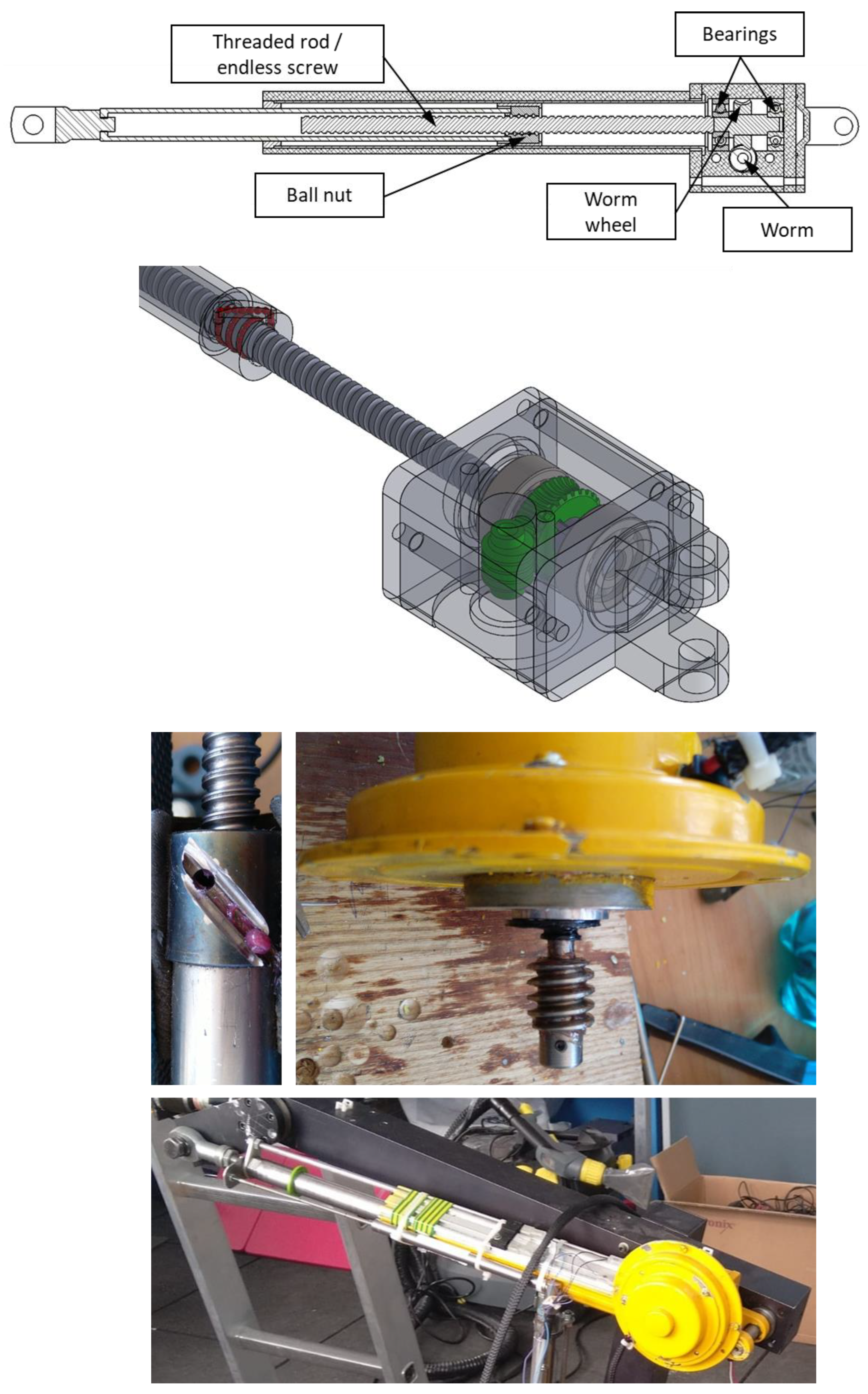
• The possibility of slipping in the ball mechanism of each component element; the guide system of the arm elements consists of a ball bearing encased in an endless nut/screw system.
• Establishing an analytical–numerical model for the calculation of direct and inverse kinematics [44].
• Testing and evaluation of the final effector positioning system for different geometric configurations of the robotic arm.

Because the intervention preparation is short, this EOD robot system provides an optimum solution in terms of operational and maintenance expenses. In contrast, the instability of the final effector positioning leads to relatively long operating times. Therefore, the present study aimed to highlight these instabilities, based on the study of the elasticity of the robotic arm. The robot must intervene in the removal of pyrotechnic devices without causing further damage, in order to replace human personnel.

The accuracy of the positioning of the effector considers:

-

The elasticity of the component elements;

-

Deviations and inertia from the drive system.

The working conditions of EOD robots are often difficult. Their intervention takes place in unstructured environments, full of obstacles and bumps. All these generate special maneuverability conditions, which in turn affect the operational stability of the final effector. The literature provides algorithms for kinematic and dynamic analysis of robotic arms in ideal conditions or for operation in structured environments. From the measurements performed on the arm in different operating configurations, we found that the return to the “0” position is the same. This led us to test each component of the arm separately, in order to obtain information about the manufacturing games and those that appeared as a result of the operation. Based on this information, we started to study the robotic arm from an analytical, numerical, and experimental point of view. We considered that the resulting analytical model will allow the introduction of a new algorithm in the robot controller, which would allow the smooth (not to be discontinuous) operation of the robotic arm.

This paper is organized into six sections. Section 2 describes the mechanism under analysis. Section 3 deals with the analytical–numerical models of the robotic arm. Section 4 presents the results of the analytical–numerical simulation using the finite element method, for the analytical determination of the arm behavior for different geometric configurations, and of the tasks of the gripper. Section 5 presents the synthesis of the analytical–numerical analysis and compares this with the data obtained experimentally. Section 6 presents the conclusions and the potential for further development of the proposed method to improve the positioning accuracy of the robotic arm, depending on the degree of elasticity of the components and the assembly when it is subjected to the direct action of different tasks in the regime, static and dynamic.

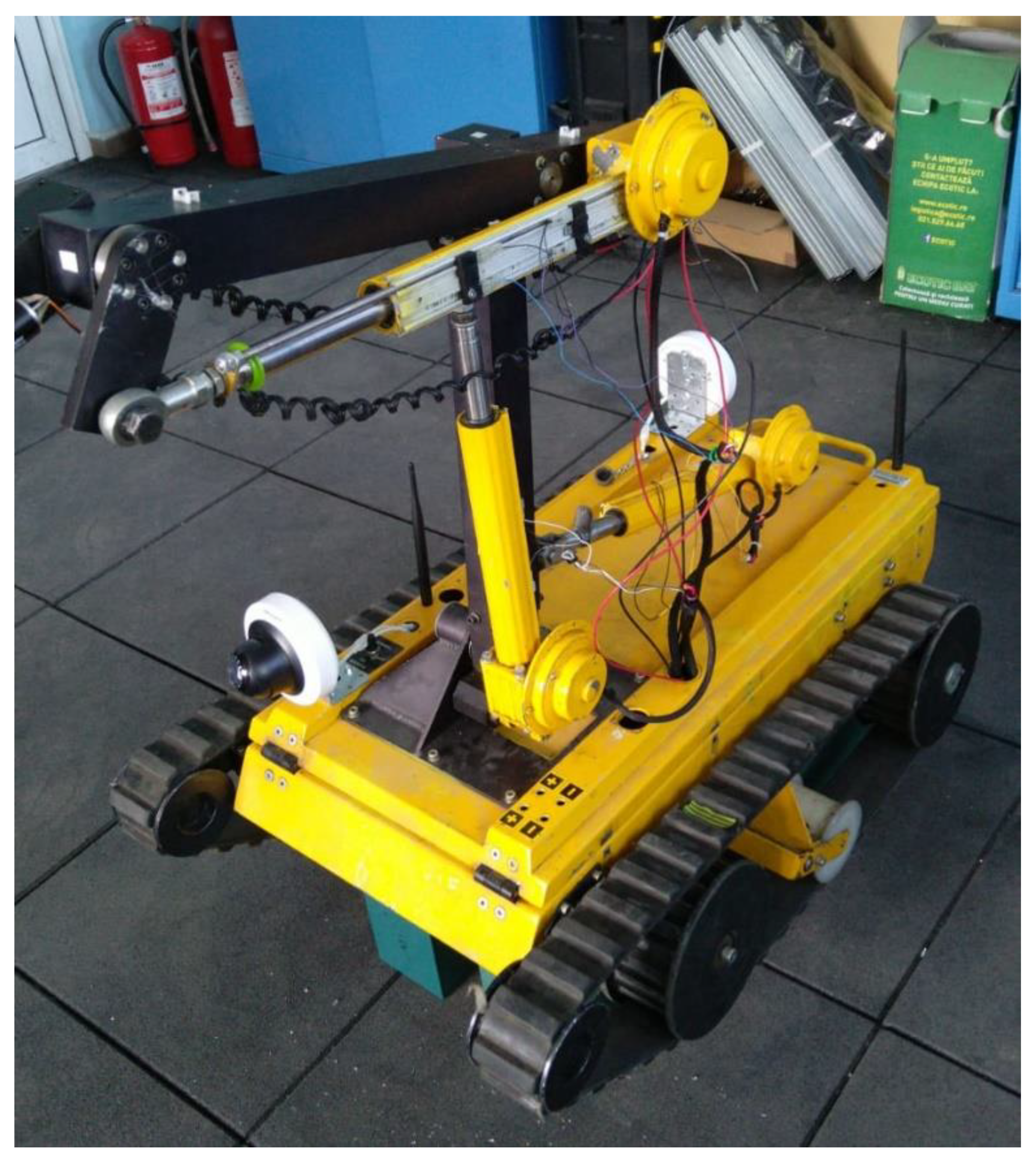
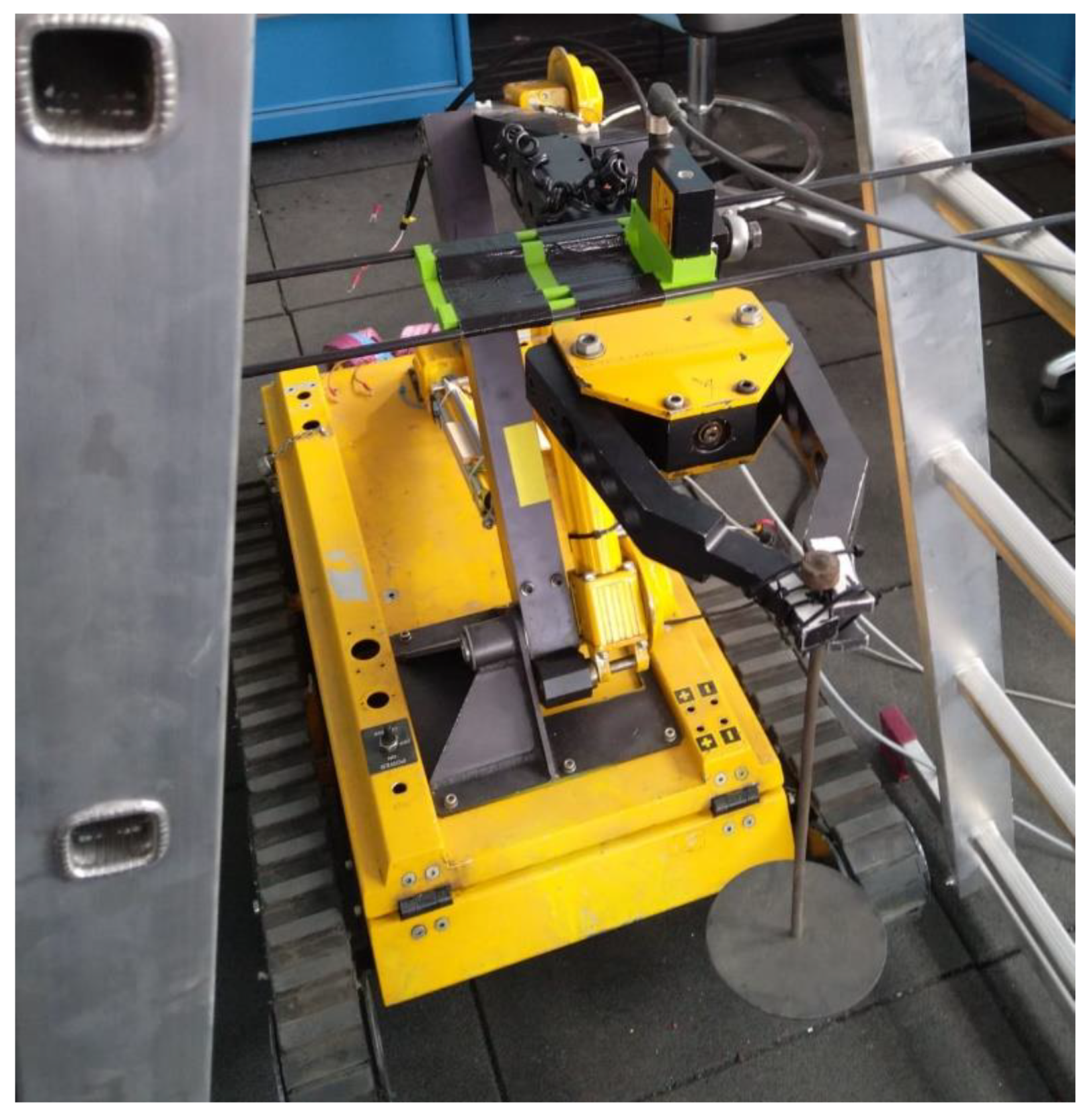
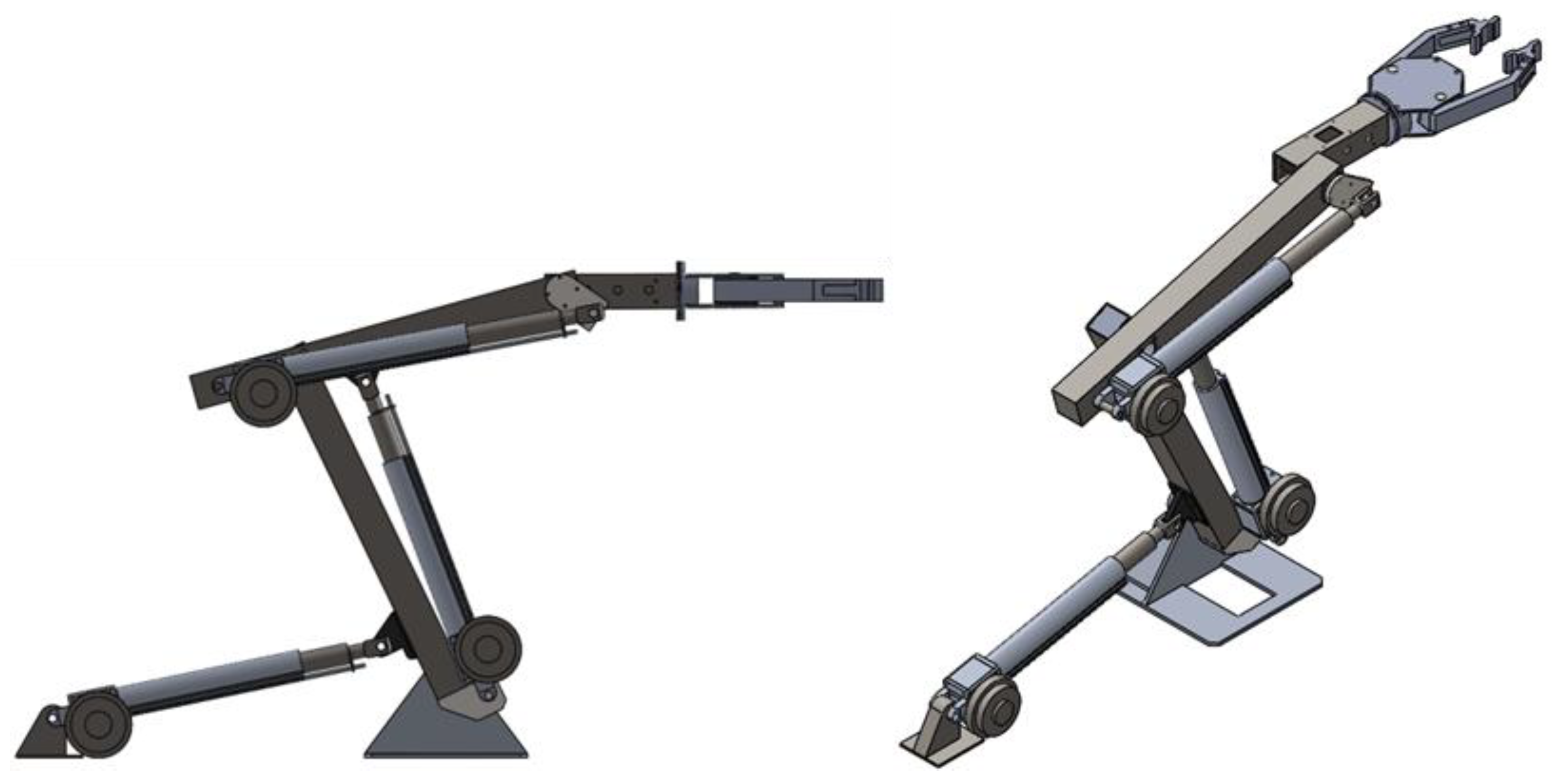
2. Mechanism Description—EOD Robot with Robotic Arm

The studied robot is an EOD robot used for monitoring and interventions of artisanal pyrotechnic devices (Figure 1).

From a functional point of view, the robot consists of a chassis, a crawler propulsion system, robotic arms, and an effector mechanism. To perform the tests, the composition of the robot also includes a hook on which the working weights of 0.555 kg, 1 kg, and 5 kg, or combinations thereof, will be weighed (Figure 2).

The configuration that we considered aims to highlight the vertical displacements of the effector. These displacements were analyzed for several cases, with different loads and different angles of rotation of the robotic arm drive motors.

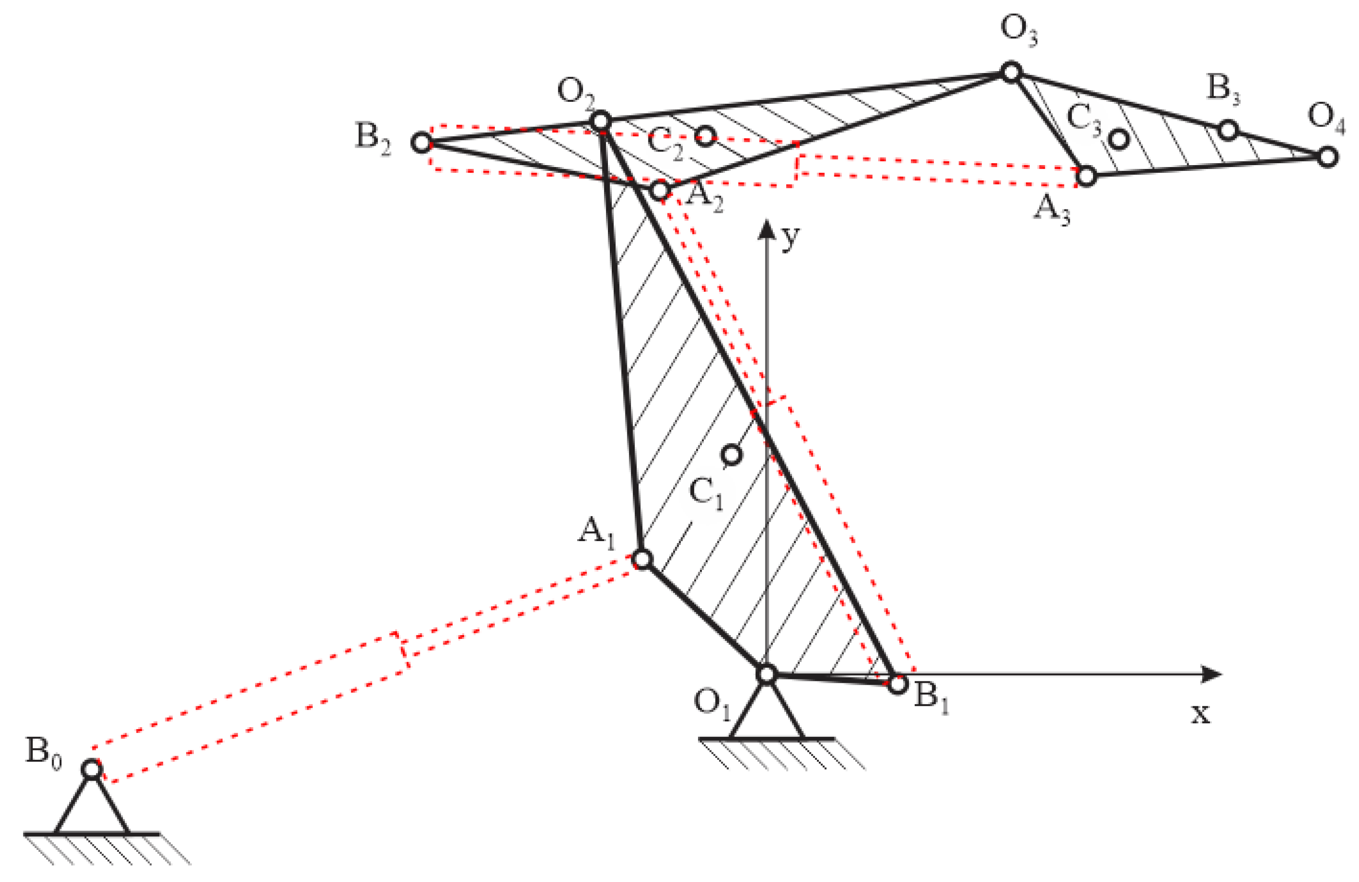
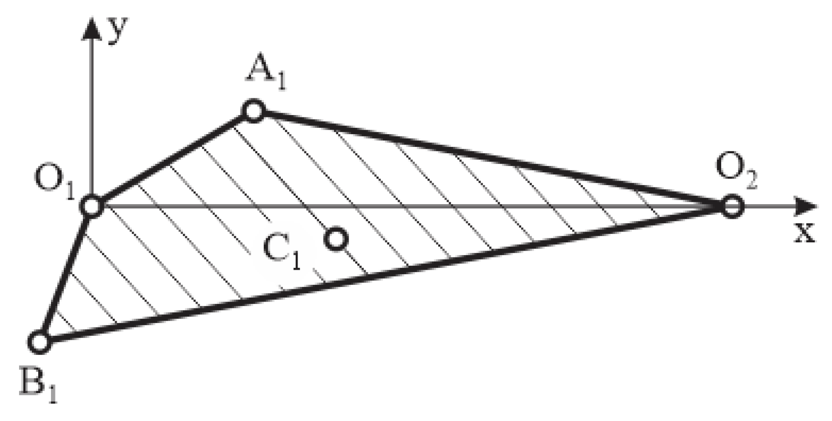
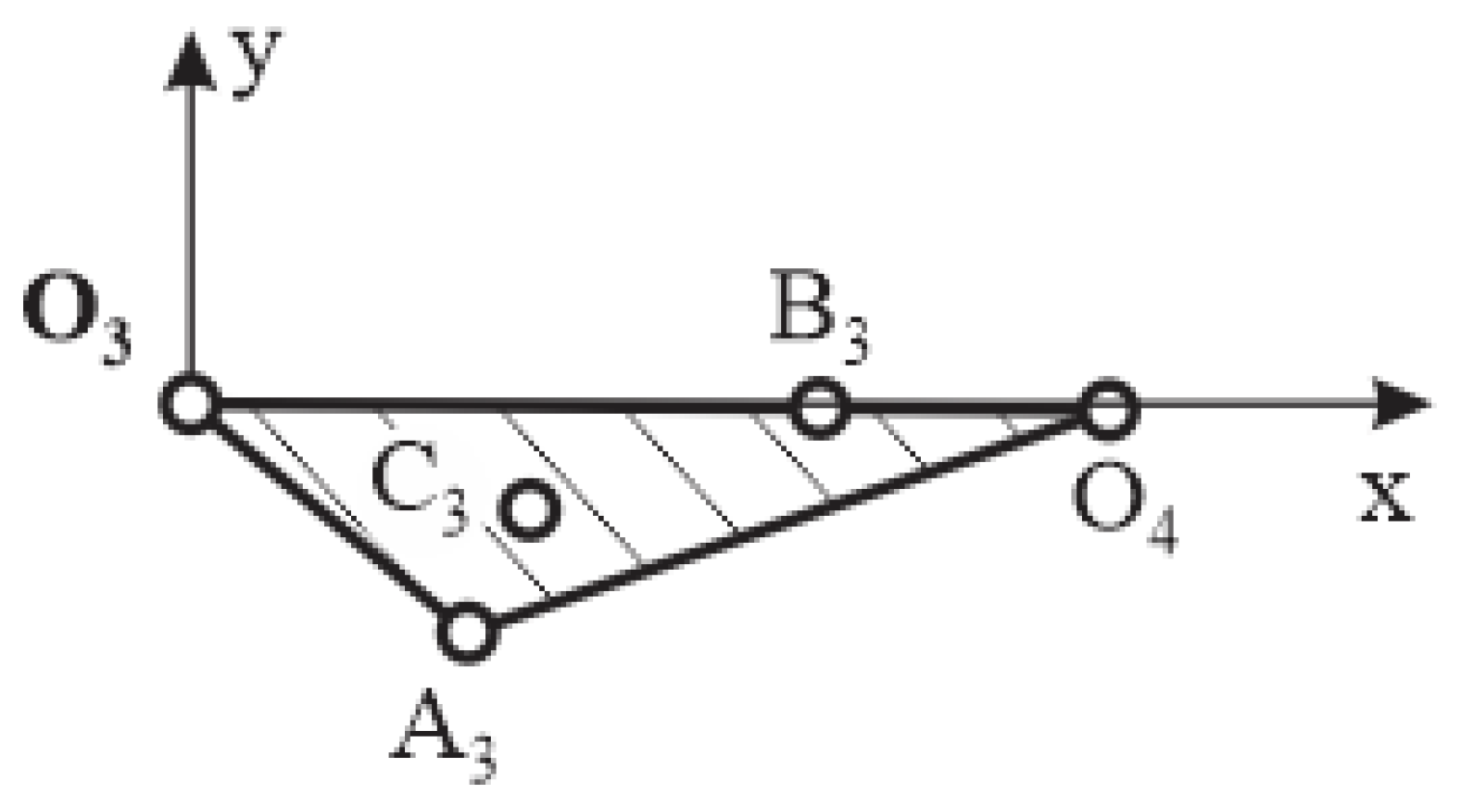
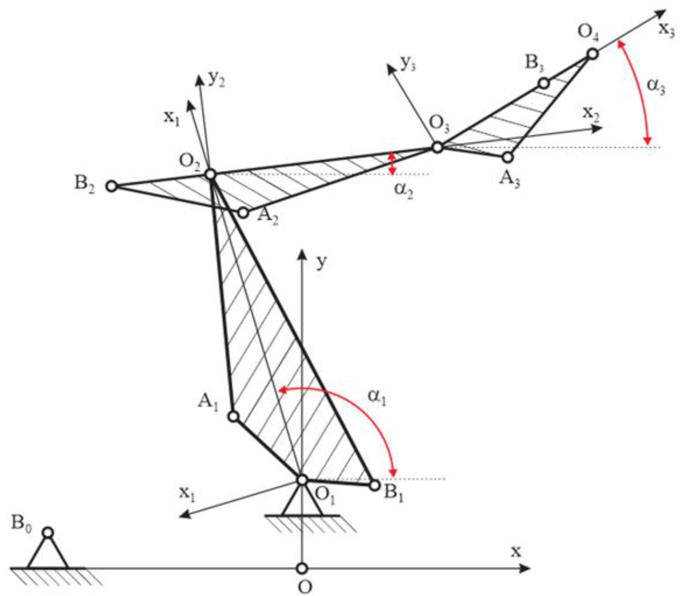
3. Geometric Description of the Working Configurations of the Robotic Arm

For the geometric representation in Figure 3, we have the following explanations: The articulation of arm 1 with the robot chassis is denoted by O₁, that between arms 1 and 2 is denoted by O₂, and that between arms 2 and 3 is denoted by O₃. The rest of the notations bear the index finger.

At point B₃, vertical displacement is measured using a laser displacement sensor. Figure 4, Figure 5 and Figure 6 show the robot’s arms separately with their local system.

Table 1. Coordinates of points of interest in relation to the local coordinate systems.

Arm No. 1			Arm No. 2			Arm No. 3
	x	y		x	y		x	y
O1	500	0	O2	400	0	O3	400	0
A1	80.94	65	A2	90.5	−51	A3	44.8	−31.4
B1	−50	−44	B2	−128	0	B3	300	−44
C1	230.12	−2.4	C2	165.5	−1.3	C3	230.12	−2.4

shows the coordinates of the centers of mass of the arms, the positions of the joints between the arms and between the arms and the linear motors, the point of application of the force, and the point where the displacement is measured.

The angular positions of the coordinate systems related to the arm components are measured with respect to the fixed coordinate system, the positive direction being the trigonometric one (Figure 7).

Below are five working configurations, which are presented in

Table 2. The angles of the three elements of the robotic arm, corresponding to the working configurations.

Working Configuration	Arm No. 1	Arm No. 2	Arm No. 3
Configuration 1	115.6	15.4	0.2
Configuration 2	104.7	15.7	0
Configuration 3	0.1	5.6	0.1
Configuration 4	74.8	5.8	0.4
Configuration 5	58.6	6.0	0.4

, each of which is characterized by the angles of the arms to the general reference system; as an example, a generic representation is presented in Figure 8.

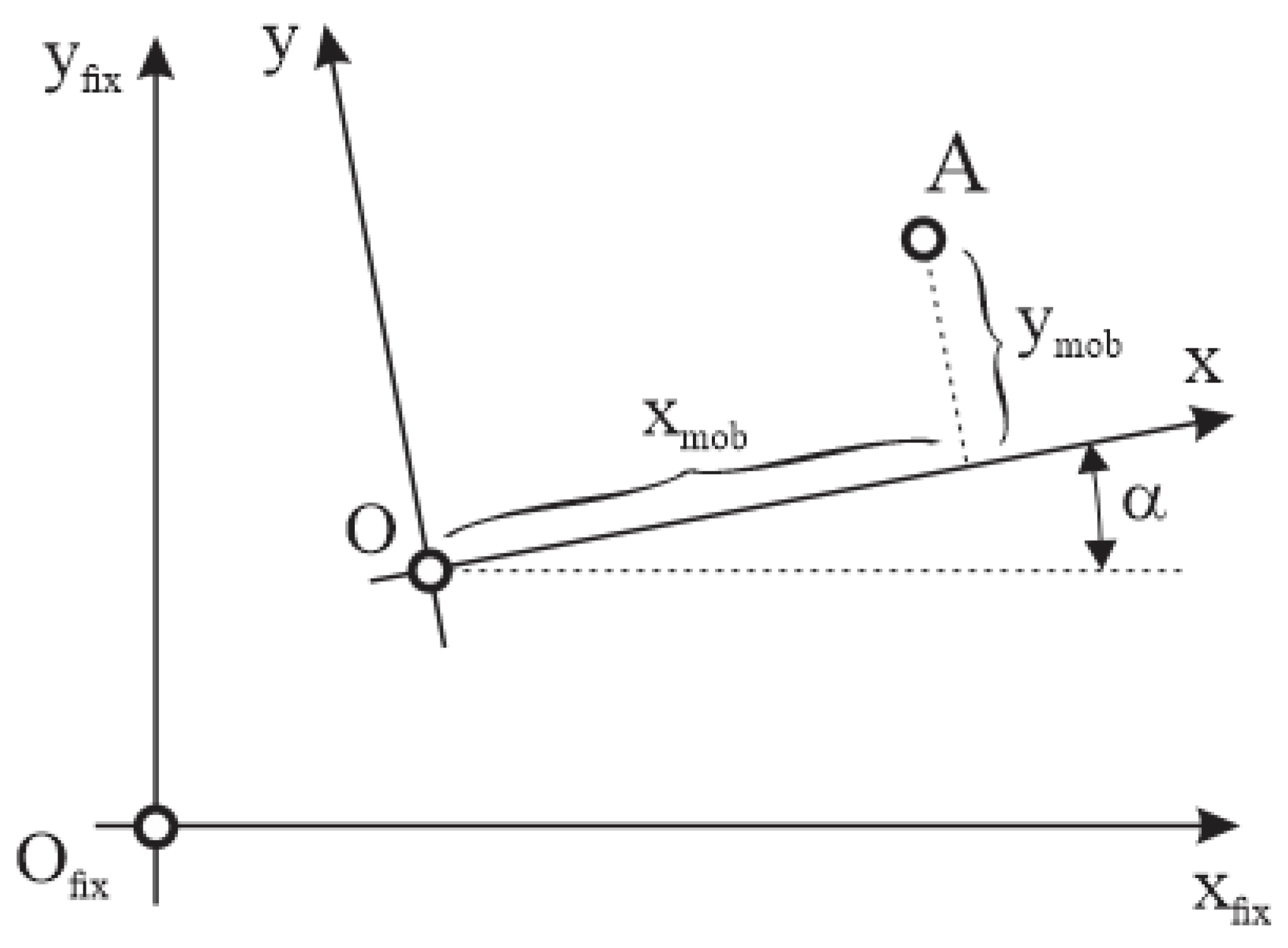
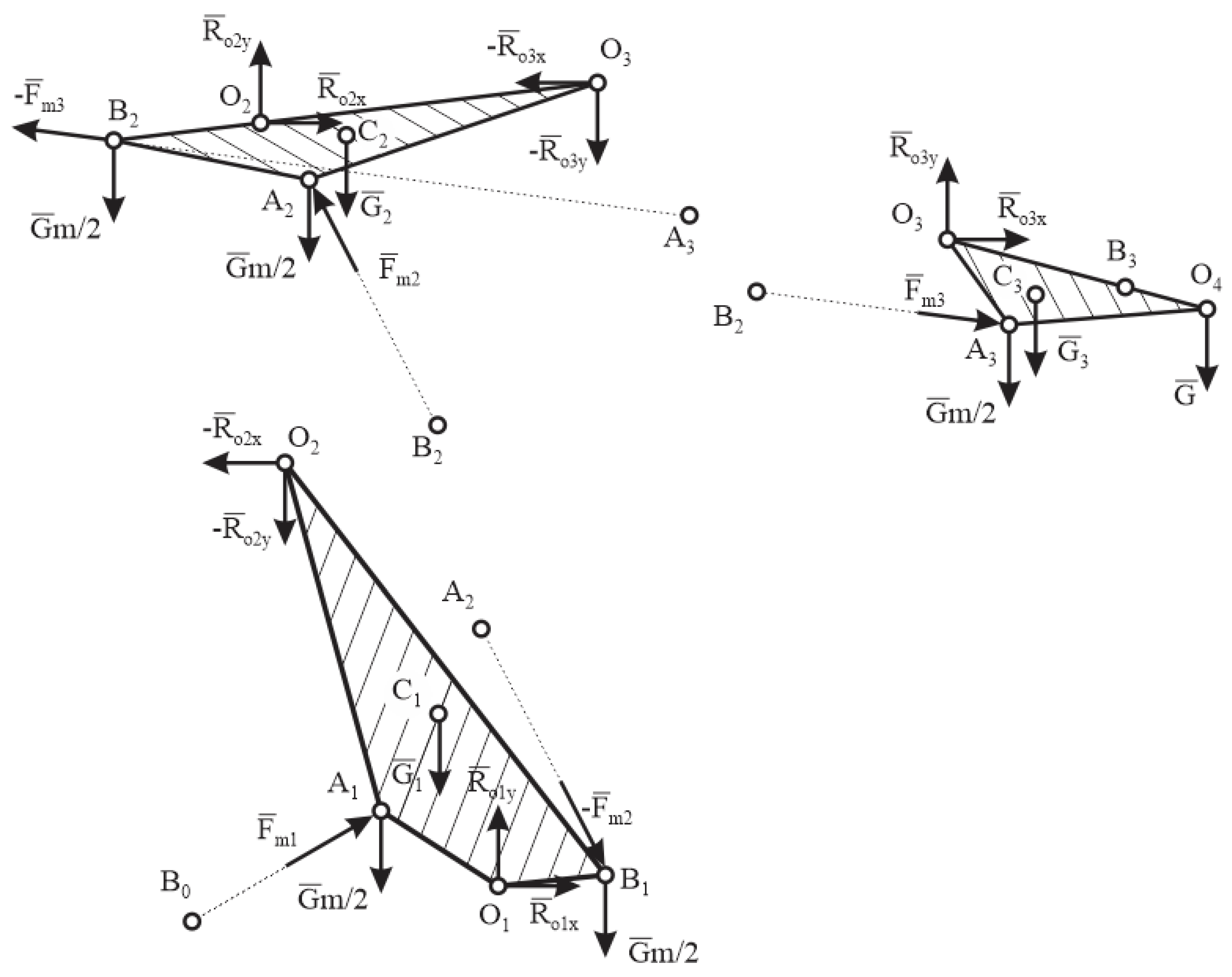
4. Analytical Modeling

For the analytical model, the arm is considered as a planar mechanism, with three degrees of freedom (Figure 9).

The relationship between the coordinates of a point relative to the fixed coordinate system and that of a robot arm (Figure 9) is

$$\{\begin{array}{c}{x}_{fix}=x_{\mathrm{O}}+x_{mob}\cdot \cos \alpha -y_{mob}\sin \alpha \\ y_{fix}=y_{\mathrm{O}}+x_{mob}\cdot \sin \alpha +y_{mob}\cos \alpha \end{array} ,$$

(1)

With the help of this relation, the coordinates of the points of interest with respect to the fixed coordinate system can be determined.

Assuming a rigid solid behavior of the robotic arm components, the connecting forces in the joints and the axial forces in the motors can be calculated for the five configurations (Figure 10).

For the situation where the weights of the motors are evenly distributed between the joints, the equilibrium equations for arm 3 and the effector are given by

$$\begin{gathered} \{\begin{array}{l}{\displaystyle \sum F_x}=0:R_{{\mathrm{O}}_{3}x}+F_{m3}\cdot n{23}_x=0\hfill \\ {\displaystyle \sum F_y}=0:R_{{\mathrm{O}}_{3}y}-\frac{Gm}{2}-G_3-G+F_{m3}\cdot n{23}_y=0\hfill \end{array} , \\ \begin{array}{ll}{\displaystyle \sum M_{{\mathrm{O}}_{3}z}}& =0:F_{m3}\cdot \left[n{23}_y\cdot \left(x_{{\mathrm{A}}_3}-x_{{\mathrm{O}}_3}\right)-n{23}_x\cdot \left(y_{{\mathrm{A}}_3}-y_{{\mathrm{O}}_3}\right)\right]\\ & -\frac{Gm}{2}\cdot \left(x_{{\mathrm{A}}_3}-x_{{\mathrm{O}}_3}\right)-G_3\cdot \left(x_{{\mathrm{C}}_3}-x_{{\mathrm{O}}_3}\right)-G\cdot \left(x_{{\mathrm{O}}_4}-x_{{\mathrm{O}}_3}\right)=0\end{array} \end{gathered}$$

(2)

where $\overrightarrow{n23}=\frac{\left(x_{{\mathrm{A}}_3}-x_{{\mathrm{B}}_2}\right)\cdot \overrightarrow{i}+\left(y_{{\mathrm{A}}_3}-y_{{\mathrm{B}}_2}\right)\cdot \overrightarrow{j}}{\sqrt{{\left(x_{{\mathrm{A}}_3}-x_{{\mathrm{B}}_2}\right)}^2+{\left(y_{{\mathrm{A}}_3}-y_{{\mathrm{B}}_2}\right)}^2}}$.

It follows from the equation of moments $F_{m3}$ and the values of the connecting force components in joint ${\mathrm{O}}_3$ that

$$\{\begin{array}{l}{F}_{m3}=\frac{\frac{Gm}{2}\cdot \left(x_{{\mathrm{A}}_3}-x_{{\mathrm{O}}_3}\right)+G_3\cdot \left(x_{{\mathrm{C}}_3}-x_{{\mathrm{O}}_3}\right)+G\left(x_{{\mathrm{O}}_4}-x_{{\mathrm{O}}_3}\right)}{n{23}_y\cdot \left(x_{{\mathrm{A}}_3}-x_{{\mathrm{O}}_3}\right)-n{23}_x\cdot \left(y_{{\mathrm{A}}_3}-y_{{\mathrm{O}}_3}\right)}\hfill \\ R_{{\mathrm{O}}_{3}x}=-F_{m3}\cdot n{23}_x\hfill \\ R_{{\mathrm{O}}_{3}y}=\frac{Gm}{2}+G_3+G-F_{m3}\cdot n{23}_y\hfill \end{array} ,$$

(3)

For arm 2, the static equilibrium equations are

$$\begin{gathered} {\displaystyle \sum F_x}=0:-R_{{\mathrm{O}}_{3}x}-F_{m3}\cdot n{23}_x+F_{m2}\cdot n{12}_x+R_{{\mathrm{O}}_{2}x}=0, \\ \begin{array}{ll}{\displaystyle \sum F_y}=0:& -R_{{\mathrm{O}}_{3}y}-F_{m3}\cdot n{23}_y+F_{m2}\cdot n{12}_y+R_{{\mathrm{O}}_{2}y}\\ & -\frac{Gm}{2}-\frac{Gm}{2}-G_2=0\end{array}, \\ \begin{array}{ll}{\displaystyle \sum M_{{\mathrm{O}}_{3}z}}& =0:F_{m3}\cdot \left[n{23}_y\cdot \left(x_{{\mathrm{B}}_2}-x_{{\mathrm{O}}_2}\right)-n{23}_x\cdot \left(y_{{\mathrm{B}}_2}-y_{{\mathrm{O}}_2}\right)\right]\\ & -\frac{Gm}{2}\cdot \left(x_{{\mathrm{A}}_2}-x_{{\mathrm{O}}_2}\right)-G_3\cdot \left(x_{{\mathrm{B}}_2}-x_{{\mathrm{O}}_2}\right)-G_2\cdot \left(x_{{\mathrm{C}}_2}-x_{{\mathrm{O}}_2}\right)\\ & +F_{m2}\cdot \left[n{21}_y\cdot \left(x_{{\mathrm{A}}_2}-x_{{\mathrm{O}}_2}\right)-n{12}_x\cdot \left(y_{{\mathrm{A}}_2}-y_{{\mathrm{O}}_2}\right)\right]\\ & +R_{{\mathrm{O}}_{3}x}\cdot \left(y_{{\mathrm{O}}_3}-y_{{\mathrm{O}}_2}\right)-R_{{\mathrm{O}}_{3}y}\cdot \left(x_{{\mathrm{O}}_3}-x_{{\mathrm{O}}_2}\right)=0\end{array} \end{gathered}$$

(4)

where $\overrightarrow{n12}=\frac{\left(x_{{\mathrm{A}}_2}-x_{{\mathrm{B}}_1}\right)\cdot \overrightarrow{i}+\left(y_{{\mathrm{A}}_2}-y_{{\mathrm{B}}_1}\right)\cdot \overrightarrow{j}}{\sqrt{{\left(x_{{\mathrm{A}}_2}-x_{{\mathrm{B}}_1}\right)}^2+{\left(y_{{\mathrm{A}}_2}-y_{{\mathrm{B}}_2}\right)}^2}}$.

The axial force in linear motor 2 results from the equilibrium equation at times

$$\begin{array}{l}{F}_{m2}=\frac{F{m}_3\left[n{23}_y\left(x_{{\mathrm{B}}_2}-x_{{\mathrm{O}}_2}\right)-n{23}_x\left(y_{{\mathrm{B}}_2}-y_{{\mathrm{O}}_2}\right)\right]}{n{12}_y\left(x_{{\mathrm{A}}_2}-x_{{\mathrm{O}}_2}\right)-n{12}_x\left(y_{{\mathrm{A}}_2}-y_{{\mathrm{O}}_2}\right)}\\ +\frac{\frac{Gm}{2}\left(x_{{\mathrm{B}}_2}-x_{{\mathrm{O}}_2}\right)+G_2\left(x_{{\mathrm{C}}_2}-x_{{\mathrm{O}}_2}\right)+\frac{Gm}{2}\left(x_{{\mathrm{A}}_2}-x_{{\mathrm{O}}_2}\right)}{n{12}_y\left(x_{{\mathrm{A}}_2}-x_{{\mathrm{O}}_2}\right)-n{12}_x\left(y_{{\mathrm{A}}_2}-y_{{\mathrm{O}}_2}\right)}\\ +\frac{-R_{{\mathrm{O}}_{3}x}\left(y_{{\mathrm{O}}_3}-y_{{\mathrm{O}}_2}\right)+R_{{\mathrm{O}}_{3}y}\left(x_{{\mathrm{O}}_3}-x_{{\mathrm{O}}_2}\right)}{n{12}_y\left(x_{\mathrm{A}2}-x_{{\mathrm{O}}_2}\right)-n{12}_x\left(y_{\mathrm{A}2}-y_{{\mathrm{O}}_2}\right)}\end{array}$$

(5)

and

$$\{\begin{array}{l}{R}_{{\mathrm{O}}_{2}x}=R_{{\mathrm{O}}_{3}x}+F{m}_3\cdot n{23}_x-F{m}_2\cdot n{12}_x\hfill \\ R_{{\mathrm{O}}_{2}y}=R_{{\mathrm{O}}_{3}y}+F{m}_3\cdot n{23}_y-F{m}_2\cdot n{12}_y+Gm+G_2\hfill \end{array} ,$$

(6)

For arm 1, the static equilibrium equations are similar to those for arm 2:

$$\begin{gathered} {\displaystyle \sum F_x}=0: -R_{{\mathrm{O}}_{2}x}-F{m}_2\cdot n{12}_x+F{m}_1\cdot n{01}_x+R_{{\mathrm{O}}_{1}x}=0 , \\ \begin{array}{ll}{\displaystyle \sum F_y}& =0: -R_{{\mathrm{O}}_{2}y}-F{m}_2\cdot n{12}_y+F{m}_1\cdot n{01}_y+R_{{\mathrm{O}}_{1}y}\\ & -\frac{Gm}{2}-\frac{Gm}{2}-G_1=0\end{array} \\ \begin{array}{ll}{\displaystyle \sum M_{{\mathrm{O}}_{1}z}}& =0: -F{m}_2\left[n{12}_y\left(x_{\mathrm{B}1}-x_{{\mathrm{O}}_1}\right)-n{12}_x\left(y_{\mathrm{B}1}-y_{{\mathrm{O}}_1}\right)\right]\\ & -\frac{Gm}{2}\left(x_{\mathrm{A}1}-x_{{\mathrm{O}}_1}\right)-\frac{Gm}{2}\left(x_{\mathrm{B}1}-x_{{\mathrm{O}}_1}\right)-G_1\left(x_{{\mathrm{C}}_1}-x_{{\mathrm{O}}_1}\right)\\ & +F{m}_1\left[n{01}_y\left(x_{\mathrm{A}1}-x_{{\mathrm{O}}_1}\right)-n{01}_x\left(y_{\mathrm{A}1}-y_{{\mathrm{O}}_1}\right)\right]\\ & +R_{{\mathrm{O}}_{2}x}\left(y_{{\mathrm{O}}_2}-y_{{\mathrm{O}}_1}\right)-R_{{\mathrm{O}}_{2}y}\left(x_{{\mathrm{O}}_2}-x_{{\mathrm{O}}_1}\right)=0\end{array} \end{gathered}$$

(7)

where $\overrightarrow{n01}=\frac{\left(x_{{\mathrm{A}}_1}-x_{{\mathrm{B}}_0}\right)\overrightarrow{i}+\left(y_{{\mathrm{A}}_1}-y_{{\mathrm{B}}_0}\right)\overrightarrow{j}}{\sqrt{{\left(x_{{\mathrm{A}}_1}-x_{{\mathrm{B}}_0}\right)}^2+{\left(y_{{\mathrm{A}}_1}-y_{{\mathrm{B}}_0}\right)}^2}}$.

From the equilibrium equation in moments, we can obtain the axial force in linear motor 1:

$$\begin{array}{l}{F}_{m1}=\frac{F{m}_2\left[n{12}_y\left(x_{\mathrm{B}1}-x_{{\mathrm{O}}_1}\right)-n{12}_x\left(y_{\mathrm{B}1}-y_{{\mathrm{O}}_1}\right)\right]}{n{01}_y\left(x_{\mathrm{A}1}-x_{{\mathrm{O}}_1}\right)-n{01}_x\left(y_{\mathrm{A}1}-y_{{\mathrm{O}}_1}\right)}\\ +\frac{\frac{Gm}{2}\left(x_{\mathrm{B}1}-x_{{\mathrm{O}}_1}\right)+G_1\left(x_{{\mathrm{C}}_1}-x_{{\mathrm{O}}_1}\right)+\frac{Gm}{2}\left(x_{\mathrm{A}1}-x_{{\mathrm{O}}_1}\right)}{n{01}_y\left(x_{\mathrm{A}1}-x_{{\mathrm{O}}_1}\right)-n{01}_x\left(y_{\mathrm{A}1}-y_{{\mathrm{O}}_1}\right)}\\ +\frac{-R_{{\mathrm{O}}_{2}x}\left(y_{{\mathrm{O}}_2}-y_{{\mathrm{O}}_1}\right)+R_{{\mathrm{O}}_{2}y}\left(x_{{\mathrm{O}}_2}-x_{{\mathrm{O}}_1}\right)}{n{01}_y\left(x_{\mathrm{A}1}-x_{{\mathrm{O}}_1}\right)-n{01}_x\left(y_{\mathrm{A}1}-y_{{\mathrm{O}}_1}\right)}\end{array}$$

(8)

and

$$\{\begin{array}{l}{R}_{{\mathrm{O}}_{1}x}=R_{{\mathrm{O}}_{2}x}+F{m}_2\cdot n{12}_x-F{m}_1\cdot n{01}_x\hfill \\ R_{{\mathrm{O}}_{1}y}=R_{{\mathrm{O}}_{2}y}+F{m}_2\cdot n{12}_y-F{m}_1\cdot n{01}_y+Gm+G_1\hfill \end{array} ,$$

(9)

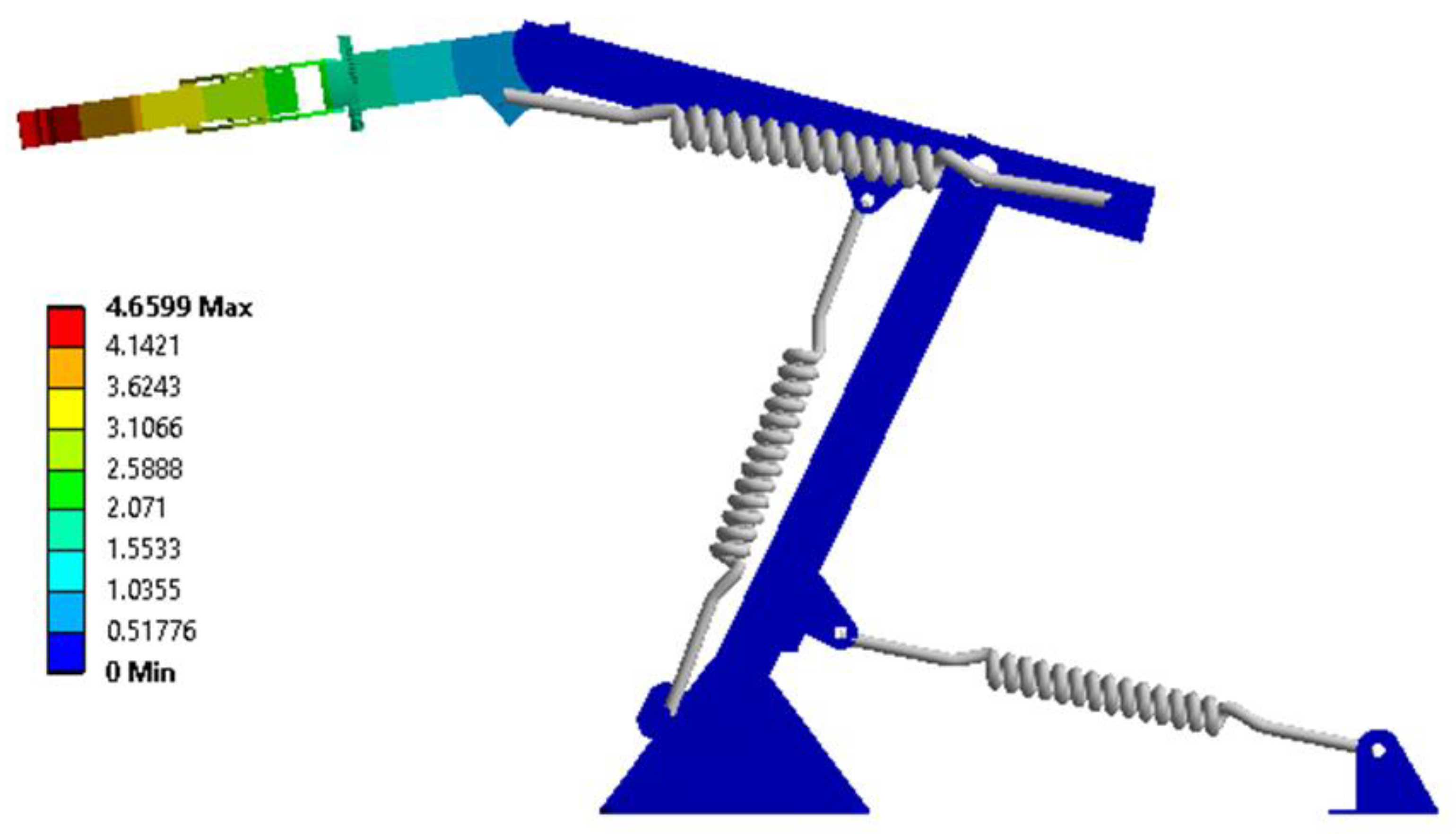
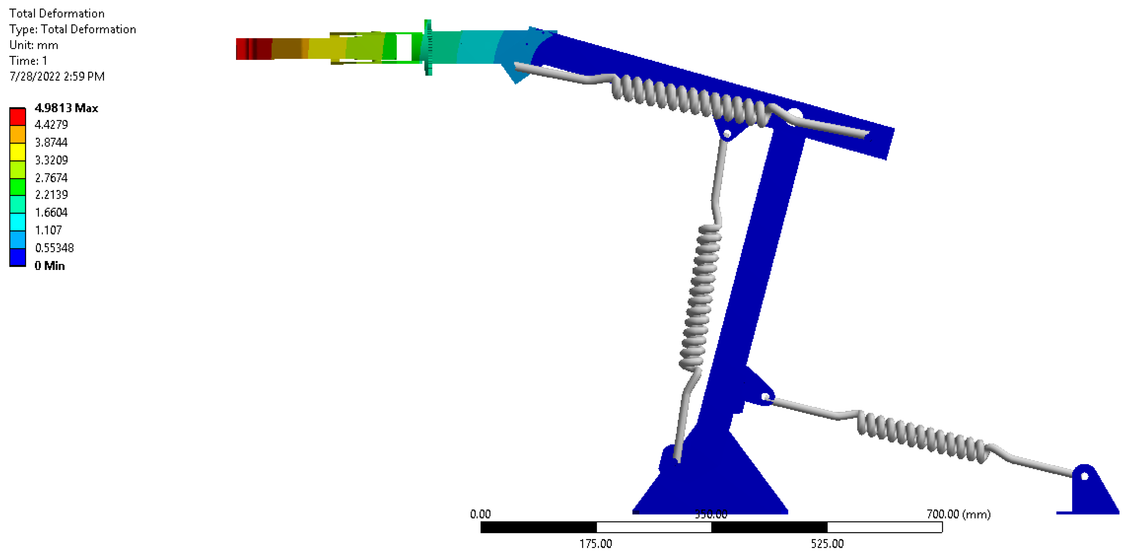
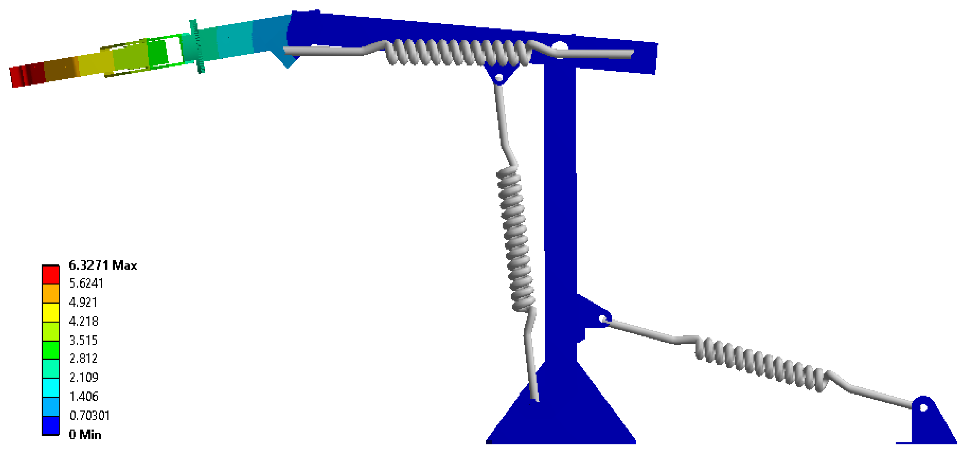
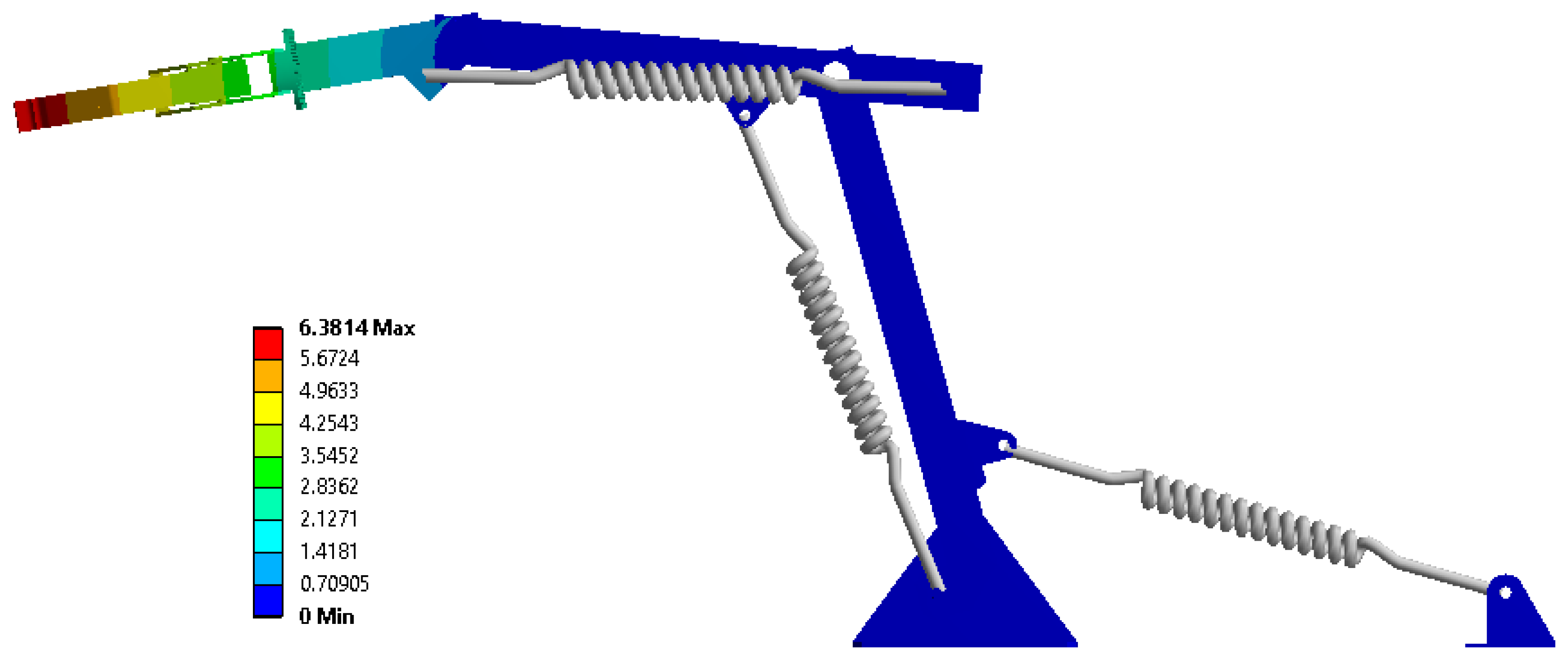
5. Numerical Modeling

The five geometric configurations of the robotic arm were modeled with FEM, using ANSYS software. In the first approach, “Bound”-type contacts were used between elements of the same arm or motor, and “Revolute”-type connections were used to shape the joints between the arms (Figure 11).

In place of the linear motors, we used elastic elements with an axial stiffness of 500 N/mm. As the elongations measured in the direction of the linear motors lead to a small vertical displacement of the final effector (gripper), under the action of the weight force the linear motors were replaced with linear springs in both the analytical and finite element models. We performed this calculation artificially, as the rigidity of these springs is reduced compared to that of the linear motors, and this allowed us to produce a model of the elasticity, obtained between the motor joints. Additionally, in the analytical–numerical model, we introduced the imperfections from the joints.

On the linear motor, there is a steel rod, with a diameter of 3 mm, used for stroke limiters. This rod was no longer represented, as it was not important to the elasticity of the system. As the geometric configuration does not allow the mounting of the displacement sensor between the axes of the joints, the solution in Figure 12 was adopted.

Figure 13 shows a discretization of the robotic arm for the case of geometric configuration 1. In total, 185,530 elements and 357,152 nodes were used.

The base was restricted in movement, and two concentrated forces were applied to the effector tanks 400 mm from the joint between arms 2 and 3 (the point of application of the force is O₄).

The static analysis resulted in the displacements for each case, and the results of the numerical analysis are presented in Figure 14, Figure 15, Figure 16, Figure 17 and Figure 18, with the voltages and all the quantities of interest.

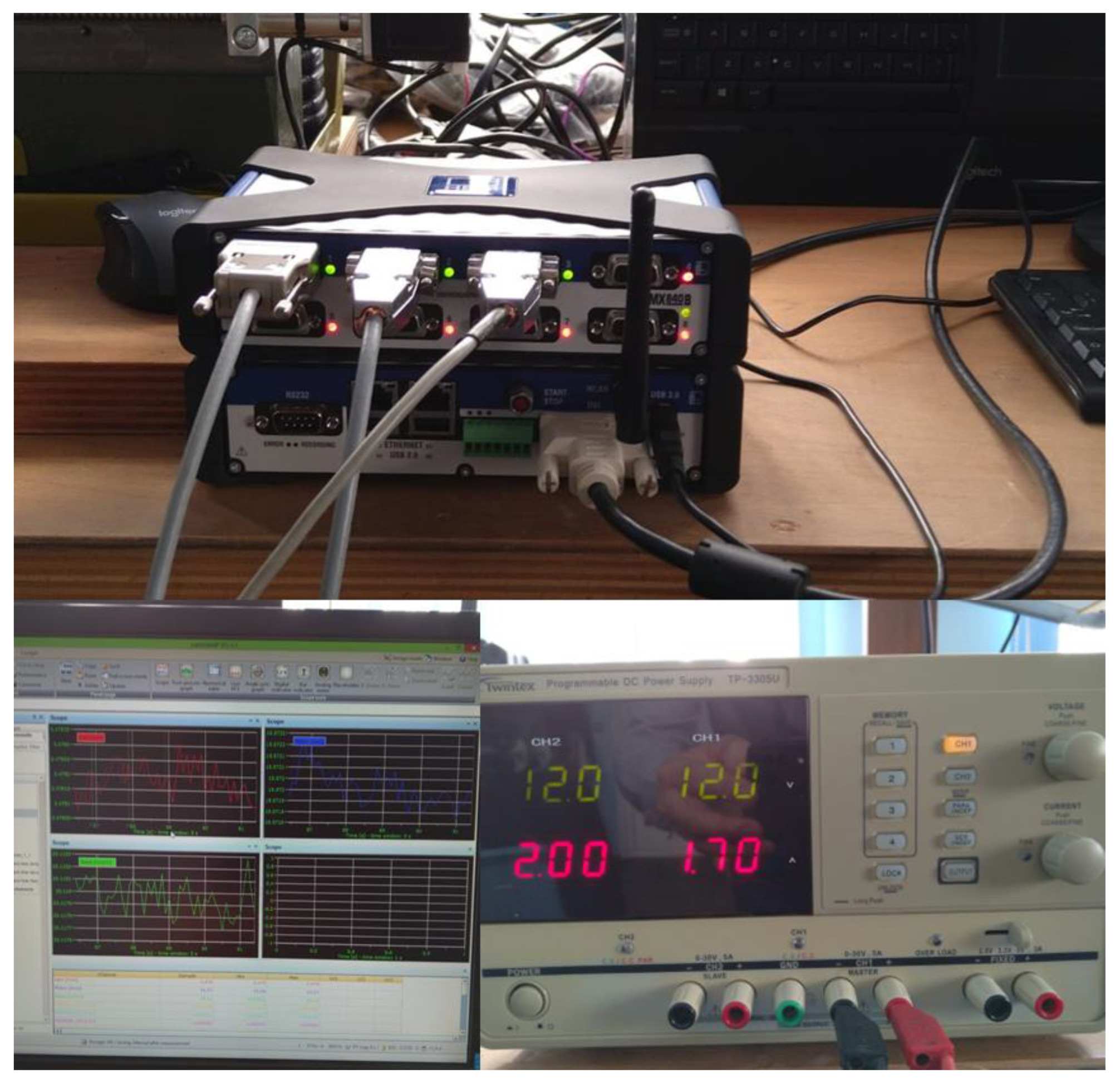
6. Experimental Results

The elasticity of the robotic arm with three degrees of freedom was analyzed experimentally, analytically, and numerically. For the experimental part, three masses were used: 1.5 kg, 5 kg, and 6.5 kg, which were applied to the effector of the robotic arm. Depending on the mass and the geometric configuration considered, vertical displacement of the effector was found, which was measured with the Baumer Electric CH-B501 laser displacement sensor.

HBM WA 200mm inductive displacement sensors were mounted between the fixed and movable parts of the linear motors. The sensors were connected to the QUANTUMX MX840B data acquisition bridge. Figure 19 shows the robot in the first position (configuration 1). The angles of the robot’s arms and the operating platform were measured with a robot.

The procedure for performing the experiments consisted of the following algorithm:

• The operation of the arm drive motors was checked independently and simultaneously.
• The load-bearing platform (chassis side with propeller) was in contact with the ground to ensure working conditions similar to those in the area of operations.
• To ensure that the center of gravity of the robot, at rest, was the same, 10 lifts were performed from the ground, and then the item was dropped from a height of 100 mm, finding that the games in the track, which is made from rubber, and the track tension system had a margin of error of 0.5 mm.
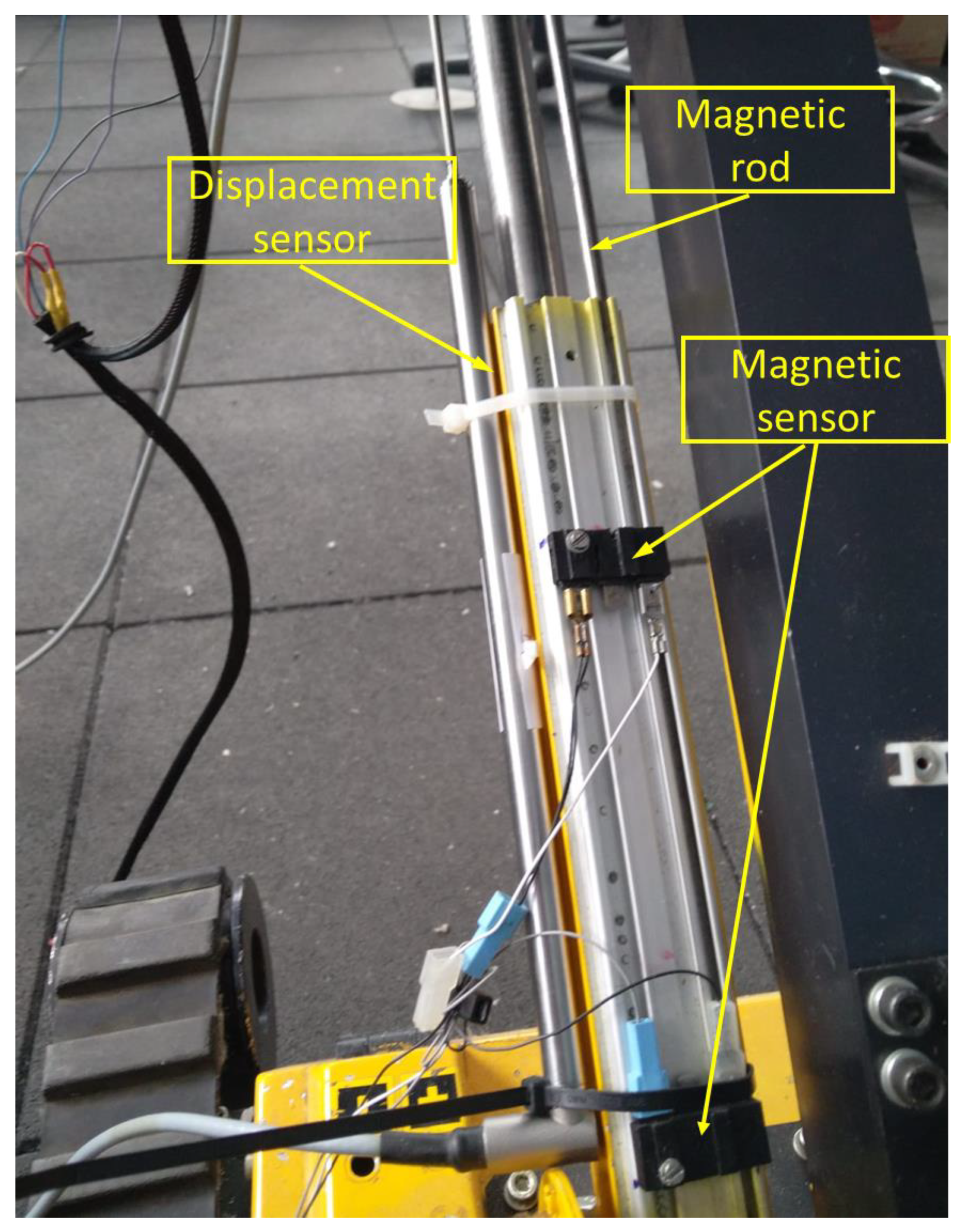
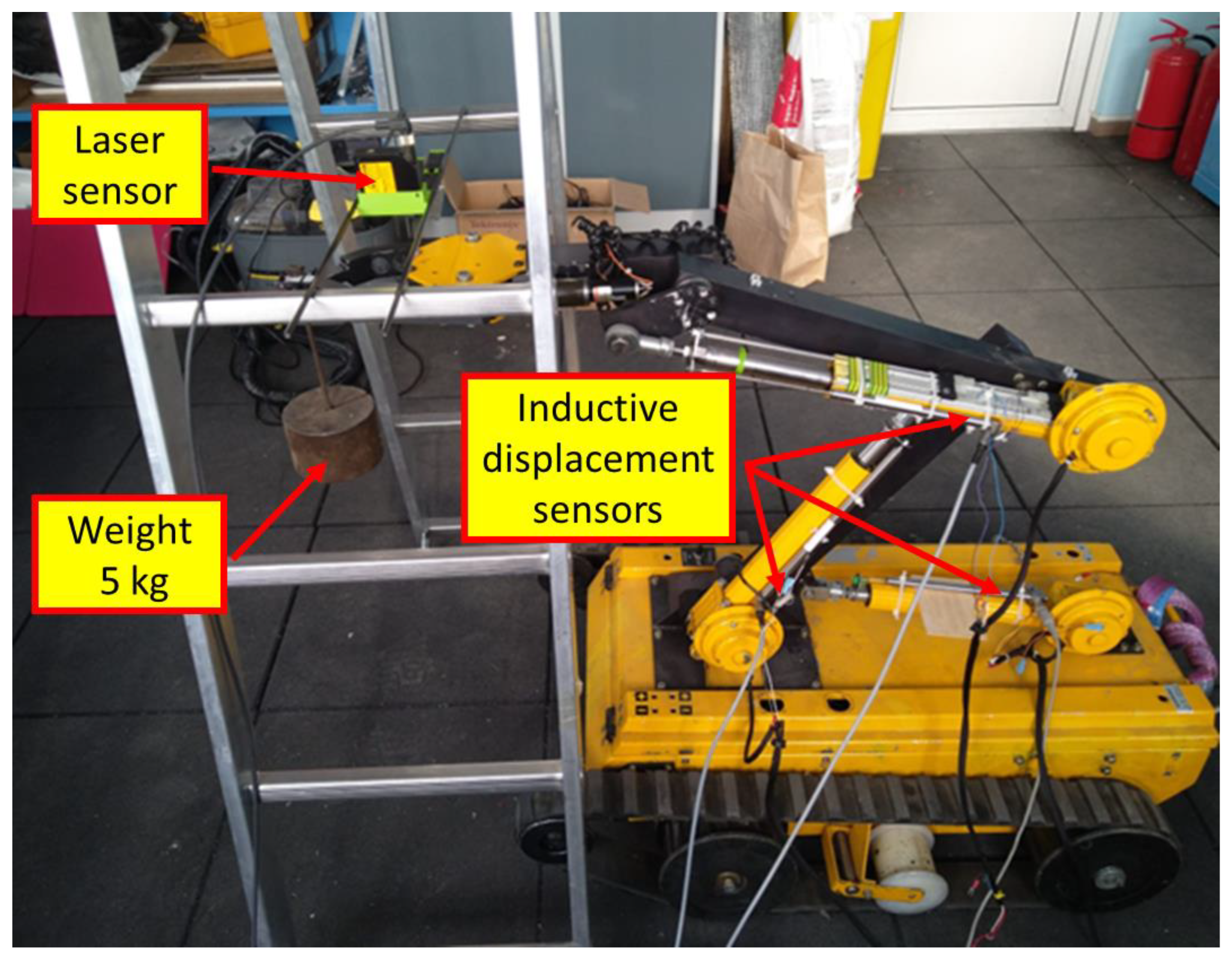
• Inductive displacement sensors were set to zero before each experimental determination.
• In the position corresponding to working configuration 1, with the laser sensor mounted, a forced vibration was induced around the final effector to check if the assembly returns to the initial position.
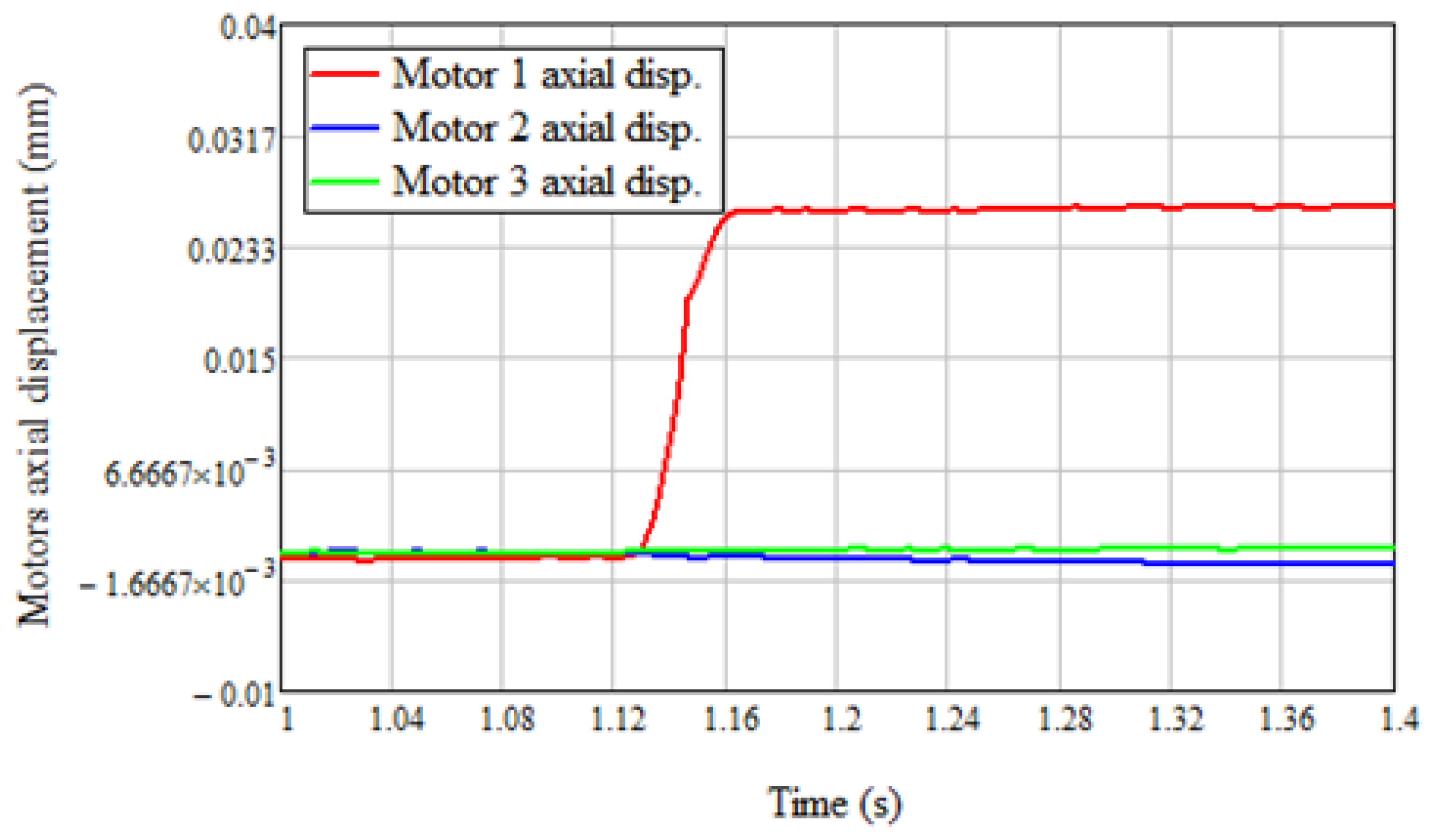
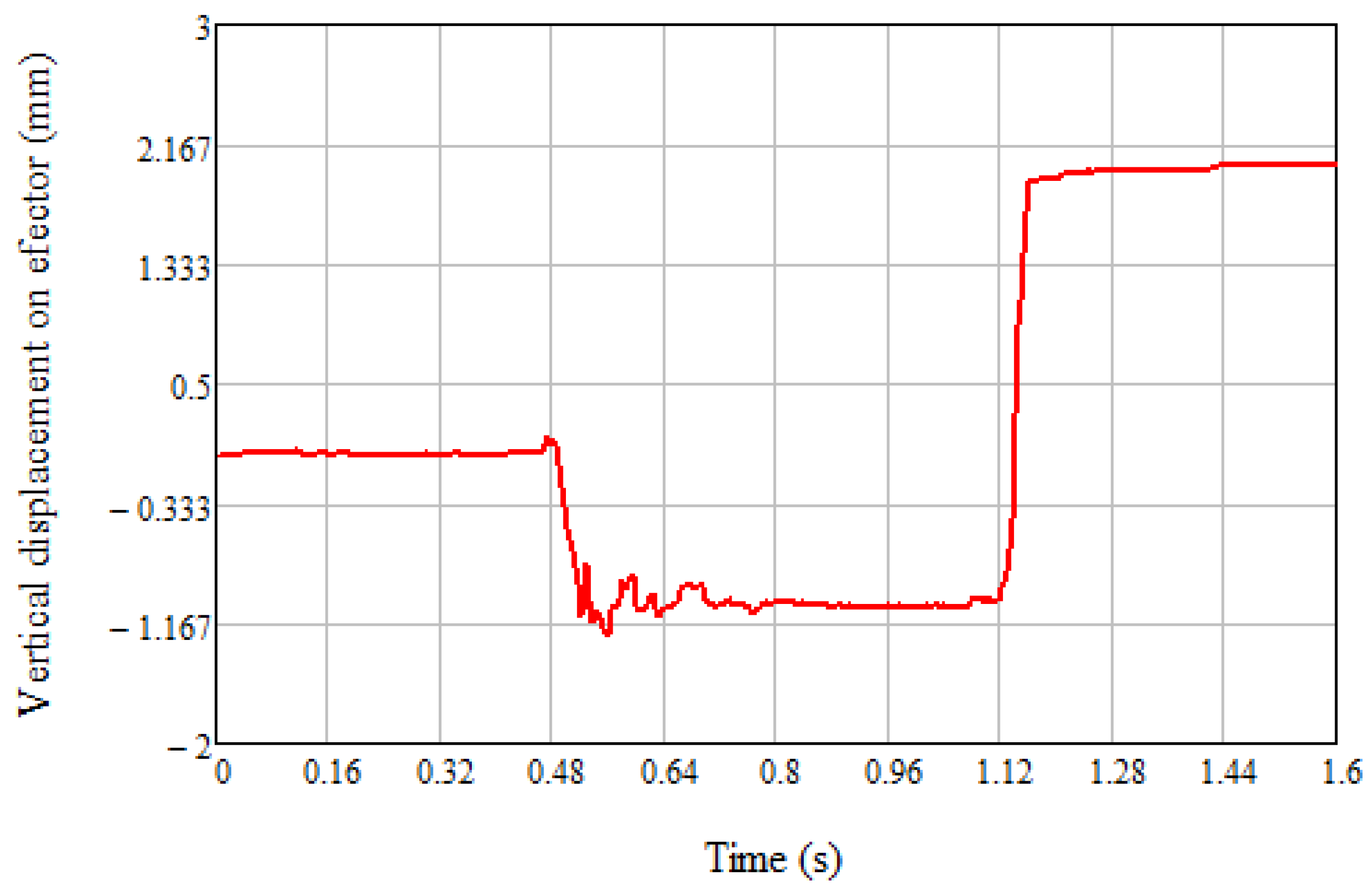
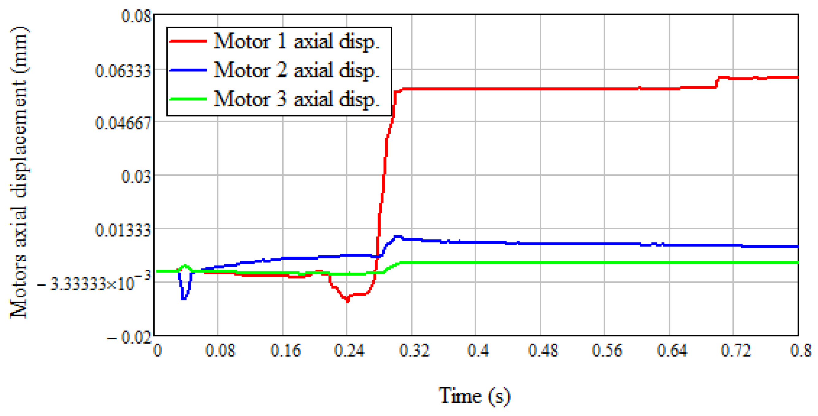
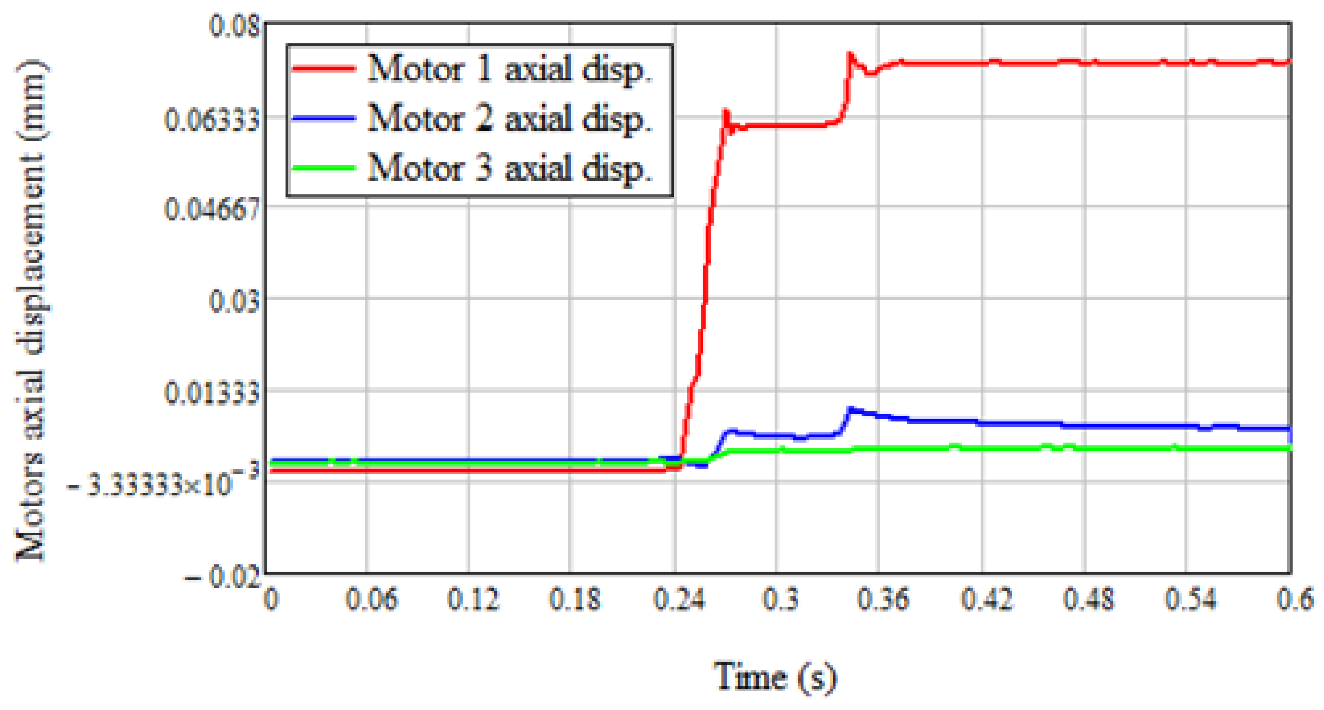
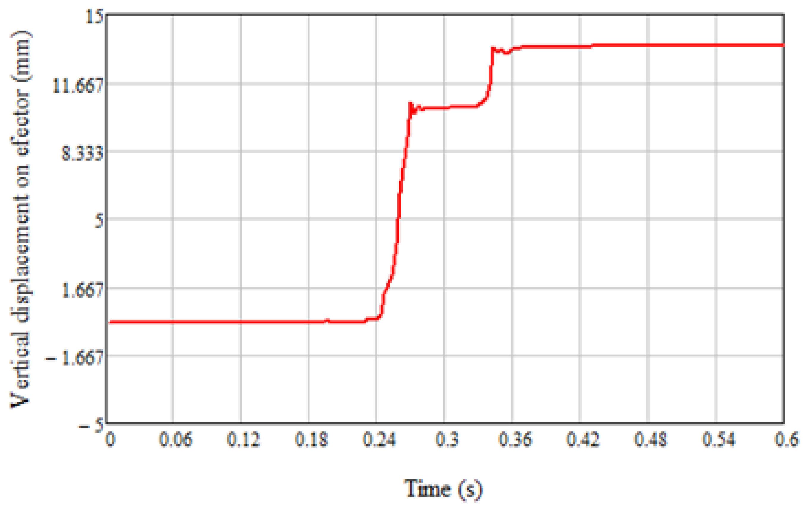
• For the experimental determinations of the displacements, the data acquisition was started, and, later, the weights that load the effector were added manually, placing them on the plate without shock. After stabilizing the signals, recording stopped (Figure 20). All data purchases were recorded with a frequency of 300Hz.

Figure 21, Figure 22, Figure 23, Figure 24, Figure 25 and Figure 26 show the variation in the axial displacement between the fixed and the moving part of the linear motors and the vertical displacement of the effector for the three cases of loading the effector for configuration 1, determined experimentally.

The beginning and end of the signal are truncated in the graphs, detailing the area co-responsible for the occurrence of displacement when applying weights. The variations in the displacements that appear before the one due to the application of the weight were produced by the manual action of the experimenter on the plate caught by the effector.

For the other configurations, the variations are similar, so the data of interest are presented in tabular form. After stabilizing the values over time, the displacements were mediated, resulting in the centralized values in

Table 3. Experimentally determined values of arm angles, for the five configurations, without a mass added to the effector and with a mass added.

		Arm Angle 1		Arm Angle 2		Arm Angle 3
		Without Mass	With Mass	Without Mass	With Mass	Without Mass	With Mass
Configuration 1	1.5 kg	115.6	115.5	15.4	15.2	0.2	0.1
	5 kg	115.6	115.2	15.4	14.7	0.2	−1.2
	6.5 kg	115.6	115.0	15.4	14.5	0.2	−1.7
Configuration 2	1.5 kg	104.7	105.7	15.7	15.1	0	−0.2
	5 kg	104.7	105.3	15.7	14.6	0	−0.9
	6.5 kg	104.7	105.2	15.7	14.6	0	−1.2
Configuration 3	1.5 kg	89.9	89.7	5.6	5.4	0.1	−0.1
	5 kg	89.9	89.6	5.6	5.1	0.1	−1.4
	6.5 kg	89.9	89.3	5.6	5.0	0.1	−1.6
Configuration 4	1.5 kg	74.8	74.7	5.8	5.6	0.4	−0.1
	5 kg	74.8	74.3	5.8	5.2	0.4	−1.1
	6.5 kg	74.8	74.2	5.8	5.0	0.4	−1.7
Configuration 5	1.5 kg	58.6	58.4	6.0	5.8	0.4	0.2
	5 kg	58.6	58.1	6.0	5.4	0.4	−1.0
	6.5 kg	58.6	58.0	6.0	5.2	0.4	−1.5

and

Table 4. Experimentally determined values of axial displacements in linear motors, and the vertical displacement of the effector, for the five configurations, after applying the masses to the effector.

	Table Loaded on Effector (kg)	Motor 1 (mm)	Motor 2 (mm)	Motor 3 (mm)	Vertical Effector Movement (mm)
Configuration 1	1.5	0.026	8.268 × 10−4	7.732 × 10−4	2.025
	5	0.0602	0.0074	0.0025	10.23
	6.5	0.0726	0.0063	0.0027	13.45
Configuration 2	1.5	0.0121	5.2591 × 10−5	6.3923 × 10−5	2.11
	5	0.034	0.0024	0.0025	8.22
	6.5	0.0441	0.0096	0.0019	11.47
Configuration 3	1.5	0.0142	0.0031	0.0019	2.88
	5	0.0336	0.0079	0.00023	12.05
	6.5	0.042	0.008	0.0001	14.31
Configuration 4	1.5	0.0136	0.0049	0.0002	3.02
	5	0.034	0.0019	0.00068	12.70
	6.5	0.032	0.0053	0	15.56
Configuration 5	1.5	0.0011	0.002	0	5.04
	5	0.0027	0.0025	0	9.50
	6.5	0.0038	0.0027	0.0002	11.43

, for the five working configurations.

Table 5. Axial forces in linear motors, calculated analytically with Relations (3), (5), and (8).

	Weight (kg)	Fm1 (N)	Fm2 (N)	Fm3 (N)
Configuration 1	1.5	−185.5	252.4	114.4
	5	−441.1	535.6	381.3
	6.5	−550.7	657	495.6
Configuration 2	1.5	−196.4	223.4	113.5
	5	−439.1	474.2	378.3
	6.5	−543.1	581.6	491.8
Configuration 3	1.5	−229.6	222	136.8
	5	−485.2	469.2	455.9
	6.5	−594.7	575.2	592.7
Configuration 4	1.5	−268.5	211.3	137.1
	5	−550.1	446.6	456.9
	6.5	−670.8	547.4	594
Configuration 5	1.5	−325.3	217.5	136.5
	5	−652.6	459.7	454.9
	6.5	−792.9	563.5	591.4

shows the results obtained for the five geometric configurations and three load cases, neglecting the weights of the arms and motors, using Relations (3), (5), and (8). Please note that the negative value is a motor tension request, and the positive value is a compression request.

From the geometric analysis of the experimental determinations, the vertical displacement of the effector under the action of gravity can be interpreted (in the case of arms with a rigid solid behavior) as being due to the rigid rotation of the robot arms due to the axial elasticity of the linear motors.

Table 6. Effector displacement calculated based on experimentally determined angles of the robot arms. All calculations were performed based on rigid solid rotations of the robot arms.

	Weight (kg)	Analytical Displacement Determined on the Basis of Experimental Values (Table 4) of Axial Displacements in Linear Motors (mm)	Experimentally Measured Displacement (mm)
Configuration 1	1.5	1.49	2.03
	5	10.55	10.23
	6.5	13.78	13.45
Configuration 2	1.5	7.37	2.11
	5	13.48	8.22
	6.5	14.82	11.47
Configuration 3	1.5	2.44	2.88
	5	11.34	12.05
	6.5	13.11	14.31
Configuration 4	1.5	4.24	3.02
	5	13.19	12.7
	6.5	17.95	15.56
Configuration 5	1.5	3.35	5.04
	5	13.79	9.5
	6.5	18.26	11.43

shows a comparison of the displacement of the point on the effector targeted by the laser sensor calculated based on the rotation of the arms and the one measured experimentally.

For configurations 1, 3, and 4, there is a concordance between values. An acceptable situation was found for configuration 4. Unsatisfactory results were obtained for configuration 2. If the axial deformations of the experimentally determined motors are considered, with the observation that linear motor 1 is stretched, the measured quantity is added to the distance between its joints, motors 2 and 3 are compressed, and the measured value decreases, as shown in

Table 7. Effector displacement calculated based on the axial deformation of the experimentally measured motors.

	Weight (kg)	The Displacement Determined Analytically Based on the Variation in the Angles of the Arms, the Angular Values Being Measured (mm)	Experimentally Measured Displacement (mm)
Configuration 1	1.5	0.203	2.03
	5	0.519	10.23
	6.5	0.602	13.45
Configuration 2	1.5	0.085	2.11
	5	0.272	8.22
	6.5	0.389	11.47
Configuration 3	1.5	0.143	2.88
	5	0.303	12.05
	6.5	0.364	14.31
Configuration 4	1.5	0.144	3.02
	5	0.292	12.7
	6.5	0.293	15.56
Configuration 5	1.5	0.024	5.04
	5	0.042	9.5
	6.5	0.056	11.43

.

It is noted that the elasticity of the motors does not explain the movement of the effector. The elasticity of the entire robotic arm is due to both the elasticity of the entire system and the play in the joints. If the direction of the motor’s elastic elements with an axial stiffness of 500 N/mm is considered, on the basis of Table 5, it is possible to calculate the changes in the lengths of the resulting displacements presented in

Table 8. Effector displacement calculated on the basis of the axial deformations of the motors, considering them as elastic elements.

	Weight (kg)	The Displacement Determined Analytically Based on the Variation in the Angles of the Arms, the Angular Values Being Measured (mm)	Experimentally Measured Displacement (mm)
Configuration 1	1.5	3.622	2.03
	5	9.679	10.23
	6.5	12.252	13.45
Configuration 2	1.5	2.716	2.11
	5	8.133	8.22
	6.5	10.433	11.47
Configuration 3	1.5	3.076	2.88
	5	10.375	12.05
	6.5	13.439	14.31
Configuration 4	1.5	1.816	3.02
	5	7.976	12.7
	6.5	10.553	15.56
Configuration 5	1.5	0.189	5.04
	5	4.853	9.5
	6.5	6.792	11.43

.

There is a good match of the results for configurations 1, 2, and 3 and a poor match for configurations 4 and 5.

Table 9. Effector displacement calculated based on the axial deformations of the motors, considering them as elastic elements by the analytical method, and numerically and experimentally measured displacements.

	Weight (kg)	Analytical Displacement Determined by Engine Elasticity not Determined Analytically (mm)	Analytically Determined Displacement Based on Numerically Determined Engine Elasticity (FEM) (mm)	Experimentally Measured Displacement (mm)
Configuration 1	1.5	3.622	3.052	2.03
	5	9.679	11.26	10.23
	6.5	12.252	13.227	13.45
Configuration 2	1.5	2.716	3.349	2.11
	5	8.133	11.163	8.22
	6.5	10.433	14.512	11.47
Configuration 3	1.5	3.076	4.133	2.88
	5	10.375	13.778	12.05
	6.5	13.439	17.91	14.31
Configuration 4	1.5	1.816	4.11	3.02
	5	7.976	13.17	12.7
	6.5	10.553	17.81	15.56
Configuration 5	1.5	0.189	4.51	5.04
	5	4.853	15.05	9.5
	6.5	6.792	19.56	11.43

shows the comparative analytical, numerical, and experimental results for the displacement of the point on the effector and the displacement measured near the measuring point of the laser sensor.

There is a better match between the numerically calculated and experimentally determined values for configurations 1 to 4.

7. Conclusions

Elasticity manifested in all the components of the robotic arm, but with preponderance in the axial direction of the linear motors, in the articulation area between the motor and the robotic arm. The significant influence of the movement of the effector under the action of some weights was due to the games in the joint. After the experimental and theoretical analysis, the joints were untied, and a play was noticed that was mainly due to wear, which varied between 0.1 and 0.3 mm. The largest deviation was found in the joint between arms 2 and 3. These deviations led to positioning errors of the robotic arm. The transition from the positive to the negative quadrant of the vertical oscillations of the final effector had an arbitrary law of motion. Another aspect is the deformation of the robotic arm in space.

The calculations omitted the elasticity of the chassis and the locomotion system, which also influences the movement of the effector. In the analytical and numerical calculations, the geometry in the joint area was considered to be perfectly cylindrical, that is, any wear that was unevenly distributed in the joints was omitted. The high axial stiffness of the linear motors was noticeable.

Although there are substantial uncertainties in current theoretical and computational models regarding the prediction of the evolution of the elastic state of mechanical elements for mobile robots, the simulation responded quite well to the real conditions. Regarding the deviations, the following can be concluded:

• It was observed following the experimental research that, in certain situations, if the effector was loaded with a certain force of weight, after its removal, the effector did not return to the initial position, which confirms the presence of deviations in the joints of the robotic arm;
• Due to these deviations, estimating the evolution of the effector element is difficult in certain operating conditions: certain arm openings and certain loads;
• The effects of deviations can be remedied by performing maintenance operations.

Many of the limitations of the existing solution have already been mentioned; in addition to these, we consider that limitations may also occur due to the abilities of EOD robot operators. Additionally, in the next article, we will present an analysis of the free vibrations of the robotic arm. The study will follow the data that will be obtained experimentally for multiple work configurations with and without loads.

For the study of free vibrations, the experimental analysis formula will be completed with accelerometers placed on each component of the robotic arm. After that, our attention will be directed toward the investigation of the dynamic response that occurs when a certain mass is manipulated by a robotic arm. One of our goals is to determine what types of structural modifications may lead to a reduction in the amplitude of vibrations experienced by the robotic arm. Another area of research may be the investigation of the dynamic reaction of the robotic arm when it is loaded with a weight.

In order to continue our research on the functioning of the robotic arm, we will investigate the effect of vibrations on the positioning accuracy of the end effector. We will also examine the dynamic reaction to the movement of a loaded arm with a weight on a fixed platform. If the weight is an explosive artisanal device and the level of the vibration amplitude is high, it can detonate. The final investigation will be to analyze the operation of the arm while moving the robot.

References

1. Zhao, J.; Han, T.; Ma, X.; Ma, W.; Liu, C.; Li, J.; Liu, Y. Research on Kinematics Analysis and Trajectory Planning of Novel EOD Manipulator. Appl. Sci. 2021, 11, 9438. [Google Scholar] [CrossRef]
2. Tavsel, O. Mechatronic Design of an Explosive Ornance Disposal Robot. Master’s Thesis, Izmir Institute of Technology, Urla, Turkey, June 2005. [Google Scholar]
3. Lopatka, M.J.; Sterniczuk, D. Concept of the manipulators set for fast IEDs neutralization. AIP Conf. Proc. 2018, 2029, 020037. [Google Scholar]
4. Wells, P.; Deguire, D. TALON: A universal unmanned ground vehicle platform, enabling the mission to be the focus. Proc. SPIE 2005, 5804. [Google Scholar] [CrossRef]
5. Nuță, I.; Orban, O.; Grigore, L.Ș. Development and improvement of technology in emergency response. Procedia Econ. Financ. 2015, 32, 603–609. [Google Scholar] [CrossRef] [Green Version]
6. Peskoe-Yang, L. Paris Firefighters Used This Remote-Controlled Robot to Extinguish the Notre Dame Blaze. IEEE Spectrum, 22 April 2019. [Google Scholar]
7. Raghavendran, P.S.; Suresh, M.; Ranjith Kumar, R.; Ashok Kumar, R.; Mahendran, K.; Swathi, S.; Kamesh, L.; Sanjay, R. An Intelligent Remote-Controlled Fire Fighting Machine for Autonomous Protection of Human being. Int. J. Adv. Res. Sci. Eng. Technol. 2018, 5, 7620–7626. [Google Scholar]
8. Wang, W.; Gao, W.; Zhao, S.; Cao, W.; Du, Z. Robot Protection in the Hazardous Environments: Chapter 4; InTechOpen: London, UK, 2017. [Google Scholar]
9. Constantin, D.; Toma, V. TVF-1: Experimental Model of an EOD Robot. J. Mil. Technol. 2018, 1, 51–56. [Google Scholar] [CrossRef]
10. Grigore, L.Ș.; Holban-Oncioiu, I.; Priescu, I.; Joița, D. Development and Evaluation of the Traction Characteristics of a Crawler EOD Robot. Appl. Sci. 2021, 11, 3757. [Google Scholar] [CrossRef]
11. Carey, M.W.; Kurz, E.M.; Matte, J.D.; Perrault, T.D. Novel EOD Robot Design with a Dexterous Gripper and Intituitive Teleoperation. In Proceedings of the World Automation Congress 2012, Puerto Vallarta, Mexico, 24–28 June 2012; Volume 1, pp. 463–469. [Google Scholar]
12. Gubankov, A.; Yukhimets, D. Development and Experimental Studies of an Identification Method of Kinematic Parameters for Industrial Robots without External Measuring Instruments. Sensors 2022, 22, 3376. [Google Scholar] [CrossRef]
13. Renders, J.M.; Rossignol, E.; Becquet, M.; Hanus, R. Kinematic calibration and geometrical parameter identification for robots. IEEE Trans. Robot. Autom. 1991, 7, 721–732. [Google Scholar] [CrossRef]
14. Pratheep, V.G.; Chinnathambi, M.; Priyanka, E.B.; Ponmurugan, P.; Thiagarajan, P. Design and Analysis of six DOF Robotic Manipulator. IOP Conf. Ser. Mater. Sci. Eng. 2021, 1055, 012005. [Google Scholar] [CrossRef]
15. Zeng, J.J.; Yang, R.Q.; Zhang, W.J.; Weng, X.H.; Qian, J. Research on Semi-automatic Bomb Fetching for an EOD Robot. Int. J. Adv. Robot. Syst. 2007, 4, 247–252. [Google Scholar]
16. De Cubber, G.; Balta, H.; Lietart, C. Teodor: A semi-autonomous search and rescue and demining robot. Appl. Mech. Mater. 2014, 658, 599–605. [Google Scholar] [CrossRef]
17. Kruzic, S.; Music, J.; Kamnik, R.; Papic, V. End-Effector Force and Joint Torque Estimation of a 7-DoF Robotic Manipulator Using Deep Learning. Electronics 2021, 10, 2963. [Google Scholar] [CrossRef]
18. Zhang, H.; Zhu, Y.; Liu, X.; Xu, X. Analysis of Obstacle Avoidance Strategy for Dual-Arm Robot Based on Speed Field with Improved Artificial Potential Field Algorithm. Electronics 2021, 10, 1850. [Google Scholar] [CrossRef]
19. Colucci, G.; Botta, A.; Tagliavini, L.; Cavallone, P.; Baglieri, L.; Quaglia, G. Kinematic Modeling and Motion Planning of the Mobile Manipulator Agri.Q for Precision Agriculture. Machines 2022, 10, 321. [Google Scholar] [CrossRef]
20. Hegedűs, T.; Németh, B.; Gáspár, P. Design of a Low-complexity Graph-Based Motion-Planning Algorithm for Autonomous Vehicles. Appl. Sci. 2020, 10, 7716. [Google Scholar] [CrossRef]
21. Grigore, L.Ș.; Ileri, R.; Neculăescu, C.; Soloi, A.; Ciobotaru, T.; Vînturis, V. A class of autonomous robots prepared for unfriendly sunny environment. In Proceedings of the CAR2011—2011 3rd International Asia Conference on Informatics in Control, Automation and Robotics, Xiamen, China, 25–26 June 2011; Volume 646. [Google Scholar]
22. Wong, J. Theory of Ground Vehicle, 2nd ed.; John Willey & Sons: New York, NY, USA, 1993; ISBN 13:978-0-470-17038-0. [Google Scholar]
23. Wong, J.Y.; Chiang, C.F. A general theory for skid steering of tracked vehicles. J. Automob. Eng. 2001, 215, 343–355. [Google Scholar] [CrossRef]
24. Balestrieri, E.; Daponte, P.; De Vito, L.; Lamonaca, F. Sensors and Measurements for Unmanned Systems: An Overview. Sensors 2021, 21, 1518. [Google Scholar] [CrossRef]
25. Odedra, S.; Prior, S.D.; Karamanoglu, M. Investigating the Mobility of Unmanned Ground Vehicles. In Proceedings of the International Conference on Manufacturing and Engineering Systems, Huwei, Taiwan, 17–19 December 2009. [Google Scholar]
26. Manish, R.; Lin, Y.C.; Ravi, R.; Hasheminasab, S.M.; Zhou, T.; Habib, A. Development of a Miniaturized Mobile Mapping System for In-Row Under-Canopy Phenotyping. Remote Sens. 2021, 13, 276. [Google Scholar] [CrossRef]
27. Reina, G.; Milella, A.; Underwood, J. A self-Learning Ground Classifier Using Radar Features. In Field and Service Robotics; Springer: Berlin/Heidelberg, Germany; pp. 629–642.
28. Im, G.; Kim, M.; Park, J. Parking Line Based SLAM Approach Using AVM/LiDAR Sensor Fusion for Rapid and Accurate Loop Closing and Parking Space Detection. Sensors 2019, 19, 4811. [Google Scholar] [CrossRef] [Green Version]
29. Zhang, X.; Wang, W.; Qi, X.; Liao, Z.; Wei, R. Point-Plane SLAM Using Supposed Planes for Indoor Environments. Sensors 2019, 19, 3795. [Google Scholar] [CrossRef] [PubMed] [Green Version]
30. Olmedo, N.A.; Barczyk, M.; Zhang, H.; Wilson, W.; Lipsett, M.G. A UGV-based modular robotic manipulator for soil sampling anf terramechanics investigation. J. Unmanned Veh. Syst. 2020, 8, 364–381. [Google Scholar] [CrossRef]
31. Velaskar, P.; Vargas-Clara, A.; Jameel, O.; Redkar, S. Guided Navigation Control of an Unmanned Ground Vehicle using Global Positioning Systems and Inertial Navigation Systems. Int. J. Electr. Comput. Eng. 2014, 4, 329–342. [Google Scholar] [CrossRef]
32. Muppidi, S. Development of a Low-Cost Controller and Navigation System for Unmanned Ground Vehicle. Master’s Thesis, West Virginia University, Morgantown, WV, USA, 2008; p. 152. [Google Scholar]
33. Jaimes, A.; Gonzalez, J.; Ibarra, A.; Benavidez, P.; Jamshidi, M. Low-Cost Heterogeneous Unmanned Ground Vehicle (UGV) Testbed for Systems of Autonomous Vehicles Research. In Proceedings of the 14th Annual Conference System of Systems Engineering (SoSE), Anchorage, AK, USA, 19–22 May 2019; p. 18819465. [Google Scholar]
34. Murtaza, Z.; Mehmood, N.; Jamil, M.; Ayaz, Y. Design and implementation of low cost remote-operated unmanned ground vehicle (UGV). In Proceedings of the International Conference on Robotics and Emerging Allied Technologies in Engineering (ICREATE), Islamabad, Pakistan, 22–24 April 2014. [Google Scholar]
35. Kwet, C.; Lam, Y.; Man, L.; Koonjul, Y.; Nagowah, L. A low cost autonomous unmanned ground vehicle. Future Comput. Inform. J. 2018, 3, 304–320. [Google Scholar]
36. Berns, K.; Nezhadfard, A.; Tosa, M.; Balta, H.; De Cubber, G. Unmanned Ground Robots for Rescue Tasks: Chapter 4; InTechOpen: London, UK, 2017. [Google Scholar]
37. Ding, Z.; Li, Y.; Tang, Z. Theoretical Model for Prediction of Turning Resistance of Tracked Vehicle on Soft Terrain. Hindawi Math. Probl. Eng. 2020, 2020, 4247904. [Google Scholar] [CrossRef]
38. Chen, K.; Kamezaki, M.; Katano, T.; Azuma, K.; Ishida, T.; Seki, M.; Ichiryu, K.; Sugano, S. Compound locomotion control system combining crawling and walking for multi-crawler multi-arm robot to adapt unstructured and unknown terrain. ROBOMECH J. 2018, 5, 2. [Google Scholar] [CrossRef] [Green Version]
39. Laska, P.R. Bombs, IEDs, and Explosives. Identification, Investigation and Disposal Techniques; CRC Press: Boca Raton, FL, USA, 2015; ISBN 9781498714501. [Google Scholar]
40. Lundberg, C. Assessment and Evaluation of Man-portable Robots for High-risk Professions in Urban Settings. Ph.D. Thesis; KTH School of Computer Science and Communication: Sweden, 2007. Available online: http://kth.diva-portal.org/smash/record.jsf?pid=diva2%3A12748&dswid=3243 (accessed on 20 January 2022).
41. Grigore, L.Ș.; Priescu, I.; Grecu, D.L. Applied Artificial Intelligence in Fixed and Mobile Robotic Systems. Cap 4 Terrestrial Mobile Robots; AGIR: Bucharest, Romania, 2020; ISBN 978-973-72-0767-8. [Google Scholar]
42. Wu, Q.; Chen, Z.; Wang, L.; Lin, H.; Jiang, Z.; Li, S.; Chen, D. Real-Time Dynamic Path Planning of Mobile Robots: A Novel Hybrid Heuristic Optimization Algorithm. Sensors 2020, 20, 188. [Google Scholar] [CrossRef] [PubMed] [Green Version]
43. Trevelyan, J.P.; Kang, S.C.; Hamel, W.R. Robotics in Hazardous Applications. In Springer Handbook of Robotics; Siciliano, B., Khatib, O., Eds.; Springer: Berlin/Heidelberg, Germany, 2008. [Google Scholar] [CrossRef]
44. Kalajahi, E.G.; Mahboubkhah, M.; Barari, A. Numerical Versus Analytical Direct Kinematics in a Novel 4-DOF Parallel Robot Designed for Digital Metrology. In Proceedings of the 17th IFAC Symposium on Information Control Problems in Manufacturing INCOM 2021, Budapest, Hungary, 7–9 June 2021; Volume 54, pp. 181–186. [Google Scholar] [CrossRef]
Figure 1. The analyzed EOD robot.
Electronics 11 02355 g001
Figure 2. The analyzed EOD robot and the hook for positioning the working weights.
Electronics 11 02355 g002
Figure 3. Schematic representation of the robotic arm with the connection points and the association of this structure with some hydraulic cylinders.
Electronics 11 02355 g003
Figure 4. Schematic representation of the local coordinate system of arm no. 1.
Electronics 11 02355 g004
Figure 5. Schematic representation of the local coordinate system of arm no. 2.
Electronics 11 02355 g005
Figure 6. Schematic representation of the local coordinate system of arm no. 3.
Electronics 11 02355 g006
Figure 7. Schematic representation of the angular measuring system.
Electronics 11 02355 g007
Figure 8. Three-dimensional representation of the robotic arm, for which arm 3 was determined to remain in a horizontal position. These inclinations of arms 1 and 2 while keeping arm 3 in a horizontal position are intended to allow the measurement of the vertical displacements of the effector element, measured by means of a laser sensor. The angular orientation of the different working configurations can be found in Table 2.
Electronics 11 02355 g008
Figure 9. The representation of the two fixed and mobile coordinate systems is necessary for the schematic description of the analytical calculation algorithm.
Electronics 11 02355 g009
Figure 10. Representation of how the arms of the robot were isolated to perform the analytical calculations.
Electronics 11 02355 g010
Figure 11. In this figure, we show the representation (cross-section) of a linear motor. A brushless DC motor drives the screw. By means of the worm gear–worm wheel, the movement is transmitted to the ball screw that acts on the nut, removing or bringing the left joint closer to the right one.
Electronics 11 02355 g011
Figure 12. The robotic arm opening control system, which is composed of a magnetic rod to limit the stroke of the linear motor; it moves between the two magnetic sensors to control the stroke of the linear motor, so that the power supply of the motor can be stopped.
Electronics 11 02355 g012
Figure 13. Representation of the finite element model in which the linear motors are replaced by elastic elements.
Electronics 11 02355 g013
Figure 14. The resulting displacement field for configuration 1 and a force of 15 N.
Electronics 11 02355 g014
Figure 15. The resulting displacement field for configuration 2 and a force of 15 N.
Electronics 11 02355 g015
Figure 16. The resulting displacement field for configuration 3 and a force of 15 N.
Electronics 11 02355 g016
Figure 17. The resulting displacement field for configuration 4 and a force of 15 N.
Electronics 11 02355 g017
Figure 18. The resulting displacement field for configuration 5 and a force of 15 N.
Electronics 11 02355 g018
Figure 19. Representation of how the instrumentation was performed.
Electronics 11 02355 g019
Figure 20. Detail of the experiments.
Electronics 11 02355 g020
Figure 21. Time variations of axial deformations for the mass of 1.5 kg. The average values of the displacements after the application of the weight were calculated in the time interval (1.3, 1.4) s.
Electronics 11 02355 g021
Figure 22. Vertical displacement variations for the 1.5 kg mass. The negative displacement is due to the operator who held the plate rod with one hand and applied the weight to the plate with the second hand. The final displacement (mediated in the interval (1.3, 1.4) s) was determined from the mean value in the time interval (0, 0.4) s, considered to be zero.
Electronics 11 02355 g022
Figure 23. Time variations of axial deformations for the mass of 5 kg. The variation in the displacements for a time less than 0.28 s was due to the manual actuation.
Electronics 11 02355 g023
Figure 24. Vertical displacement variations for the 5 kg mass. The average values of the displacements were calculated in the time interval (0.72, 0.8) s.
Electronics 11 02355 g024
Figure 25. Time variations of axial deformations for the mass of 6.5 kg. The variation in the displacement when applying the two weights can be noticed. Approximately at time 0.27 s, a mass of 5 kg was applied, and at time 0.34 s, a mass of 1.5 kg was added.
Electronics 11 02355 g025
Figure 26. Vertical displacement variations for the 6.5 kg mass. The average values of the displacements were calculated in the time interval (0.48, 0.6) s.
Electronics 11 02355 g026