Effective Parametrization of Low Order Bézier Motion Primitives for Continuous-Curvature Path-Planning Applications

Abstract

We propose a new parametrization of motion primitives based on Bézier curves that suits perfectly path-planning applications (and environment exploration) of wheeled mobile robots. The individual motion primitives can simply be calculated taking into account the requirements of path planning and the constraints of a vehicle, given in the form of the starting and ending orientations, velocities, turning rates, and curvatures. The proposed parametrization provides a natural geometric interpretation of the curve. The solution of the problem does not require optimization and is obtained by solving a system of simple polynomial equations. The resulting planar path composed of the primitives is guaranteed to be $C^2$ continuous (the curvature is therefore continuous). The proposed primitives feature low order Bézier (third order polynomial) curves. This not only provides the final path with minimal required turns or unwanted oscillations that typically appear when using higher-order polynomial primitives due to Runge’s phenomenon but also makes the approach extremely computationally efficient. When used in path planning optimizers, the proposed primitives enable better convergence and conditionality of the optimization problem due to a low number of required parameters and a low order of the polynomials. The main contribution of the paper therefore lies in the analytic solution for the third-order Bézier motion primitive under given boundary conditions that guarantee continuous curvature of the composed spline path. The proposed approach is illustrated on some typical scenarios of path planning for wheeled mobile robots.

1. Introduction

Autonomous or guided mobile systems require path planning to find a path that allows the system to move safely from a starting configuration to a desired goal configuration. Finding a globally optimal, safe, and feasible path, given the driving constraints is a complex process that requires some kind of discretisation over the continuum of the configuration space. This makes it possible to compute a path plan in the limited time that satisfies the real-time requirements such as self-driving cars that need to react and replan their path promptly according to traffic changes [1,2].

In addition to the discretisation of time, which is essential in computer-aided design, space must also be discretised to a final number of possible configurations. Typically, regular grid-based environment discretisations are used, where the resulting path is a sequence of straight-line segments with discontinuities in the tangents and curvatures in the joints. For mobile systems such as wheeled robots with kinematic constraints, motion primitives provide a more flexible discretisation and better performance in sampling-based planning algorithms [2,3,4,5,6,7]. Motion primitives can consist of precomputed motions or curves with predefined (parametric) structure such as circular arcs, polynomials and the like.

Path planning can be reactive or cognitive. The former responds to local sensor readings (e.g., ultrasonic sensor, laser range camera, or visual sensors) and reschedules actions to avoid collisions using potential field methods, reactive controllers such as model predictive control, dynamic window approaches, or trajectory roll-out algorithms [8,9,10]. The latter rely on global environment information available in the form of an environment map and use roadmap or grid-based planners (such as A${}^{*}$, D${}^{*}$) [1,2], random sampling-based planners [11,12], and others. As the number of tuning parameters and the complexity of path planning algorithms (e.g., multi-robot planning) increases, various artificial intelligence methods are gaining popularity [13], such as reinforcement learning, Gaussian mixture models, neural networks, and others. The rest of the introduction and this paper focuses on path planning with motion primitives, which provide a basic type of smooth transitions in planning and environment exploration.

Paths or trajectories combined from motion primitives must be continuous to the k-th derivative ($C^k$) in the joints to satisfy vehicle driving constraints. Continuity may be geometric (e.g., continuity of curvature) or parametric (e.g., continuity of time derivatives of the trajectory). The former is more general and includes the latter. The path determined in the planning process must be consistent with the kinematic constraints of the vehicle, which usually include geometric continuity requirements [2,14,15]. When this path is driven by a vehicle, the time dimension is also included (resulting in a trajectory), which must also take into account the dynamic constraints of the vehicle, such as the maximum permissible velocity, acceleration, or jerk [16,17,18]. Trajectory planning includes path planning and velocity profile planning and is therefore even more complex. Therefore, a path-velocity decomposition is typically applied, where in the second step admissible velocity profiles are determined that meet time-related requirements such as minimising travel time or optimising driving comfort, while taking into account dynamic constraints on a predefined path [16,19,20].

A pioneering work constructing the shortest curvature-constrained path with straight-line segments and circular arcs for a vehicle with steering constraints was proposed by [21]. Such paths (Dubins or Reeds-Shepp’s) provide only geometric continuity of tangency while the curvature in the joints is discontinuous. Several extensions of these basic motion primitives have been proposed to obtain continuous curvature by inserting clothoid transitions [22] and similar smoothing approaches. Other popular parametric and non-parametric motion primitives with continuous curvature in the joints are clothoids [23,24], Bézier curves [5,14,17,18,25,26], B-splines [27], or higher order polynomials [15,28,29].

Among the alternatives mentioned for the construction of motion primitives, the Bernstein–Bézier polynomials are among the most commonly used. It was first introduced by S.N. Bernstein in 1912 and later enjoyed great popularity in computer-aided geometric design and also in other applications such as motion planning [30]. Its popularity is mainly due to its mathematical description, which is compact and intuitive and allows for elegant parameterisation. Several extensions of the classical Bézier curves were proposed to overcome some limitations of their fixed structures by introducing additional parameters for controlling curve shape [31,32,33]. In applications for mobile systems, it is typically used for exploring the environment, constructing lattice graphs for path planning [5,34,35,36], randomized (e.g., RRT) planner [11], path smoothing [37], or as a local planner [38] for connecting a given start and goal configuration or series of waypoints.

Objectives Furthermore, Contributions

In this work, we propose a new parametrisation of low-order (third order) Bézier motion primitives with continuous curvature (i.e., $C^2$ geometric curve continuity) in joints. The main innovations of the approach are as follows:

• Based on the findings of our literature review this is one of the few if not the first approach that apply third order Bézier curve motion primitives in path planning and takes into account the given requirements for initial and final position, orientation and curvature. The combined path using the proposed primitives has minimal required turns or oscillations between the initial and final configurations, since only a third order curve is used. Due to the small number of required parameters, the method is also suitable for use in path planning optimisers, since it reduces computational effort and improves convergence.
  Previous works from path planning area typically use higher order Bézier curves to satisfy $C^2$ continuity requirements, such as seventh order in [11], fifth order in [5,25,26,38,39], or fourth order in [17,36,37].
• We provide a new parametrization that allows an intuitive geometric interpretation of the curve and a simple algorithm to calculate its parameters. Parametrization is based on the initially available information, i.e., the position, orientation, and curvature requirements in the endpoints. The problem is solved by solving a system of two quadratic polynomial equations without the need for optimisation. It is therefore computationally very efficient.
• Practical directions for the construction of primitives and the related analysis of their performance are provided. The applicability of the proposed primitives is illustrated on typical path-planning scenarios.

Since a low order curve is used, only simpler forms of the path can be obtained. To obtain more complex forms of the path, e.g., in complex environments with obstacles, more primitives must be used. Effective algorithm to connect a series of given waypoints with the proposed motion primitives is also suggested. It can serve as a stand-alone planner or a way to obtain feasible initial parameters for solving an optimal planning problem according to desired optimisation criteria and given constraints. The combined path obtained with the proposed primitives has a guaranteed continuity of curvature. If this path is realised by a robot, a desired velocity profile (e.g., with minimum time as in [19]) can also be obtained in order to achieve also parametric continuity such as translational and angular velocities in the joints of the motion primitives.

2. Bézier Curves as Motion Primitives

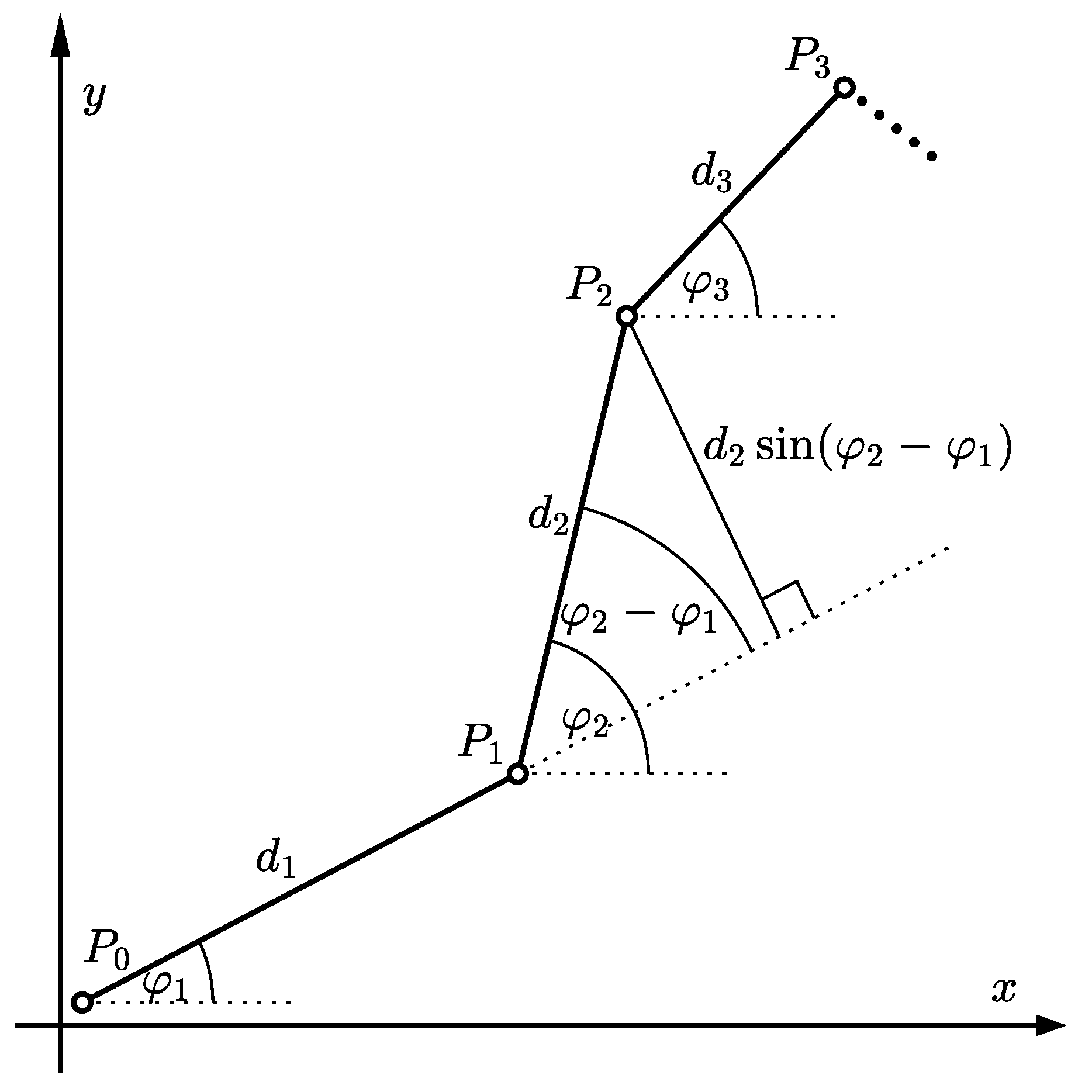
Bézier curves are parametric curves that are often used in scientific work and practical applications [30,31,32,33] due to their advantageous properties such as smoothness, simple definition and interpretation, easy computational burden, etc. Moreover, being parametric curves in the form of polynomials with simple derivatives has sparked their use in the area of mobile robotics and autonomous mobile systems [5,11,25,35,36,37,38,39].

2.1. Bézier Curves

A Bézier curve of the n-th order is defined as:

$${\mathbf{B}}_n\left(\lambda \right)={\sum }_{i=0}^n{\mathbf{P}}_i\left(\genfrac{}{}{0pt}{}{n}{i}\right){\lambda }^i{(1-\lambda )}^{n-i},\lambda \in [0,1],$$

(1)

where ${\mathbf{P}}_i$ are the vectors representing the so-called control points $P_i$ ($i=0,1,2,\dots n$) in the Euclidean coordinate system. In this work, only planar curves in the $(x,y)$ plane will be dealt with, so ${\mathbf{B}}_n\left(\lambda \right),{\mathbf{P}}_i(i=0,1,2,\dots n)\in {\mathbb{R}}^2$.

Bézier curves of a high order can meet a lot of constraints and could be used for describing a complex planar curve in the parametric form given by Equation (1). However, as it will be shown later, high-order curves also suffer from some problems. Typically, a large number of low-order curves are used instead to describe the planar curve. Such composite Bézier curves are composed of individual segments, each given by Equation (1).

Let us analyse some geometric properties of the Bézier curve given by Equation (1). The end points of the curve are $P_0$ and $P_n$:

$$\begin{array}{cc}\hfill \underset{\lambda \to 0}{lim}{\mathbf{B}}_n\left(\lambda \right)& ={\mathbf{P}}_0\hfill \\ \hfill \underset{\lambda \to 1}{lim}{\mathbf{B}}_n\left(\lambda \right)& ={\mathbf{P}}_n\hfill \end{array}$$

(2)

The orientations of the tangents at the endpoints of the Bézier curve can be obtained by finding the derivatives of the function ${\mathbf{B}}_n$ with respect to the independent variable $\lambda$ (at $\lambda \in \{0,1\}$):

$$\begin{array}{cc}\hfill \underset{\lambda \to 0}{lim}\frac{d}{d\lambda }{\mathbf{B}}_n\left(\lambda \right)& =n({\mathbf{P}}_1-{\mathbf{P}}_0)\hfill \\ \hfill \underset{\lambda \to 1}{lim}\frac{d}{d\lambda }{\mathbf{B}}_n\left(\lambda \right)& =n({\mathbf{P}}_n-{\mathbf{P}}_{n-1})\hfill \end{array}$$

(3)

Equations (2) and (3) reflect the symmetry of Bézier curves, i.e., the same curve (with opposite direction) is obtained if the sequence of the control points is reversed. This is why, all the properties that hold for the starting point also hold for the ending point. According to Equations (2) and (3), the starting point of the curve is given by the 0-th control point $P_0$, while the initial orientation coincides with the vector $\overrightarrow{P_0{P}_1}$.

2.2. The Curvature of Bézier Curves

The curvature of the path of the moving vehicle will play a key role in this paper. The curvature is inversely proportional to the radius of curvature. The curvature $\kappa$ at a certain point of the curve can have a positive value (the vehicle is turning in the positive direction, i.e., turning left), a negative value (turning right), or 0 (the vehicle is driving straight; this also happens at the point where the left curve joins the right one). The curvature of the path directly influences accelerations and jerks acting on the vehicle driving along the path. If we assume that the vehicle is driving along the path with velocity v (we also call this velocity tangential velocity), the acceleration in the tangential direction is $\dot{v}$ while there also exists the other component of the acceleration that is due to the curvature and acts in the direction perpendicular to the motion—this so-called radial acceleration is given by $v^2\kappa$. Sometimes, we are also interested in the third derivative of the position, the jerk. The tangential component of the jerk associated with the motion along the path is $(\ddot{v}-{\kappa }^2{v}^3)$, and the radial component is $\left(v^{-1}\frac{d}{dt}\left(v^3\kappa \right)\right)$. In order to keep the masses driving along the curved paths, the external forces are needed to produce appropriate accelerations. As shown above, these forces increase with increasing curvature. In order to keep these forces acceptable for driving comfort and to reduce mechanical wear, the curvature of the path should be low. Furthermore, variation of the curvature along the curve contributes to the radial jerk. In this work, we will treat curves or paths with the continuous curvature. An important consequence of the continuous-curvature path is that when driving with the continuous tangential acceleration $\dot{v}$, both the tangential and the radial jerk are bounded. If, however, the curvature is not continuous in some point, an infinite spike of the radial jerk cannot be avoided in this point, no matter how low the velocity and/or the acceleration are.

The curvature of the planar curve given in the parametric form is given as follows:

$$\kappa =\frac{x^{\prime }{y}^{″}-y^{\prime }{x}^{″}}{{\left({x^{\prime }}^2+{y^{\prime }}^2\right)}^{\frac{3}{2}}}$$

(4)

where primes indicate derivatives with respect to the independent variable $\lambda$. It is easy to see from (1) that in the case of Bézier curves $x\left(\lambda \right)$ and $y\left(\lambda \right)$ are polynomials of the n-th order while the order of their first and second derivatives are $(n-1)$ and $(n-2)$, respectively. The order of the each term of the numerator of (4) is therefore $(2n-3)$ but the highest powers of $\lambda$ cancel, and the order of the numerator of (4) is in general $(2n-4)$ (it is possible that for certain choice of control points the leading coefficient becomes 0).

Why is the order of the numerator of (4) important? Any polynomial of m-th order can have at most m real roots. The denominator of Equation (4) is positive except in a special case where all the control points coincide and the curve shrinks into a point. This means that the curvature given by Equation (4) can change the sign at most $(2n-4)$ times on the interval of interest $\lambda \in [0,1]$. Not only the curvature is important but also its derivative with respect to $\lambda$. It can easily be derived that the stationary points of the rate of change of the curvature coincide with the roots of the polynomial of degree $(4n-7)$. It is therefore possible to have up to $(4n-7)$ local minima and maxima of the curvature as a function of $\lambda$. We see that the number of oscillations increases rapidly with the polynomial order. This is a similar effect as the Runge’s phenomenon. For illustration purposes, a Bézier curve of the third order can have at most 2o zeros of the curvature and at most 5 zeros of its derivative (with respect to $\lambda$) while a Bézier curve of the fifth order can have at most 6 zeros of the curvature and at most 13 zeros of its derivative. This is a huge difference in the number of the zeros with a relatively small difference in the order, and consequently, to decrease oscillations of the curvature, the order of the polynomials involved should be kept as low as possible.

The curvature of the Bézier curve at the endpoints will be given as a function of the geometric properties of the control points. An arbitrary Bézier curve of an arbitrary order n is shown in Figure 1. After a short derivation we can obtain the expression for the curvature at the starting point:

$$\underset{\lambda \to 0}{lim}\kappa \left(\lambda \right)=\frac{n-1}{n}\frac{d_{2}sin({\phi }_2-{\phi }_1)}{{d_1}^2}$$

(5)

We see that the curvature at the endpoint depends only on the first (or last) three control points of the Bézier curve. An important consequence of Equation (5) is that the initial curvature of the Bézier curve will not change if the point $P_2$ is moved on a line parallel to the line through $P_0$ and $P_1$. This observation will be crucial for our choice of parameters.

From this point on we will limit our analysis to the case $n=3$. This means that there are four control points ($P_0$, $P_1$, $P_2$, $P_3$) that define the Bézier curve (as depicted in Figure 1). Following from Equation (5), the formulas for the initial and the final curvature are given by:

$$\begin{array}{cc}\hfill {\kappa }_0& =\underset{\lambda \to 0}{lim}\kappa \left(\lambda \right)=\frac{2}{3}\frac{d_{2}sin({\phi }_2-{\phi }_1)}{{d_1}^2}\hfill \\ \hfill {\kappa }_3& =\underset{\lambda \to 1}{lim}\kappa \left(\lambda \right)=\frac{2}{3}\frac{d_{2}sin({\phi }_3-{\phi }_2)}{{d_3}^2}\hfill \end{array}$$

(6)

2.3. Parametrization of Motion Primitives

We will parametrize the primitive given some geometric properties of the curve at its endpoints. The input parameters for the motion primitives will be:

• The position of both endpoints, i.e., $P_0$ and $P_3$;
• The orientation in both endpoints, i.e., angles ${\phi }_1$ and ${\phi }_3$; and
• The curvature in both endpoints, i.e., ${\kappa }_0$ and ${\kappa }_3$.

We will refer to the above information as the boundary conditions because they define the properties of the primitive at its endpoints or boundaries. Angles ${\phi }_1$ and ${\phi }_3$ can be interpreted as the initial and the final orientation, respectively. We will define two additional parameters analogous to $d_i$ and ${\phi }_i$ that apply to individual segments. Let D and $\varphi$ represent the Euclidean distance between $P_0$ and $P_3$, and the angle between the vector $\overrightarrow{P_0{P}_3}$ and the x axis, respectively. These two parameters can be computed easily given the endpoints $P_0$ and $P_3$. After a simple derivation, these two parameters can substitute $d_2$ and ${\phi }_2$ in the expressions for the curvature (6):

$$\begin{array}{cc}\hfill {\kappa }_0& =\frac{2}{3}\frac{Dsin\left(\varphi -{\phi }_1\right)-d_{3}sin\left({\phi }_3-{\phi }_1\right)}{{d_1}^2}\hfill \\ \hfill {\kappa }_3& =\frac{2}{3}\frac{Dsin\left({\phi }_3-\varphi \right)-d_{1}sin\left({\phi }_3-{\phi }_1\right)}{{d_3}^2}\hfill \end{array}$$

(7)

We will rewrite these two equations to obtain the final form that will be used for constructing the motion primitives in this paper:

$$\begin{array}{cc}\hfill \frac{3}{2}{\kappa }_0{d_1}^2+d_{3}sin\left({\phi }_3-{\phi }_1\right)& =Dsin\left(\varphi -{\phi }_1\right)\hfill \\ \hfill \frac{3}{2}{\kappa }_3{d_3}^2+d_{1}sin\left({\phi }_3-{\phi }_1\right)& =Dsin\left({\phi }_3-\varphi \right)\hfill \end{array}$$

(8)

Note that all the angles (${\phi }_1$, ${\phi }_3$, $\varphi$) can be given in all the possible directions from $-\pi$ to $+\pi$ (technically, all the equations also hold if the angles are outside of this interval). When inserting the boundary conditions, Equation (8) can be seen as a system of two quadratic equations with two unknowns ($d_1$ and $d_3$). Solving this system of equations for $d_1$ and $d_3$ gives all the control points and finally the explicit form of the primitive itself.

2.4. Reconstruction of the Motion Primitive from the Boundary Conditions

The system of equations presented by Equation (8) can best be depicted in a graphical form in the $(d_1,d_3)$ plane. In order to do so, we will rewrite Equation (8):

$$\begin{array}{cc}\hfill d_3& =\frac{Dsin\left(\varphi -{\phi }_1\right)}{sin\left({\phi }_3-{\phi }_1\right)}-\frac{3{\kappa }_0}{2sin\left({\phi }_3-{\phi }_1\right)}{d_1}^2=v_3-l_3{d}_1^2\hfill \\ \hfill d_1& =\frac{Dsin\left({\phi }_3-\varphi \right)}{sin\left({\phi }_3-{\phi }_1\right)}-\frac{3{\kappa }_3}{2sin\left({\phi }_3-{\phi }_1\right)}{d_3}^2=v_1-l_1{d}_3^2\hfill \end{array}$$

(9)

The equations in (9) represent two parabolas. The first one with the vertex $v_3$ on the $d_3$ axis opens either upward (U-type) if the leading coefficient $l_3$ is positive, or downward (D-type) if the leading coefficient $l_3$ is negative. The second parabola with the vertex $v_1$ on the $d_1$ axis opens either to the left (L-type) if the leading coefficient $l_1$ is negative, or to the right (R-type) if the leading coefficient $l_1$ is positive. When there is no curvature, the parabolas become straight lines, either horizontal (H-type) if $l_3=0$ or vertical (V-type) if $l_1=0$. All these types can further be classified into cases where the vertex of the parabola is positive (index +) or negative (index −). Note that $l_1$ and $l_3$ are of the same sign if and only if ${\kappa }_0$ and ${\kappa }_3$ are of the same sign.

It is important to note we are only interested in the positive solutions for $d_1$ and $d_3$ (negative solutions for $d_1$ and/or $d_3$ represent opposite orientations in the respective endpoint), so we will only focus on the first quadrant of the $(d_1,d_3)$ plane. In the first quadrant, only four type possibilities exist for the first parabola in (9), they are depicted with thick lines in Figure 2. There also exist four possible types for the second parabola—depicted with thin lines in Figure 2. So, the solution of the system of equations in Equation (8) is shown with the circle at the intersection of a thick and a thin line.

Two parabolas can have at most four intersections. If we limit ourselves only to the first quadrant, there cannot be more than three intersections. In order to analyse the number of solutions, we should note the following facts for the shape of the functions in the first quadrant:

• U-type and R-type functions are increasing while D-type and L-type are decreasing;
• Only U-type functions are convex while D-type, R-type, and L-type are concave.

Some important observations about the number of intersections of different functions:

• An increasing and a decreasing function can have at most one intersection;
• A decreasing convex function and a decreasing concave function can have at most two intersections (the same is true if both functions are increasing);
• Two decreasing concave functions (or any other of the three combinations decreasing-convex, increasing-concave, increasing-convex) can have more than two intersections.

So, the system of equations in Equation (8) can have the following number of distinct solutions satisfying $d_1>0,d_3>0$:

• One solution. This is the most frequent case that gives a unique Bézier curve.
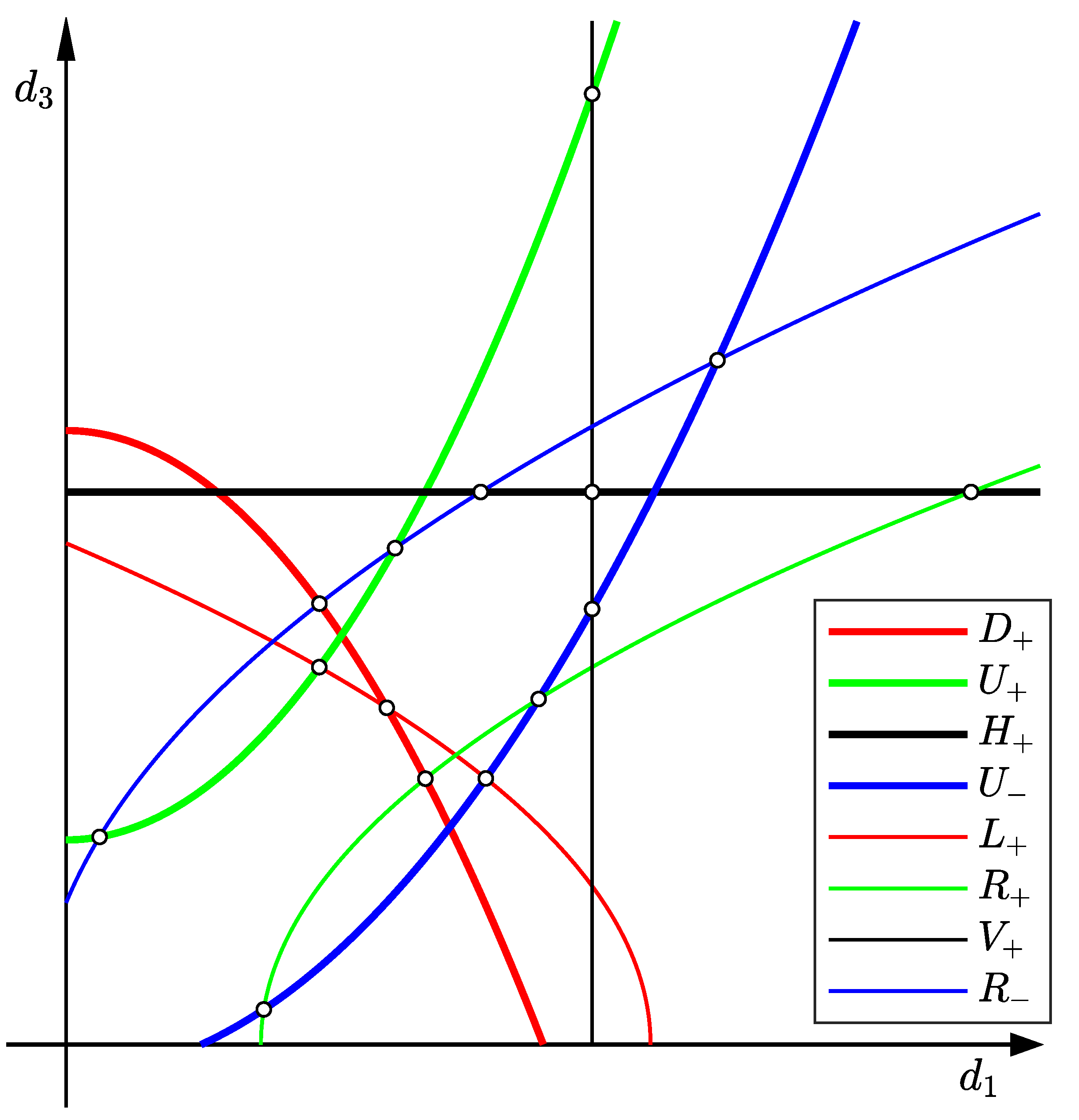
• Two solutions. This happen rarely because the boundary conditions given above are quite restricting. An example is given in Figure 2 (the intersection of a green and a blue line).
• Three solutions. This can only happen if one function is $D_{+}$ and the other is $L_{+}$ and the parameters of both parabolas are extremely restricted. Two intersections lie very close to both axes. The solutions with very low values of $d_1$ and/or $d_3$ often result in a high-curvature path near the endpoints and should be avoided.
• No solutions. This happens when the parabolas do not have intersections in quadrant 1. Examples in Figure 2: two green lines, a black line, and a red line. We have to also mention here the cases where the parabolas do not even enter quadrant 1—the vertex is negative and the leading coefficient $l_1$ (or $l_3$) is negative.

Remark 1.

If the system of equations in Equation (8) has no solutions, then no Bézier curve of the third order exists that meets all the boundary conditions. This happens when these conditions are demanding in the sense that the resulting curve would be unnatural for a simple motion primitive. In such cases, the curve should be split into two primitives which gives the designer additional degrees of freedom to construct the desired path. In Section 3.1, an algorithm will be given that produces a composite Bézier curve where the boundary conditions of the individual primitives are chosen so that the existence of the solution is guaranteed.

Remark 2.

If the system of equations in Equation (8) has more than one solution, there exist more (two or even three) distinct curves that all meet the given boundary conditions. An example is given in Figure 3 where bottom left and bottom right curves both meet the same boundary conditions although they are structurally quite different. Note that this example also relates to “demanding” conditions where we start with turning left although our goal is on our right-hand side, and we finish with turning left although our starting point is on the opposite side.

Remark 3.

Special case: $sin\left({\phi }_3-{\phi }_1\right)=0$. This means that the directions of the initial and the final orientation are parallel. In this case, the original system of equations in Equation (8) decomposes into two quadratic equations that can be solved easily. Both equations have a distinct positive solution if $sin\left(\varphi -{\phi }_1\right)$ and ${\kappa }_0$ are of the same sign, and $sin\left({\phi }_3-\varphi \right)$ and ${\kappa }_3$ are of the same sign. Again, if we study the cases that give no solutions carefully, we see that the requirements are unnatural for a simple primitive.

Remark 4.

Very special case: $sin\left({\phi }_3-{\phi }_1\right)=0$ and $sin\left(\varphi -{\phi }_1\right)=0$ (consequently $sin\left({\phi }_3-\varphi \right)=0$). The initial and the final orientation lie on the same line which means that the primitive is a line segment. The curvature of the line is 0, so the solution only exists if ${\kappa }_0$ and ${\kappa }_3$ are both 0. The system (8) has infinitely many solutions. Since the algorithm has to produce some result, one possibility is to choose: $d_1=d_3=\frac{D}{3}$.

2.5. Basic Motion Primitives

The most natural motion primitives include a straight line (discussed in Remark 4), a left curve and a right curve. A simple right (or left) curve will be denoted as a C-shaped primitive. Slightly more complex primitive that has a very natural shape is an S-shaped primitive. Another primitive that can be described by a third order Bézier curve is a loop. Some examples of the motion primitives are shown in Figure 3.

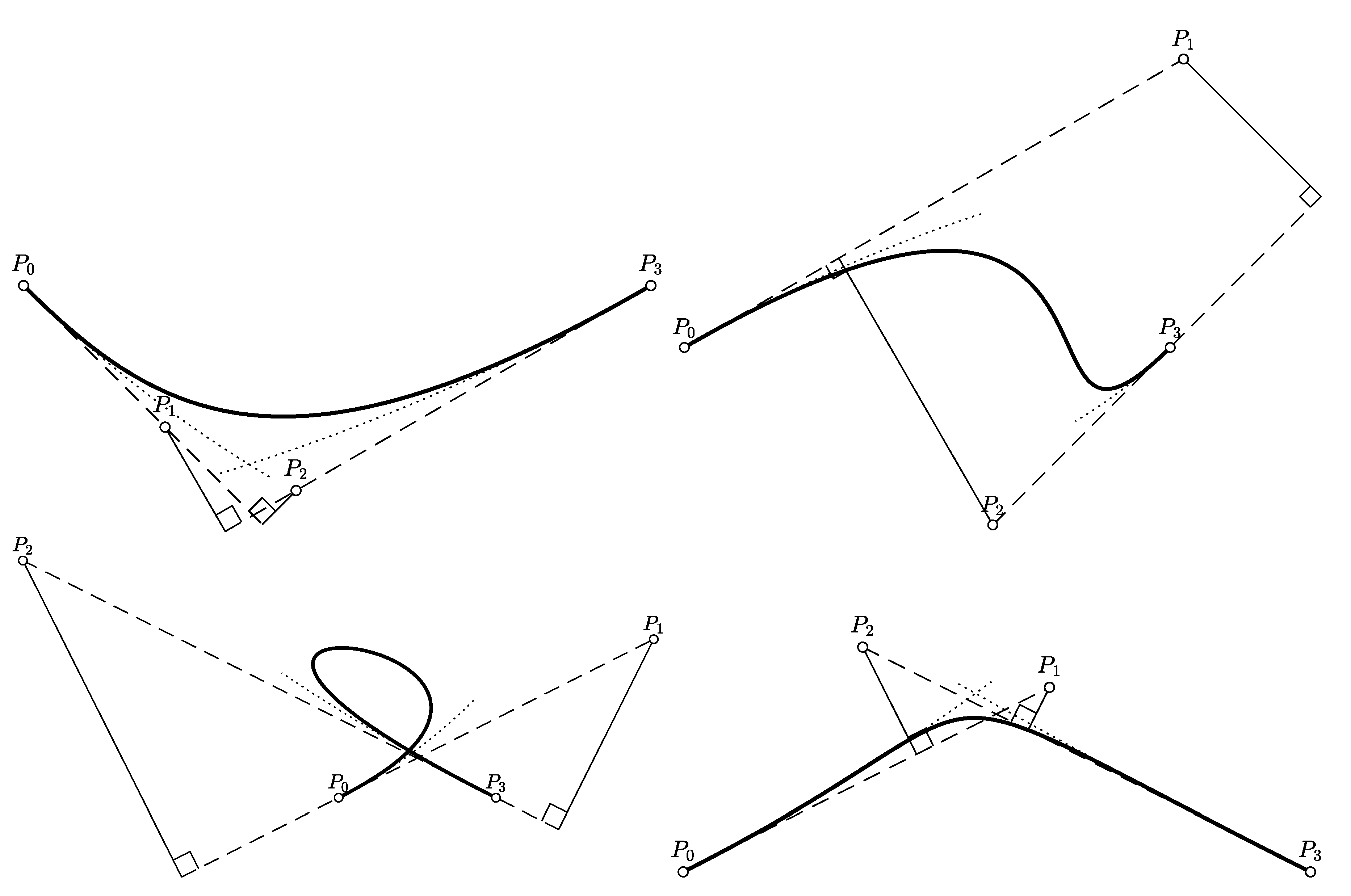
2.5.1. C-Shaped Primitive

A C-shaped curve (shown top left in Figure 3) is a simple left or right turn where the curvature does not change the sign throughout the curve. A C-shaped primitive is obtained if all the coefficients in the system of equations in Equation (8) have the same sign. In other words, $v_1$ and $v_3$ in Equation (9) are positive while $l_1$ and $l_3$ are negative. It is easy to see that we are dealing with a $D_{+}$ and an $L_{+}$ parabolas. Note that zero-curvature in either side also results in the C-shaped curve which means that the parabola collapses to a straight line ($V_{+}$ or $H_{+}$).

The intersection between two parabolas always exists as long as the curvatures are low enough. In the case where there is no intersection (one parabola lies above the other in the first quadrant), the intersection always appears by decreasing the curvature at one end or increasing it at the other. It is important to note that the solution is always obtained by changing just one curvature (initial or final). Furthermore, the solution can be obtained by changing just the requested one, not an arbitrary one. This will be important in the algorithm in Section 3.2 because we will only be allowed to change ${\kappa }_0$ while ${\kappa }_3$ will be fixed for each segment.

2.5.2. S-Shaped Primitive

An S-shaped primitive is a useful curve that consists of a left and a right curve (in any order) joined together in a single primitive. Such a curve (shown top right in Figure 3) has the curvature that changes its sign exactly once.

An S-shaped primitive is obtained if the curvatures ${\kappa }_0$ and ${\kappa }_3$ in Equation (8) are of a different sign. This means that the parabolas in (9) have the leading coefficients of the different sign. The possible combinations are either U-type and L-type or D-type and R-type. At least one of the vertices ($v_1$ and/or $v_3$) also has to be positive.

In Section 3.1, it will be shown how to choose the orientations in the intermediate points so that we always obtain the $L_{+}$ parabola. Now, we have two case for the other parabola:

• $U_{-}$ parabola. The intersection exists if the point of entry of the $U_{-}$ parabola into the first quadrant lies below the vertex of the $L_{+}$ parabola. If this is not the case, the intersection appears by increasing the curvature of the $U_{-}$ parabola. An alternative solution is to change the sign of the $L_{+}$ parabola which turns the primitive to the loop-shaped or V-shaped curve (shown in the bottom part of Figure 3).
• $U_{+}$ parabola. The intersection exists if the vertex of the $U_{+}$ parabola is lower than the point where parabola $L_{+}$ crosses from quadrant 1 to quadrant 2. It there is no intersection, one can be obtained by changing the curvature of the $U_{+}$ parabola. This then changes the primitive into C-shaped one.

2.5.3. Loop-Shaped Primitive and V-Shaped Primitive

A loop shaped primitive (shown bottom left in Figure 3) is a special type of a primitive that might be used in very specific circumstances. Similar path can be constructed by more primitives where the results can be supervised more easily. The curvature of the loop-shaped primitive does not change its sign. The control points of the loop-shaped primitive lie quite far from each other.

The V-shaped primitive (shown bottom right in Figure 3) slightly resembles letter V. It is distinguished from the C-shaped primitive by the fact that its curvature changes sign twice. In the beginning and the end the curvature is slightly positive (or negative) but in the middle a high-curvature curve of the different sign appears.

The V-shaped primitive is treated together with the loop-shaped one because they are two solutions of the same parametrization, i.e., the same boundary conditions. Both appear if the sign of the curvatures at the endpoints are the same (but opposite than in the case of C-shaped primitives). This results in an U-type parabola and an R-type one that have two intersections (an example of the intersections is given in Figure 2 with the a green and a blue line). The solution with higher values of $d_1$ and $d_3$ results in a loop, and the other results in a V-shaped curve.

3. Construction of the Path from Motion Primitives

In Section 2, we have shown how motion primitives can be obtained from the boundary conditions. In this section we will propose a solution for constructing an appropriate path for wheeled vehicles by joining together several motion primitives. Technically, the path is defined as a planar curve with given initial and final pose (position and orientation). The curve should satisfy $C^2$ continuity. The curve will be composed of several third-order Bézier primitives. In order to apply Algorithm 1 proposed in Section 2 for constructing the path, the following information has to be predefined:

• Waypoints or intermediate points denoted by the sequence $W_0,W_1,\dots W_N$ ($W_0$ and $W_N$ are the initial and the final position, respectively);
• The orientation in the waypoints denoted by the sequence ${\theta }_0,{\theta }_1,\dots {\theta }_N$ (${\theta }_0$ and ${\theta }_N$ are the initial and the final orientation, respectively);
• The curvature in the intermediate points denoted by the sequence $K_0,K_1,\dots K_N$.

Algorithm 1: The algorithm for calculation of motion primitives from boundary conditions.

In general, the solution of the system of equations in Equation (8)—or the intersection of parabolas in (9)—is obtained by following these steps: Introduce $d_3$ given by the first equation in (9) into the second equation in (9) which results in a depressed quartic (the polynomial of the fourth order without the cubic term). Find the roots of the quartic polynomial. Remove complex and negative solutions among the four solutions which results in $d_1$. (The cases with more or no solutions are discussed in Remarks 1 and 2). Calculate $d_3$ from $d_1$ using the first equation in (9). Calculate control points $P_1$ and $P_2$. Apply the formula in Equation (1) to obtain the parametric form of the motion primitive.

The path is then constructed by treating each segment separately. On each segment all the necessary information is readily available to describe the problem as given by the system of quadratic equations in Equation (8). The system is then solved by finding the intersections of the parabolas representing the equations as shown in Section 2. After resolving all the segments of the path, the whole path that satisfy all the boundary conditions is completely known and given in the parametric form. Let us emphasize again that the resulting path composed of individual primitives is infinitely differentiable except in the intermediate points where the path and the first two derivatives are continuous ($C^2$ continuity).

The above mentioned approach is problematic if all the necessary information is not available. It is quite safe to assume that the waypoints are known. When the designer faces the problem of path planning, he or she needs to know the points that the path will cross. They are either explicitly known, prespecified by the design requirements, given as a result of a certain path-planning algorithm, determined graphically by some kind of interpolation or other method, or even given by an optimization algorithm that minimizes certain criterion of the path. On the other hand, the information about the orientation and/or the curvature in the intermediate points might not always be readily available. It would therefore be very useful to have some guidelines how to choose it. We will next propose a method that gives the orientation in the waypoints. This not only simplifies the approach but also guarantees that Algorithm 1 always gives a unique solution.

3.1. The Algorithm for Proposing Suitable Orientations in Waypoints

We will assume here that the waypoints are known and the orientations in the initial and the final points are given (denoted by ${\theta }_0$ and ${\theta }_N$) while the proposed algorithm gives the orientations in the waypoints. The algorithm runs from the end of the curve towards the start and determines the orientations in the waypoints:

$${\theta }_i={\varphi }_i-f({\theta }_{i+1}-{\varphi }_i),i=N-1,N-2,\dots 1$$

(10)

where ${\varphi }_i$ is the angle between the vector $\overrightarrow{W_i{W}_{i+1}}$ and the positive direction of the x axis, and f is a design parameter that will be discussed later. In simple words, ${\varphi }_i$ are the angles of the lines through the endpoints of the individual segments. Note that ${\theta }_i$, ${\theta }_{i+1}$, and ${\varphi }_i$ correspond to ${\phi }_1$, ${\phi }_3$, and $\varphi$ in Equation (8). For the analysis of solutions of (8), the following corollaries of (10) can easily be derived:

$$\begin{array}{cc}\hfill {\varphi }_i-{\theta }_i& =f({\theta }_{i+1}-{\varphi }_i),i=N-1,N-2,\dots 1\hfill \\ \hfill {\varphi }_i-{\theta }_i& =\frac{f}{1+f}({\theta }_{i+1}-{\theta }_i),i=N-1,N-2,\dots 1\hfill \\ \hfill {\theta }_{i+1}-{\varphi }_i& =\frac{1}{1+f}({\theta }_{i+1}-{\theta }_i),i=N-1,N-2,\dots 1\hfill \end{array}$$

(11)

Parameter f will be chosen on the interval $(-1,1)$ which results in the expressions $({\theta }_{i+1}-{\varphi }_i)$ and $({\theta }_{i+1}-{\theta }_i)$ being of the same sign which follows from the third equation in (11). Consequently, the vertex $v_1$ of the second parabola in (9) is always positive. The sign of f will be based on the type of the primitive selected by the designer (S or C).

Based on the analysis given in Section 2.5.1, C-shaped primitive is obtained when the curvatures at the endpoints are of the same sign and the intermediate orientations are suggested by (10) with $f>0$. A typical value that gives good results is $f=0.2$. This suggestion has a plausible explanation: When we face the end of the segment from its beginning and the final orientation appears to the left (right) from this viewpoint, the initial orientation should be obtained by turning slightly to the right (left). Then, the path is obtained by a single left (right) curve.

Based on the analysis given in Section 2.5.2, S-shaped primitive could be obtained when using the intermediate orientations suggested by (10) with positive or negative sign (only $-1<f<0$). Typical value that give good results are $f=\pm 0.2$. Choosing negative f (larger than $-1$) results in the parabolas of the $U_{-}$ and $L_{+}$ type in Equation (9) while positive f results in the parabolas of the $U_{+}$ and $L_{+}$ type.

3.2. The Algorithm for Proposing Suitable Curvatures in Waypoints

The algorithm will determine curvatures in the waypoints so all the segments will have a unique solution of the motion primitive. The last segment is treated first. If the orientations are chosen using (10) with $f>-1$, the second parabola in Equation (9) always has a positive vertex. Now the curvature in the final point $W_N$ (it will be denoted by $K_N$) is selected so that the second parabola will be of the $L_{+}$ type. An appropriate way of choosing the curvature is to force the parabola to leave the first quadrant at $d_3=\frac{D}{2}$. Apart from the unknowns ($d_1$ and $d_3$), all the parameters in Equation (9) are already known at this point except ${\kappa }_0$. We have already determined that the second equation corresponds to the $L_{+}$ type parabola because of (10). The first equation in (8) corresponds to the parabola with ${\kappa }_0$ to be determined. There is plenty of freedom to choose the curvature ${\kappa }_0$ so that the parabolas intersect. One thing to note here is that in most cases the distance between the first two control points of the Bézier curve ($d_1$) should be similar to the distance between the last two control points ($d_3$). Based on this observation, we will propose the following relation:

$$d_3=g{d}_1$$

(12)

where g is a design parameter to choose. Usually it is chosen around 1. Now we can obtain $d_1$ and $d_3$ following the next steps:

• Obtain the intersection of the parabola given by the second equation in (9) and a straight line given by (12). The intersection always exists in the first quadrant because the parabola is of $L_{+}$ type.
• $d_3$ follows directly from (12).
• The curvature ${\kappa }_0$ is obtained from the first equation in (9). (We could also analyse the first parabola in (9). If the intersection is above the vertex, the curve is C-shaped. If the intersection is below the vertex, the curve is S-shaped.)

The algorithm then proceeds with the previous segment, and we continue until we finish the first one.

4. Examples and Comparisons

In this Section two practical examples of using the proposed algorithms will be treated.

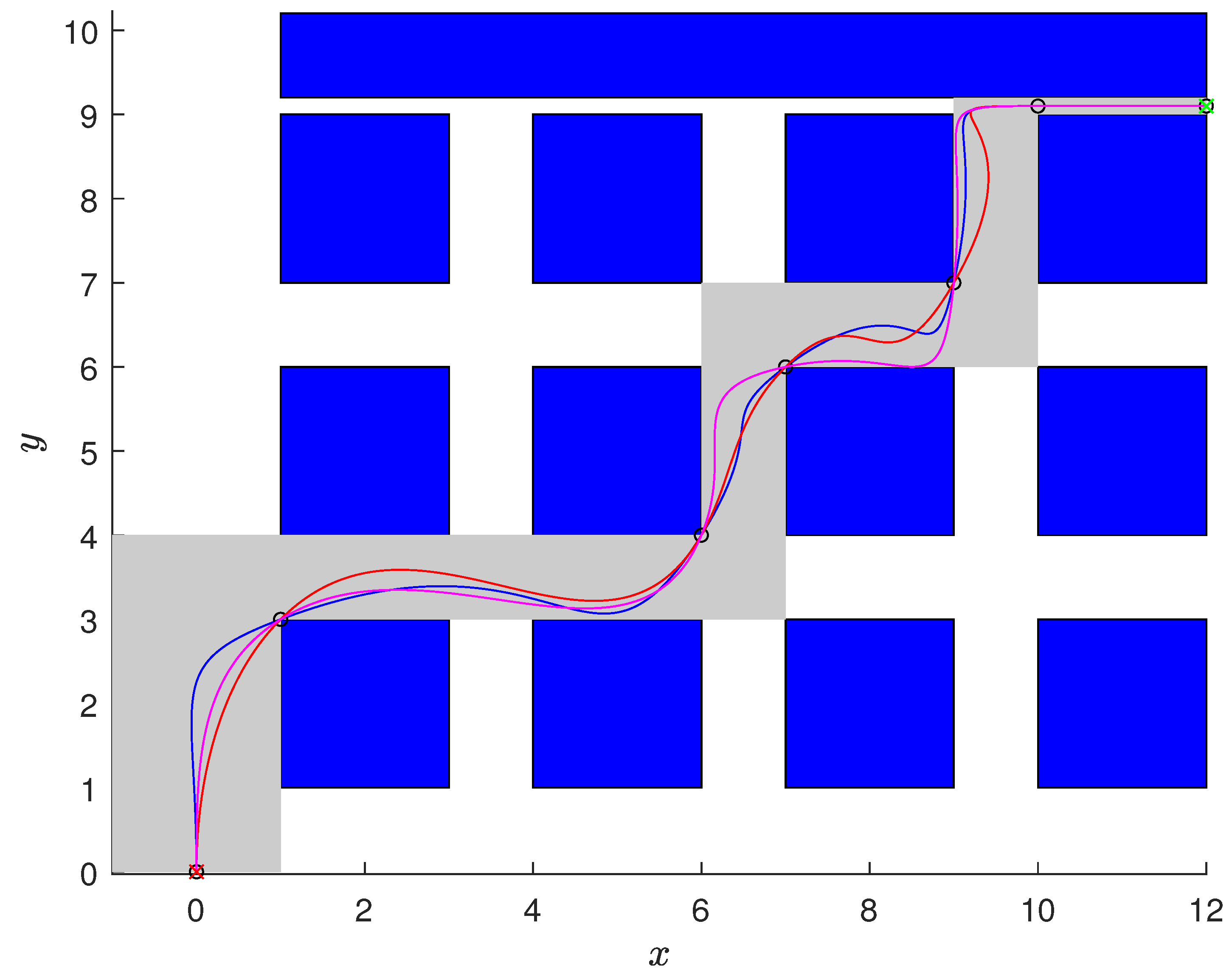
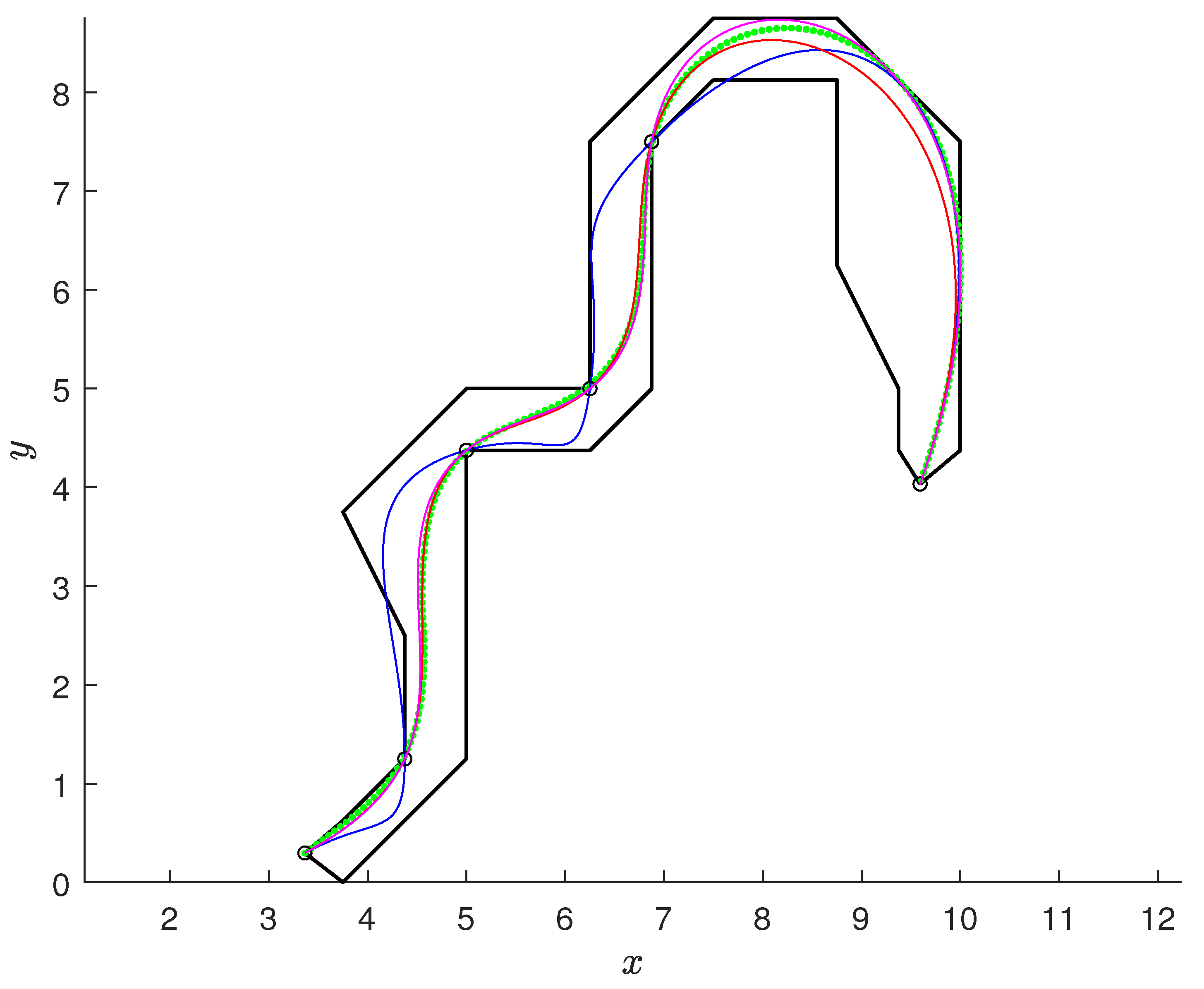
4.1. Example 1: A Path in a Given Corridor

We will now test the proposed approach on a simple example. A layout depicted in Figure 4 is assumed. Blue patches represents the forbidden area while grey corridor that should contain the path is chosen taking into account some criterion. Note that we do not take into account the size of the robot or any practical limitations. In this example we simply search for the path to be contained in a specific area. The goal is to find a continuous-curvature path that starts in the red cross and finishes in the green cross. First, we need to identify waypoints. We could use some algorithm but in this case waypoints are obvious and are given by black circles in Figure 4. Note that there are also some additional limitations: the initial orientation is ${90}^{\circ }$, the final orientation is $0^{\circ }$, and the curvature on the last segment is 0. We will apply Algorithm 1 to find the path on the first five segments. In the first try, we will choose the orientations and curvatures based on the fact we know our waypoints and we roughly know where to make turns. The orientations in the seven waypoints (including the initial and the final) have been chosen as: ${90}^{\circ }$, ${45}^{\circ }$, ${60}^{\circ }$, ${45}^{\circ }$, ${60}^{\circ }$, $0^{\circ }$, $0^{\circ }$. The curvatures have been chosen as: 0, $-0.4$, $0.4$, $-0.4$, $0.2$, 0, 0. The resulting path is shown in Figure 4 and the curvature in Figure 5 (both with red colour). Note that the independent variable of each segment is $\lambda$ that runs from 0 to 1 in Bézier curves, but here $\lambda$ runs from one integer to the next one during one segment. The second path was obtained by applying the algorithm for suggesting orientations ($f=0.2$ was chosen for the C-shaped segments—the first and the last—and $f=-0.2$ for the S-shaped ones—the second, the third, the fourth)—and curvatures (the design parameter g was chosen as $g=0.7$). The results are depicted with blue colour in Figure 4 and Figure 5. In the last part of this experiment, the free orientations and curvatures were searched for by optimization where the cost function consisted of the part that minimizes the integral of ${\kappa }^2\left(\lambda \right)$ on $\lambda \in [0,6]$, and the second part was added to penalize the curves that leave the corridor. The resulting path is depicted with magenta colour in Figure 4 and Figure 5.

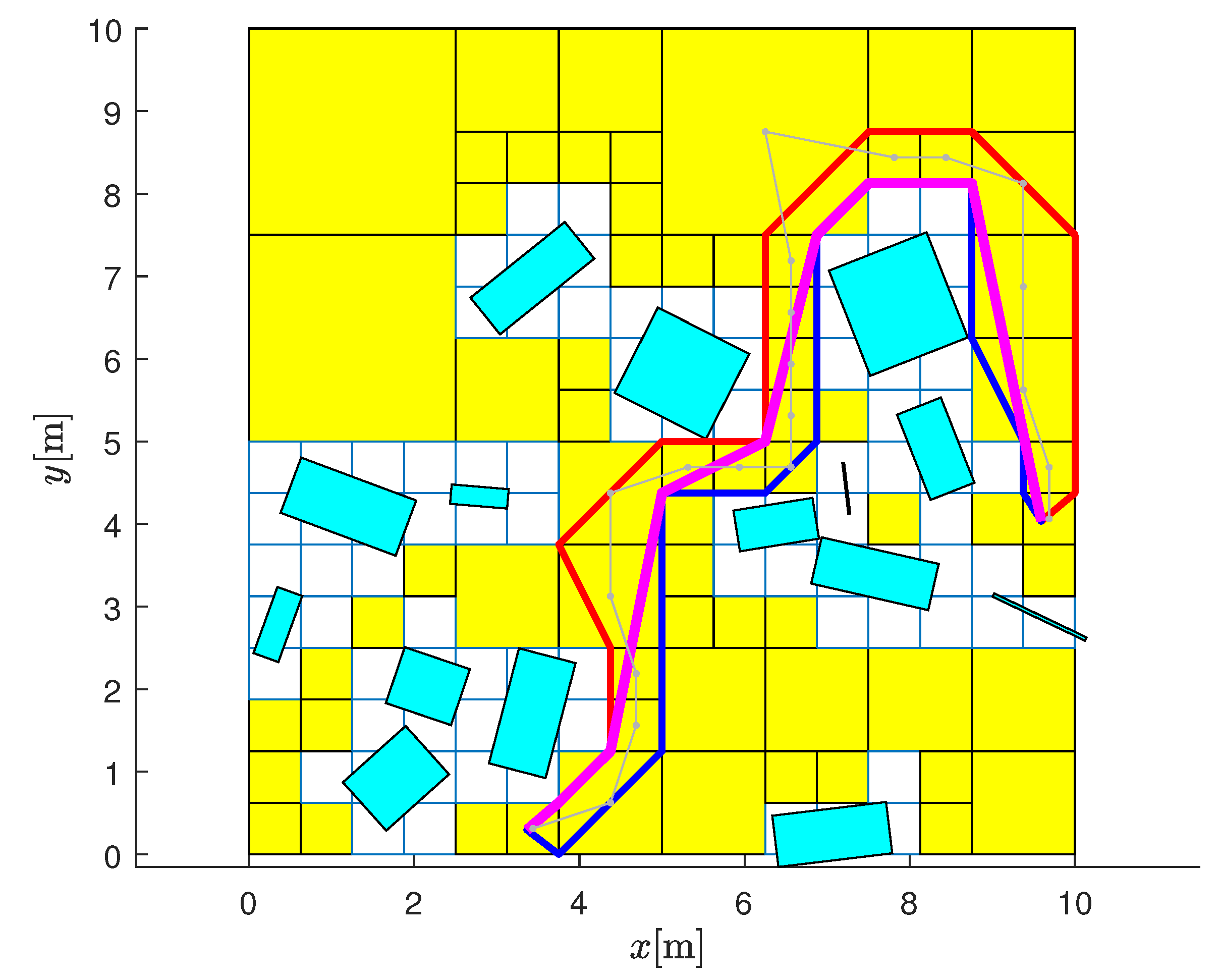
4.2. Example 2: Environment with Random Obstacles—Comparison with an Existing Method

The proposed primitives can also be applied in environments with obstacles to define smooth paths with continuous curvature.

The initial information for the path calculation is provided by a safe corridor and an optimised path consisting of straight-line segments within the corridor (see Figure 6). The environment is first decomposed into square cells using the Quadtree decomposition. The optimal path from the cell with the start position to the cell with the goal position is determined using the A${}^{*}$ algorithm. The A${}^{*}$ path connects the centres of free cells, where the neighbourhood of the cells is defined by cells that have a common edge. The cells along the optimal path define the corridor within which the optimised path is calculated using the funnel algorithm [40].

The capabilities of the proposed motion planner in path planning applications are also illustrated by comparisons. The proposed motion planner solution is compared with an optimisation-based path planner on a race track proposed in [41]. The approach performs a comprehensive optimisation of the path within a given corridor (e.g., corridor in Figure 6) to find the path shape that minimises the overall curvature of the solution. A brief summary of the approach is as follows. The discrete kinematics of the vehicle is defined by

$$\begin{array}{c}x(i+1)=x\left(i\right)+\mathsf{\Delta }s\left(i\right)cos\left(\theta \left(i\right)+\frac{\mathsf{\Delta }s\left(i\right)\kappa \left(i\right)}{2}\right)\hfill \\ y(i+1)=y\left(i\right)+\mathsf{\Delta }s\left(i\right)sin\left(\theta \left(i\right)+\frac{\mathsf{\Delta }s\left(i\right)\kappa \left(i\right)}{2}\right)\hfill \\ \theta (i+1)=\theta \left(i\right)+s\left(i\right)\kappa \left(i\right),\hfill \end{array}$$

(13)

where $x\left(i\right)$, $y\left(i\right)$, $\theta \left(i\right)$ define the pose of the vehicle at the i-th point along the path. The control variables are the current curvature of the vehicle $\kappa \left(i\right)$ and the driving distance $\mathsf{\Delta }s\left(i\right)$ between adjacent points. Assuming that $\mathsf{\Delta }s\left(i\right)=\mathsf{\Delta }s$ is constant and predefined, the vehicle path is defined by the initial vehicle pose and the progression of $\kappa \left(i\right)$ along the path. We have searched for the optimal path within the given corridor (e.g., in Figure 6) using constrained optimisation, which minimises the objective function J at the current point i taking into account the prediction for h future points

$$\begin{array}{cc}\hfill J\left(i\right)& =\underset{\kappa \left(j\right)}{min}\sum _{j=i}^{i+h}{\kappa }^2\left(j\right)\hfill \\ \\ \hfill & \mathrm{subject} \mathrm{to}: \mathrm{stay} \mathrm{inside} \mathrm{provided} \mathrm{corridor}.\hfill \end{array}$$

(14)

Once the optimal parameters $\kappa \left(j\right)$ for the prediction horizon $j\in i,\cdots ,i+h$ are found, the first one ($\kappa \left(i\right)$) is used to move to the next vehicle pose $(i+1)$ using kinematics (13). The algorithm then continuous in a classical receding horizon fashion. Thus, the optimisation searches for the path within a corridor that has a minimum curvature in the prediction horizon h. Since the local curvature defines the maximum permissible vehicle speed to prevent lateral sleep the path optimised according to the criteria J in (14) is a good estimate for the fastest possible path within the corridor [41].

In the following optimisations, we set the horizon h to the half of the total path length. In Figure 6, the estimated path length in the corridor is $L=15$ and is described by $N=200$ points, therefore the horizon includes $h=100$ points and $\mathsf{\Delta }s=\frac{L}{N}$. The optimisation (14) is computationally intensive as it involves a large number of parameters (e.g., curvatures in a hundred points) and is performed at every point along the path.

The results of the described approach are depicted with green colour in Figure 7 and Figure 8. Green dots in Figure 7 show the points where the curvature was recalculated by optimization. Now, we will compare these results with the proposed algorithm. First, the waypoints have been identified. They are chosen as black circles in Figure 7. Note that relatively low number of segments have been used. The orientation in the waypoints has been determined by the algorithm in Section 3.1 where $f=0.2$ was chosen. Note that two orientations that were outside of the corridor were manually fixed to be on the boundary of the corridor. In the second step the algorithm in Section 3.2 was used to determine the curvatures ($g=1$ was used). The resulting path is shown in Figure 7 and its curvature in Figure 8 (both with blue colour). In Figure 7 and Figure 8 magenta colour is used for showing the results of the paths obtained by optimization minimizing the criterion:

$$I=\frac{{\int }_{s_0}^{s_L}{\kappa }^2\left(s\right)ds}{{\int }_{s_0}^{s_L}ds}$$

(15)

where s is the curve length ($s_0$ at the beginning and $s_L$ at the end of the curve). The criterion I from (15) gives average value of the squared curvature. The red colour in Figure 7 and Figure 8 shows the result of Algorithm 1 where the orientations and curvatures are “copied” from the green line. This means that only the results of the funnel algorithm in the waypoints are taken into account. Orientations and curvatures in the waypoints are then used as an input to Algorithm 1. It turns out that the shape of the whole path lies very close to the one obtained by the funnel algorithm but its curvature is much smoother. This suggests that the proposed approach could be used for smoothing paths obtained by some other algorithms.

Some statistics are shown in

Table 1. Four properties of the paths obtained by four different path-construction methods in Example 2.

Algorithm	Length	Average ${\mathit{\kappa }}^2$	Max $\mathit{\kappa }$	Min $\mathit{\kappa }$
funnel alg [40]	16.1395	0.2415	0.8669	$-1.0000$
Section 3.1 and Section 3.2	16.6174	0.6825	5.3447	$-1.2397$
optimization	16.3910	0.2451	0.8394	$-0.8666$
“filtering” of [40]	15.9238	0.2576	0.8493	$-1.0266$

. The first row shows the results of the funnel algorithm [40] (green colour in Figure 7 and Figure 8); the second row shows the results of Algorithm 1 with the orientations and curvatures proposed in Section 3.1 and Section 3.2 (blue colour in Figure 7 and Figure 8); the third row shows the results of Algorithm 1 with the orientations and curvatures proposed by the optimization (magenta colour in Figure 7 and Figure 8); the fourth row shows the results of Algorithm 1 with the orientations and curvatures “copied” from the funnel algorithm (red colour in Figure 7 and Figure 8). The first column shows the length of the path, the second shows the value of the cost function I from (15), the last two show the maximal and minimal values of the curvature.

The results presented in Figure 7 and Figure 8 and in Table 1 show that the basic algorithm that does not involve optimization produces satisfactory results but cannot compete with the results obtained by comprehensive optimizations. The funnel algorithm is able to obtain the lowest value of the cost function I from (15) which is understandable because it has the highest number of degrees of freedom. However, the other properties are not so good in comparison to the solutions obtained from Algorithm 1. Optimization-based results show low averages and low extrema of the curvature. The curvature also exhibits very smooth shape. It is worth mentioning that the approach where we copied the values of the curvature and the orientation in four waypoints also produces excellent results which shows that the third order Bézier curve with the proposed boundary conditions is able to “filter” the curve in a very natural way.

5. Discussion

Obtaining splines from multiple motion primitives is much less restrictive and more natural when using the geometric $C^2$ continuity of the combined path than when using the parametric $C^2$ continuity. A combined path using geometric continuity only needs to have the same tangent orientation and curvature in the joints, while parametric continuity requires the same derivatives of the path (e.g., the time derivatives such as velocities and accelerations). For this reason, the proposed approach only requires a third order Bézier curve compared to common approaches in the literature where higher order Bézier curves are required to ensure parametric continuity [5,11,25,35,36,37,38,39].

Lower order motion primitives are also advantageous because they have fewer possible oscillations between the endpoints where the boundary conditions are satisfied. Higher order Bézier curves are known to have poor numerical stability [18]. The disadvantage of using lower order splines is less freedom in curve shaping between endpoints. Therefore, more primitives must be combined to approximate the desired arbitrary path. So, instead of a higher order motion primitive with several free shape parameters, a spline is combined from several lower order primitives, where the shape parameters (also) become the intermediate joint points. Additionally, discontinuity of higher order derivatives may appear. More precisely, if the obtained path is driven by the continuous tangential acceleration, the resulting radial jerk is discontinuous but bounded in the joints (see Section 2.2) while higher derivatives such as snap can be unbounded.

Once you have determined the desired path according to the requirements of the environment and the application, e.g., collision-proof, shortest, or safest, this path must eventually be followed by a vehicle. This means that velocity profile must also be defined for this path according to the dynamic constraints of the vehicle (maximum speed and acceleration). Therefore, for trajectories where a velocity profile is also defined for a given path, splines of motion primitives are required that have parametric continuity. Furthermore, it is very helpful if the derivatives of these functions could be obtained analytically as is the case with the proposed approach. Thus, the problems of numerical differentiation are avoided.

We provide an analytical solution to obtain a motion primitive that can satisfy the required boundary conditions for position, orientation and curvature in the endpoints. Depending on the requirements, up to three different solutions can be found to satisfy the endpoint requirements. The most common case is that we have a single solution that results in a unique curve. Three solutions only exist in extremely rare cases and only one of them is meaningful. Two solutions (a loop-shaped primitive and a V-shaped one) occur when the boundary conditions are demanding and a simple curve that satisfy them does not exist. No solutions exist if the conditions are very difficult and unnatural for a simple curve. We could say that the cases with more or no solutions remind us that the boundary conditions are not chosen cleverly. In such cases, additional waypoints should be chosen to add more flexibility.

Normally, path planning algorithms specify waypoints that the mobile system must traverse on its way to the goal. Finally, the realised path connecting these points must be feasible for a wheeled vehicle, i.e., it must typically have continuous orientation and curvature. Besides the position of the waypoints which is usually available, we provide an algorithm that suggests suitable orientation and curvature which are usually not known. This algorithm selects the appropriate primitive type C-shaped or S-shaped and proposes the constraints that guarantee the solution of the composite path from the proposed third-order Bézier primitives. This solution may already be good enough for non-demanding applications (e.g., in free space or when no obstacles are crossed). For additional path requirements, such as minimum distance, minimum time, collision safety and or consideration of vehicle constraints on curvature, additional optimisation can be applied. In doing so, the proposed constraints can provide good initial conditions for the optimisation.

In the examples provided, both paths with the proposed initial boundary conditions in the waypoints and the optimised path according to the corridor requirements and the path comfort criteria [41] are shown. Both solutions are also compared with the path obtained with a complex optimisation where the vehicle kinematics and the optimised curvature are searched for a prediction horizon. The proposed solutions are quite close to the compared complex optimisation, indicating that the proposed primitives are natural and good candidates for path planning applications. The advantages of the optimised path obtained using the proposed primitive are the following. Compact analytic solution of the path, which has a nice and smooth (in joints of the primitives is $C^2$) course of curvature. On the other hand, a complex optimisation within the horizon can provide a better path according to the optimisation criteria, but it is more difficult to obtain a smooth course of curvature due to the complexity of the optimisation (high number of parameters, chattering effects between successive optimisations in the time instants, etc.). Therefore, the proposed solution with third-order primitives can also be used to smooth paths of some other existing solutions. No optimisation is required for the smoothing. Waypoints are simply selected along the existing solution (to obtain boundary conditions for the primitives) and the primitives are fitted to them, as also shown in the results.

6. Conclusions

A new parametrisation of low-order (third order) Bézier motion primitives with continuous curvature (i.e., $C^2$ geometric curve continuity) in joints is proposed. The primitive is obtained analytically where the solution satisfies the required boundary conditions for the position, orientation and curvature at the endpoints. Besides $C^2$ continuity and analytic solution, the proposed primitive has several other advantages resulting from its low order such as computational efficiency, minimal unwanted curve oscillations which typically appear at higher-order curves and better convergence when applied to planning optimizers. Practical instructions for constructing primitives and an effective algorithm that connects given waypoints with the primitives resulting in $C^2$ path are provided. Examples and comparisons confirm the applicability of the proposed motion primitives in path planning applications.

In the future, we will apply and validate the proposed primitives in practical applications, e.g., in a path optimizer for minimal-time safe path planning in a warehouse under variable load.

References

1. Montemerlo, M.; Becker, J.; Bhat, S.; Dahlkamp, H.; Dolgov, D.; Ettinger, S.; Haehnel, D.; Hilden, T.; Hoffmann, G.; Huhnke, B.; et al. Junior: The Stanford entry in the Urban Challenge. J. Field Robot. 2008, 25, 569–597. [Google Scholar] [CrossRef] [Green Version]
2. Likhachev, M.; Ferguson, D. Planning Long Dynamically-Feasible Maneuvers for Autonomous Vehicles. Int. J. Robot. Res. 2009, 28, 933–945. [Google Scholar] [CrossRef] [Green Version]
3. Choset, H.; Lynch, K.; Hutchinson, S.; Kantor, G.; Burgard, W.; Kavraki, L.; Thrun, S. Principles of Robot Motion: Theory, Algorithms, and Implementations; MIT Press: Cambridge, MA, USA, 2005; p. 603. [Google Scholar]
4. Webb, D.J.; van den Berg, J. Kinodynamic RRT*: Asymptotically optimal motion planning for robots with linear dynamics. In Proceedings of the 2013 IEEE International Conference on Robotics and Automation (ICRA), Karlsruhe, Germany, 6–10 May 2013; pp. 5054–5061. [Google Scholar]
5. Klančar, G.; Seder, M.; Blažič, S.; Škrjanc, I.; Petrović, I. Drivable Path Planning Using Hybrid Search Algorithm Based on E* and Bernstein–Bézier Motion Primitives. IEEE Trans. Syst. Man Cybern. Syst. 2021, 51, 4868–4882. [Google Scholar] [CrossRef]
6. Zhang, Q.; Song, Y.; Jiao, P.; Hu, Y. A Hybrid and Hierarchical Approach for Spatial Exploration in Dynamic Environments. Electronics 2022, 11, 574. [Google Scholar] [CrossRef]
7. Pozna, C.; Precup, R.E.; Földesi, P. A novel pose estimation algorithm for robotic navigation. Robot. Auton. Syst. 2015, 63, 10–21. [Google Scholar] [CrossRef]
8. Sánchez-Ibáñez, J.R.; Pérez-del Pulgar, C.J.; García-Cerezo, A. Path Planning for Autonomous Mobile Robots: A Review. Sensors 2021, 21, 7898. [Google Scholar] [CrossRef]
9. Vaščák, J.; Hvizdoš, J. Vehicle navigation by fuzzy cognitive maps using sonar and RFID technologies. In Proceedings of the 14th IEEE International Symposium on Applied Machine Intelligence and Informatics, Herlany, Slovakia, 21–23 January 2016; pp. 75–80. [Google Scholar]
10. Klančar, G.; Seder, M. Coordinated Multi-Robotic Vehicles Navigation and Control in Shop Floor Automation. Sensors 2022, 22, 1455. [Google Scholar] [CrossRef]
11. Neto, A.A.; Macharet, D.G.; Campos, M.F.M. Feasible RRT-based path planning using seventh order Bézier curves. In Proceedings of the 2010 IEEE/RSJ International Conference on Intelligent Robots and Systems, Taipei, Taiwan, 18–22 October 2010; pp. 1445–1450. [Google Scholar] [CrossRef]
12. Wang, H.; Li, G.; Hou, J.; Chen, L.; Hu, N. A Path Planning Method for Underground Intelligent Vehicles Based on an Improved RRT* Algorithm. Electronics 2022, 11, 294. [Google Scholar] [CrossRef]
13. Zhang, T.; Mo, H. Reinforcement learning for robot research: A comprehensive review and open issues. Int. J. Adv. Robot. Syst. 2021, 18, 17298814211007305. [Google Scholar] [CrossRef]
14. Choi, J.W.; Curry, R.; Elkaim, G. Piecewise Bezier Curves Path Planning with Continuous Curvature Constraint for Autonomous Driving. In Machine Learning and Systems Engineering; Lecture Notes in Electrical Engineering 68; Springer Science + Business Media: Berlin/Heidelberg, Germany, 2010; pp. 31–45. [Google Scholar]
15. Ghilardelli, F.; Gabriele, L.; Piazzi, A. Path Generation Using η4-Splines for a Truck and Trailer Vehicle. IEEE Trans. Autom. Sci. Eng. 2014, 11, 187–203. [Google Scholar] [CrossRef]
16. Velenis, E.; Tsiotras, P. Minimum-Time Travel for a Vehicle with Acceleration Limits: Theoretical Analysis and Receding-Horizon Implementation. J. Optim. Theory Appl. 2008, 138, 275–296. [Google Scholar] [CrossRef]
17. Chen, C.; He, Y.; Bu, C.; Han, J.; Zhang, X. Quartic Bezier Curve based Trajectory Generation for Autonomous Vehicles with Curvature and Velocity Constraints. In Proceedings of the IEEE International Conference on Robotics and Automation (ICRA), Hong Kong, China, 31 May–7 June 2014; pp. 6108–6113. [Google Scholar]
18. Zdešar, A.; Škrjanc, I. Optimum Velocity Profile of Multiple Bernstein-BéZier Curves Subject to Constraints for Mobile Robots. ACM Trans. Intell. Syst. Technol. 2018, 9, 1–23. [Google Scholar] [CrossRef]
19. Klančar, G.; Zdešar, A.; Blažič, S.; Škrjanc, I. Wheeled Mobile Robotics—From Fundamentals towards Autonomous Systems; Butterworth-Heinemann: Oxford, UK, 2017. [Google Scholar]
20. Loknar, M.B.; Blažič, S.; Klančar, G. Minimum-time velocity profile planning for planar motion considering velocity, acceleration and jerk constraints. Int. J. Control. 2021, 1–15. [Google Scholar] [CrossRef]
21. Reeds, J.A.; Shepp, L.A. Optimal paths for a car that goes both forwards and backwards. Pac. J. Math. 1990, 145, 367–393. [Google Scholar] [CrossRef] [Green Version]
22. Fraichard, T.; Scheuer, A. From Reeds and Shepp’s to continuous-curvature paths. IEEE Trans. Robot. 2004, 20, 1025–1035. [Google Scholar] [CrossRef] [Green Version]
23. Brezak, M.; Petrović, I. Real-time Approximation of Clothoids With Bounded Error for Path Planning Applications. IEEE Trans. Robot. 2014, 30, 507–515. [Google Scholar] [CrossRef]
24. Gim, S.; Adouane, L.; Lee, S.; Dérutin, J.P. Clothoids Composition Method for Smooth Path Generation of Car-Like Vehicle Navigation. J. Intell. Robot. Syst. Theory Appl. 2017, 88, 129–146. [Google Scholar] [CrossRef] [Green Version]
25. Ibrahim, F.; Misro, M.Y.; Ramli, A.; Ali, J. Maximum safe speed estimation using planar quintic Bezier curve with C2 continuity. AIP Conf. Proc. 2017, 1870, 050006. [Google Scholar] [CrossRef]
26. Misro, M.Y.; Ramli, A.; Ali, J. Construction of Quintic Trigonometric Bézier Spiral Curve. ASM Sci. J. 2019, 12, 208–215. [Google Scholar]
27. Berglund, T.; Erikson, U.; Jonsson, H.; Mrozek, K.; Soderkvist, I. Automatic generation of smooth paths bounded by polygonal chains. In Proceedings of the International Conference on Computational Intelligence for Modelling, Control and Automation (CIMCA), Las Vegas, NV, USA, 9–11 July 2001; pp. 528–535. [Google Scholar]
28. Boryga, M.; Graboś, A. Planning of manipulator motion trajectory with higher-degree polynomials use. Mech. Mach. Theory 2009, 44, 1400–1419. [Google Scholar] [CrossRef]
29. Piazzi, A.; Bianco, C.G.L.; Romano, M. η3-splines for the smooth path generation of wheeled mobile robots. IEEE Trans. Robot. 2007, 3, 1089–1095. [Google Scholar] [CrossRef]
30. Fitter, H.N.; Pandey, A.B.; Patel, D.D.; Mistry, J.M. A Review on Approaches for Handling Bezier Curves in CAD for Manufacturing. Procedia Eng. 2014, 97, 1155–1166. [Google Scholar] [CrossRef] [Green Version]
31. BiBi, S.; Abbas, M.; Misro, M.Y.; Hu, G. A Novel Approach of Hybrid Trigonometric Bézier Curve to the Modeling of Symmetric Revolutionary Curves and Symmetric Rotation Surfaces. IEEE Access 2019, 7, 165779–165792. [Google Scholar] [CrossRef]
32. Meng, W.; Li, C.; Liu, Q. Geometric Modeling of C-Bézier Curve and Surface with Shape Parameters. Mathematics 2021, 9, 2651. [Google Scholar] [CrossRef]
33. Maqsood, S.; Abbas, D.M.; Miura, K.; Majeed, A.; Iqbal, A. Geometric modeling and applications of generalized blended trigonometric Bézier curves with shape parameters. Adv. Differ. Equ. 2020, 2020, 550. [Google Scholar] [CrossRef]
34. Zhang, B.; Zhu, D. A new method on motion planning for mobile robots using jump point search and Bezier curves. Int. J. Adv. Robot. Syst. 2021, 18, 17298814211019220. [Google Scholar] [CrossRef]
35. Manyam, S.G.; Casbeer, D.W.; Weintraub, I.E.; Taylor, C. Trajectory Optimization For Rendezvous Planning Using Quadratic Bézier Curves. In Proceedings of the 2021 IEEE/RSJ International Conference on Intelligent Robots and Systems (IROS), Prague, Czech Republic, 27 September–1 October 2021; pp. 1405–1412. [Google Scholar] [CrossRef]
36. Han, L.; Yashiro, H.; Tehrani Nik Nejad, H.; Do, Q.H.; Mita, S. Bézier curve based path planning for autonomous vehicle in urban environment. In Proceedings of the 2010 IEEE Intelligent Vehicles Symposium, La Jolla, CA, USA, 21–24 June 2010; pp. 1036–1042. [Google Scholar] [CrossRef]
37. Xu, L.; Cao, M.; Song, B. A new approach to smooth path planning of mobile robot based on quartic Bezier transition curve and improved PSO algorithm. Neurocomputing 2022, 473, 98–106. [Google Scholar] [CrossRef]
38. Costanzi, R.; Fanelli, F.; Meli, E.; Ridolfi, A.; Allotta, B. Generic Path Planning Algorithm for Mobile Robots Based on Bézier Curves. IFAC-PapersOnLine 2016, 49, 145–150. [Google Scholar] [CrossRef]
39. Simba, K.R.; Uchiyama, N.; Sano, S. Real-time smooth trajectory generation for nonholonomic mobile robots using Bézier curves. Robot. Comput.-Integr. Manuf. 2016, 41, 31–42. [Google Scholar] [CrossRef]
40. Kallmann, M. Path Planning in Triangulations. In Proceedings of the Workshop on Reasoning, Representation, and Learning in Computer Games, International Joint Conference on Artificial Intelligence (IJCAI), Edinburgh, UK, 30 July–5 August 2005; pp. 49–54. [Google Scholar]
41. Bonab, S.A.; Emadi, A. Optimization-based Path Planning for an Autonomous Vehicle in a Racing Track. In Proceedings of the IECON 2019—45th Annual Conference of the IEEE Industrial Electronics Society, Lisbon, Portugal, 14–17 October 2019; Volume 1, pp. 3823–3828. [Google Scholar] [CrossRef]
Figure 1. Geometric relations among the control points of a Bézier curve: d i represents the length of the vector P i P i + 1 while φ i is its angle with respect to the positive direction of the x axis.
Electronics 11 01709 g001
Figure 2. The solution of the system of two equations with two unknowns in Equation (8) can be represented by the intersection of two parabolas (9) parametrized by the boundary conditions. Thick lines illustrate possible parabola types for the first and thin lines for the second parabola in (9) while circles at intersection are possible solutions of (8).
Electronics 11 01709 g002
Figure 3. Four basic motion primitives: C-shaped (top left), S-shaped (top right), loop (bottom left), and V-shaped (bottom right). The Bézier curves shown with thick line, initial and final orientation with the dashed line, the tangential circular arcs showing the curvature at the endpoints with the dotted one.
Electronics 11 01709 g003
Figure 4. In example 1 the paths should start in the red cross and finish in the green one and be contained in the grey area. They are constructed by Algorithm 1: red curve is obtained by manually chosen free parameters (orientations and curvatures in waypoints), blue—the free parameters are obtained by the algorithms in Section 3.1 and Section 3.2, magenta—the free parameters are obtained by optimization.
Electronics 11 01709 g004
Figure 5. Example 1: the curvature as a function of the curve parameter λ . The colours correspond to the ones in Figure 4.
Electronics 11 01709 g005
Figure 6. Example 2: environment with random obstacles, decomposed into square cells with quadtree decomposition, with the starting position in the cell at the bottom left. The optimal path connecting the centres of the free cells is determined by the A * algorithm (grey line). A safe corridor is identified (red and blue line) within which an optimised path with straight segments is determined using the funnel algorithm (magenta line).
Electronics 11 01709 g006
Figure 7. The paths constructed to be contained in the black polygon in Example 2: funnel algorithm [40] (green line), Algorithm 1 with free parameters obtained by the algorithms in Section 3.1 and Section 3.2 (blue), by optimization (magenta), and by copying free parameters from the funnel algorithm [40] (red).
Electronics 11 01709 g007
Figure 8. Example 2: the curvature as a function of the curve length s. The colours correspond to the ones in Figure 7.
Electronics 11 01709 g008