Super-Twisting Sliding Mode Control for Differential Steering Systems in Vehicular Yaw Tracking Motion

Abstract

This paper deals with the modelling and control of differential steering for vehicular motions with the help of Sliding Mode Control ($SMC$) with a Super-Twisting Algorithm ($STA$). A single-track mechanical model of the vehicular dynamics is proposed and validated by simulations. A control strategy based on the $STA$ is proposed for the yaw dynamics to improve travel comfort and the stability of the vehicular motion. The desired yaw trajectory is given and the equivalent and corrective control parts of the $STA$ are calculated by the controller. Simulation results show the effectiveness of the proposed control strategy.

1. Introduction

With the rise of fuel prices, sticker emission regulations, and the potential EU ban on combustion vehicles, the rise of electric vehicles is not only inevitable, it is necessary and has already begun. Companies such as Volkswagen (VW) have already announced the end of production for all combustion vehicles between 2033 and 2035. Last year, 54% of all newly registered vehicles in Norway were electric. It could be therefore worthwhile to look into new ideas that potentially could increase the efficiency and reliability of electric vehicles. One of the great advantages of electric vehicles is the minimisation of moving parts such as the transmission, drive shaft, and potentially, the differential gear. These aspects reduce the costs for the manufacturer and the customer in the long term and greatly simplify the maintenance. Most electric cars such as the upcoming VW I.D Life, Tesla Roadster, and even VW’s electric race car, the VW I.D. R, still use differential gears. One of the few notable exceptions is the family of Rimacs of the Croatian manufacturer of the same name, which uses four independent motors at each wheel. For this paper, we look at a vehicle with independently driven rear wheels. Rear-wheel drive was chosen for the enhanced simplicity, as we wanted to minimise the moving parts of the vehicle. For the controller, the well-known Sliding Mode Control ($SMC$) was chosen with the Super-Twisting Algorithm ($STA$) as the corrective part of the controller. $SMC$ enjoys a wide application in industry and is cherished for its robustness and ability to control linear and nonlinear systems. The drawback of the robustness of $SMC$ is the so-called chattering phenomenon, which can make it unusable in certain types of electric systems–for example, induction motors–due to the incredibly high frequency. While there are several ways to solve this problem, the $STA$ is one of the most interesting options for the constraints of this paper, as it is able to work well with disturbances that cannot be known.The paper is spilt into two main parts: the modelling of the linear single-track vehicle dynamics and the description and analysis of the sliding mode controller. Firstly, the tyres were modelled using Pacejka’s so-called “Magic” tyre formula, and the lateral and longitudinal tyre forces are described. A short analysis and a description of the induction motors are given, followed by the creation of the two-degree-of-freedom single-track model. Then, the desired yaw rate was calculated using the steady-state self-steering gradient. Finally, $SMC$ with the $STA$ was derived and an analysis was performed with the focus on a comparison with a $PI$ controller and a normal $SMC$. For all the simulations and analyses, Matlab Simulink was used. The main contributions of the paper are as follows:

• Modelling of vehicle and tyre dynamics;
• Showcasing the advantages of the STA compared to SMC.

Literature Review

The topic of vehicular control systems is very extensive and broad. During the research of the topic, only a few papers were found that considered the exact same research question as this topic. The most analogous topic that was found was the topic of torque vectoring; in [1], a good example of this can be found. As the topic of vehicular dynamics is well researched, a plethora of sources on the topic can be found. To limit the scope, the research was mostly limited to some of the most influential works in the area, such as the works of Hand B. Pacejka [2] and the original description of of the single-track model by P. Riekert and Tobias Schunck [3]. Furthermore, the work by Anne von Vietinghoff [4] on the control of nonlinear vehicles was used to validate the created vehicle model. A difficulty during the research for the modelling of the vehicle dynamics was the recurring errors in the calculations and nonsensical values. As the topic of electric motors was sufficiently studied beforehand, fewer sources were needed. Bahrams’ book Induction Motors Analysis and Torque Control [5] was deemed to be extensive enough to cover the topic. For the research of the basics of SMC, some of the original sources from Utkin [6], Emelyanov [7], and Lyapunov [8] were used to further the understanding of SMC. More modern sources were used, for example [9,10], to further understand the background of SMC and its possible applications. Further advances in the application of SMC were described in [11], in which a particular sliding surface was defined to control a valve system. In [12,13], the authors applied SMC to reduce the ripple of the torque even in the presence of disturbances and uncertainties. A more advanced algorithm considering a combination of SMC and Model Predictive Control (MPC) can be found in [14,15], in which the authors realised an adaptive switching gain for SMC based on MPC. SMC is also applied in special tasks such as decoupling control or in order to robustify an already-obtained decoupling control. For instance, in [16], geometric decoupling control was applied and robustified with the help of SMC, and also, in [17], decoupling feedforward control was employed, whereas sliding mode control guarantees an accurate tracking of the desired trajectories. In [18], the sliding mode controller contributed to the robustness of the overall control structure and can address any kind of inaccessible external and internal disturbance. One of the most useful sources for the implementation of the super-twisting algorithm can be found in [19], as it dealt with slip control for electric vehicles. Another useful application can be found in [20], in which the authors used an STA to replace a PI controller for a synchronous motor, and in this paper, synchronous machines are used, so much of their findings can be carried over. The potential of the STA to solve the chattering phenomenon was shown well in [21], as well as its ability to help vehicle control systems. Furthermore, [22] showed the ability of SMC to work with many different approaches such as AI. The work in [23,24] showed the ability of STA to be used in many different scenarios such as in UAVs and its use in dynamic voltage restorers. This paper is organised in the following way: In Section 2, each part of the model is described. In Section 3, the $STA$ strategy is described. In Section 4, the simulated results are discussed. The conclusions close the paper.

2. Vehicle Model

The broad topic of vehicle modelling can be broken down into the following parts: tyre forces, electric motor, Ackerman steering, single-track model, the self-steering gradient, and wheel rotational dynamics.

2.1. Tyre Forces

Tyres are very difficult to model accurately. Even the most complex models are still simplified estimations. However, the importance of tyres should not be understated, seeing that almost all forces that influence the dynamics of a vehicle are the result of the interaction of the tyres with the road. Over the years, a wide variety of models such as the Brush and Dugoff model have been developed. For this paper, we decided to use Pacejka’s so-called “Magic” tyre formula ($MF$). The $MF$ has seen a wide variety of applications in vehicle control systems. It is known as the “Magic formula” because the structure of the selected equations has no physical foundation, but they work for a wide range of tyre constructions and operating circumstances. Each tyre is characterised by 10–20 parameters for each important force that it can produce at the contact patch, see

Table 1. Lateral coefficients for dry asphalt.

Coefficient	Influence	Unit	Typical Range
$C_a$	Shape factor		1.2–1.8
$a_1$	Load influence on lateral friction coefficient	$\frac{1}{kN}$	−80–80
$a_2$	Lateral friction coefficient		900–1700
$a_3$	Change of stiffness with slip	$\frac{N}{deg}$	500–2000
$a_4$	Change of progressivity of stiffness/load	$\frac{1}{kN}$	0–50
$a_6$	Curvature change with load		$-2$–2
$a_7$	Curvature factor	$\frac{deg}{N}$	$-20$–1
$a_8$	Load influence on horizontal shift	$\frac{deg}{N}$	$-1$–1
$a_{11}$	Vertical shift	N	$-200$–200
$a_{12}$	Vertical shift at load $=0$	N	$-10$–10

and

Table 2. Longitudinal coefficients for dry asphalt.

Coefficient	Influence	Unit	Typical Range
$C_b$	Shape factor		1.4–1.8
$b_1$	Load influence on longitudinal friction coefficient	$\frac{1}{kN}$	$-80$–80
$b_2$	Longitudinal friction coefficient		900–1700
$b_3$	Curvature factor of stiffness/load	$\frac{\frac{N}{\lambda }}{k{N}^2}$	$-20$–200
$b_4$	Change of stiffness with slip	$\frac{N}{\lambda }$	100–500
$b_5$	Change of progressivity of stiffness/load	$\frac{1}{kN}$	$-1$–1
$b_6$	Curvature change with load${}^2$		$-0.1$–0.1
$b_7$	Curvature change with load		$-1$–1
$b_8$	Curvature factor		$-20$–1

. All these parameters can be formed in the fitting constants that make up the formula. For this paper, the camber angle is neglected; therefore, all parameters that are influenced by the camber angle are also neglected [2].

2.1.1. Lateral Tyre Forces

The coefficients for the lateral forces for dry asphalt are as follows.

For lateral force, the stiffness, shape, peak, and curvature factors are calculated as follows:

$$D=a_{1}F{z}^2+a_{2}Fz$$

(1)

$$BCD=a_{3}sin\left(a_4{tan}^{-1}\left(\frac{Fz}{a_4}\right)2\right)$$

(2)

$$B=\frac{BCD}{BD}$$

(3)

$$E=a_6{F}_z^2+a_7{F}_z+a_8$$

(4)

with $F_z$ being the normal force, D the peak factor, $BDC$ the stiffness, B the stiffness factor, and E the curvature factor. Out of these fitting constants, we can form the $MF$ for the lateral force:

$$F_y\left(\alpha \right)=Dsin\left(C{tan}^{-1}[B\alpha -E(B\alpha -{tan}^{-1}\left(B\alpha \right))]\right)$$

(5)

with $F_y\left(\alpha \right)$ being the lateral tyre force and $\alpha$ the slip angle. All the tyre forces are the result of the deformations of the tyre at the contact patch–to be more precise, the relation between the wheel slip and the tyre stiffness, similar to a spring. The slip for the lateral tyre force is called the slip angle ($\alpha$) and is caused by the difference between the lateral ($V_y\left(t\right)$) and longitudinal ($V_x$) velocity. As the tyre spins, the friction between the tyre and the road surface causes the contact patch to stay aligned with the longitudinal direction. If a side-slip velocity u is introduced, the contact patch will be deformed. When a tread element enters the contact patch, the friction between the road and the tyre causes the tread element to remain stationary; yet, the tyre continues to move laterally. Thus, the tread element will be “deflected” sideways. Normal cornering manoeuvres result in small slip angles, low lateral force, and minimal sliding of the tyre. At larger slip angles, the lateral force increases and reaches the maximum, as the tyre begins to slide.

2.1.2. Longitudinal Tyre Forces

The calculation for the longitudinal tyre forces is similar to the lateral tyre forces. The coefficients for the longitudinal forces for dry asphalt are, for the lateral force, the stiffness, shape, peak, and curvature factors, calculated as follows:

$$D=b_1{F}_z^2+b_2{F}_z$$

(6)

$$BCD=\frac{b_3{F}_z^2+b_4{F}_z}{e^{b_5{F}_z}}$$

(7)

$$B=\frac{BCD}{BD}$$

(8)

$$E=b_6{F}_z^2+a_7{F}_z+b_8.$$

(9)

Out of these fitting constants, we can form the $MF$ for the lateral force:

$$F_x\left(\lambda \right)=Dsin\left(C{tan}^{-1}[B\lambda -E(B\lambda -{tan}^{-1}\left(B\lambda \right))]\right)$$

(10)

with $F_x\left(\lambda \right)$ being the longitudinal tyre force. The longitudinal slip ($\lambda$) is caused by the relative rotational speed of the outer tyre and the rotational speed at the wheel axis during acceleration and deceleration. The friction between the tyre and the road surface causes the contact patch to get stretched or squished as the tyre tries to rotate faster or slower, thus deforming the tyre.

2.1.3. Nominal Cornering Stiffness

If we now look at the $MF$ for the lateral (5) and longitudinal (10) forces and plot the force in relation to the slip, we obtain the cornering stiffness for the lateral and longitudinal tyre stiffness for longitudinal motion. To further simplify the tyre model, we assumed that our model only operates within the linear region of the tyre dynamics, then we can define the nominal tyre stiffnesses.

$$\dot{F_y}\left(0\right)=C_{\alpha }$$

(11)

$$\dot{F_x}\left(0\right)=C_{\lambda }$$

(12)

where $C_{\alpha }$ is the nominal cornering stiffness given in $\frac{N}{deg}$ and $C_{\lambda }$ is the nominal tyres stiffness given in $\frac{N}{\lambda }$.

2.2. Electric Motor

An asynchronous/induction motor ($IM$) was chosen for its reliability, simplicity, and lower cost when compared to a synchronous motor [5]. The torque of the motor can be calculated as follows:

$$V_{th}\left(t\right)=\frac{X_m}{\sqrt{R_1^2+{(X_1+X_m)}^2}}\frac{V_{max}}{f_{max}}\left(f\left(\gamma \right)\right)$$

(13)

$$f\left(\gamma \right)=f_{max}\gamma \left(t\right)u\left(t\right)$$

(14)

$$Z_{th}=\frac{\left(j{X}_m\right)(R_1+j{X}_1)}{R_1+j(X_1+X_m)}$$

(15)

$$R_2=\sqrt{R_{th}^2+{(X_{t}h+X_2)}^2}$$

(16)

$$T\left(t\right)=\frac{3V_{th}^2\left(t\right)\frac{R_2}{\sigma \left(t\right)}}{\omega \left(t\right)\sigma \left(t\right)({(R_{th}+\frac{R_2}{\sigma \left(t\right)})}^2+{(X_{th}+X_2)}^2)}$$

(17)

where $V_{th}\left(t\right)$ is the Thevenin voltage, $Z_{th}$ is the Thevenin impedance, $X_{th}$ is the reactance, $X_1$ is the stator reactance,$X_2$ is the rotor reactance, $X_m$ is the magnetisation branch reactance, $R_1$ is the stator resistance, $R_2$ is the rotor resistance, $V_{max}$ is the maximum phase voltage, $f_{max}$ is the maximum frequency, $f\left(\gamma \right)$ is the input frequency given by the accelerator, $\gamma \left(t\right)$ is the accelerator position from 0 → 1, ${\omega }_s\left(t\right)$ is the rotor speed, $\sigma \left(t\right)$ is the rotor slip, $T_d\left(t\right)$ is the desired torque, and $u\left(t\right)$ is the controller input of the yaw dynamics controller. The control inputs $u_{1,2}\left(t\right)$ can be derived from the desired torque:

$$u_1\left(t\right)=\frac{\sqrt{3\frac{R_2}{{\sigma }_1\left(t\right)}{T}_{d1}\left(t\right){\omega }_1\left(t\right)(R_{th}+{\frac{R_2}{{\sigma }_1\left(t\right)}}^2+{\left(X_{th+X_2}\right)}^2)}}{3\frac{X_m}{\sqrt{R_1^2+{(X_1+X_m)}^2}}{V}_{max}f\left(t\right)}$$

(18)

$$u_2\left(t\right)=\frac{\sqrt{3\frac{R_2}{{\sigma }_2\left(t\right)}{T}_{d_2}\left(t\right){\omega }_2\left(t\right)(R_{th}+{\frac{R_2}{{\sigma }_2\left(t\right)}}^2+{\left(X_{th+X_2}\right)}^2)}}{3\frac{X_m}{\sqrt{R_1^2+{(X_1+X_m)}^2}}{V}_{max}f\left(t\right)}.$$

(19)

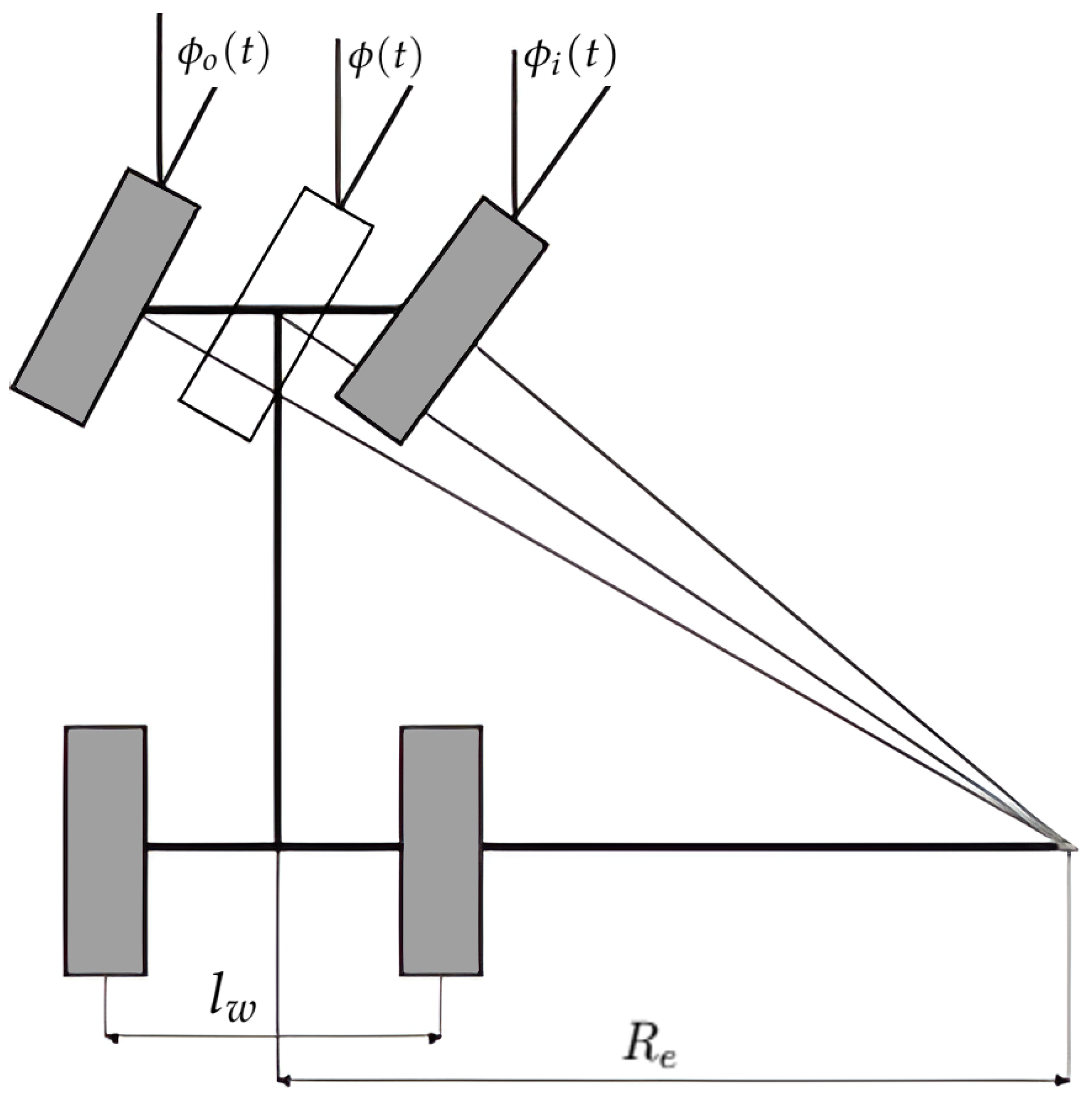
2.3. Ackermann Steering

The Ackermann steering is the most-used steering configuration in vehicles today. This is achieved by increasing the inner steering angle relative to the outer steering angle so that all tyres turn around the same point, as can be seen in Figure 1. The configuration increases stability and decreases tyre wear due to increased longitudinal slip and lateral scrubbing when compared to a parallel steering system [25]. One disadvantage is that the cornering radius at high speeds is increased, but since this paper deals with vehicles under everyday driving circumstances, this is of no concern.

Angles for the inside and outside tyre are calculated as follows:

$${\varphi }_i\left(t\right)={tan}^{-1}\left(\frac{2lsin\varphi \left(t\right)}{2lcos\varphi \left(t\right)-l_{w}sin\varphi \left(t\right)}\right)$$

(20)

$${\varphi }_o\left(t\right)={tan}^{-1}\left(\frac{2lsin\varphi \left(t\right)}{2lcos\varphi \left(t\right)+L_{w}sin\varphi \left(t\right)}\right).$$

(21)

Now that all the tyres turn around the same point, further simplification of the vehicle model is possible.

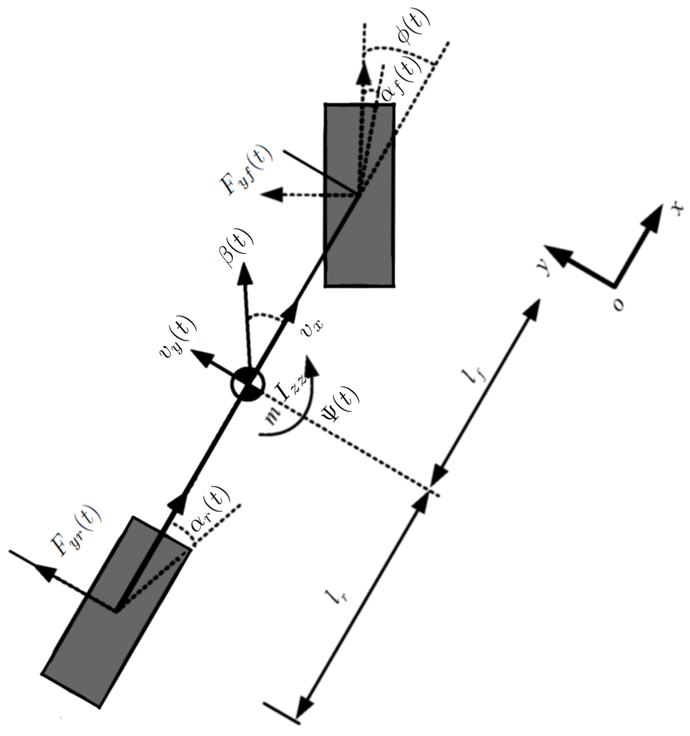
2.4. Single-Track Model

The two-degree-of-freedom single-track model (also known as the “bicycle model”) was first developed in 1940 by Riekert and Schunck [3]. This model assumes that the car can be described by only one front and one rear equivalent tyre linked by the vehicle body, as seen in Figure 2. For this assumption to work, the vehicle mass is condensed to a singular point at the centre of gravity, so that there is no pitching and rolling motion along its x and y axes and the longitudinal velocity stays constant.

From (5) and (11), we can calculate the lateral tyre forces as follows:

$$F_{yf}\left(t\right)=C_{\alpha F}{\alpha }_f\left(t\right)$$

(22)

$$F_{yr}\left(t\right)=C_{\alpha R}{\alpha }_r\left(t\right)$$

(23)

where $C_{\alpha F}$ and $C_{\alpha R}$ are the nominal cornering stiffnesses at the front and rear tyres and ${\alpha }_f\left(t\right)$ and ${\alpha }_r\left(t\right)$ are the front and rear slip angles.

$${\alpha }_f\left(t\right)=\beta \left(t\right)-ta{n}^{-1}\left(\frac{v_y\left(t\right)+\dot{\Psi }\left(t\right)l_v}{v_x}\right)-\varphi \left(t\right)$$

(24)

$${\alpha }_r\left(t\right)=\beta \left(t\right)+ta{n}^{-1}\left(\frac{v_y\left(t\right)+\dot{\Psi }\left(t\right)l_r}{v_x}\right)$$

(25)

with $\beta \left(t\right)$ being the vehicle slip angle, $\varphi \left(t\right)$ the steering angle, $v_x$ and $v_y\left(t\right)$ the longitudinal and lateral velocities, $l_a$ the distance from the front tyre to the centre of gravity, and $l_r$ the distance from the rear tyre to the centre of gravity. According to the Newton–Euler equations, the following inertial force balance equations are established:

$${\dot{v}}_y\left(t\right)m=F_{yf}\left(t\right)+F_{yr}\left(t\right)$$

(26)

$$\dot{\Psi }\left(t\right)+I_{zz}=F_{yf}\left(t\right)l_v-F_{yr}\left(t\right)l_r+M_z\left(t\right)$$

(27)

$$M_z\left(t\right)=F_{x1}\left(t\right)\frac{l_w}{2}-F_{x2}\left(t\right)\frac{l_w}{2}$$

(28)

with m being the combined mass of the vehicle and passengers, $I_{zz}$ being the moment of inertia of the vehicle around the z axis, $M_z\left(t\right)$ being the correction moment, and $F_{x1}\left(t\right)$ and $F_{x2}\left(t\right)$ being the longitudinal forces of the inner and outer rear tyres. Since we assume that the velocity is constant, it is possible to write the lateral acceleration as

$${\dot{v}}_y\left(t\right)=v_x(\dot{\Psi }\left(t\right)-\dot{\beta }\left(t\right)).$$

(29)

If we now insert Equations (22)–(25) into our equations of motion (26) and (27), we obtain:

$$v_x(\dot{\Psi }\left(t\right)-\dot{\beta }\left(t\right))m=C_{\alpha F}\left(\beta \left(t\right)-\frac{v_y\left(t\right)+\dot{\Psi }\left(t\right)l_f}{v_x}-\varphi \left(t\right)\right)+C_{\alpha R}\left(\beta \left(t\right)+\frac{v_y+\dot{\Psi }\left(t\right)l_r}{v_x}\right)$$

(30)

$$\ddot{\Psi }\left(t\right)I_{zz}=C_{\alpha F}\left(\beta \left(t\right)-\frac{v_y\left(t\right)+\dot{\Psi }\left(t\right)l_f}{v_x}-\varphi \left(t\right)\right)l_f-C_{\alpha R}\left(\beta +\frac{v_y\left(t\right)+\dot{\Psi }\left(t\right)l_r}{v_x}\right)l_r+M_z\left(t\right).$$

(31)

In order to describe the dynamic behaviour of the single-track model, a state space model is used, which can easily be derived from the equations of motion. The state space model can be written in the following way:

$$\left[\begin{array}{c}\dot{\beta }\left(t\right)\\ \ddot{\Psi }\left(t\right)\end{array}\right]=\left[\begin{array}{cc}-\frac{C_{\alpha F}+C_{\alpha R}}{m{v}_x}& \frac{m\ast v_x^2-(C_{\alpha R}b-C_{\alpha F}a)}{m{v}_x^2}\\ -\frac{C_{\alpha R}b-C_{\alpha F}a}{I_{zz}}& -\frac{C_{\alpha R}{b}^2+C_{\alpha F}{a}^2}{I_{zz}{v}_x}\end{array}\right]\left[\begin{array}{c}\beta \left(t\right)\\ \Psi \left(t\right)\end{array}\right]+\left[\begin{array}{cc}-\frac{C_{\alpha F}}{m{v}_x}& 0\\ \frac{C_{\alpha F}a}{I_{zz}}& \frac{1}{I_{zz}}\end{array}\right]\left[\begin{array}{c}\varphi \left(t\right)\\ M_z\left(t\right)\end{array}\right].$$

(32)

2.5. Self-Steering Gradient

The self-steering gradient (“$SSG$”) describes the typical steering behaviour of any given vehicle under normal circumstances, with the three $SSG$ modes being:

• $SSG>0:$ under-steering;
• $SSG=0:$ neutral;
• $SSG<0:$ oversteering.

Most consumer vehicles are set to be slightly under-steering for increased stability and safety. In this paper, the $SSG$ is used to define the desired yaw rate ${\dot{\Psi }}_d$. The $SSG$ is defined as the relationship between the steering angle $\varphi$ and the lateral acceleration ${\dot{v}}_y\left(t\right)$ and can be easily derived like this: Let us consider the following kinematic relationships:

$$\varphi \left(t\right)=\frac{l}{R\left(t\right)}+{\alpha }_f\left(t\right)-{\alpha }_r\left(t\right)$$

(33)

$$v_x=R\left(t\right)\dot{\Psi }\left(t\right)$$

(34)

$${\dot{v}}_y\left(t\right)=v_x\dot{\Psi }\left(t\right),$$

(35)

with $R\left(t\right)$ being the turning radius of the vehicle measured from the centre of gravity. Please notice that the product of $R\left(t\right)$ and $\dot{\Psi }\left(t\right)$ is constant. During steady-state cornering, all moments around the centre of gravity are zero:

$$F_{yf}\left(t\right)a-F_{yr}\left(t\right)b=0,$$

(36)

with $M_z\left(t\right)=0$. We can write this function as

$$F_{yf}\left(t\right)=m\frac{l_r}{l}{\dot{v}}_y\left(t\right)=m_f{\dot{v}}_y\left(t\right)$$

(37)

$$F_{yr}\left(t\right)=m\frac{l_f}{l}{\dot{v}}_y\left(t\right)=m_r{\dot{v}}_y\left(t\right)$$

(38)

with $m_f$ and $m_r$ are the distributed weight at the front and rear tyres. We can insert this into (33), giving us

$$\varphi \left(t\right)=\frac{l}{R\left(t\right)}+\underset{SSG}{\underbrace{\left(\frac{m_f}{C_{\alpha F}}+\frac{m_r}{C_{\alpha R}}\right)}}{\dot{v}}_y\left(t\right).$$

(39)

Seeing as we cannot measure $R\left(t\right)$ easily, we can rewrite the $SSG$ to only contain direct parameters:

$$SSG=\frac{m(C_{\alpha R}{l}_r-C_{\alpha F}{l}_f)}{C_{\alpha F}{C}_{\alpha R}l}.$$

(40)

If we now insert (34), (35), and (40) into (39) and solve for $\dot{\Psi }$, we obtain

$${\dot{\Psi }}_d\left(t\right)=\frac{v_x}{l+v_x^{2}SSG}\varphi \left(t\right)$$

(41)

with $\dot{{\Psi }_d}\left(t\right)$ being the desired yaw rate.

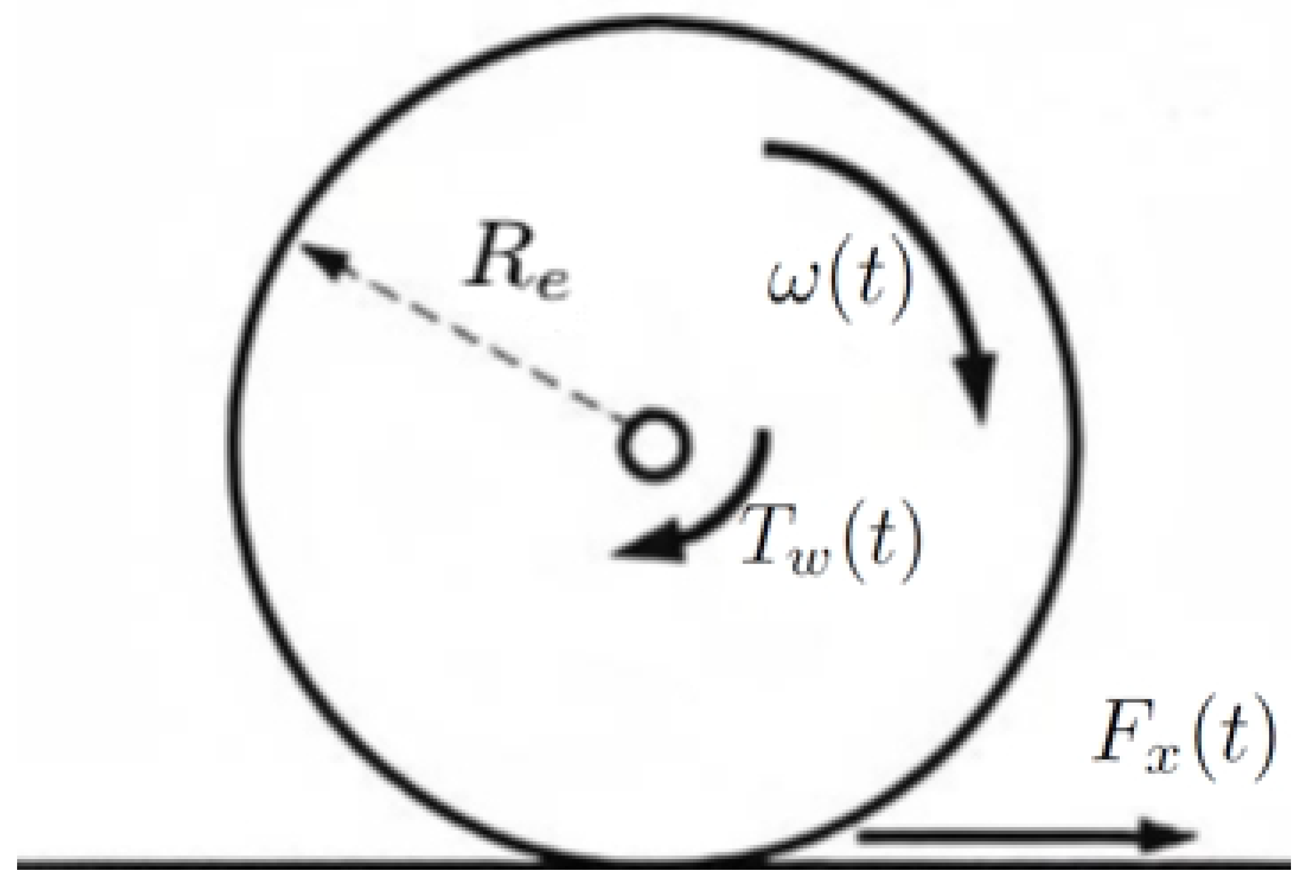
2.6. Wheel Rational Dynamics

The rotation on the wheel is the result of the interaction of the torque applied to the wheel and the forces acting against the wheel, as can be seen in Figure 3.

$$I_w\dot{\omega }\left(t\right)=T_w\left(t\right)-(F_r+F_{\Delta }\left(t\right))R_e$$

(42)

where $I_w$ is the combined moment of inertia of the wheel and the rotor of the engine, $\dot{\omega }\left(t\right)$ is the rotational acceleration of the wheel, $T_w(\left(t\right)$ is the torque applied to the wheel, $F_r$ is the constant rolling resistance, $F_{\Delta }\left(t\right)$ are the changing forces that act on the wheel that can occur due to cornering or changes in the road conditions, and $R_e$ is the effective wheel radius.

The longitudinal tyre forces are calculated similar to the lateral tyre forces:

$$F_x\left(t\right)=C_{\lambda }\lambda \left(t\right)$$

(43)

where $F_x\left(t\right)$ is the longitudinal tyre force, $C_{\lambda }\left(t\right)$ is the longitudinal wheels stiffness, and $\lambda$ is the longitudinal tyre slip. The slip for the individual rear wheels is calculated as follows:

$${\lambda }_1\left(t\right)=-\frac{(v_x+\dot{\Psi }\left(t\right)\frac{l_w}{2})-R_e{\omega }_1\left(t\right)}{v_x+\dot{\Psi }\frac{l_w}{2}}$$

(44)

$${\lambda }_2\left(t\right)=-\frac{(v_x-\dot{\Psi }\left(t\right)\frac{l_w}{2})-R_e{\omega }_2\left(t\right)}{v_x-\dot{\Psi }\frac{l_w}{2}}$$

(45)

where $\dot{\Psi }\left(t\right)$ is the yaw rate of the vehicle and ${\omega }_1\left(t\right)$ and ${\omega }_2\left(t\right)$ are the rotational velocities of the inner and outer rear tyres. If $R_e\omega \left(t\right)$ is 0, the wheel is locked and sliding occurs without rotation. If $\lambda \left(t\right)$> 0, the wheel is accelerating, and if $\lambda \left(t\right)$< 0, the wheel is breaking.

Correction Momentum and Torque

The correction momentum is the sum of all moments caused by longitudinal forces. If we now consider (28) and insert (42)–(45), we can write the correction moment as

$$M_z\left(t\right)=\left(-\frac{(v_x+\dot{\Psi }\left(t\right)\frac{l_w}{2})-R_e{\omega }_1\left(t\right)}{v_x+\dot{\Psi }\left(t\right)\frac{l_w}{2})}\right)C_{\lambda }{l}_f-\left(-\frac{(v_x-\dot{\Psi }\left(t\right)\frac{l_w}{2})-R_e{\omega }_2\left(t\right)}{v_x-\dot{\Psi }\left(t\right)\frac{l_w}{2})}\right)C_{\lambda }{l}_r.$$

(46)

The correction torque or desired torque can be calculated by solving (46) for ${\omega }_1\left(t\right)$ and ${\omega }_2\left(t\right)$, giving us:

$${\omega }_{2d}\left(t\right)=\frac{{\omega }_1\left(t\right)(v_x-\dot{\Psi }\left(t\right)\frac{l_w}{2})}{(v_x+\dot{\Psi }\left(t\right)\frac{l_w}{2})}-\frac{M_z(v_x-\dot{\Psi }\left(t\right)\frac{l_w}{2})}{C_{\lambda }{l}_r{R}_e}$$

(47)

$${\omega }_{2d}=\frac{{\omega }_1(v_x-\dot{\Psi }\frac{l_w}{2})}{(v_x+\dot{\Psi }\frac{l_w}{2})}-\frac{M_r(v_x-\dot{\Psi }\frac{l_w}{2})}{C_{\lambda }{l}_r{R}_e}$$

(48)

with ${\omega }_{1d}\left(t\right)$ and ${\omega }_{2d}\left(t\right)$ being the desired rotational wheel speeds. If we now consider (42) and insert the derivative of (47) and (48), we can solve for the desired wheel torque:

$$T_{1d}\left(t\right)=I_{\omega }{\omega }_{1d}\left(t\right)+\left((F_r+F_{\Delta })R_e\right)$$

(49)

$$T_{2d}\left(t\right)=I_{\omega }{\omega }_{2d}\left(t\right)+\left((F_r+F_{\Delta })R_e\right).$$

(50)

From here, we can insert the desired torque into the control inputs from Section 4 to control the $IM$.

3. Sliding Mode Control

Sliding Mode Control ($SMC$), or Variable Structural control ($VSC$) as it is sometimes called, is a nonlinear control strategy that applies a discontinuous signal to alter the dynamics of a system. $SMC$ was first developed in the 1960s in the Soviet Union by Emeljanov [7] and Utkin [6] based on the work of Poincaré and Lyapunov. $SMC$ systems have two distinct phases: the reaching phase and the sliding phase. During the reaching phase, the $SMC$ tries to drive the system onto the sliding surface. Once it reaches the sliding phase, the $SMC$ will try to keep the system state in the neighbourhood of the sliding surface by using a switching function. $SMC$ systems have multiple advantages. The dynamic behaviour of the system may be directly tailored by the choice of switching function; essentially, the switching function is a measure of desired performance. The control system is very robust and can be totally insensitive to matched uncertainness, which, for example, can be found in mechanical systems. Furthermore, it can be used to control linear and nonlinear systems. However, it still has disadvantages. One of the main disadvantages is the necessity of a discontinuous control signal, which needs to switch at extremely high frequencies (theoretically infinitely high) to provide reasonable rejection of uncertainty. Furthermore, the high frequency could make the usage of $SMC$ for certain electrical systems impossible. Seeing as we want the control for the electrical components, the chattering problem needs to be solved. To solve the problem, the control law needs to be a continuous function of time. One way to solve that would be to use a saturation function instead of a sign function as the switching function. However, seeing as we need to control a second-order system, the use of the “Super-Twisting” Algorithm ($STA$) becomes possible [19]. The advantage of the $STA$ is its high robustness without too much compromising on the converging speed and that its design does not depend on the knowledge of the bound values of the uncertainties disturbances [19]. That can be a huge advantage for a vehicle, as there are many external factors that can influence the driving behaviour. Some of them include differences in temperature, road surfaces, and weather. It could also be the change of air pressure, which can change the size of the contact patch and influence the driving behaviour. The main goal is to derive the sliding function $s\left(t\right)$→ 0, which is linear. In this context, the following proposition states the asymptotic stability of a sliding function using the contractive control law.

Proposition 1.

Let us consider the following sliding surface, witch only depends on the positive scalar parameter $k>0$:

$$s\left(t\right)=ϵ\left(t\right)+k{\int }_0^t\left(ϵ\left(\tau \right)\left(\tau \right)\right)d\tau ,$$

(51)

with $s\left(t\right)$ being our sliding surface and $ϵ\left(t\right)$ being the tracking error, defined as

$$ϵ\left(t\right)=\dot{\Psi }\left(t\right)-{\dot{\Psi }}_d\left(t\right),$$

(52)

then there exists a feedback control law that guarantees the asymptotic stability of the equation of motion (30).

Proof. 

Let us consider the equation of motion (30), which can be written in the following form (expressed in the state variables):

$$\ddot{\Psi }\left(t\right)=-\frac{C_{\alpha R}b-C_{\alpha F}a}{I_{zz}}\beta \left(t\right)-\frac{C_{\alpha R}{b}^2+C_{\alpha F}{a}^2}{I_{zz}{v}_x}\dot{\Psi }\left(t\right)+\frac{C_{\alpha F}{l}_f}{I_{zz}}+\frac{1}{I_{zz}}{M}_z\left(t\right).$$

(53)

If we consider (51) and (52), it follows that:

$$s\left(t\right)=\dot{\Psi }\left(t\right)-{\dot{\Psi }}_d\left(t\right)+k{\int }_0^t(\dot{\Psi }\left(\tau \right)-{\dot{\Psi }}_d\left(\tau \right))d\tau .$$

(54)

To make sure that $s\left(t\right)=0$ will be reached in a finite time, the Lyapunov approach can be used. First, we select the Lyapunov candidate:

$$V\left(s\left(t\right)\right)=\frac{1}{2}s{\left(t\right)}^2,$$

(55)

from which follows

$$\dot{V}\left(s\left(t\right)\right)=\dot{s}\left(t\right)s\left(t\right)$$

(56)

$$\dot{V}\left(s\left(t\right)\right)=(\ddot{\Psi }\left(t\right)-{\ddot{\Psi }}_d\left(t\right)+k(\dot{\Psi }\left(t\right)-{\dot{\Psi }}_d\left(t\right)))s\left(t\right).$$

(57)

The control output consists of two parts:

$$u\left(t\right)=u_{eq}\left(t\right)+u_{cor}\left(t\right)$$

(58)

where $u_{eq}\left(t\right)$ is the equivalent output and $u_{\mathrm{cor}}\left(t\right)$ is the corrective output that keeps $SMC$ on the sliding surface. $u_{eq}\left(t\right)$ can be easily calculated by setting $\dot{V}\left(t\right)=0$ and solving for the output $M_z\left(t\right)$. If we now consider the yaw motion equations:

$$\ddot{\Psi }\left(t\right)=-\frac{C_{\alpha R}b-C_{\alpha F}a}{I_{zz}}\beta \left(t\right)-\frac{C_{\alpha R}{b}^2+C_{\alpha F}{a}^2}{I_{zz}{v}_x}\dot{\Psi }\left(t\right)+\frac{C_{\alpha F}{l}_f}{I_{zz}}\Phi \left(t\right)+\frac{1}{I_{zz}}{M}_z\left(t\right)$$

(59)

$$u_{eq}\left(t\right)=M_z\left(t\right)$$

(60)

where

$$\begin{array}{cc}\hfill M_z\left(t\right)=C_{\alpha R}b-C_{\alpha F}\beta \left(t\right)+\frac{C_{\alpha R}{b}^2+C_{\alpha F}{a}^2}{v_x}\dot{\Psi }\left(t\right)& -C_{\alpha F}{l}_f\Phi \hfill \\ & +[{\ddot{\Psi }}_d\left(t\right)-k(\dot{\Psi }\left(t\right)-{\dot{\Psi }}_d\left(t\right))s\left(t\right)]I_{zz}.\hfill \end{array}$$

(61)

Imposing that

$$\dot{V}\left(s\left(t\right)\right)<0,$$

(62)

and to satisfy (62), the following corrective part of the control input in the context of STA can be considered:

$$u_{\mathrm{cor}}\left(t\right)=-\sqrt{U}\sqrt{\left|s\right(t\left)\right|}sgn\left(s\left(t\right)\right)+\xi \left(t\right)$$

(63)

$$\dot{\xi }\left(t\right)=-Wsgn\left(s\left(t\right)\right),$$

(64)

where U and W are two positive constants that should be manually tuned to be large enough to ensure a good performance. □

Remark 1.

Typically (see [20]), $W\approx 1.1 \mathrm{U}$ to obtain in general good dynamical performance. As we can see in Figure 4, the STA behaves similarly to a PI controller [20], with the big difference being that the STA uses a sigmoid function instead of a proportional function.

4. Analysis and Discussion of the Results

All simulations were preformed in MATLAB SIMULINK®. The Basic control strategy that was used in all simulations can be seen in Figure 5. For the analysis of the system and the controller, a series of different scenarios was simulated. All simulations were run with a constant steering angle of 10° or a steering angle as a sine wave input with an amplitude of 10° and a frequency of $1\frac{\mathrm{rad}}{\mathrm{s}}$, with a sample time of 10 s. Later on, the disturbance was always applied to $F_{\Delta 1}\left(t\right)$. The disturbance signal was a uniform random number with an upper bound of $\left|20\right| \mathrm{N}$ and a sample time of 0.1 s and the seed set to 0. A uniform random number with seed was chosen to provide repeatability for testing.

The analysis of the system was performed with the following vehicle and $IM$ constants, see

Table 3. Vehicle constants.

m	2100 kg
$I_{zz}$	2800 kg m${}^2$
$l_f$	2 m
$v_x$	15 m/s
$l_r$	3 m
$F_r$	80 N
$l_w$	1.8 m
$C_{aF}$	75,000 $\frac{N}{deg}$
$C_{aR}$	150,000 $\frac{N}{deg}$
$C_{\lambda }$	−15,000 $\frac{N}{\lambda }$

and

Table 4. IM constants.

Pole Number	6
$f_{max}$	50 Hz
$f_{max}$	$\frac{400}{\sqrt{3}}$ V
$R_1$	0.182 $\Omega$
$X_1$	0.990 $\Omega$
$X_2$	0.180 $\Omega$
$X_m$	7.4 $\Omega$

.

The following gains of the SMC STA and PI controller were used, see

Table 5. Controller gains.

	STA/SMC Overestimated	STA/SMC Underestimated
U	100	15
k	500	500
	PI Controller
P	−1000	N/A
I	−800	N/A

.

4.1. Simulation of an Uncontrolled and Undisturbed System

In the first test, the system was left uncontrolled and no disturbances were applied, first, the constant steering angle and, after that, the sine wave input.

In Figure 6 and Figure 7, the difference between the yaw rate and the desired yaw rate can be observed. This is mainly caused by the high moment of inertia of the vehicle. These two graphs served as the baseline for the further tests.

4.2. Simulation of a Controlled Undisturbed System

For this test, k and U were set to $k=500$ and $U=100$. The system was controlled by the SMC, and no disturbance was applied.

If we now compare the results from Figure 6 (the uncontrolled test) with the results of the controlled test in Figure 8, we can see a drastic improvement. If we would zoom in on a maximum, we can see a slight error between the desired yaw rate and the current yaw rate, as seen in Figure 9. This error is the highest at the maxima with an error of about $0.004$ $\frac{\mathrm{rad}}{\mathrm{s}}$, which can be neglected, considering that $0.004$ $\frac{\mathrm{rad}}{\mathrm{s}}$ is approximately equal to $2.3$ rotations per hour.

As can be seen in Figure 10 and Figure 11, the system performed worse if compared to the uncontrolled test with no disturbance in Figure 6, with much variation in the yaw rate, which would cause an unpleasant driving experience. This becomes even more apparent if we apply the same disturbance to a system with a constant steering angle.

4.3. Simulation of a Controlled and Disturbed System

To show the effectiveness of $SMC$, the system was left uncontrolled and the disturbance was applied. If we now apply $SMC$ to the disturbed system, we obtain the following.

The performance of the system was quite similar to the controlled system with no disturbance in Figure 8. It even went down to a similar error of about $0.004\frac{\mathrm{rad}}{\mathrm{s}}$ in Figure 12. If we look at the maximum of the system and compare it to Figure 9, we can see a slight variation over time of about $0.0002\frac{\mathrm{rad}}{\mathrm{s}}$, which, again, is negligible.

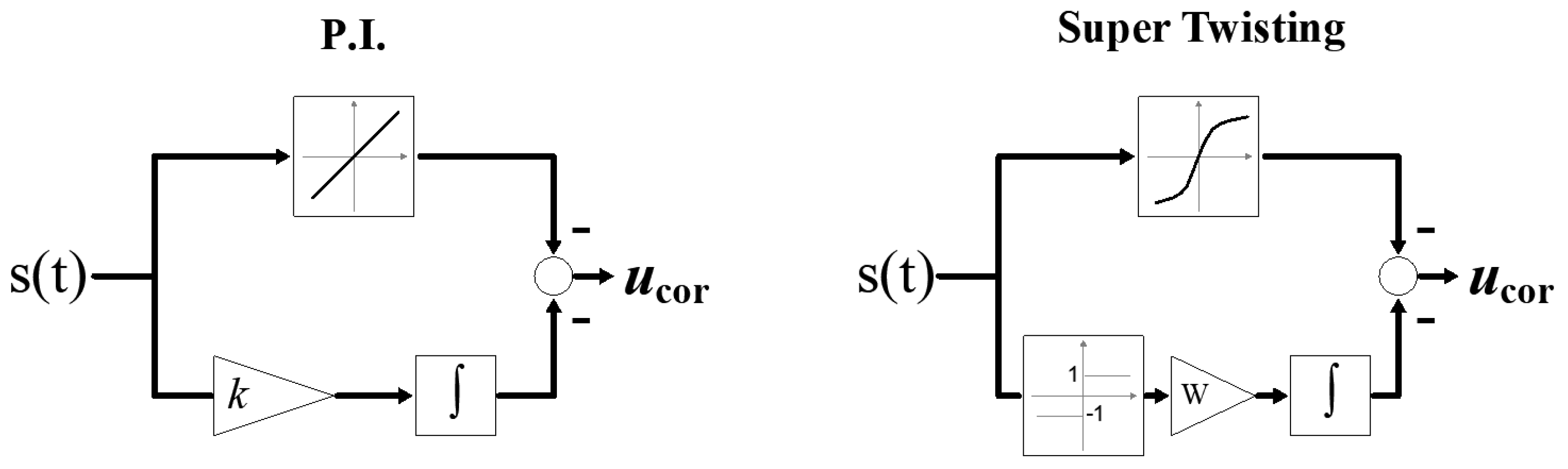
PI Controller vs. SMC Super-Twisting

During initial testing of a system, a $PI$ controller was used. These testes were carried out without any disturbance and produced good results. Due to the high stiffness of the system, the proportional gain was set to $P=-1000$ and the integral gain was set to $I=-800$. While initially, it showed promising results, the moment the disturbance was applied, the weakness of the $PI$ controller was revealed.

As can be clearly seen in Figure 13, the controller was not able to control the system adequately. While it behaved better than the uncontrolled disturbed system, as seen in Figure 10, it was nowhere close to the performance that can be seen in Figure 12.

Comparing the PI controller to the SMC strategy is not a fair task. In any case, some structural considerations can be made. The PI controller is one of the oldest and simplest controller that we can find in industrial applications. The PI controller can be used for linear and nonlinear systems, and its success and longevity are due to its easy, cheap, and direct application. In its basic structure, the PI controller is a signal-based controller. In this sense, it is quite a robust controller, but the difficulty that it presents is that it is not easy to tune. In fact, in accordance with the stability and the robustness of the closed-loop scheme, the tuning procedure plays a key role. SMC presents also high stability and robust quality due to its corrective part; see [9]. The advantage of SMC is that it is structurally straightforward to prove the stability and the robustness of the closed-loop control system assuming that the upper and lower bounds of the uncertainties, including the disturbance, are known. In case these bounds are not known, then an STA can be applied; see [20]. In fact, in this context, the control strategy works also without knowledge of these bounds.

4.4. SMC vs. STA

As was already stated, one of the main benefits of the $STA$ is that the upper bounds of the disturbances are not required to be known. This becomes very useful if the upper bounds of the disturbances are not known. We can compare the $STA$ to normal $SMC$ with the corrective input defined as

$$u_{\mathrm{cor}}\left(t\right)=Usgn\left(s\left(t\right)\right).$$

(65)

In comparing $SMC$ with the $STA$, both controllers used the same k and U as in the tests before, giving us the following results.

As can be seen in Figure 14, the yaw rate of the system with $SMC$ constantly stays higher than the desired yaw rate. The $STA$-controlled system (see Figure 15) varied more over time. While the error for both of them was quite small, a bigger problem was revealed when the sliding surfaces of Figure 14 and Figure 15 were compared.

If we compare the sliding surface of $SMC$ (Figure 16) and the $STA$ (Figure 17), were can immediately see that, without the known upper bounds of the disturbances, the sliding surface of $SMC$ constantly increased, and it was not able to keep nor steer $s\left(t\right)\to 0$. While the $STA$ is not perfect, it was able to keep $s\left(t\right)$ near 0, which would be still good enough for our purposes.

4.4.1. SMC with Known Upper Bounds

If we assume that the upper bounds of the disturbances are knowable, meaning

$$u_{\mathrm{cor}}\left(t\right)=\lceil F_{\Delta }\rceil U\mathrm{sgn}\left(s\left(t\right)\right)$$

(66)

the $SMC$ has a better performance (Figure 18) if compared to Figure 14. Furthermore, the sliding surface of Figure 19 performs better than $SMC$ (Figure 16) without known upper bounds or the $STA$ in Figure 17. However, with this, we ran into the so-called chattering problem. As already stated, the high frequency makes it impossible to use it for certain electrical systems [21].

4.4.2. Achievability

Another problem we might have is the question of achievability. While $C_{\lambda }$ is relatively big at $-15,000\frac{\mathrm{N}}{\lambda }$, for the control output, a longitudinal slip of ${\lambda }_1=0.74$ is required for both wheels to achieve the required maximal correction moment of $M_z=\mathrm{20,000}\mathrm{N}$, see Figure 20. While this is still possible to achieve, it is highly ineffective. If we compare it to the correction moment of the $STA$ (Figure 21), a much lower momentum is needed for a similar performance.

Generally, it can be said that the $STA$ is less accurate than $SMC$. Precision accuracy is not necessarily needed as this design is intended for consumer vehicles. It is more important to have a smoother continuous control signal than a fast and accurate one.

If we compare $SMC$ and the $STA$ in their energetic error over a period of time of $t=0\to t=10$ by calculating

$$e_{\Delta }={\int }_0^tϵ{\left(\tau \right)}^{2}d\tau$$

(67)

we obtain an energetic error for $SMC$ of $e_{\Delta }=0.00269$ and for the $STA$ of $e_{\Delta }=0.00558$. While the energetic error of the $STA$ was worse, if we compare $SMC$ (Figure 18) and the $STA$ (Figure 15) in regard to the maximum error, we can see that the $SMC$ had a maximum error of $0.01\frac{\mathrm{rad}}{\mathrm{s}}$ and the $STA$ a maximum error of $0.005\frac{\mathrm{rad}}{\mathrm{s}}$.

4.4.3. SMC and STA with Underestimated Correctiveness

To show the ability of of the $STA$ to perform without knowing the upper bound of the error, the corrective part was set to be $U=15$. This test was both performed first with the $STA$ and then with $SMC$. This test was performed for a duration of 200 seconds to better show the performance of both controllers.

In both cases, the error was larger than with the well-estimated corrective part, with the difference being that the $STA$ (Figure 22) had a trend toward the desired value, while $SMC$ (Figure 23) stayed constant over the desired yaw rate. In terms of the energetic error, the $STA$ performed better with an energetic error of $e_{\Delta }=0.002971$ and $SMC$ with an energetic error of $e_{\Delta }=0.004319$. Both had a maximal error of $0.007\frac{\mathrm{rad}}{\mathrm{s}}$. We compared the results of this test with the one performed before, see

Table 6. Results.

	STA Overestimated	STA Underestimated
Energetic error	0.00558	0.002971
Maximum error	0.005 $\frac{\mathrm{rad}}{\mathrm{s}}$	0.007 $\frac{\mathrm{rad}}{\mathrm{s}}$
	SMC Overestimated	SMC Underestimated
Energetic error	0.002971	0.004319
Maximum error	0.001 $\frac{\mathrm{rad}}{\mathrm{s}}$	0.007 $\frac{\mathrm{rad}}{\mathrm{s}}$

.

As can be clearly seen from the table, the $STA$ was able to perform better than $SMC$ in this case, thus proving that the $STA$ is able to perform without the upper bounds being known.

5. Conclusions

This paper explored the possibility to use two $IM$s and $SMC$ with the $STA$ to replace the differential gear in a consumer vehicle. While a real measurement of a model vehicle was not possible as originally planned for this paper, the results are promising. The yaw rate of the vehicle aligned with what can be found in [4], which originally was the biggest problem to overcome due to the numerous errors that could be found in some of the originally consider literature. $SMC$ has shown a great capability to control the system under different circumstances and even outperforming the classic $PI$ controller. Some similar results also were found in [20]. The capability of the $STA$ to solve the chattering phenomena problem while keeping the robustness of the $SMC$ intact is surprising, as it was a later addition to the paper, and first, a standard $SMC$ approach was chosen. While $SMC$ with the $STA$ was not able to slide perfectly, the resulting error was still very small, especially considering the speed of the disturbance. Its ability to perform even without knowing the upper bounds of the disturbance makes it a very valuable control tool. As the model in this paper was heavily simplified and highly linear, a real vehicle might perform differently, which would be interesting to test the theoretical knowledge on a real vehicle to see if the theory translates into praxis. Theoretically, it could perform even better due to the nonlinearity of the tyres, as rapid changes in momentum and acceleration are no longer possible. Furthermore, it was interesting to see the interactions of the different parts of the vehicle model and $SMC$ and the $STA$. While a more in-depth look into all parts of this paper would be highly interesting, it would go beyond the scope of this paper. The impact of longitudinal motion on the controller would especially be of high interest and/or the behaviour of the controller in extreme situations, as described in [4].

References

1. De Novellis, L.; Sorniotti, A.; Gruber, P. Wheel Torque Distribution Criteria for Electric Vehicles with Torque-Vectoring Differentials. IEEE Trans. Veh. Technol. 2014, 63, 1593–1602. [Google Scholar] [CrossRef] [Green Version]
2. Pacejka, H.B. Tyre and Vehicle Dynamics; Butterworth-Heinemann: Oxford, UK, 2006. [Google Scholar]
3. Riekert, P.; Schunck, T. Zur Fahrmechanik des gummibereiften Kraftfahrzeugs. Ingenieur-Archiv 1940, 11, 210–224. [Google Scholar] [CrossRef]
4. von Vietinghoff, A. Nichtlineare Regelung von Kraftfahrzeugen in Querdynamisch Kritischen Fahrsituationen; Universitätsverlag Karlsruhe: Karlsruhe, Germany, 2008. [Google Scholar]
5. Bahram, A. Induction Motors Analysis and Torque Control; Springer: Berlin/Heidelberg, Germany, 2001. [Google Scholar]
6. Utkin, V.I. Variable Structure Systems with Sliding Modes. IEEE Trans. Autom. Control 1977, 22, 212–222. [Google Scholar] [CrossRef]
7. Emelyanov, S.V. Automatische Regelsysteme Mit Veranderlicher Struktur Fahrsituationen; Oldenbourg: Munich, Germany, 1969. [Google Scholar]
8. Lyapunov, A.M. The General Problem of the Stability of Motion; CRC Press: Boca Raton, FL, USA, 1992. [Google Scholar]
9. Slotine, J.J.E.; Li, W. Applied Nonlinear Control; Pearson: Upper Saddle River, NJ, USA, 1991. [Google Scholar]
10. Liu, J.; Wang, X. Advanced Sliding Mode Control. In Advanced Sliding Mode Control for Mechanical Systems: Design, Analysis and MATLAB Simulation; Springer: Berlin/Heidelberg, Germany, 2011. [Google Scholar]
11. Mercorelli, P. An Anti-Saturating Adaptive Preaction and a Slide Surface to Achieve Soft Landing Control for Electromagnetic Actuators. IEEE/ASME Trans. Mechatron. 2012, 17, 76–85. [Google Scholar] [CrossRef]
12. Liu, J.; Li, H.; Deng, Y. Torque Ripple Minimization of PMSM Based on Robust ILC Via Adaptive Sliding Mode Control. IEEE Trans. Power Electron. 2018, 33, 3655–3671. [Google Scholar] [CrossRef]
13. Jezernik, K.; Korelič, J.; Horvat, R. PMSM sliding mode FPGA-based control for torque ripple reduction. IEEE Trans. Power Electron. 2013, 28, 3549–3556. [Google Scholar] [CrossRef]
14. Haus, B.; Röhl, J.H.; Mercorelli, P.; Aschemann, H. Model Predictive Control for Switching Gain Adaptation in a Sliding Mode Controller of a DC Drive with Nonlinear Friction. In Proceedings of the 2018 22nd International Conference on System Theory, Control and Computing (ICSTCC), Sinaia, Romania, 10–12 October 2018; pp. 765–770. [Google Scholar] [CrossRef]
15. Haus, B.; Mercorelli, P.; Aschemann, H. Gain Adaptation in Sliding Mode Control Using Model Predictive Control and Disturbance Compensation with Application to Actuators. Information 2019, 10, 182. [Google Scholar] [CrossRef] [Green Version]
16. Mercorelli, P.; Haus, B.; Zattoni, E.; Aschemann, H.; Ferrara, A. Robust Current Decoupling in a Permanent Magnet Motor Combining a Geometric Method and SMC. In Proceedings of the 2018 IEEE Conference on Control Technology and Applications (CCTA), Copenhagen, Denmark, 21–24 August 2018; pp. 939–944. [Google Scholar] [CrossRef]
17. Haus, B.; Aschemann, H.; Mercorelli, P.; Werner, N. Nonlinear modelling and sliding mode control of a piezo-hydraulic valve system. In Proceedings of the 2016 21st International Conference on Methods and Models in Automation and Robotics (MMAR), Miedzyzdroje, Poland, 29 August–1 September 2016; pp. 442–447. [Google Scholar] [CrossRef]
18. Aschemann, H.; Haus, B.; Mercorelli, P. Sliding Mode Control and Observer-Based Disturbance Compensation for a Permanent Magnet Linear Motor. In Proceedings of the 2018 Annual American Control Conference (ACC), Milwaukee, WI, USA, 27–29 June 2018; pp. 4141–4146. [Google Scholar] [CrossRef]
19. Dimna Denny, C.; Ramesh Kumar, P.; Jasmin, E.A. Super Twisting Algorithm Based Slip Ratio Control of Electric Vehicles. In Proceedings of the 2020 IEEE International Power and Renewable Energy Conference, Karunagappally, India, 30 October–1 November 2020; pp. 1–6. [Google Scholar] [CrossRef]
20. Xu, C.; Wang, K.; Wang, Y.; Chen, C.; Zhang, B. Super-Twisting Sliding Mode Control of Permanent Magnet Synchronous Motor Based on Predictive Adaptive Law. In Proceedings of the 2021 IEEE 5th Advanced Information Technology, Electronic and Automation Control Conference (IAEAC), Chongqing, China, 12–14 March 2021; Volume 5, pp. 2731–2736. [Google Scholar] [CrossRef]
21. Benariba, H.; Boumédiène, A. Super twisting sliding mode control of an electric vehicle. In Proceedings of the 2015 3rd International Conference on Control, Engineering Information Technology (CEIT), Tlemcen, Algeria, 25–27 May 2015; pp. 1–6. [Google Scholar] [CrossRef]
22. Liu, Y.C.; Laghrouche, S.; N’Diaye, A.; Cirrincione, M. Hermite neural network-based second-order sliding-mode control of synchronous reluctance motor drive systems. J. Frankl. Inst. 2021, 358, 400–427. [Google Scholar] [CrossRef]
23. Biricik, S.; Komurcugil, H.; Ahmed, H.; Babaei, E. Super Twisting Sliding-Mode Control of DVR With Frequency-Adaptive Brockett Oscillator. IEEE Trans. Ind. Electron. 2021, 68, 10730–10739. [Google Scholar] [CrossRef]
24. Tran, M.T.; Lee, D.H.; Chakir, S.; Kim, Y.B. A Novel Adaptive Super-Twisting Sliding Mode Control Scheme with Time-Delay Estimation for a Single Ducted-Fan Unmanned Aerial Vehicle. Actuators 2021, 10, 54. [Google Scholar] [CrossRef]
25. Milliken, W.F. Race Car Vehicle Dynamics; Society of Automotive Engineers: Warendale, PA, USA, 1995. [Google Scholar]
Figure 1. Ackermann steering system.
Electronics 11 01330 g001
Figure 2. Single-track model.
Electronics 11 01330 g002
Figure 3. Basic dynamics of a tyre.
Electronics 11 01330 g003
Figure 4. Block diagram of PI (left) and super-twisting (right) controllers.
Electronics 11 01330 g004
Figure 5. Basic control strategy.
Electronics 11 01330 g005
Figure 6. Uncontrolled yaw rates with no disturbance sine input.
Electronics 11 01330 g006
Figure 7. Uncontrolled yaw rates with no disturbance uncontrolled constant input.
Electronics 11 01330 g007
Figure 8. Controlled yaw rates with no disturbance with sine wave input.
Electronics 11 01330 g008
Figure 9. Controlled yaw rates with no disturbance with sine wave input, zoomed in.
Electronics 11 01330 g009
Figure 10. Uncontrolled yaw rates with disturbance with sine wave input.
Electronics 11 01330 g010
Figure 11. Uncontrolled Yaw rates with disturbance with constant input.
Electronics 11 01330 g011
Figure 12. Controlled yaw rates with disturbance with constant input.
Electronics 11 01330 g012
Figure 13. PI-controlled yaw rates with disturbance with sine wave input.
Electronics 11 01330 g013
Figure 14. Controlled yaw rates with SMC and constant input.
Electronics 11 01330 g014
Figure 15. Controlled yaw rates with disturbance with constant input.
Electronics 11 01330 g015
Figure 16. Sliding surface SMC and constant input.
Electronics 11 01330 g016
Figure 17. Sliding surface STA and constant input.
Electronics 11 01330 g017
Figure 18. Controlled yaw rate with SMC and upper bounds known.
Electronics 11 01330 g018
Figure 19. Sliding surface SMC and upper bounds known with constant input.
Electronics 11 01330 g019
Figure 20. Control output of SMC upper bounds known.
Electronics 11 01330 g020
Figure 21. Control output of the STA.
Electronics 11 01330 g021
Figure 22. STA with underestimated value.
Electronics 11 01330 g022
Figure 23. SMC with underestimated value.
Electronics 11 01330 g023