Modeling and Performance Evaluation of Multi-Class Queuing System with QoS and Priority Constraints

Abstract

Many service providers often categorize their users into multi-classes, depending on their service requirements. Each class has strict quality of service (QoS) demands (e.g., minimum required service rate or transfer time) that must be ensured throughout its service. In some cases, priorities are also assigned in a multi-class user’s environment to ensure that the important class user shall be serviced first. In this paper, we have developed a novel Markov chain based analytical model to investigate and evaluate a multi-class queuing system with a strict QoS requirement and priority constraints. Experimental analysis is conducted for two users classes, i.e., class-1 (may be free/student users) and class-2 (may be paid/research users). Each class requests have strict QoS requirements in terms of the minimum required rate (MRR) that must be ensured throughout its lifetime once the request is admitted into the system. Secondly, class-2 requests have preemption priority over class-1, i.e., if there is no room for newly arriving class-2 requests, then one or more active flows of class-1 can be ejected in order to accommodate high-class requests. Model results are validated through simulation results and performance measures of our interest include blocking probability (BP) of individual classes and the overall system, effect of higher-class jobs on lower-class jobs, and link capacity utilization. The proposed model can be instrumental in developing advanced connection admission control (CAC), efficient resource dimensioning, and capacity planning of the queuing system.

1. Introduction

Communication and information technologies have made tremendous growth in the recent past. At the same time, many scientific and non-scientific applications are putting complex demands on these networks. Grid and Cloud computation technologies offer many useful applications that are based on high-speed computation and communication [1]. Some of these applications require data transmission to be completed within certain time bounds while others demand certain QoS to be maintained throughout its service [2,3,4]. The network resources are often shared among various users and they may be assigned priorities over one another (preemptive and non-preemptive) [5,6]. Moreover, network resource dimensioning and capacity planning needs to be done efficiently, depending on the arriving traffic rate and pattern. In short, complex user demands and growing technologies offer too many challenges for the researchers to find a match between the two and they have attracted a lot of research attention. Mathematical and analytical modeling techniques have proven to be an effective and ideal tool for capturing these system behaviors and undertaking performance evaluations under varying conditions.

Grid/Cloud computing environment provides an abstract view of the underlying resources and seamless representation as a single entity to end-user [7]. The users just need to focus on their tasks without worrying about the underlying architecture. The resources may include supercomputing devices, large storage capacities, and high-speed communication links, etc. In cases where the resource’s placement is geographically distributed, we can only estimate the capacity of bottleneck link along the path of data transfer, but no control over the traffic and its allocation. For capacity planning and network dimensioning, we consider such a Grid/Cloud computing environment, where all of the resources are under the control of a single, centralized entity, e.g., Grid’5000 [8].

Any new system or proposed technique can be evaluated for correctness and effectiveness in three different ways.

• Real Implementation: this is done by performing a real experiment on designated tools and devices. Although this approach will give us the exact results but it involves too much labor and cost (in terms of time and money). Moreover, the design may often require slight modification and tuning, but this approach is not flexible enough to accommodate these minor adjustments, and it will result in an increase in cost and delay. Therefore, this is not the best way to start with.
• Simulation: this is done by performing simulations using simulators that closely reflect real-world intended scenarios. Although, the simulator may not capture exactly all real-world parameters and, hence, its results may be slightly different than the true results, but still gives nice insight into the system behavior. The simulation models are easy to be developed and used to have a quick initial glance of system behavior with proposed modifications. The parameters can be easily fine-tuned to achieve optimal results at zero cost. Simulators can be used as an effective start-up tool, but their results cannot be fully trusted, as they may not capture the exact real world.
• Analytical Modeling: this is done by developing a mathematical model of the intended system and then the model can be used to evaluate the performance of a system under varying conditions to analyze its behavior. These models are often based on certain assumptions regarding some of the system parameters that are often criticized and considered as a flaw. In reality, anything other than real implementation is based on some assumptions in one way or the other. The assumptions are not just made blindly, rather they are supported by strong and valid arguments. Assumptions are based on a closed approximation of the real-world conditions.

Simulation modeling and analytical modeling are both considered to be the most efficient way of doing initial performance analysis and are often used in conjunction to validate each other. They are useful where the real system is not existing and yet to be developed. Once a technique is proven working through modeling and simulation, then its success is also more likely in real implementations.

Modeling and performance evaluation of multi-class queuing networks has gained a lot of research attention [9,10,11,12]. Typically, network system models are mostly based on Markov Chains. The bottleneck link can be viewed as a Single Server Queue and solved using Continuous Time Markov Chain (CTMC). Laplace and Fourier’s transformations are also frequently used in the solution of these queues. Some researchers have used the concept of Linear Programming by mapping this bottleneck link utilization problem to an optimization problem. Petri-nets are used in modeling scientific workflows that enable scientists to describe their work as a series of tasks without worrying about resource allocation and coordination. Several solution techniques can be found in [13,14,15,16].

This research is mainly aimed at developing a novel analytical model that is flexible enough to capture network behavior under multi-class flows with strict QoS requirements, such as deadline and priority constraints in Grid/Cloud networks. This work is an extension of our previous study [17] in which, we have presented an analytical model for multi-class deadline constrained data transfer without considering preemption priorities. To the best of our knowledge, no such model has been developed until the write-up of this document, which can capture multi-class queuing system behavior with strict QoS demands and priority constraints. The proposed model is a representation of a system with multi-class users; each having certain priority and QoS constraints. An example of such a system can easily be found in several daily life queuing systems. For the sake of demonstration, we restrict our study to Grid/Cloud computing environment and the same can be extended/applicable to any queuing system with stated characteristics. Furthermore, we consider the Grid/Cloud computing environment with dedicated communication lines, because the model is only applicable where the notion of QoS is valid, while the traditional Internet is known for its best-effort services. Our goal is to design an integrated and unified model that can be used for performance evaluation of the system with multi-class users having a deadline and priority constraints. The proposed model will be useful in high-speed network dimensioning, QoS provisioning, and capacity planning.

The rest of the text is organized, as follows: Section 2 presents a brief review of related work. Section 3 presents a brief description of the network systems and their corresponding characteristics. Section 5 depicts our proposed model. Section 6 presents the performance analysis. The paper is concluded in Section 7, with an outlook to our future work.

2. Related Work

With the advancement in communication and information technology, users and organization QoS demands are also growing and becoming more challenging. This section presents a brief review of various related models proposed in the literature. Each model captures network behavior under different conditions and user requirements. Bonald et al. conducted performance modeling and analysis of elastic flows in [18]; however, deadline constraints are not included in their proposed model. They have modeled the bottleneck link as an M/G/1-PS queue for fairness analysis and onward mean throughput approximation of TCP protocol. Bandwidth dimensioning model was developed by Berger et al. in [19] to estimate bandwidth share of individual connection in high-speed networks. They have considered a single bottleneck link in the network. Operations in semiconductor manufacturing are modeled as M/M(a,b)/c/PR priority queue by the authors of [20]. They have considered two priority classes without modeling deadline constraints. AlQahtani et al. developed an analytical model for 3G wireless networks for performance analysis of various control schemes in [21]. They have analyzed four different traffic classes, i.e., two non-real-time and two real-time.

Fodor G. et al. developed a model to estimate throughput guarantees and compute blocking probabilities for three kinds of flows in [22] i.e., (a) Rigid/Non-adaptive streaming flows with strict throughput requirement, e.g., voice calls, (b) adaptive streaming flows has a peak bandwidth requirement $b_2$, but they can be squeezed down to $b_2^{min}$ to accommodate other flows. Their holding time is independent of allocated $BW$ e.g., an adaptive video flow with codec enabled, and (c) elastic flows have lower and upper throughput bounds. The model is based on the extension of the classical loss model that was originally designed for ATM and circuit-switched networks. The concept of Partial Overlap (POL) is used in this model to divide the available capacity into two (1) $B{W}_{com}$ reserved for rigid flows (2) $B{W}_{ELS}$ reserved for Elastic and Adaptive flows. According to [22], the acceptable blocking probability threshold for each class is assumed as $B{P}_1^{max}$, $B{P}_2^{max}$ and $B{P}_3^{max}$ and $N_1$, $N_2$ and $N_3$ are the max no. of jobs of each class that can be accommodated, respectively. Because $B{W}_{com}$ is dependent upon $B{P}_1^{max}$ and it can be calculated easily using the Erlang-B formula. After fixing $B{W}_{com}$, we can calculate the max. no. of jobs of rigid flows $N_1$ as

$$N_1=\frac{B{W}_{com}}{b_1}$$

(1)

where $b_1$ is the peak bandwidth requirement of individual rigid flow.

The values of $N_2$ and $N_3$ are iteratively calculated using an algorithm, called the Iterative Link Allocation procedure. The algorithm starts with some large values of $N_2$ and $N_3$, and it calculates their respective blocking probabilities $B{P}_2^{max}$ and $B{P}_3^{max}$ using CTMC. The values of $N_2$ and $N_3$ are decremented after every iteration until it results in such values for which $B{P}_2\le B{P}_2^{max}$ and $BP3\le B{P}_3^{max}$. It aims at establishing a trade-off between $BP$ and throughput as larger values of $N_2$ and $N_3$ will certainly reduce their respective $BP$, but it will result in their throughput degradation. In [23], the authors proposed an Autonomic Distributed Streaming Service (ADSS) model for the application that involves data streaming between remote systems with/without in-transit data processing. The proposed ADSS model enables the intermediate node to change their behavior in response to the environmental conditions, i.e., network congestion or destination receiving rate. In such cases, ADSS can opportunistically exploit intermediate processing nodes in order to perform partial/complete in-transit processing on data, or it can temporarily store the data into the hard disk to avoid buffer overflow and data loss. Provided that data arrival rate at an intermediate node is $\lambda$, now, depending upon the reception rate of next-hop node and network congestion level, ADSS will automatically exploit perform in-transit processing on data at rate $\mu$ or temporarily store the data onto a hard disk with the rate $\omega$. The model takes current values $\lambda$, $\mu$, and $\omega$ as input and calculates future values for $\mu$, $\omega$, and the number of processing units to use for the next interval of time. ADSS is implemented using Reference Net (a kind of Petri-Nets) that helps in achieving required synchronization between associating processing nodes. The model applies to applications with end-to-end QoS requirements and can combine in-transit processing with data transmission.

Network slicing and software-defined networking (SDN) are the two most commonly used solutions for provisioning QoS in 5G networks. However, the efficient utilization of the network resources requires precise modeling of the traffic. Santhosha et al. developed a multi-class network model using SDN and network slicing to quantify network performance [24]. Heterogeneous flows are assumed from customers with different varying intensities without considering the deadline or priority constraints. A simulation-based model is presented in [25] in order to study the stability region in multi-class queuing networks. The requests are processed based on the first-come-first-serve policy without having priorities. Baris et al. studied the abandonment behavior of multi-class customers due to network congestion in [26]. Each class customer request receives different reward and cost rates, and their proposed model attempts to maximize their expected utilities. Likewise, many other studies can be found in the literature with emphasis on multi-class traffic modeling [27,28,29]. However, none of these studies consider deadline constrained bulk data transfers with preemptive priorities. Rami et al. studied the multi-class queuing system with dynamic priorities that are dependent upon the workload without considering the deadline constraints [30]. An improved scheduling policy is presented in [31] for a real-time queuing system with rewards and deadlines while ignoring the priorities.

In [32], the authors considered a multi-server queuing system with three priority classes and two servers. Each class of customers has its arrivals and service rates. They have used numerical analysis methods to solve the system of linear equations and calculate each class blocking probability and average queue length using system steady-state probabilities. Kannan et al. worked on scheduling bulk file transfers with deadline constraints by dividing the time scale into uniform time slices [33]. Bandwidth adjustments are made at the start of every time slice. They have also explored file transfer over multi-paths and found significant improvement in throughput as compared to a single path. In [34], Bin et al. studied the problem of scheduling bulk data transfer with a deadline constrained to find the optimal bandwidth allocation scheme, resulting in minimizing the overall network congestion. They have solved this problem for optimality using the maximum concurrent flow problem. In [35], the authors presented a novel model for multi-class deadline constrained network flows with equal sharing of residual link capacity. They have modeled the underlying shared bottleneck link as an M/M/1/K-PS Queue and solved it while using multi-dimensional Continuous Time Markov Chain (CTMC). The model can be easily extended to any number of classes with varying arrival and service rates. The model is being validated using NS-2 and offline simulation, and used for the calculation of Blocking Probability (BP) of individual classes as well as the overall system. The authors also presented an algorithm for network dimensioning and capacity planning based on their model.

In the Grid/Cloud computing environment, resources are often reserved in advance to perform certain tasks. Therefore, designated data must be made available at those resources within certain time bounds, and this is usually known as the deadline constraint of the data transfers. Moreover, data transfer requests may be categorized into various classes, depending upon their minimum bandwidth requirement. A system of multi-class deadline constrained bulk data transfers is modeled in [35], where the classes are differentiated based on their minimum bandwidth requirement. Here, we are interested in extending this work by assigning each class a relative priority with preemption. This may reflect a system with multi-users, each having its priority, e.g., In Grids/Clouds, we may have two simple classes of users, as follows: (a) paid users/scientists whose request will be given the highest priority. (b) free users/students, whose request will be given the least priority. The same may be extended to any number of classes assigned with relative priorities with preemption.

Multi-class flow models with preemptive priorities have previously been explored in the literature, but none of them consider the deadline constraint. Our work is mainly focused on developing an analytical model for multi-class deadline-constrained data transfer requests with preemptive priorities. To the best of our knowledge, no such model exists in the literature by the write up of this document.

3. Regarding Analytical Modeling

The following subsections present a brief description of the network systems and their corresponding characteristics.

3.1. Network Representation

Any network can be represented by a connected graph $G(V,E)$, where V is the set of all nodes in the network and E is a set of edges between nodes. Often, flows in a high-speed network require multi-hop data transmission between the source and destination located at remote stations (the terms requests and flows are used interchangeably). Network performance and throughput of the flows sharing the same path depends on the efficient utilization of bottleneck link on the path with capacity C. As stated earlier, we are considering a network environment where communication links are under the control of a single entity, so that QoS demands of various flows can be fulfilled. Most of the models that were proposed in the literature aimed at the optimal utilization of the bottleneck link. Various bottleneck link bandwidth sharing schemes have been proposed and analyzed. It also helps in model simplification.

Grid/Cloud-based applications often require data transmission to be completed within certain time bounds, such that certain QoS to be maintained throughout its service. The network resources are shared among various users and they may be assigned priorities over one another (preemptive and non-preemptive). Here, we limit our model to capture system behavior under two-classes data transfer mechanisms with deadline and priority constraints.

3.2. System Parameters

The model takes various system parameters as input and all evaluation is based on these parameters. Typical input parameters include:

• Bottleneck link capacity C.
• Arrival rate ${\lambda }_i$ of individual $i^{th}$ class flows into the system.
• Service rate ${\mu }_i$ of individual $i^{th}$ class flows.
• Probability distribution of arrivals and services (Poisson and exponential distribution are considered for arrivals and services, respectively).

Note: in some cases, the arrivals/services rates may be considered as system state dependent, which is out of the scope of this study.

3.3. Performance Measures

Performance measures of our interest include blocking probability of overall system and individual classes, the effect of higher-class jobs on lower-class jobs, and link capacity utilization. This study will help in the efficient resource dimensioning and capacity planning of the queuing system. Important measures include:

• Blocking Probability (BP) of the system and individual classes.
• Comparative analysis of preemptive and non-preemptive models.
• Percentage of lower-class flows being ejected by higher class flows.
• Percentage Link utilization, etc.

4. Problem Formulation

We are interested in the investigation and performance evaluation of a multi-class queuing system with strict QoS (deadline) and priority constraints. For the sake of demonstration, we apply our model to Grid/Cloud computing environment with two simple classes of users, as follows: (a) paid users/scientists, whose request will be given the highest priority, (b) free users/students, whose request will be given the least priority. This model can be extended/applicable to any queuing system with stated characteristics and any number of classes.

The Grid/Cloud computing network can be represented by a connected graph $G(V,E)$, where V is the set of all nodes (storage/computing resources) in the network and E is a set of edges (communication links) between nodes. Often, data transfer requests require multi-hop data transmission between source and destination located at remote stations. Let us say that $p_{i,j}$ is the path between source $v_i$ and destination $v_j$. Network performance and throughput of the flows sharing the same path depend upon the efficient utilization of bottleneck link on the path with capacity C.

Definitions:

• Data Transfer Request: a data transfer request $r=({\nu }_r,{\omega }_r,{\varphi }_r)$ is a tuple, where ${\nu }_r$ is the volume of r, ${\omega }_r=[{\eta }_r,{\psi }_r]$ is the active window (from arrival time ${\eta }_r$ to deadline ${\psi }_r$) and ${\varphi }_r$ is the path connecting source $S_r$ and destination $D_r$ of the request r.
• $MR{R}_r$: Minimum Required Rate $MR{R}_r$ of the request r is calculated on the basis of its volume and active window, as follows:

  $$MR{R}_r=\frac{{\nu }_r}{{\psi }_r-{\eta }_r}$$
• $BP$: blocking Probability ($BP$) is the ratio of total rejected requests and the total number of submitted requests.
• Residual capacity $C_r$ is the remaining capacity of the link and it can be calculated, as follows:

  $$C_r=C-\sum _{i=1}^{R}MR{R}_i\times N_i$$

  (2)

  where R is the total number of classes and $N_i$ is the number of requests of $i^{th}$ class.
• Active request is the term used for all the accepted requests that are currently in the flow.

Consider a shared bottleneck link having capacity C. Data transfer requests are categorized into R classes that are based on their minimum required rates. Each class is assigned a priority $\tau$ i.e., ${\tau }_i$ is the priority of $i^{th}$ class request. A request is accepted if

• It is $MR{R}_r$ can be fulfilled. At any time instant t, a request of an $i^{th}$ class is accepted if

  $$C_r\ge MR{R}_r$$
• In cases where $C_r<MR{R}_r$ and there are enough active request of lower classes, such that

  $$\left(C_r+\sum _{i=1}^{Q}MR{R}_i\times N_i\right)\ge MR{R}_r$$

  where Q is the list of accepted lower class requests. In this case, sufficient requests of lower classes will be ejected in order to accommodate the incoming request of the higher class.

The state of the system S at any time instant t can be represented as:

$$S_t=(N_1,N_2,N_3,\dots ,N_R)$$

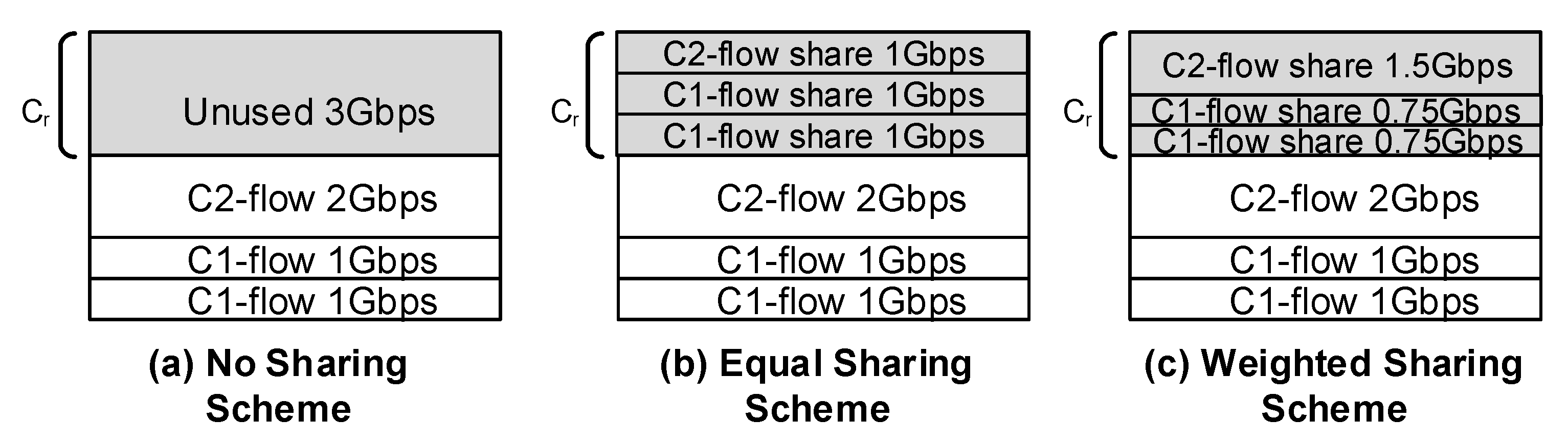
There are three possibilities to share the available residual capacity when $C_r>0$.

• No-Sharing ($NS$) Scheme: residual capacity $C_r$ is unused and it results in poor utilization of link capacity.
• Equal-Sharing ($ES$) Scheme: $C_r$ is shared equally among the active flows [35] and this scheme results are better than the no-sharing scheme.
• Weighted-Sharing ($WS$) Scheme: $C_r$ is distributed among active flow proportional to their class $MRR$ [17], and this scheme results in improved capacity utilization.

The sharing of residual capacity $C_r$ as per the above schemes is explained with an example in Figure 1 with $C=7$ Gbps, where the current state of the system is $(2,1)$ i.e., two active flows of class 1 and one active flow of class 2. We can easily compute that $C_r=3$ Gbps and the Figure 1 explains how it is shared among the active flows, as per the three schemes. In this study, experiments are conducted with an equal sharing scheme only.

5. Proposed Model

Markov chains are successfully used for performance evaluation of many different types of queuing systems. For given system parameters, we can easily find performance measures, like BP, link utilization, mean flow time, etc. These performance measures are helpful in system dimensioning and capacity planning for provisioning better QoS.

In a queuing system, the users are often classified into multiple classes, depending upon their service requirement and paying capacity. In such a multi-class environment, priority is often also assigned to each class signifying their level of importance. Various models are proposed for the analysis of multi-class priority queuing systems. These models are based on varying system parameters, as per the nature of the application, different arrival and services distribution, queuing mechanism, and priority handling (preemptive or non-preemptive, resume or restart). In the queuing system, lower class requests are blocked for two reasons: (a) blocked due to non-availability of capacity in the system and (b) ejected by the higher class. Aggregating these two types of probabilities, we will obtain the overall BP of the corresponding lower class. Most of the models proposed in the literature can help in finding the overall BP of the lower class. To the best of our knowledge, there is no such model that can provide us with insight into the two components of the BP of lower classes stated above.

The proposed model presents a novel and more intuitive approach for treating Markov chains to find the BP of individual classes. By using this novel approach, we can obtain the detailed BP of a particular class from which we can easily obtain blocking due to higher classes ejection and blocking due to system capacity. Typically, by solving Markov chains, we get the steady-state probability (SSP) vector $\pi$ from initial one-step transition probabilities, but, here, we are interested in finding steady transition probabilities (STP), i.e., long-term probabilities of the system taking each transition. Next, we explain this concept with a simple example.

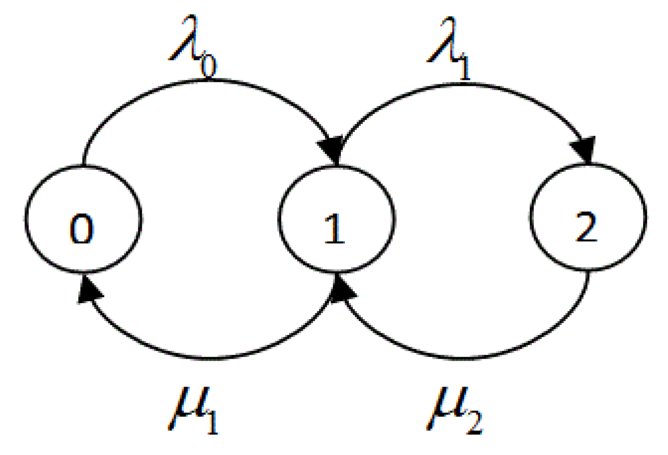
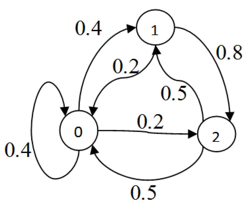
Consider a simple CTMC $(M/M/1/2)$ having three states, as shown in Figure 2, and the similarity rate matrix Q for this simple chain is given below

$$Q=\begin{array}{c}0\\ 1\\ 2\end{array}\stackrel{\begin{array}{cccccccccccc}0& & & & & 1& & & & & 2& \end{array}}{\begin{array}{}\left(\begin{array}{ccc}-{\lambda }_0& {\lambda }_0& 0\\ {\mu }_1& -({\lambda }_1+{\mu }_1)& {\lambda }_1\\ 0& {\mu }_2& -{\mu }_2\end{array}\right)\end{array}}$$

We can find one-step transition probability matrix P from the above matrix Q using the following formula

$$P=\frac{Q}{Max\left(q_{ii}\right)}+I$$

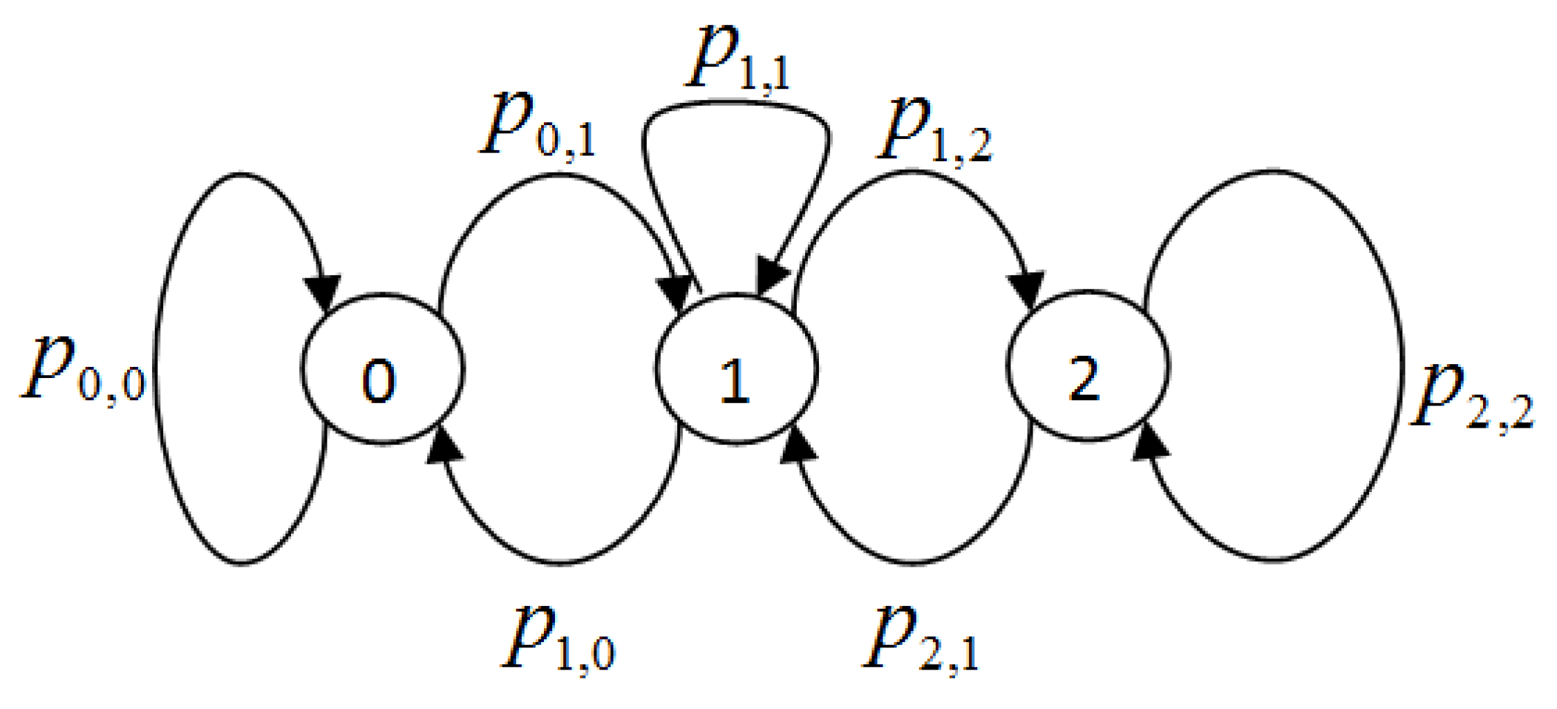
The Markov chain that is given in Figure 2 will look like that shown in Figure 3 in terms of one-step transition probabilities.

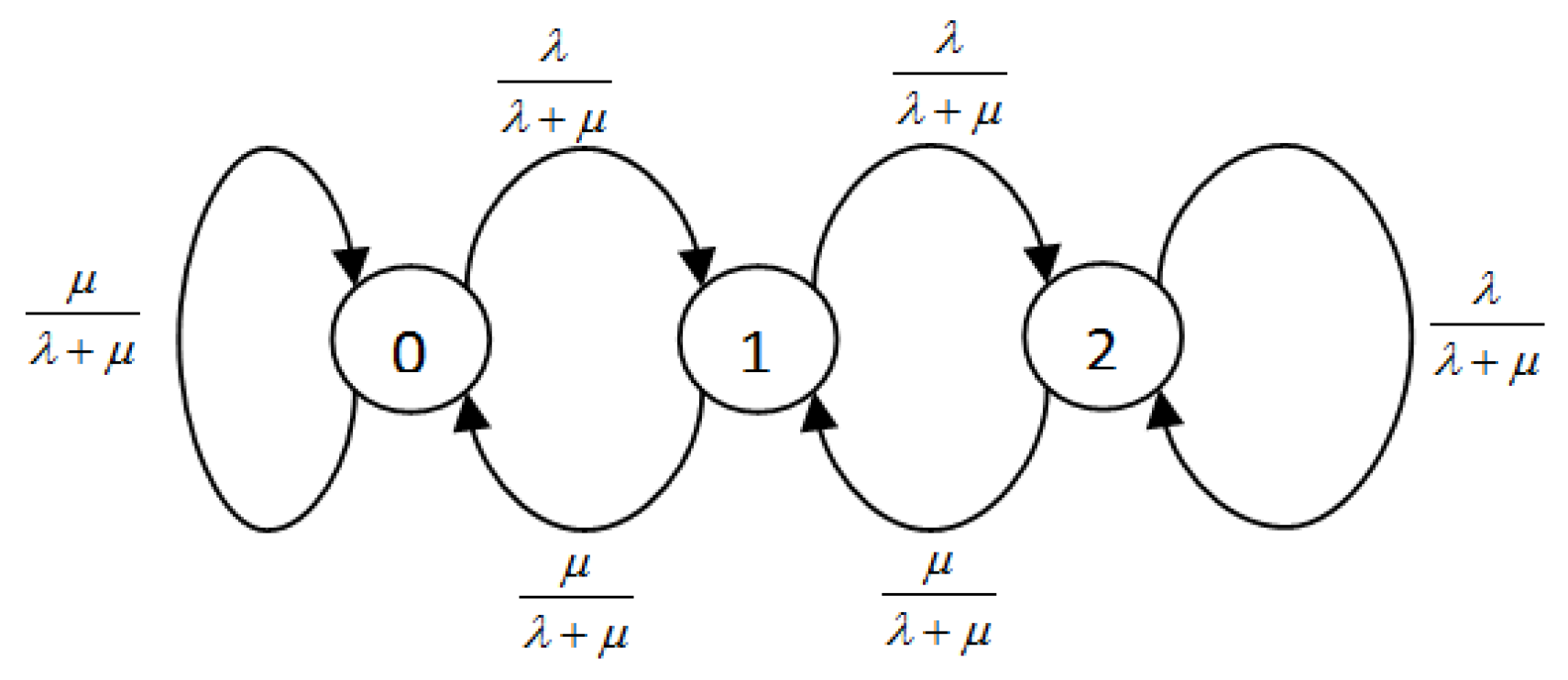
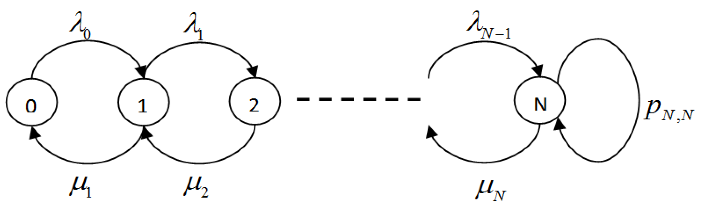
We are interested in finding steady transition probabilities (STP) $P_{i,j}\forall i,j$, i.e., the long term probability of the system taking each transition. In the next section, first, we will explain STP and how it can help provision the deep insight of blocking of the lower class in multi-service priority queuing system. Afterward, the concept of normalized arrival probabilities (NAP) is presented, i.e., another way of computing the blocking probability with proof of its correction while using a simple M/M/1/N queue as shown in Figure 4.

5.1. Steady Transition Probabilities (STP)

The concept of steady transition probabilities (STP) is just a detailed view of the Markov chain, and we can obtain steady-state probabilities from steady transition probabilities and vice versa. As stated earlier, STP is the long-term probabilities of the system taking each transition, and these can be calculated in two ways.

• Inverted Markov Chains
• Using SSP and one-step transition probability matrix P

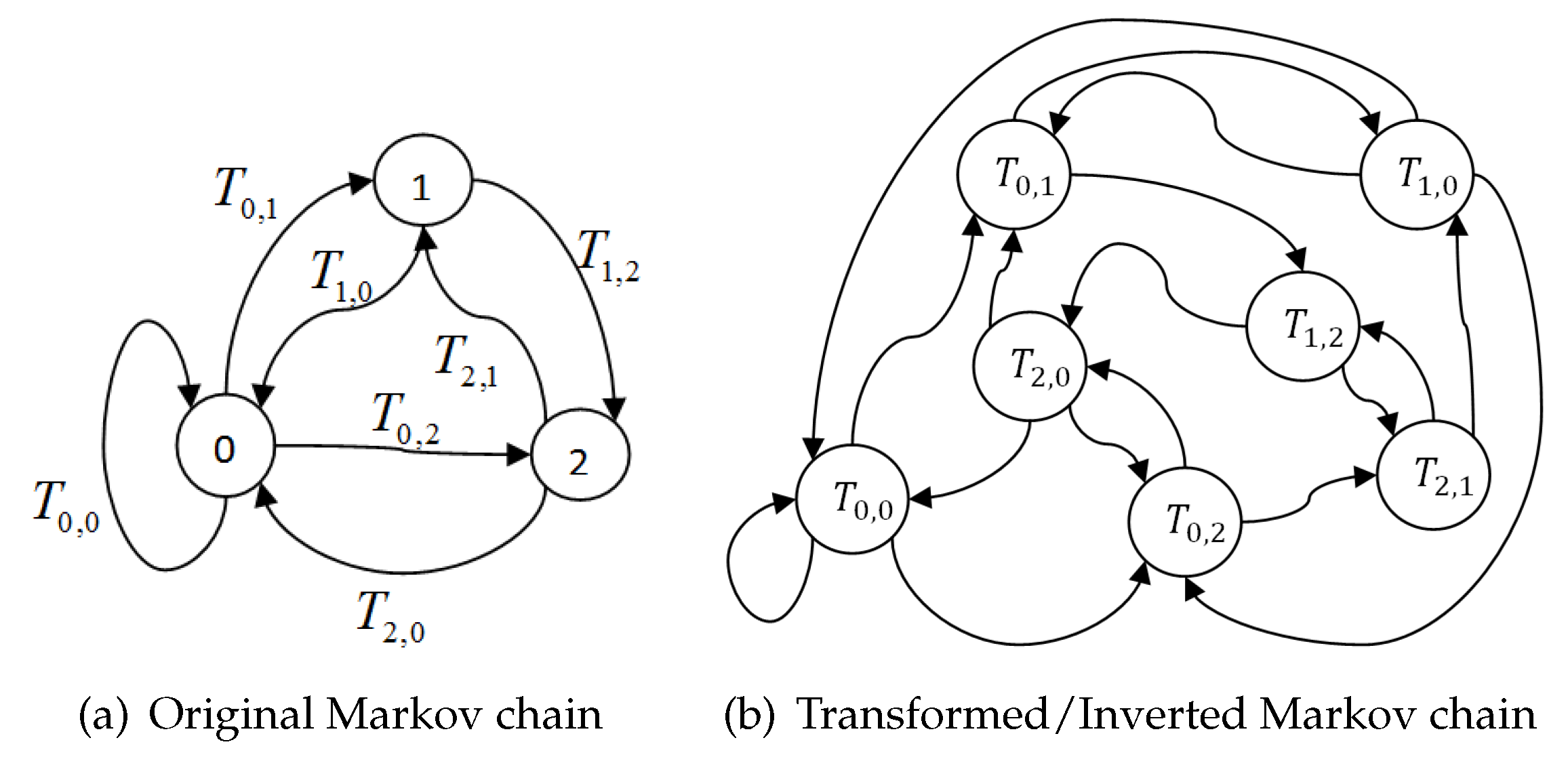
5.1.1. Inverted Markov Chains

By solving the Markov chain, we obtain steady-state probabilities, i.e., the long-term probability of the system being in every state. Using Inverted Markov Chains, we simply consider transitions as the states of the Markov chain and we need one step transition-to-transition probabilities in order to calculate STP. Consider the simple Markov chain with three states and inter-state transition probabilities, as given in Figure 5.

It is easy to get its one step probability matrix P, as below.

$$P=\begin{array}{c}0\\ 1\\ 2\end{array}\stackrel{\begin{array}{ccccc}0& & 1& & 2\end{array}}{\begin{array}{c}\left(\begin{array}{ccc}0.4& 0.4& 0.2\\ 0.2& 0& 0.8\\ 0.5& 0.5& 0\end{array}\right)\end{array}}$$

Once, we obtain the one step transition probability matrix P, the Iterative (Power) method [36] can be used to calculate the steady state probability vector $\pi$, as follows:

$${\pi }^{0}P={\pi }^1$$

$${\pi }^{1}P={\pi }^2$$

$$\cdots$$

$$li{m}_{n\to \infty }{\pi }^{n}P={\pi }^n$$

where ${\pi }^0$ is initial (random) probability distribution vector with condition ${\sum }_{i=1}^n{p}_i=1$. After solving for above chain (Figure 5), we get

$$\pi =\left(0.37036,0.30863,0.32103\right)$$

i.e.,

$$P\left(S_0\right)=0.37036$$

$$P\left(S_1\right)=0.30863$$

$$P\left(S_2\right)=0.32103$$

We now redraw Figure 5 by relabeling each transition as $T_{i,j}\forall i,j\in S$, as shown in Figure 6a, which shows the original Markov chain for sample M/M/1/2 queue along with the corresponding inverted Markov chain given in Figure 6b.

The one step transition to transition probability matrix is given below

$$P=\begin{array}{c}{T}_{0,1}\\ T_{0,2}\\ T_{0,0}\\ T_{1,2}\\ T_{1,0}\\ T_{2,0}\\ T_{2,1}\end{array}\stackrel{\begin{array}{ccccccc}{T}_{0,1}& T_{0,2}& T_{0,0}& T_{1,2}& T_{1,0}& T_{2,0}& T_{2,1}\end{array}}{\begin{array}{c}\left(\begin{array}{ccccccc}0& 0& 0& 0.8& 0.2& 0& 0\\ 0& 0& 0& 0& 0& 0.5& 0.5\\ 0.4& 0.2& 0.4& 0& 0& 0& 0\\ 0& 0& 0& 0& 0& 0.5& 0.5\\ 0.4& 0.2& 0.4& 0& 0& 0& 0\\ 0.4& 0.2& 0.4& 0& 0& 0& 0\\ 0& 0& 0& 0.8& 0.2& 0& 0\end{array}\right)\end{array}}$$

As it follows the Markov property, we can now find the steady transition probability vector $\pi$ in the same way and, after solving, we get

$$\pi =\left\{0.148148148,0.074074074,0.148148148,0.24691358,0.061728395,0.160493827,0.160493827\right\}$$

i.e.,

$$P\left(T_{0,1}\right)=0.148148148$$

$$P\left(T_{0,2}\right)=0.074074074$$

$$P\left(T_{0,0}\right)=0.148148148$$

$$P\left(T_{1,2}\right)=0.24691358$$

$$P\left(T_{1,0}\right)=0.061728395$$

$$P\left(T_{2,0}\right)=0.160493827$$

$$P\left(T_{2,1}\right)=0.160493827$$

We can easily see that for any state s

$$\sum _{\forall i}P\left(T_{i,s}\right)=\sum _{\forall j}P\left(T_{s,j}\right)=P\left(s\right)$$

i.e., the sum of all transition probabilities into state s is equal to the sum of transition probabilities out of state s and that is equal to the probability of being in state s e.g., for $S_1$, we can easily see that,

$$P\left(T_{0,1}\right)+P\left(T_{2,1}\right)=P\left(T_{1,2}\right)+P\left(T_{1,0}\right)=P\left(S_1\right)$$

$$0.148148148+0.160493827=0.24691358+0.061728395=0.30863$$

$$0.308641975=0.308641975=0.30863$$

The same can be observed for all other states. This shows that STP gives us a more detailed view of the system long term probabilities.

5.1.2. Alternative Approach Based on $SSP$ and P

From the previous results, we can easily deduce that

$$P\left(T_{i,j}\right)=P\left(S_i\right).p_{i,j}$$

(3)

For example,

$$P\left(T_{0,1}\right)=P\left(S_0\right).p_{0,1}$$

$$P\left(T_{0,2}\right)=P\left(S_0\right).p_{0,2}$$

$$P\left(T_{0,0}\right)=P\left(S_0\right).p_{0,0}$$

⇒

$$P\left(T_{0,1}\right)+P\left(T_{0,2}\right)+P\left(T_{0,0}\right)=P\left(S_0\right).(p_{0,0}+p_{0,1}+p_{0,2})$$

As $p_{1,1}+p_{1,2}+p_{1,3}=1$ therefore we get

$$P\left(T_{0,1}\right)+P\left(T_{0,2}\right)+P\left(T_{0,0}\right)=P\left(S_0\right)$$

This method gives us a simple way to calculate STP, and this is more convenient in terms of computation as for large size CTMC, the size of one-step transition-to-transition probability matrix will grow enormously and it will require greater computations. In other words, we can simply calculate the steady transition probability of any transition $T_{i,j}$ using Equation (3).

5.2. Normalized Arrival Probabilities ($NAP$)

STP gives us the long term probabilities of the system taking any transition. Mainly, we have two types of transitions in CTMC, i.e., arrivals and departures. For capacity planning, we are often interested in system BP, which is only related to arrivals only. Let T be the set of all transition probabilities, then we can express it as

$$T=T_A+T_D$$

where $T_A$ and $T_D$ are the set of arrival and departure probabilities, respectively.

Here, we are only interested in arrival probabilities and let the summation of all arrival probabilities be D, i.e.,

$$\sum P\left(T_{i,j}\right)=D\forall T_{i,j}\in T_A$$

It can be observed that, for constant arrival and service rates,

$$\sum P\left(T_{i,j}\right)=\frac{\lambda }{\lambda +\mu }$$

We divide each arrival transition by D to obtain the Normalized Arrival Probability (NAP), i.e.,

$$\overline{P}\left(T_{i,j}\right)=\frac{P\left(T_{i,j}\right)}{D}\Rightarrow \sum \overline{P}\left(T_{i,j}\right)=1$$

This $NAP$ gives us the distribution of arrivals, e.g., if the total no. of arrival into the system is A, then the arrival count along with each arrival transition $AC\left(T_{i,j}\right)$ is given by

$$AC\left(T_{i,j}\right)=\overline{P}\left(T_{i,j}\right)\times A$$

Thus, we obtain the approximate no. of arrivals on each arrival transition.

5.3. Using NAP to compute BP of $M/M/1/N$ queuing system

In this section, we will show how to use NAP to find the BP of the system. We will also prove that its result is the same as the BP calculated using traditional SSP. For instance, see Figure 4, in which the blocking probability of the system is the probability of the system being in state N i.e., $P\left(N\right)$, and the same result can be obtained using $NAP$.

This is very intuitive to choose $\overline{P}\left(T_{N,N}\right)$ only because all other arrivals are accommodated by the system and they cause a transition from one state to another. $T_{N,N}$ is the only looping transition in $M/M/1/N$, i.e., arrivals along with this transition cause no change in the system’s state (loopback). In other words, all of the arrivals along $T_{N,N}$ are blocked by the system. That is why we say that the BP of the system in NAP is the looping transitions in the case of $M/M/1/N$ i.e., $\overline{P}\left(T_{N,N}\right)$ and this is more intuitive. Next, we will try to prove the following

$$P\left(N\right)=\overline{P}\left(T_{N,N}\right)$$

For sake of illustration, we limit our queue size to $N=2$ i.e., $M/M/1/2$ with arrival $\lambda$ and service rate $\mu$, as shown in Figure 2.

Similarity, the Rate Matrix Q of above $M/M/1/2$ queue is given below.

$$Q=\begin{array}{c}0\\ 1\\ 2\end{array}\stackrel{\begin{array}{ccccccccc}0& & & & 1& & & & 2\end{array}}{\begin{array}{c}\left(\begin{array}{ccc}-\lambda & \lambda & 0\\ \mu & -(\lambda +\mu )& \lambda \\ 0& \mu & -\mu \end{array}\right)\end{array}}$$

We can find steady-state probabilities of this simple $M/M/1/2$ by solving the following birth–death equation.

$$\lambda P_0=\mu P_1\Rightarrow P_1=\frac{\lambda }{\mu }{P}_0$$

$$P_2=\frac{{\lambda }^2}{{\mu }^2}{P}_0$$

we know that

$$P_0+P_1+P_2=1$$

$$P_0+\frac{\lambda }{\mu }{P}_0+\frac{{\lambda }^2}{{\mu }^2}{P}_0=1$$

$$P_0=\frac{1}{1+\frac{\lambda }{\mu }+\frac{{\lambda }^2}{{\mu }^2}}$$

$$P_0=\frac{{\mu }^2}{{\lambda }^2+\lambda \mu +{\mu }^2}$$

$$P_1=\frac{\lambda }{\mu }{P}_0$$

$$P_1=\frac{\lambda }{\mu }\frac{{\mu }^2}{{\lambda }^2+\lambda \mu +{\mu }^2}=\frac{\lambda \mu }{{\lambda }^2+\lambda \mu +{\mu }^2}$$

and the BP of the system is $P_2$

$$P_2=\frac{{\lambda }^2}{{\mu }^2}{P}_0$$

$$P_2=\frac{{\lambda }^2}{{\mu }^2}\frac{{\mu }^2}{{\lambda }^2+\lambda \mu +{\mu }^2}=\frac{{\lambda }^2}{{\lambda }^2+\lambda \mu +{\mu }^2}$$

We now try to find the same result using NAP, which is calculated by using SSP and one-step transition probabilities. To obtain one-step transition probabilities, we use the following formula

$$P=\frac{Q}{Max\left(q_{ii}\right)}+I$$

Hence,

$$P=\begin{array}{c}0\\ 1\\ 2\end{array}\stackrel{\begin{array}{ccccccc}0& & & 1& & & 2\end{array}}{\begin{array}{c}\left(\begin{array}{ccc}\frac{\mu }{\lambda +\mu }& \frac{\lambda }{\lambda +\mu }& 0\\ \frac{\mu }{\lambda +\mu }& 0& \frac{\lambda }{\lambda +\mu }\\ 0& \frac{\mu }{\lambda +\mu }& \frac{\lambda }{\lambda +\mu }\end{array}\right)\end{array}}$$

Redraw Figure 2 using one-step transition probabilities, we get the picture that is shown in Figure 7 (transition probability with zero value are ignored)

We can see that, among these six transitions, three are arrivals, i.e., $T_{0,1},T_{1,2},T_{2,2}$. We can find $NAP$, as below

$$P\left(T_{0,1}\right)=P\left(0\right).p_{0,1}=\frac{{\mu }^2}{{\lambda }^2+\lambda \mu +{\mu }^2}\frac{\lambda }{\lambda +\mu }=\frac{\lambda {\mu }^2}{z}$$

where

$$z=(\lambda +\mu )({\lambda }^2+\lambda \mu +{\mu }^2)$$

Similarly,

$$P\left(T_{1,2}\right)=P\left(1\right).p_{1,2}=\frac{\lambda \mu }{{\lambda }^2+\lambda \mu +{\mu }^2}\frac{\lambda }{\lambda +\mu }$$

$$=\frac{{\lambda }^2\mu }{z}$$

$$P\left(T_{2,2}\right)=P\left(2\right).p_{2,2}=\frac{{\lambda }^2}{{\lambda }^2+\lambda \mu +{\mu }^2}\frac{\lambda }{\lambda +\mu }$$

$$=\frac{{\lambda }^3}{z}$$

We can now compute that normalized arrival probability $\overline{P}\left(T_{2,2}\right)$, as below

$$\overline{P}\left(T_{2,2}\right)=\frac{\frac{{\lambda }^3}{z}}{\frac{\lambda {\mu }^2}{z}+\frac{{\lambda }^2\mu }{z}+\frac{{\lambda }^3}{z}}$$

$$=\frac{{\lambda }^2}{{\lambda }^2+\lambda \mu +{\mu }^2}$$

Thus, we have proved that

$$P\left(2\right)=\overline{P}\left(T_{2,2}\right)$$

This can be easily be extended to $M/M/N/N$. Moreover, for constant arrival rate $\lambda$ and service rate $\mu$, we can easily find out that sum of all services transitions

$$\sum P\left(T_{i,j}\right)=\frac{\mu }{\lambda +\mu }\forall T_{i,j}\in T_D$$

and the probability of the system being in an idle state is as below

$$\overline{P}\left(T_{0,0}\right)=P\left(0\right)=\frac{{\mu }^2}{{\lambda }^2+\lambda \mu +{\mu }^2}$$

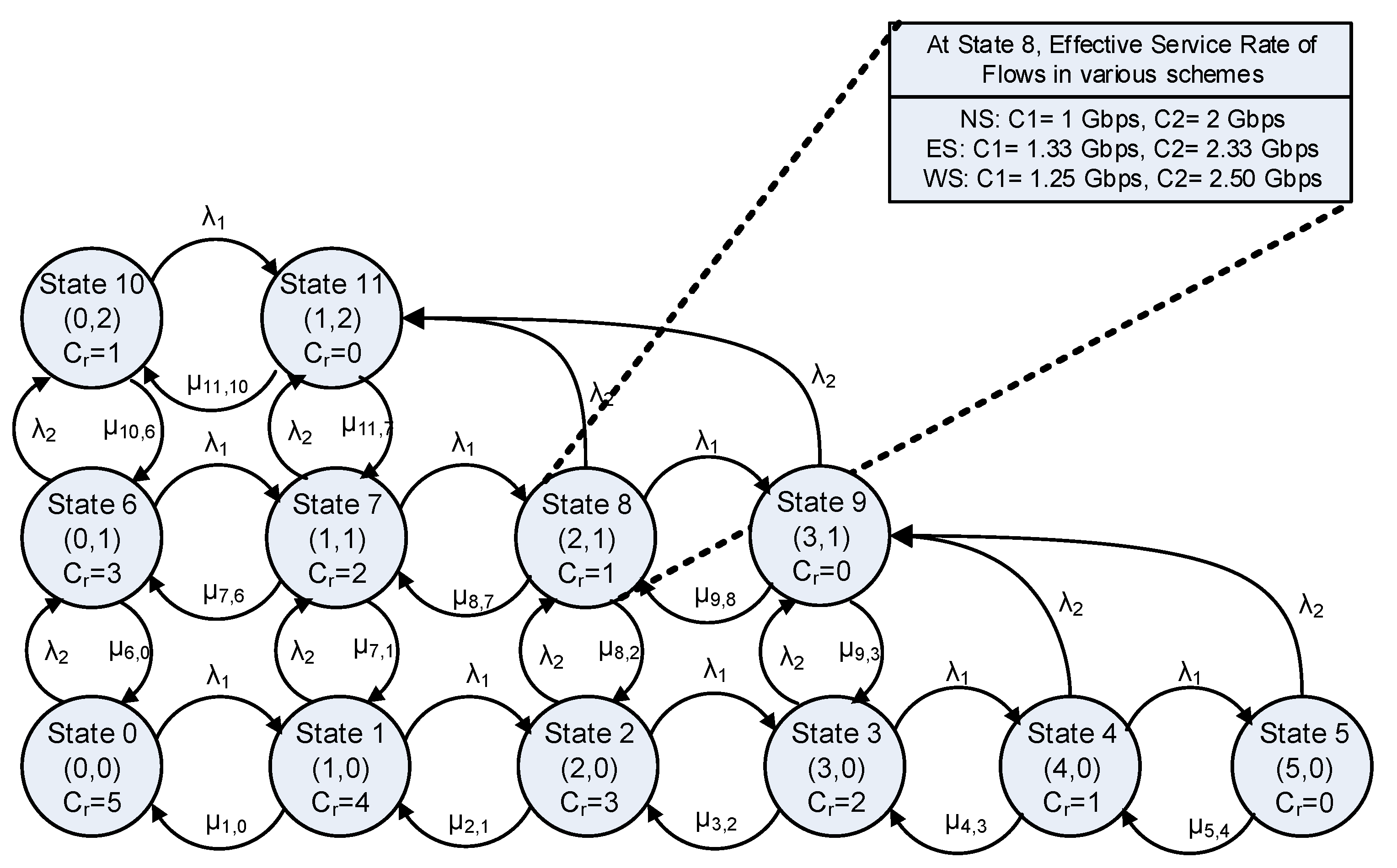
5.4. Model Implementation

We have modeled the bottleneck link of the network as a constant capacity C server. Arrivals of multi-class requests are assumed to follow Poisson and the services are exponentially distributed with mean volume V. Thus, the system is modeled as a multi-dimensional Continuous Time Markov Chain (CTMC), as shown in Figure 8. Given the system is in state $S_i$, then the arrival of $c^{th}$ request will result in a transition to state $S_j$ and completion of a $c^{th}$ class job will result in a transition to state $S_k$.

$$S_i=(N_1,N_2,\dots ,N_c,\dots ,N_R)$$

$$S_j=(N_1,N_2,\dots ,N_c+1,\dots ,N_R)$$

$$S_k=(N_1,N_2,\dots ,N_c-1,\dots ,N_R)$$

As arrival of all classes is equally likely and they are generated using Poisson distribution, therefore the transition rate from state $S_i$ to $S_j$ uponthe arrival of a $c^{th}$ class request will become:

$${\lambda }_{i,j}={\lambda }_c$$

(4)

Upon the completion of a request of class c, the system will make a transition from state i to state k. As in this study, the experiments are only conducted with an equal sharing scheme, and the service rate for this scheme is calculated, as follows:

$${\mu }_{i,k}=\left\{\begin{array}{cc}\frac{N_c}{V}\left(MR{R}_c+\frac{C_r}{{\sum }_{i=1}^R{N}_i}\right)& for{N}_c>0\\ 0& otherwise\end{array}\right\}$$

(5)

where V is the mean size of the requests and $N_c$ are the total number of active flows of class c in-state i.

Figure 8 presents a sample CTMC for two classes with $C=5$ Gbps. Class 2 jobs have preemption priority over class 1. It can be noted that, un states 4 and 5, there is no room for newly arriving requests of class 2, therefore transition is made to state 9, which results in the ejection of 1 and 2 requests of class 1, respectively. Likewise, the transition from states 8 and 9 to state 11 also results in the ejection of class 1 jobs.

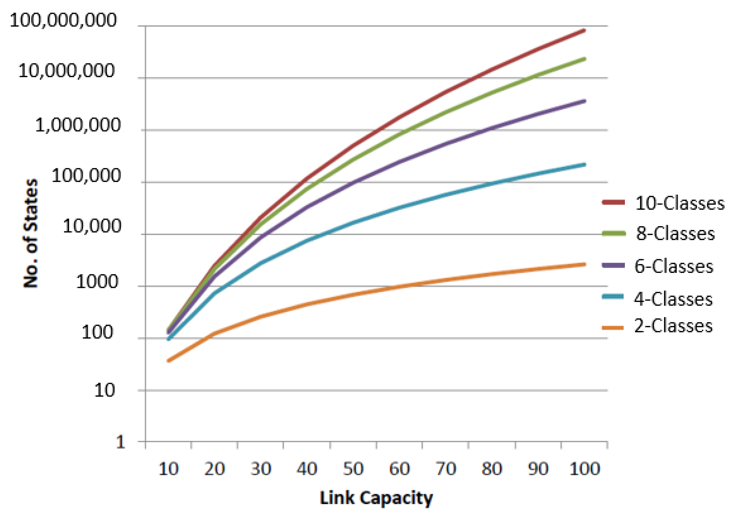
The total number of states in the CTMC grows exponentially with the increase in the link capacity C and total number of classes, as shown in Figure 9. A state S in CTMC is valid if:

$$\sum _{i=1}^R\left(N_i\times MR{R}_i\right)\le C$$

where $N_i$ is the total number of active flows of $i^{th}$ class having a minimum flow rate $MR{R}_i$.

After generating all of the possible states and corresponding transition probabilities, CTMC is solved using the iterative method, and we get steady-state probability vector $\pi$ of the system, which is then used to compute blocking probabilities of the overall system and individual classes and subsequent performance analysis.

5.4.1. Computation of BP

The blocking probabilities of the overall system and individual classes are computed while using the steady-state probability vector $\pi$. To compute $BP$ of class x, set $S_{B_c}$ of all those states in CTMC is required where a new request of class x cannot be accommodated. Thus, the blocking probability of high priority class x can be computed, as below:

$$B{P}_x=\sum _{\forall s\in S_{B_x}}{p}_s$$

where $p_s$ is the long term probability of the system being in state s.

The blocking probability of lower priority class y can be computed, as below:

$$B{P}_y=\sum _{\forall s\in S_{B_{y1}}}{p}_s+\sum _{\forall t\in S_{T_A}}\overline{P}\left(T_{i,j}\right)\times MR{R}_x$$

where $S_{T_A}$ is a subset of normalized arrival probabilities, which results in the ejection of lower-class requests.

Blocking probability of the overall system can be computed as below:

$$BP=\left[\sum _{c=1}^R\left(B{P}_c\right)\right]\times \frac{1}{\lambda }$$

(6)

5.4.2. Computation of Link Utilization

Percentage link utilization $C_{util}$ of the system having link capacity C is computed from state probability vector $\pi$, as follows:

$$C_{util}=\frac{{\sum }_{\forall s\in \Theta }{p}_s\times (C-C_r\left(s\right))}{C}\times 100$$

where $C_r\left(s\right)$ is the link residual capacity in state s.

6. Performance Evaluation

The objectives of performance evaluation are:

• To validate the proposed model results.
• To highlight effect on overall system blocking probability, due to preemptive priority as compared to the non-preemptive model.
• To conduct a class-wise comparative analysis of blocking probabilities for preemptive and non-preemptive models.
• To present a detailed analysis of lower-class blocking probabilities.
• To perform analysis of link capacity utilization with varying traffic intensities.

The proposed model validation is conducted through simulation using an ad-hoc simulator that was developed in Microsoft Visual Studio 2017 using Visual Basic .NET (VB.NET). The simulation model considers an ideal network environment and it does not capture the network/packet-level details such as losses and overheads. In every simulation experiment, 100,000 requests/flows are generated using Poisson distribution. The flow volumes are exponentially distributed with mean a value of V.

Table 1. Configuration setup for simulation and model.

S. No.	Parameter/Variable	Value/Range
		Simulation	Model
1	Number of classes	2
2	Arrival rate	0.25
3	Link capacity	20, 30, 40 Gbps
4	Traffic intensity	0.5–2.0 (step 0.1)
5	Total number of requests	100,000		NA
6	Size of individual flow	Exp. distributed in range 40–160 (step 8) for $C=20$ 60–240 (step 12) for $C=30$ 80–320 (step 16) for $C=40$		NA

presents the summary of configuration for different parameters that are related to models and simulations. The reported results are the average values for 10 different simulation runs for each experimental setup.

For the sake of simplicity and without losing any generality, the arrival rate of all classes is considered to be the same, i.e.,

$${\lambda }_c=\frac{\lambda }{R}$$

where R is the total number of classes and $\lambda$ is the arrival rate of all requests.

We know that traffic intensity $\rho$ can be computed, as below:

$$\rho =\frac{\lambda \times V}{C}$$

For a given/desired traffic intensity, the mean flow size V can be obtained as

$$V=\frac{\rho \times C}{\lambda }$$

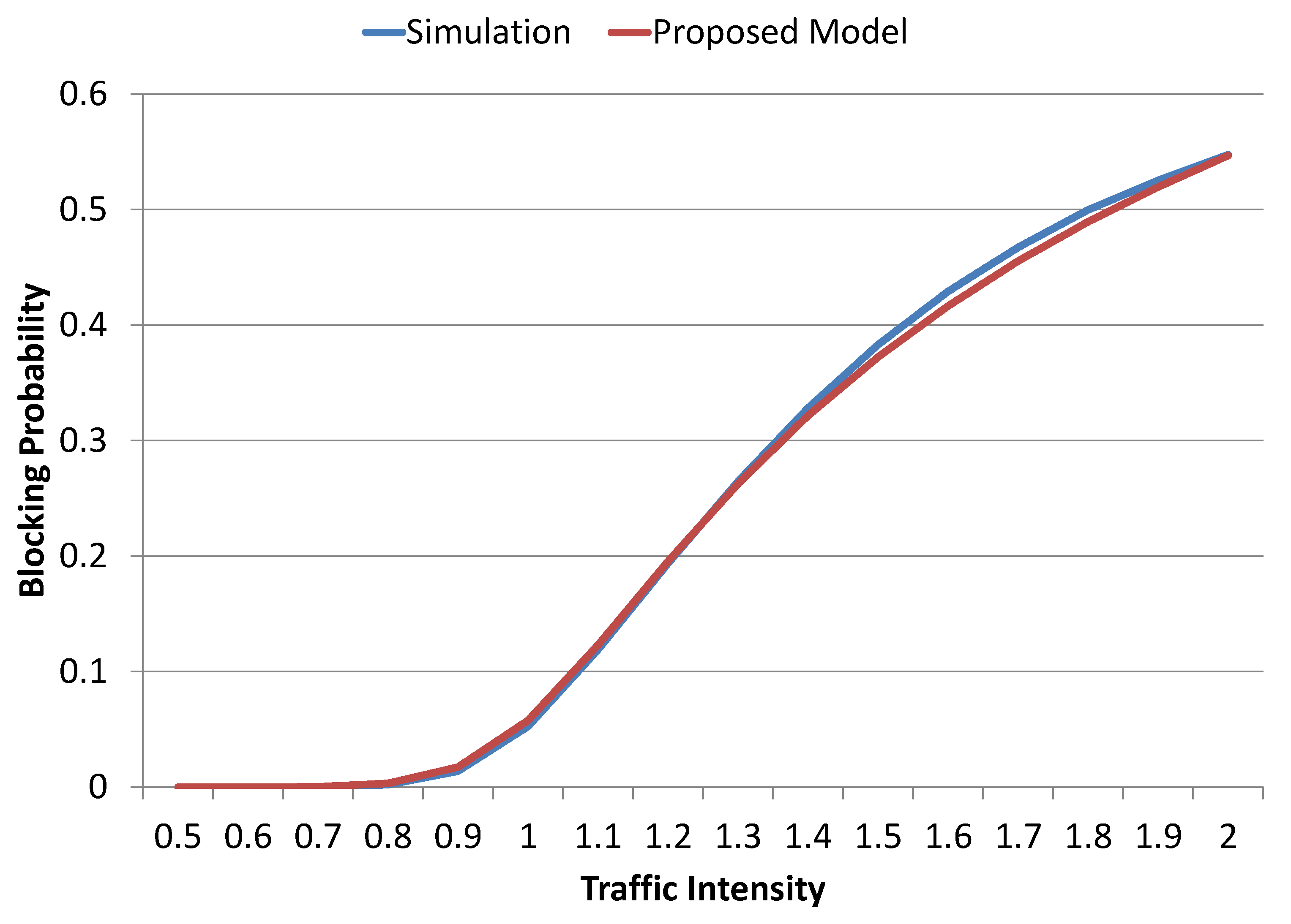
Figure 10 shows the blocking probabilities that were calculated for various traffic intensities using analytical model and simulation while considering the link capacity of $C=30$ Gbps. Model and simulation results are both nicely aligned for all traffic intensities varying from 0.5 to 2.0. These results clearly show that the simulations validate the model. For traffic intensities that are below 1.0, the overall system blocking probability is very low (acceptable). However, a significant increase in the blocking probabilities can be observed as traffic intensity approaches 2.0, where more than $50\%$ of requests are blocked by the system. Furthermore, these results also confirmed that the system blocking probability is not linearly increasing with the increase in traffic intensity.

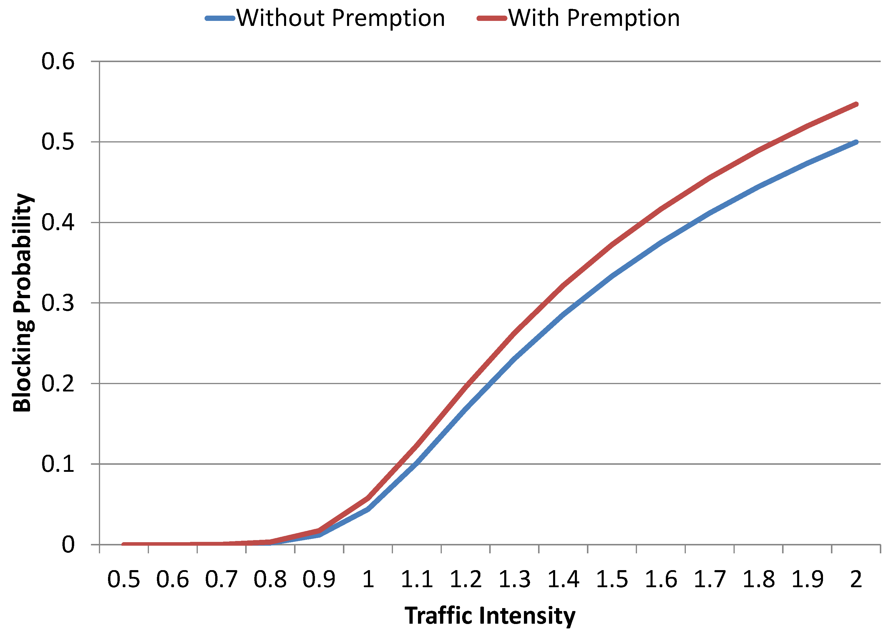
Next, we study the effect on the overall system blocking probability due to preemptive priority as compared to the non-preemptive model [17]. Figure 11 presents the comparative analysis of blocking probabilities for preemptive and non-preemptive models results with $C=30$ Gbps. For traffic intensities that are below 1.0, there is no significant difference in blocking probabilities of the two models, and this is due to the underutilization of link capacity. However, a gradual increase in difference among the blocking probabilities of the two models can be observed as traffic intensity approaches 2.0 where approx. $50\%$ and $55\%$ of requests are blocked by the system in case of the non-preemptive and preemptive model, respectively. These results show that the preemptive model results in less than a $5\%$ (absolute) increase in the system overall blocking probability when compared to its counterpart non-preemptive model.

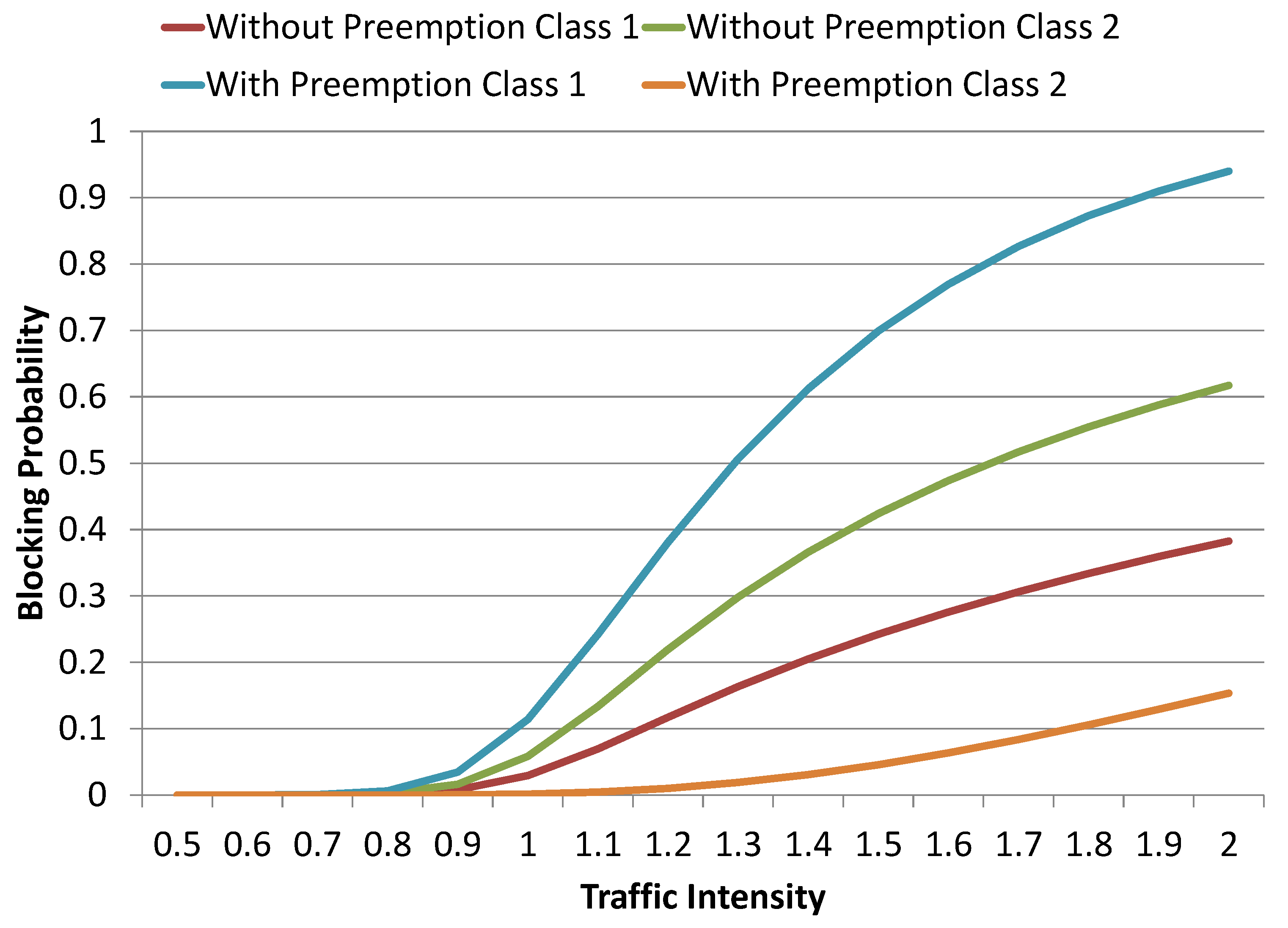
An increase in the system overall blocking probability by the preemptive model is not particularly significant, i.e., less than $5\%$ (absolute) when compared to its counterpart non-preemptive model. However, a detailed investigation of individual class probabilities revealed a significant increase in the lower-class (class 1) probabilities, as shown in Figure 12. Once again, for traffic intensities that are below 1.0, the difference in individual class blocking probabilities of the two models is very low, which is due to the underutilization of link capacity. However, a significant increase in difference among the individual class blocking probabilities of the two models can be observed with an increase in traffic intensity. In the case of the non-preemptive model, for a traffic intensity of 2.0, the blocking probabilities of class 1 and class 2 are $38\%$ and $61\%$, respectively. When both of the classes are treated equally by the system, then class requests are experiencing high blocking probability due to their high QoS requirement i.e., $2MRR$. Whereas, in the case of the preemptive model, the same blocking probabilities changed to $94\%$ and $15\%$, for class 1 and class 2, respectively. The significantly high blocking probabilities of class 1 ($94\%$) is due to two reasons: (a) being blocked by the system due to unavailability of required QoS ($1MRR$) as a result of high utilization of system capacity and (b) ejected by the system to make room for high priority jobs. The whole link capacity is available for class 2 requests, as if class 1 requests do not exist (virtually) and, therefore, the blocking probability of class 2 is reduced from $61\%$ to $15\%$, for traffic intensity of 2.0.

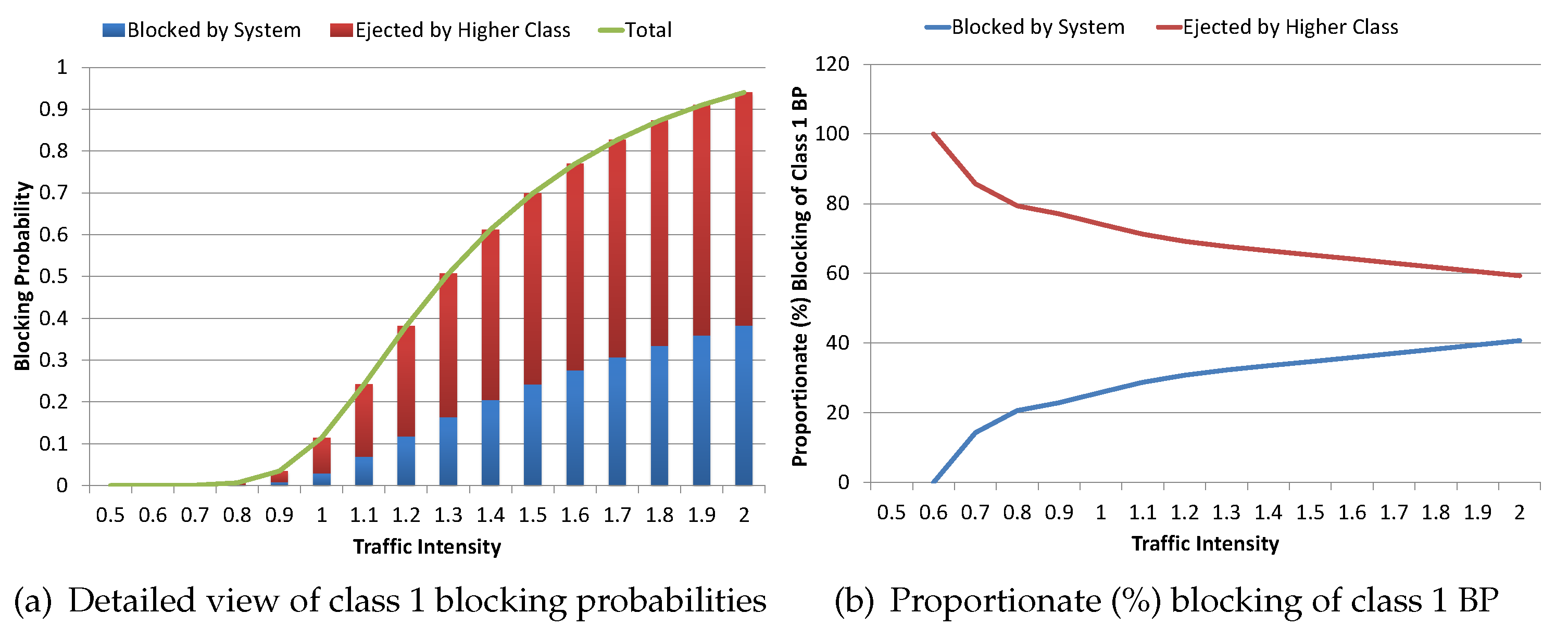
Class-wise comparative analysis of blocking probabilities, as given in Figure 12, indicate a significant increase ($147.43\%$) in the blocking probabilities of class 1 for the preemptive model when compared to the non-preemptive model. This is due to two reasons: (a) being blocked by the system due to unavailability of required QoS (b) ejected by the system to make room for high-priority jobs. Figure 13 shows the detailed analysis of blocking probabilities components for class 1 while using preemptive model results with $C=30$ Gbps, No. of classes $R=2$ and $MR{R}_c=cGbps\forall c\in \left\{1,\dots ,R\right\}$. Figure 13a provided detailed insight regarding class 1 blocking probabilities, along with the contribution of each component, in total, the blocking probabilities. We can observe that a major portion of the class 1 requests are blocked due to ejection by the arrival of higher class jobs as compared to blocking by the system due to the unavailability of the required QoS. This is due to the relatively higher QoS requirement of class 2 jobs i.e., having $MRR=2$ Gbps. In other words, when the residual capacity is zero, the arrival of the class 2 job will cause an ejection of two requests (in progress) of class 1 if available. This is also evident from Figure 13b, which provides proportionate (%) blocking of class 1 blocking probability. For lower traffic intensities, a relatively low percentage of class 1 requests are blocked by the system as compared to the ones ejected by higher classes. For instance, with a traffic intensity of 1.0, around $10\%$ requests of class 1 are blocked and, out of these $10\%$ blocked requests, around $25\%$ are blocked by the system, and $75\%$ are ejected due to the arrival of higher class requests. Whereas, with a traffic intensity of 2.0, a total of around $94\%$ requests of class 1 are blocked and, out of these $94\%$ blocked requests, around $40\%$ are blocked by the system whereas $60\%$ are ejected due to the arrival of higher class requests. In other words, more requests of class 1 are blocked by the system with an increase in traffic intensity due to high link utilization.

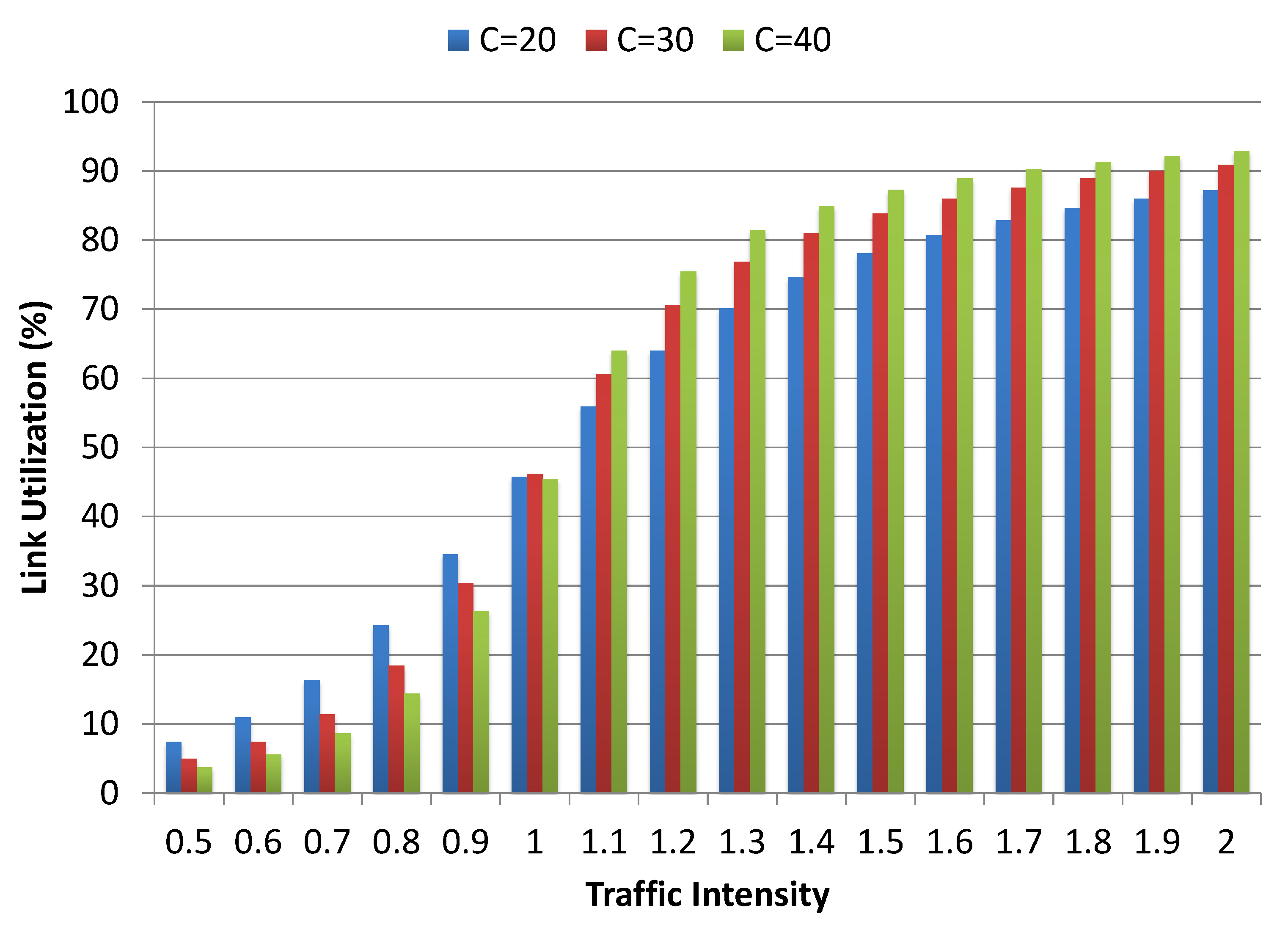
Figure 14 shows the percentage link capacity utilization by proposed model with varying traffic intensities for $C=20,30,40$ Gbps. For traffic intensities that are below 1.0, the link capacity utilization is below $35\%$, i.e., significant link capacity is available most of the time, which is the main reason for having significantly low blocking probabilities for traffic intensities that are below 1.0. A gradual increase in the link capacity utilization can be observed as the traffic intensity increases beyond 1.0 up to 1.5, but, afterward, there is no significant improvement in link capacity utilization. This shows that, as we approach towards the maximum achievable link utilization, an increase in traffic intensity contributes less in maximizing link utilization and, in contrast, it results in a drastic increase in the system blocking probability, which is evident from earlier results. Figure 14 also shows that, with an increase in traffic intensity, link utilization exhibits a converse behavior with an increase in the link capacities. For instance, with lower link capacity ($C=20$ Gbps), link utilization grows faster in the early stages and gets slower towards the end to reach the maximum. Conversely, with higher link capacity ($C=40$ Gbps), the growth in link utilization is slower in the beginning and it gets faster towards the end to reach the maximum.

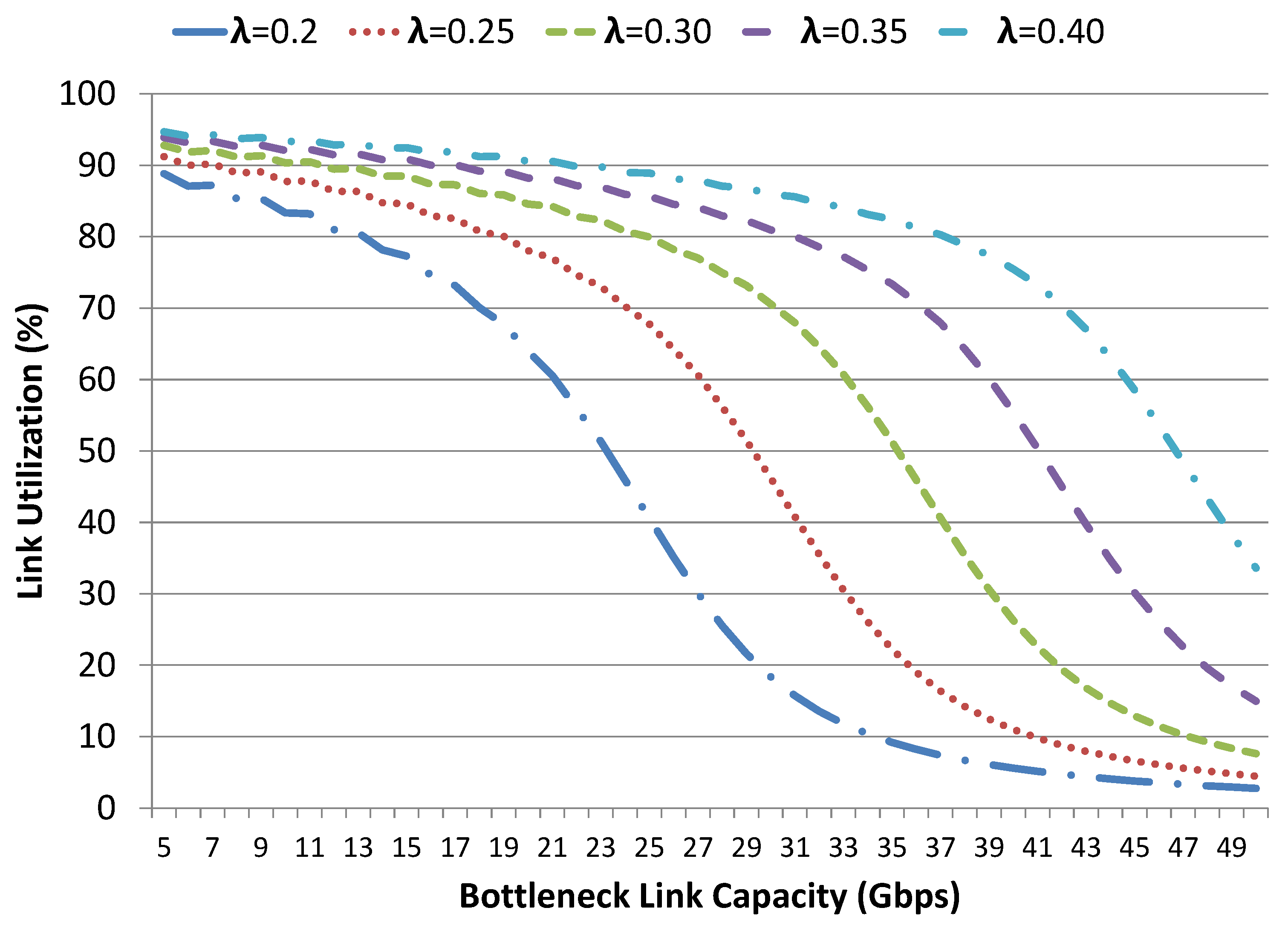
In order to further illustrate the bottleneck link capacity utilization, we have conducted another set of experiments with varying requests arrival rate $\lambda =\{0.20,0.25,0.30,0.35,0.40\}$ having a mean volume size of 120 Gbps and the results are shown in Figure 15. It is evident from the results that, for low bottleneck link capacities, the link utilization is very high, i.e., around 90% for all arrival rates. As we increase the bottleneck link capacity, a gradual decrease in link utilization can be observed. For lower arrival rate $\lambda =0.20$, the decrease in link utilization is faster when compared to the results of a higher arrival rate $\lambda =0.40$. For instance, for $\lambda =0.20$, when the bottleneck link capacity C is increased from 20 Gbps to 40 Gbps, the link utilization is reduced from $64\%$ to $5.57\%$. Whereas, for $\lambda =0.40$, when the bottleneck link capacity C is increased from 20 Gbps to 40 Gbps, the link utilization is reduced from $90.55\%$ to $75.46\%$.

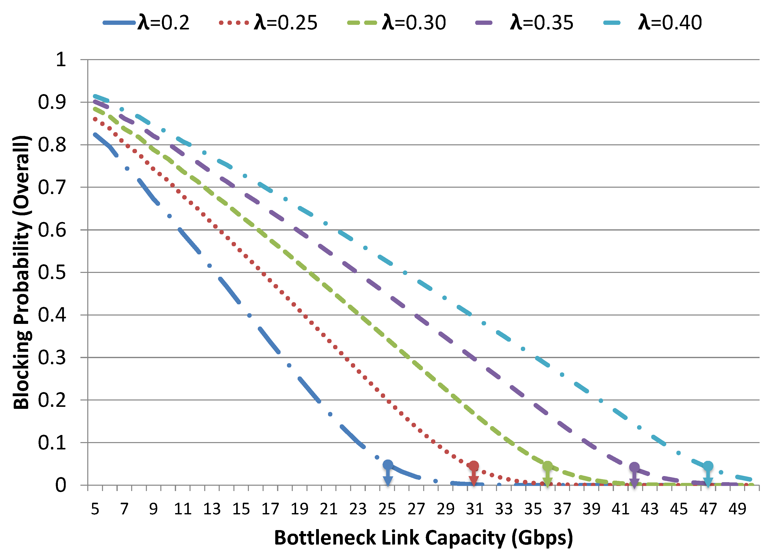
Algorithm 1 can be used for network capacity planning in order to compute optimal bottleneck link capacity for a given traffic intensity and requests an arrival rate, such that the overall network blocking probability remains within a certain acceptable range, i.e., $\left[B{P}_{lim}-\alpha ,B{P}_{lim}+\alpha \right]$.

The experiments are conducted for a certain case study with varying requests for arrival rate $\lambda =\{0.20,0.25,0.30,0.35,0.40\}$ having mean volume size of 120 Gbps. Here, we are interested in finding the optimal bottleneck link capacity, such that the overall network blocking probability remains with a certain acceptable range i.e., $B{P}_{lim}=0.05$ with $\alpha =0.002$. There are two classes of user requests and $MRR$ for class-1 and class-1 requests are 1 Gbps and 2 Gbps, respectively. Furthermore, class-2 requests have preemptive priority over class-1. Figure 16 provides the proposed model results for the aforementioned case study. The results show that the overall blocking probability of the system gets decreased with the gradual increase in bottleneck link capacity and, finally, we obtain different optimal bottleneck link capacity for each arrival rate, as indicated in Figure 16. With the increase in the arrival rate of incoming requests, we need to increase the bottleneck link capacity in order to have the overall blocking probability of the system below the desired range. For instance, the optimal bottleneck link capacity is 31 Gbps for the request arrival rate $\lambda =0.25$ in order to have the overall blocking probability around $0.05$. Whereas, for request arrival rate $\lambda =0.40$, the optimal bottleneck link capacity results in 47 Gbps. This is just an example to illustrate the utility of the proposed model in the capacity planning of a network with given traffic conditions.

Algorithm 1 Network Capacity Planning

Require:$V,\lambda ,C_{max},B{P}_{lim},\alpha$

Ensure:$C_{opt}$

$C_{min}\leftarrow 0$

$BP\leftarrow 1$

$flag\leftarrow false$

while $flag\ne true$ do

$C_{cur}\leftarrow (C_{min}+C_{max})/2$

Generate system states S for $C_{cur}$

Compute states transition probabilities for S using $\lambda$ and Equation (5)

Compute states-state probability vector $\pi$

Update $BP$ using Equation (6)

if $BP\in \left[B{P}_{lim}-\alpha ,B{P}_{lim}+\alpha \right]$ then

$C_{opt}\leftarrow C_{cur}$

$flag\leftarrow true$

end if

if $BP<B{P}_{lim}$ then

$C_{max}\leftarrow C_{cur}$

else

$C_{min}\leftarrow C_{cur}$

end if

end while

return $C_{opt}$

7. Conclusions and Future Work

In this paper, we have presented a novel analytical model for a multi-service queue with deadline and priority constraints. The model is validated through simulations of bulk data transfers using the equal sharing scheme of residual capacity. The proposed model results in less than a $5\%$ increase of the system overall blocking probability when compared to its counterpart non-preemptive model. Detailed class-wise comparative analysis of blocking probabilities revealed that a significant increase ($147.43\%$) in the lower class (class 1) blocking probabilities was observed when compared to its blocking probability results by the non-preemptive model. After further investigations regarding class 1 blocking probabilities, it was observed that a major portion of the class 1 requests are blocked due to ejection by the arrival of higher class jobs as compared to blocking by the system due to the unavailability of required QoS. The main reason for having significantly low blocking probabilities for traffic intensities that were below 1.0 was found to be the poor link capacity utilization, i.e., below $35\%$. These results also showed that, as we approach towards the maximum achievable link utilization, an increase in the traffic intensity contributes less in maximizing link utilization and, in contrast, it results in a drastic increase in the system blocking probability.

In the future, we are looking forward to extending this study by conducting experimental analysis with some real-world data of similar networks and parameters of various distribution schemes, like Poisson, Bounded Pareto, etc. Model applications, like network resources dimensioning, thee development of enhanced strategies for admission control, capacity planning, cost estimation, and pricing incentives, will also be explored.