A Gaussian Beam Mode Analysis Method for 3-D Multi-Reflector Quasi-Optical Systems

Abstract

3-D quasi-optical systems have a more comprehensive range of application scenarios, and their analysis and design are more complicated than those of 2-D systems. In this work, we improve Gaussian beam mode analysis (GBMA) to analyze 3-D multi-reflector systems. The expressions of co- and cross-polarization and their derivations are given and discussed in detail. Furthermore, several 3-D dual-reflector systems with different rotation angles are chosen as simulation examples to assess the validity and precision of 3-D GBMA compared with physical optics (PO) in the commercial software GRASP10. Furthermore, a 3-D double ellipsoidal reflector system with a π/2 rotation angle operating at 183 GHz is designed, manufactured, and tested. Measured results of the system demonstrate that it is in good agreement with the simulated results of 3-D GBMA and PO for both the co- and cross-polarization. By comparing the computing time performance of 3-D GBMA and PO in GRASP10, the high efficiency of 3-D GBMA is clarified. With 3-D GBMA, the field in 3-D quasi-optical systems can be calculated preciously and rapidly.

1. Introduction

With the advantage of eliminating the blockage of feed antennas, offset reflector antennas, such as ellipsoidal and paraboloidal mirrors, are widely used to control the characteristics of beam propagation in free space. Furthermore, the effects of off-axis mirrors on the beam shape and the cross-polarization level were expounded exhaustively [1]. In the millimeter and submillimeter wavebands, the traditional analysis method, physical optics (PO), becomes more and more inefficient with increasing frequency. In contrast, the theory of Gaussian beam propagation with the inherence of paraxial approximation [2] is suitable for analyzing electrically large objects. As the application scenarios become complicated, 2-D quasi-optical systems [3] can no longer meet the requirements, and 3-D systems [4,5,6] receive more and more attention. Compared with 2-D systems, 3-D systems are more flexible and compact, which is more beneficial to being mounted on a spacecraft [5,6]. The feeds, reflectors and other components in the 3-D system are not limited to one plane, which is more convenient to set channels with multi-frequency and multi-polarization. This is very beneficial to reduce the space occupied by the system. However, the analysis and design process of 3-D systems is far more complicated than that of 2-D systems. In diffracted Gaussian beam analysis (DGBA), the electric field is expanded into a set of fundamental Gaussian beams with the Gabor expansion. Furthermore, the beam tracing method is used to evaluate the reflected and diffracted fields of each beam from the mirror [7]. There is a novel Gaussian beam analysis method, in which the field is decomposed into fundamental mode beams by the point matching approach [8,9]. In [10], the Gaussian beam analysis method based on the fundamental mode was generalized to handle 3-D systems based on a three-dimensional diffraction technique. In addition, Gaussian beam mode analysis (GBMA) is another powerful analysis approach based on the multimode Gaussian beam [2]. Different from Gaussian beam analysis methods mentioned above, the electric field is expanded into the fundamental mode and the higher order mode along the propagation direction due to the orthogonality relationship between Gaussian beam modes. GBMA is applied to assess not only reflector antennas [11,12,13,14] but also other components, for example, the horn antennas [15,16,17], the phase gratings [18], and so on. A GBMA method for 2-D multi-reflector systems was expatiated in [19]. In these works, the beam distortion and the polarization level can be predicted precisely by GBMA compared with PO in the commercial software GRASP10 [20]. On this basis, some brief explanations were presented in [21] about the fact that the cross-polarization generated by the preceding mirror can be decreased by adjusting the parameters of the subsequent reflector. Furthermore, a novel design method of 2-D quasi-optical system with low cross-polarization based on the Particle Swarm Optimization (PSO) algorithm was proposed. In the novel design method, the system parameters, such as the distance between two adjacent objects, the incident angle, and so on, can be optimized to control the power of different Gaussian beam modes to reduce the cross-polarization level [22]. The PSO algorithm is also applied to other antenna designs, for example, the dielectric phase-correcting structure [23] and the time-delay equalizer metasurface [24] for the electromagnetic band-gap (EBG) resonator antenna. However, temporarily, GBMA can only be used to analyze and design two-dimensional systems, which cannot meet the more general demands of 3-D system applications.

In this study, we will make further efforts to improve GBMA to deal with off-axis mirrors in 3-D quasi-optical systems. The whole process of algebraic operations and some significant expressions will be presented. The correctness and accuracy of 3-D GBMA will be verified by comparing with PO in GRASP10, taking 3-D dual-reflector systems as examples. Moreover, we will fabricate a 3-D quasi-optical system and give the measured results. Furthermore, the calculation time of 3-D GBMA will be compared with that of PO to illustrate the high efficiency of 3-D GBMA.

2. Proposed System Design

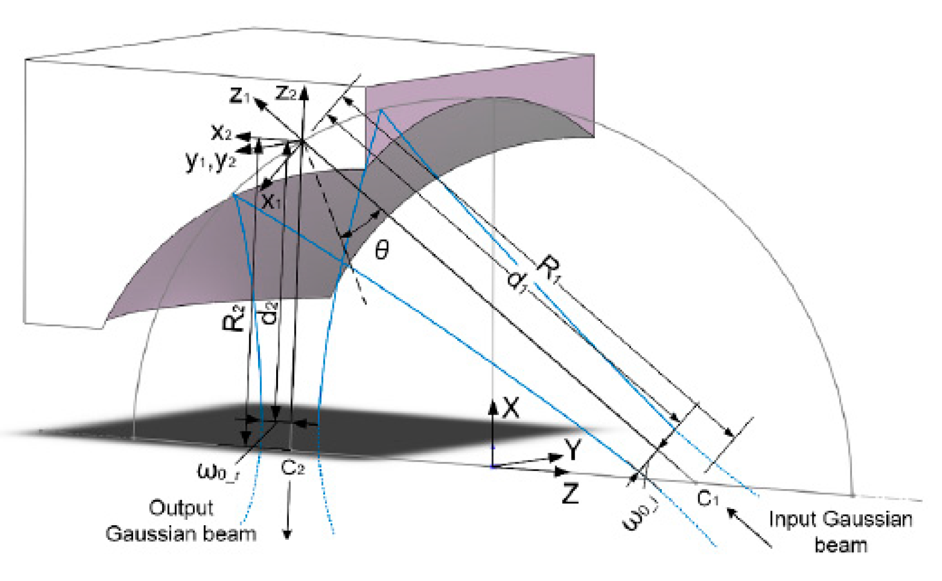
The analysis of a single off-axis reflector antenna and the transformation of co- and cross-polarization in a 2-D quasi-optical system were discussed in detail [19]. In brief, we choose an individual Hermite–Gaussian mode, for example, a $\left(p, q\right)$ Gaussian beam mode as the incident field to an offset mirror, the cross-polarization will emerge, and the co-polarization will be distorted as a result of the generated other order modes. The significant expressions of the input and output fields are given below, and the geometry of an off-axis ellipsoidal mirror with the incident and reflected beams in the local coordinate systems is plotted in Figure 1.

$$E_{\mathrm{i}-\mathrm{co}}=E_{pq}\exp \left[-\mathrm{j}{k}_0\left(z_1+d_1\right)-\frac{\mathrm{j}\pi \left({x_1}^2+{y_1}^2\right)}{\lambda R_{\mathrm{i}}}+\mathrm{j}\left(p+q+1\right){\varphi }_{\mathrm{i}}\right]$$

(1)

$$\begin{gathered} E_{\mathrm{r}-\mathrm{co}}\approx \mathrm{const}·{\displaystyle \sum }_{mn}\{u{1}_{mn-pq}{E}_{mn}\exp \left[\mathrm{j}{k}_0\left(z_2+d_2\right)+\frac{\mathrm{j}\pi \left({x_2}^2+{y_2}^2\right)}{\lambda R_{\mathrm{r}}}-\mathrm{j}\left(m+n+1\right){\varphi }_{\mathrm{r}}\right] \\ ·\exp \left(\mathrm{j}{\phi }_{mn-pq}\right)\exp \left(\mathrm{j}\pi \right)\} \end{gathered}$$

(2)

$$\begin{gathered} E_{\mathrm{r}-\mathrm{cx}}\approx \mathrm{const}·{\displaystyle \sum }_{m\left(n+1\right)}\{u{2}_{m\left(n+1\right)-pq}{E}_{m\left(n+1\right)}\exp \left[\mathrm{j}{k}_0\left(z_2+d_2\right)+\frac{\mathrm{j}\pi \left({x_2}^2+{y_2}^2\right)}{\lambda R_{\mathrm{r}}} \\ -\mathrm{j}\left(m+n+2\right){\varphi }_{\mathrm{r}}\right]·\exp \left(\mathrm{j}{\phi }_{m\left(n+1\right)-pq}\right)\exp \left(\mathrm{j}\pi \right)\} \end{gathered}$$

(3)

Here, $E_{\mathrm{i}-\mathrm{co}}$ is the co-polarization of the incident field linearly polarized in the $y$ direction, and $E_{\mathrm{r}-\mathrm{co}}$ and $E_{\mathrm{r}-\mathrm{cx}}$ are the co- and cross-polarization of the reflected field, respectively. $E_{pq}$ represents the amplitude of $\left(p, q\right)$ order Hermite–Gaussian mode. The exponential term in Equation (1) is the phase of $\left(p, q\right)$ order Hermite–Gaussian mode. In Equations (2) and (3), $u1$ and $u2$ are coefficients of co-polar modes and cx-polar modes, respectively. The last two exponential terms, $\exp \left(\mathrm{j}\phi \right)$ and $\exp \left(\mathrm{j}\pi \right)$, are additional phases to ensure the phase matching and phase reversal of the incident and reflected beams on the mirror according to the reflection theorem. Furthermore, the subscript $mn-pq$ means that the reflected $\left(m, n\right)$ mode is generated by the incident $\left(p, q\right)$ mode. The expressions of $u1$, $u2$, and $\phi$ were given in [19]. $k_0$ is the wavenumber. $d_{1/2}$ is the distance between the beam waist ${\omega }_{0\_\mathrm{i}/0\_\mathrm{r}}$ and the center of the mirror. $R_{\mathrm{i}/\mathrm{r}}$ and ${\varphi }_{\mathrm{i}/\mathrm{r}}$ are the radius of curvature and the phase slippage, respectively, which are functions of $z_{1/2}$. Furthermore, the relationship between parameters of the input and output Gaussian beams can be figured out by the ABCD matrix techniques [25,26]. From Equations (2) and (3), we can see that the reflected co-polarization will no longer be a single $\left(p, q\right)$ mode, which consists of a set of $\left(m, n\right)$ modes close to the $\left(p, q\right)$ mode. Additionally, the cross-polarization is composed of a set of $\left(m, n+1\right)$ modes.

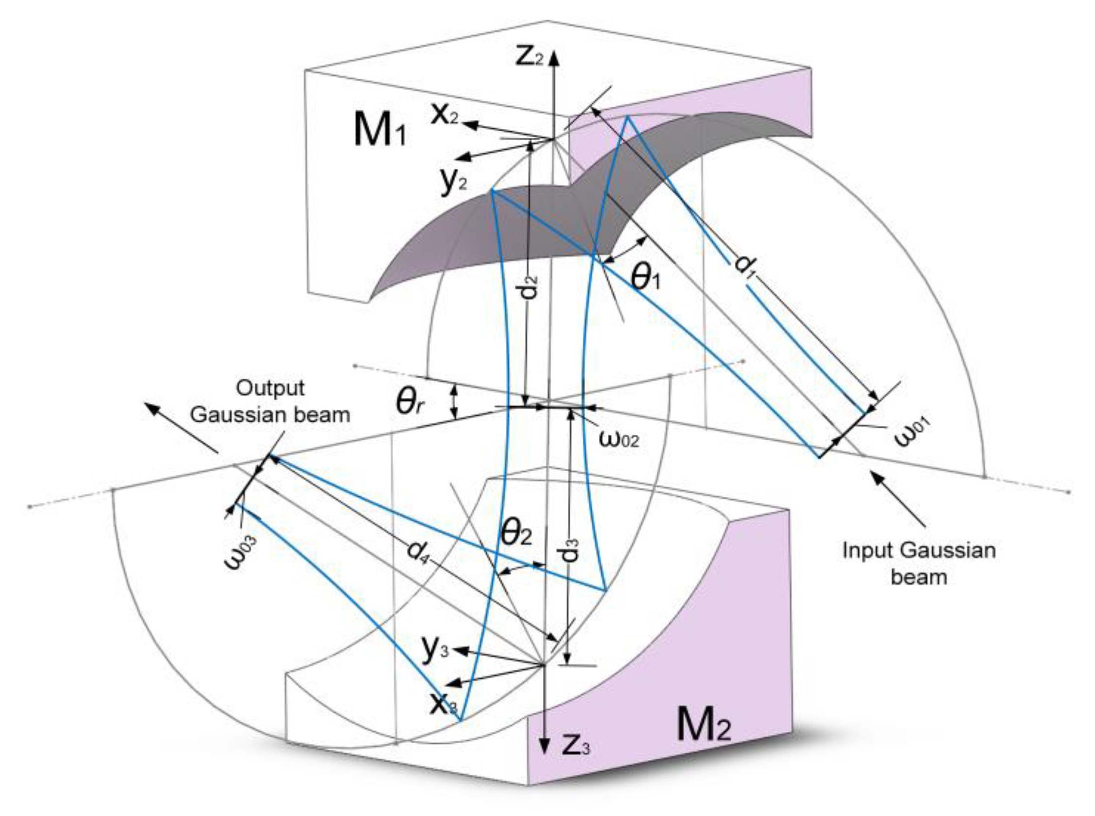
Different from 2-D quasi-optical systems in [19], the optical axes of beams are not on the same plane in 3-D systems. Referring to the analysis of a single offset reflector, we set up two coordinate systems of the output beam from the first mirror ${\mathrm{M}}_1$ and the input beam to the second mirror ${\mathrm{M}}_2$, as shown in Figure 2. It can be seen from the figure that there is a rotation angle ${\theta }_{\mathrm{r}}$ between two planes of optical axes of ${\mathrm{M}}_1$ and ${\mathrm{M}}_2$. Obviously, it becomes a 2-D system when ${\theta }_{\mathrm{r}}$ equals $0$ or $\pi$. In 3-D systems, some appropriate mode conversions and polarization conversions are essential to ensure that the reflected beams from ${\mathrm{M}}_1$ can be used as the incident beams to ${\mathrm{M}}_2$. Then, GBMA could be applied to analyze 3-D multi-reflector systems.

Figure 3 presents the view of $x_2{y}_2{z}_2$ and $x_3{y}_3{z}_3$ coordinate systems (shown in Figure 2) from the $z_3$-axis direction. From Figure 2 and Figure 3, two coordinates are connected by:

$$\{\begin{array}{c}{x}_2=\cos {\theta }_{\mathrm{r}}·x_3+\sin {\theta }_{\mathrm{r}}·y_3\\ y_2=\sin {\theta }_{\mathrm{r}}·x_3-\cos {\theta }_{\mathrm{r}}·y_3\\ z_2=-z_3-\left(d_2+d_3\right) \end{array}$$

(4)

where $d_2$ and $d_3$ are the distances from the beam waist ${\omega }_{02}$ to ${\mathrm{M}}_1$ and to ${\mathrm{M}}_2$, respectively. Therefore, $d_2+d_3$ is the distance between the two mirrors. Apparently, the modes of reflected waves from ${\mathrm{M}}_1$ are in the $x_2{y}_2{z}_2$ coordinate system. These modes must be converted into a new set of modes in the $x_3{y}_3{z}_3$ system to fit ${\mathrm{M}}_2$. Now, substitute Equation (4) into Equation (2):

$$\begin{gathered} E_{\mathrm{r}-\mathrm{co}}\approx \mathrm{const}·{{\displaystyle \sum }}_{mn}\{u{1}_{mn-pq}{E}_{mn}\left(x_2,y_2,z_2\right)\exp \left[-\mathrm{j}{k}_0\left(z_3+d_3\right)-\frac{\mathrm{j}\pi \left({x_3}^2+{y_3}^2\right)}{\lambda R_{\mathrm{i}}\left(z_3\right)}+ \\ \mathrm{j}\left(m+n+1\right){\varphi }_{\mathrm{i}}\left(z_3\right)\right]·\exp \left(\mathrm{j}{\phi }_{mn-pq}\right)\exp \left(\mathrm{j}\pi \right)\}. \end{gathered}$$

(5)

In the process of replacing $x_2,y_2,z_2$ with $x_3,y_3,z_3$, the functions $R_{\mathrm{r}}\left(z_2\right)$ and ${\varphi }_{\mathrm{r}}\left(z_2\right)$ in Equation (2) can be written as $-R_{\mathrm{i}}\left(z_3\right)$ and $-{\varphi }_{\mathrm{i}}\left(z_3\right)$, and then we can obtain Equation (5). The expression of cross-polarization is similar to this and not given here. The amplitude $E_{mn}\left(x_2,y_2,z_2\right)$ of the $\left(m, n\right)$ Gaussian beam mode needs to be further discussed, which is a function of $x_2$, $y_2$, and $z_2$.

$$\begin{array}{l}{E}_{mn}\left(x_2,y_2,z_2\right)\\ ={\left[2^{m+n+1}m!n!\pi \omega {\left(z_2\right)}^2\right]}^{-0.5}{H}_m\left[\frac{\sqrt{2}{x}_2}{\omega \left(z_2\right)}\right]H_n\left[\frac{\sqrt{2}{y}_2}{\omega \left(z_2\right)}\right]\exp \left[-\frac{{x_2}^2+{y_2}^2}{\omega {\left(z_2\right)}^2}\right]\end{array}$$

(6)

where $\omega \left(z_2\right)$ represents the beam radius and $H_m\left(u\right)$ is the $m$ order Hermite polynomial.

$$\omega \left(z_2\right)={\omega }_{02}{\left\{1+{\left[\frac{\lambda \left(-z_2-d_2\right)}{\pi {{\omega }_{02}}^2}\right]}^2\right\}}^{0.5}$$

(7)

where ${\omega }_{02}$ is the beam waist radius of the output wave from ${\mathrm{M}}_1$, which is also the beam waist radius of the input wave to ${\mathrm{M}}_2$. Then, we obtain $\omega$ in the $x_3{y}_3{z}_3$ coordinate system.

$$\omega \left(z_3\right)={\omega }_{02}{\left\{1+{\left[\frac{\lambda \left(z_3+d_3\right)}{\pi {{\omega }_{02}}^2}\right]}^2\right\}}^{0.5}$$

(8)

Combining Equation (4), Equation (6), Equation (7), and Equation (8), we could obtain the formula of $E_{mn}$($x_3,y_3,z_3$).

$$\begin{gathered} E_{mn}\left(x_3,y_3,z_3\right)={\left[2^{m+n+1}m!n!\pi \omega {\left(z_3\right)}^2\right]}^{-0.5}{H}_m\left[\frac{\sqrt{2}\left(\cos {\theta }_{\mathrm{r}}·x_3+\sin {\theta }_{\mathrm{r}}·y_3\right)}{\omega \left(z_3\right)}\right]H_n\left[\frac{\sqrt{2}\left(\sin {\theta }_{\mathrm{r}}·x_3-\cos {\theta }_{\mathrm{r}}·y_3\right)}{\omega \left(z_3\right)}\right] \\ ·\exp \left[-\frac{{x_3}^2+{y_3}^2}{\omega {\left(z_3\right)}^2}\right] \end{gathered}$$

(9)

Then, according to the expressions of Hermite polynomials, we could transform the amplitude $E_{mn}$ of a single $\left(m, n\right)$ mode into the amplitude sum of a new set of modes in the $x_3{y}_3{z}_3$ system. Here, we give three simple results of the mode conversion. By the way, these three modes are generated by one reflection of the fundamental mode [11].

$$\begin{gathered} E_{00}\left(x_2,y_2,z_2\right)=E_{00}\left(x_3,y_3,z_3\right) \\ {E}_{12}\left(x_2,y_2,z_2\right)=-\sqrt{3}{\cos }^2{\theta }_{\mathrm{r}}\sin {\theta }_{\mathrm{r}}·E_{03}\left(x_3,y_3,z_3\right)+\sqrt{3}\cos {\theta }_{\mathrm{r}}{\sin }^2{\theta }_{\mathrm{r}}·E_{30}\left(x_3,y_3,z_3\right) \\ +\left({\cos }^3{\theta }_{\mathrm{r}}-2\cos {\theta }_{\mathrm{r}}{\sin }^2{\theta }_{\mathrm{r}}\right)E_{12}\left(x_3,y_3,z_3\right)+\left(-{\sin }^3{\theta }_{\mathrm{r}}-2{\cos }^2{\theta }_{\mathrm{r}}\sin {\theta }_{\mathrm{r}}\right)E_{21}\left(x_3,y_3,z_3\right) \\ {E}_{30}\left(x_2,y_2,z_2\right)=-{\sin }^3{\theta }_{\mathrm{r}}·E_{03}\left(x_3,y_3,z_3\right)+{\cos }^3{\theta }_{\mathrm{r}}·E_{30}\left(x_3,y_3,z_3\right) \\ +\left(\sqrt{3}/2\right)\cos {\theta }_{\mathrm{r}}{\sin }^2{\theta }_{\mathrm{r}}·E_{12}\left(x_3,y_3,z_3\right)-\left(\sqrt{3}/2\right){\cos }^2{\theta }_{\mathrm{r}}\sin {\theta }_{\mathrm{r}}·E_{21}\left(x_3,y_3,z_3\right) \\ +\left(\sqrt{6}/4\right)\left(-{\sin }^3{\theta }_{\mathrm{r}}+\sin {\theta }_{\mathrm{r}}\right)E_{01}\left(x_3,y_3,z_3\right)+\left(\sqrt{6}/4\right)\left({\cos }^3{\theta }_{\mathrm{r}}-\cos {\theta }_{\mathrm{r}}\right)E_{10}\left(x_3,y_3,z_3\right) \end{gathered}$$

(10)

By substituting Equation (10) into Equation (5), the formula for the co-polarization in the x₃y₃z₃ coordinate system will be obtained. We need to pay attention to the fact that the phase $\left(m+n+1\right){\varphi }_{\mathrm{i}}$ in Equation (5) is the phase of the $\left(m, n\right)$ mode. However, there is not only the $\left(m, n\right)$ mode but also other modes after the mode conversion. Therefore, to achieve modular computing, we apply the same way in Equation (10) in [11] to approximate the phase $\left(m+n+1\right){\varphi }_{\mathrm{i}}$ so that it can be paired with modes other than the (m, n) mode. Only when the sum of x and $y$ directional orders of the new modes is not equal to that of the original mode, that is, $m_{\mathrm{new}}+n_{\mathrm{new}}\ne m+n$, the phase $\left(m+n+1\right){\varphi }_{\mathrm{i}}$ needs to be replaced by the phase $\left(m_{\mathrm{new}}+n_{\mathrm{new}}+1\right){\varphi }_{\mathrm{i}}$.

Since the converted modes and the original modes are essentially the same fields, the condition of phase matching between the new mode $\left(m_{\mathrm{new}}, n_{\mathrm{new}}\right)$ and the mode $\left(p, q\right)$ still needs to be met on ${\mathrm{M}}_1$. Therefore, the additional phase term in Equation (5), ${\phi }_{mn-pq}$, needs to be replaced by ${\phi }_{m_{\mathrm{new}}{n}_{\mathrm{new}}-pq}$, when $m_{\mathrm{new}}+n_{\mathrm{new}}$ is not equal to $m+n$. Finally, a new set of modes and coefficients in the $x_3{y}_3{z}_3$ coordinate system will be obtained. After the mode conversion, the co-polarization can be written in the form of a set of $\left(m_{\mathrm{new}}, n_{\mathrm{new}}\right)$ modes:

$$\begin{gathered} E_{\mathrm{r}-\mathrm{co}}\approx \mathrm{const}·{\displaystyle \sum }_{m_{\mathrm{new}}{n}_{\mathrm{new}}}\{u{1^{\prime }}_{m_{\mathrm{new}}{n}_{\mathrm{new}}-pq}{E}_{m_{\mathrm{new}}{n}_{\mathrm{new}}}\exp \left[-\mathrm{j}{k}_0\left(z_3+d_3\right)-\frac{\mathrm{j}\pi \left({x_3}^2+{y_3}^2\right)}{\lambda R_{\mathrm{i}}}+\mathrm{j}\left(m_{\mathrm{new}}+n_{\mathrm{new}}+1\right){\varphi }_{\mathrm{i}}\right] \\ ·\exp \left(\mathrm{j}{\phi }_{m_{\mathrm{new}}{n}_{\mathrm{new}}-pq}\right)\exp \left(\mathrm{j}\pi \right)\}. \end{gathered}$$

(11)

Here, $u{1^{\prime }}_{m_{\mathrm{new}}{n}_{\mathrm{new}}-pq}$ is the coefficient of the $\left(m_{\mathrm{new}}, n_{\mathrm{new}}\right)$ mode, which is a function of the mode order and the rotation angle ${\theta }_{\mathrm{r}}$, and can be obtained from the above analysis. For example, the coefficients of new modes converted from $\left(0, 0\right)$, $\left(1, 0\right)$, and $\left(1, 0\right)$ modes can be obtained from Equation (10). $E_{m_{\mathrm{new}}{n}_{\mathrm{new}}}$ is the amplitude term of the $\left(m_{\mathrm{new}}, n_{\mathrm{new}}\right)$ mode. $\exp \left(\mathrm{j}{\phi }_{m_{\mathrm{new}}{n}_{\mathrm{new}}-pq}\right)$ and $\exp \left(\mathrm{j}\pi \right)$ are additional phase terms.

Up to now, the mode conversion was fully described. In the following part, we will give details about the polarization conversion. According to the previous analyses, the co-polarization $E_{\mathrm{r}-\mathrm{co}-{\mathrm{M}}_1}$ and the cross-polarization $E_{\mathrm{r}-\mathrm{cx}-{\mathrm{M}}_1}$ reflected from ${\mathrm{M}}_1$ are linearly polarized in the $y_2$ and $x_2$ directions, respectively. Similarly, we should convert these two orthogonal polarizations into linear polarizations in the $x_3{y}_3{z}_3$ system after the mode conversion. First, the original co- and cross-polarization need to be decomposed into two components in the $x_3$ and $y_3$ directions. $E_{\mathrm{r}-\mathrm{co}-{\mathrm{M}}_1}$ can be decomposed into $\cos {\theta }_{\mathrm{r}}·E_{\mathrm{r}-\mathrm{co}-{\mathrm{M}}_1}$ and $\sin {\theta }_{\mathrm{r}}·E_{\mathrm{r}-\mathrm{co}-{\mathrm{M}}_1}$, which are linearly polarized in the $y_3$ and $x_3$ directions, respectively. Furthermore, $E_{\mathrm{r}-\mathrm{cx}-{\mathrm{M}}_1}$ can be decomposed into $\sin {\theta }_{\mathrm{r}}·E_{\mathrm{r}-\mathrm{cx}-{\mathrm{M}}_1}$ and $\cos {\theta }_{\mathrm{r}}·E_{\mathrm{r}-\mathrm{cx}-{\mathrm{M}}_1}$, which are linearly polarized in the $y_3$ and $x_3$ directions, respectively. Second, the decomposed co- and cross-polarization in the same direction, for example, the $x_3$ or $y_3$ direction, need to be accumulated to obtain two new polarizations linearly polarized in the $x_3$ and $y_3$ directions. Whether these components are added or subtracted depends on the rotation angle ${\theta }_{\mathrm{r}}$. We have modelled and simulated various systems, including the systems with two, three or more reflectors, the feeds with or without cross-polarization, the feeds containing one, two or more Gaussian beam modes, and so on. Through the calculation and analysis of these systems, we finally obtained the following equation, which can correctly calculate the converted co- and cross-polarization.

$$\{\begin{array}{c}\{\begin{array}{c}{E}_{{i}-\mathrm{co}-{{M}}_2}=\cos {\theta }_{{r}}·E_{{r}-\mathrm{co}-{{M}}_1}-\sin {\theta }_{{r}}·E_{{r}-\mathrm{cx}-{{M}}_1} \\ E_{{i}-\mathrm{cx}-{{M}}_2}=-\sin {\theta }_{{r}}·E_{{r}-\mathrm{co}-{{M}}_1}+\cos {\theta }_{{r}}·E_{{r}-\mathrm{cx}-{{M}}_1}\end{array}\\ \mathrm{with}(0\le {\theta }_{{r}}<\frac{\pi }{4},\frac{3\pi }{4}\le {\theta }_{{r}}<\frac{5\pi }{4},\frac{7\pi }{4}\le {\theta }_{{r}}<2\pi )\\ \{\begin{array}{c}{E}_{{i}-\mathrm{co}-{{M}}_2}=\cos {\theta }_{{r}}·E_{{r}-\mathrm{co}-{{M}}_1}+\sin {\theta }_{{r}}·E_{{r}-\mathrm{cx}-{{M}}_1} \\ E_{{i}-\mathrm{cx}-{{M}}_2}=\sin {\theta }_{{r}}·E_{{r}-\mathrm{co}-{{M}}_1}+\cos {\theta }_{{r}}·E_{{r}-\mathrm{cx}-{{M}}_1} \end{array}\\ \mathrm{with}(\frac{\pi }{4}\le {\theta }_{{r}}<\frac{3\pi }{4},\frac{5\pi }{4}\le {\theta }_{{r}}<\frac{7\pi }{4})\end{array}$$

(12)

Here, the subscripts $\mathrm{i}-\mathrm{co}-{\mathrm{M}}_2$ and $\mathrm{r}-\mathrm{cx}-{\mathrm{M}}_1$ mean the co-polarization of the incident beam to ${\mathrm{M}}_2$ and the cross-polarization of the reflected beam from ${\mathrm{M}}_1$.

Ultimately, we will obtain the new co- and cross-polarization in the $x_3{y}_3{z}_3$ coordinate system by substituting $E_{\mathrm{r}-\mathrm{co}-{\mathrm{M}}_1}$ and $E_{\mathrm{r}-\mathrm{cx}-{\mathrm{M}}_1}$ into Equation (12). $E_{\mathrm{r}-\mathrm{co}-{\mathrm{M}}_1}$ can be calculated by Equation (11) and $E_{\mathrm{r}-\mathrm{cx}-{\mathrm{M}}_1}$ can be obtained in a similar way. It should be noted that $E_{\mathrm{r}-\mathrm{co}-{\mathrm{M}}_1}$ and $E_{\mathrm{r}-\mathrm{cx}-{\mathrm{M}}_1}$ are the fields after the mode conversion. Then, $E_{\mathrm{i}-\mathrm{co}-{\mathrm{M}}_2}$ and $E_{\mathrm{i}-\mathrm{cx}-{\mathrm{M}}_2}$ can be used as the incident fields to the next mirror ${\mathrm{M}}_2$.

Finally, 3-D multi-reflector quasi-optical systems can be analyzed by 3-D GBMA. With 3-D GBMA, the proportion of different Gaussian beam modes in the system can be calculated accurately, which can be used to analyze the performance of the system. At the same time, the amplitude and phase field distribution at any position in the system can be evaluated quickly, which directly shows the electrical properties. Therefore, 3-D GBMA can be considered to be very useful for system analysis and design.

3. Results and Discussion

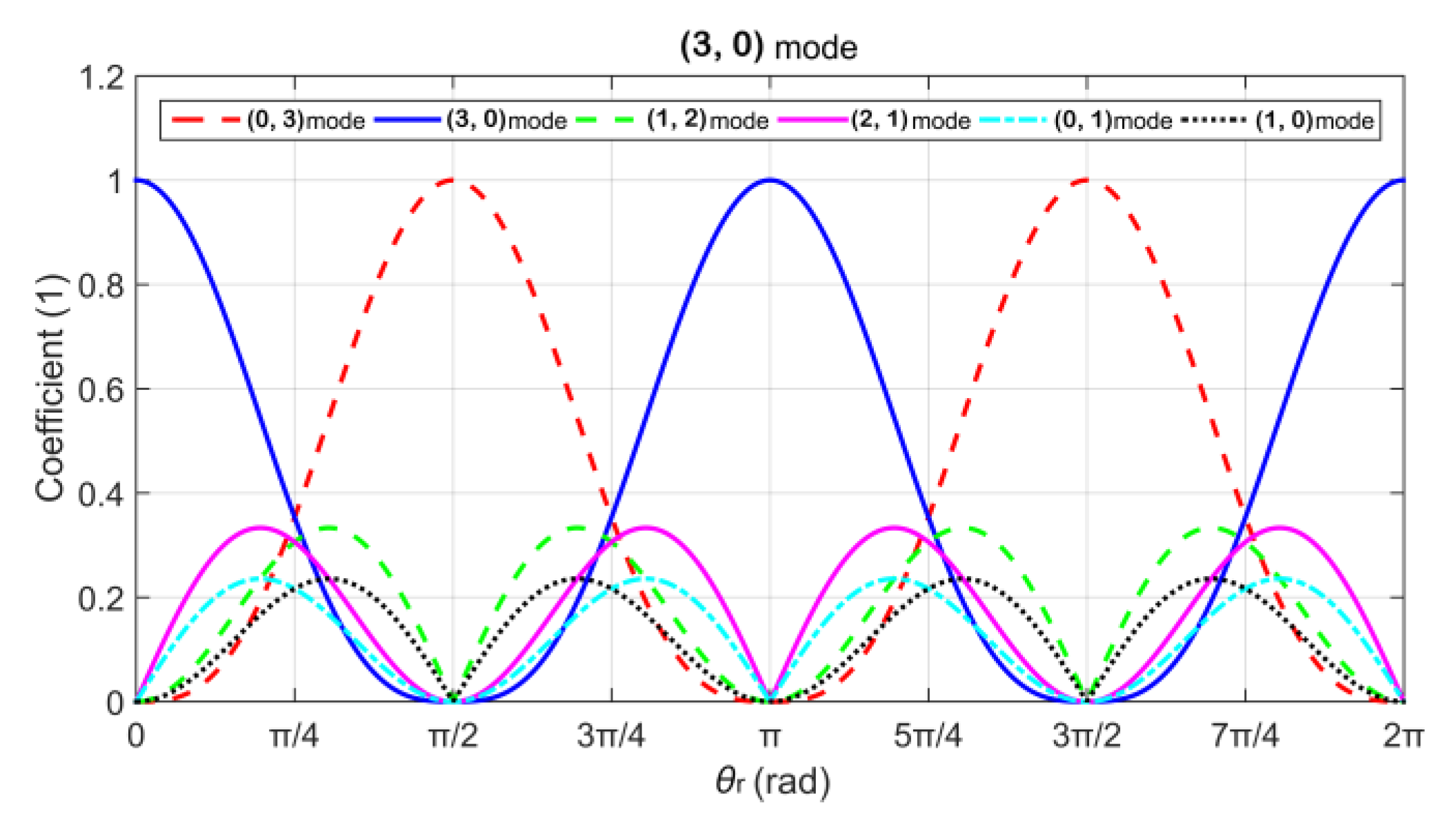
First, the rationality of the approximate calculation of the phase mentioned above will be analyzed. There are three modes, $\left(0, 0\right)$, $\left(1, 2\right)$, and $\left(3, 0\right)$, reflected from ${\mathrm{M}}_1$ with the fundamental Gaussian beam mode incident to ${\mathrm{M}}_1$. These three modes need to be converted to match the next mirror ${\mathrm{M}}_2$. According to the previous analysis of the mode conversion and Equation (10), only the mode $\left(3, 0\right)$ will be converted to other modes that meet the condition $m_{\mathrm{new}}+n_{\mathrm{new}}\ne m+n$. In Figure 4, we show the curves of the coefficients of the new modes, varying with ${\theta }_{\mathrm{r}}$ in the example of $\left(3, 0\right)$ mode. The coefficients of new modes can be calculated by Equation (10). We can find that coefficients of other modes remain low through the process of ${\theta }_{\mathrm{r}}$ varying, except $\left(3, 0\right)$ and $\left(0, 3\right)$ modes, which means that the energy of other modes is kept at a low level, and its influence on $\left(3, 0\right)$ and $\left(0, 3\right)$ modes is small. In addition, coefficients of $\left(0, 1\right)$ and $\left(1, 0\right)$ modes that need to be approximated for phase remain at a low level, so the impact of the approximation is relatively low. In addition, the energy of $\left(0, 1\right)$ and $\left(1, 0\right)$ modes reaches a high level with ${\theta }_{\mathrm{r}}$ approaching $\pi /4$, $3\pi /4$, etc., which means that the effect of approximation is great in these cases.

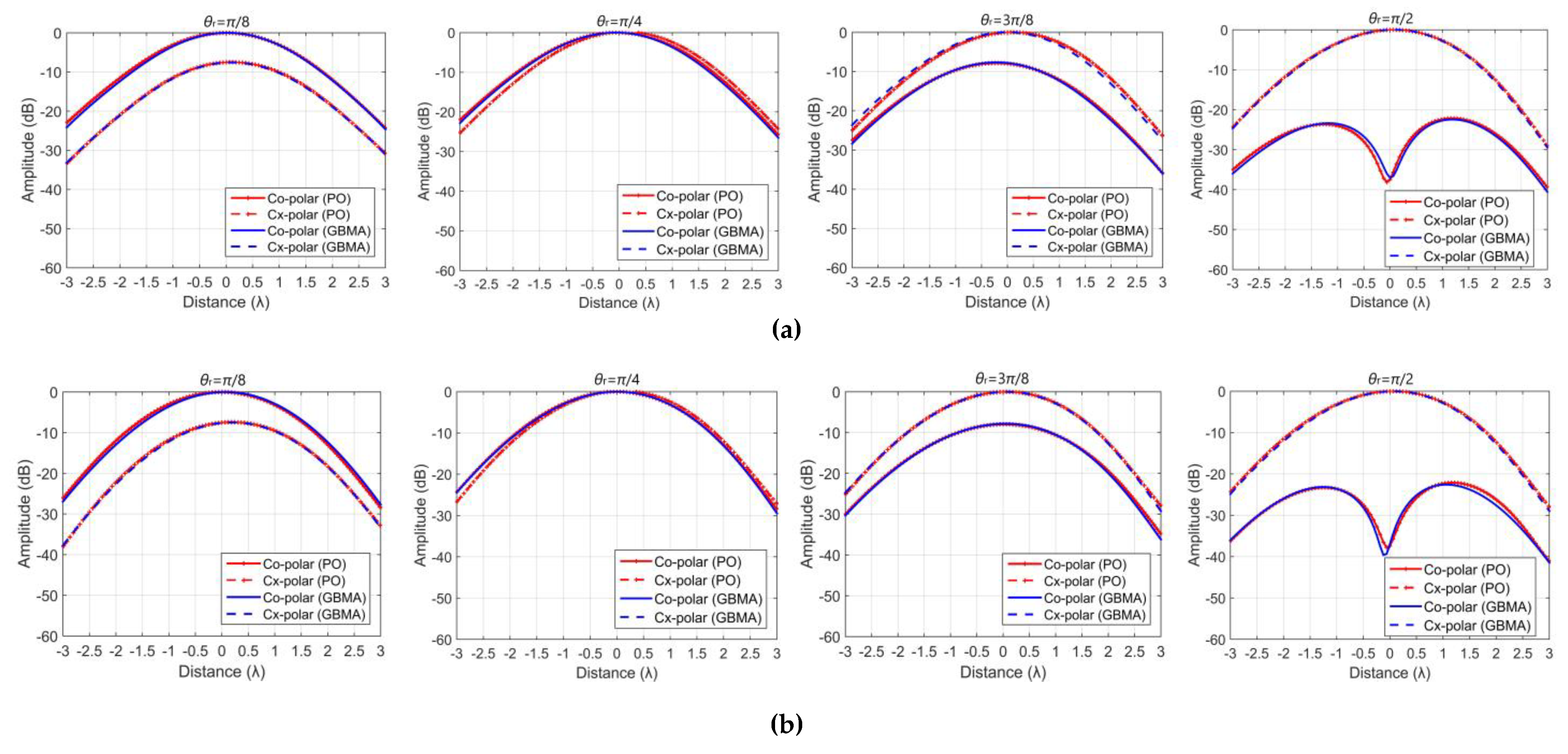
The further accuracy analysis of 3-D GBMA will be given below, verified by the simulated and measured results of 3-D double ellipsoidal reflector systems. To make the whole process easier to understand, we select a fundamental mode Gaussian beam feed without cross-polarization and two identical mirrors to compose the systems with different ${\theta }_{\mathrm{r}}$. The details of the feed and reflector are given in

Table 1. Parameters of Feed and Reflector.

Feed	Values	Reflector	Values
Frequency	183 GHz	Distance R1	47λ
Wavelength	λ	Distance R2	86.29λ
Beam waist radius ω01	1.67λ	Incident angle θ	π/6
		Diameter D	35.20λ

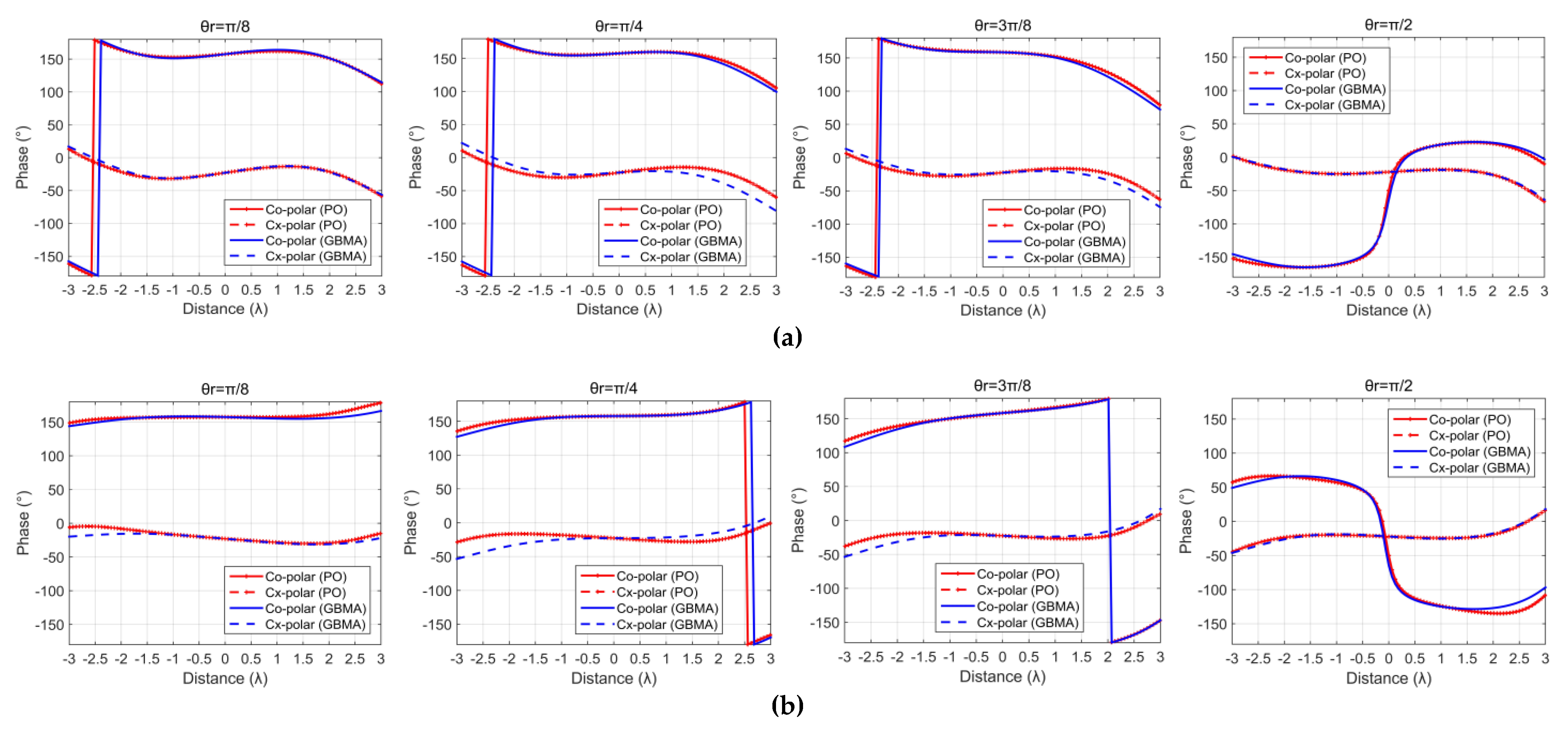
. It is worth mentioning that the proposed 3-D GBMA is programmed in MATLAB. The commercial electromagnetic simulation software GRASP based on PO is used as a contrast. We can model and calculate different systems with the parameters of the feed and reflector in Table 1 and different rotation angles ${\theta }_{\mathrm{r}}$. Then, we present near-field amplitude and phase distributions on the plane of the beam waist ${\omega }_{03}$ (shown in Figure 2) in 3-D systems with different ${\theta }_{\mathrm{r}}$ in Figure 5 and Figure 6.

These amplitude results of 3-D GBMA are in good agreement with those of PO within the range of twice the beam radius. The polarization direction of the feed is chosen to define the co- and cross-polarization direction of the system. The mutual conversion between the co- and cross-polarization is caused by the change of ${\theta }_{\mathrm{r}}$. It is not hard to see that cross-polarization is higher than co-polarization with ${\theta }_{\mathrm{r}}=\pi /2$. The maximum difference between the two results is less than 2.6 dB, which occurs on the edge of the sampling plane with the rotation angle ${\theta }_{\mathrm{r}}$ equal to $\pi /4$. Here, the results of two special 3-D systems with ${\theta }_{\mathrm{r}}=0$ and $\pi$ are no longer given, which have been presented in [19]. As ${\theta }_{\mathrm{r}}$ increases from 0 to $\pi /4$, the difference is increasing. Then, the difference drops until ${\theta }_{\mathrm{r}}$ equals $\pi /2$. From the phase results, we can obtain the same conclusions. The maximum difference is less than 24.7° on the edge of the sampling plane with ${\theta }_{\mathrm{r}}=\pi /4$. The reason is that the approximate calculation of phase is used in the mode conversion.

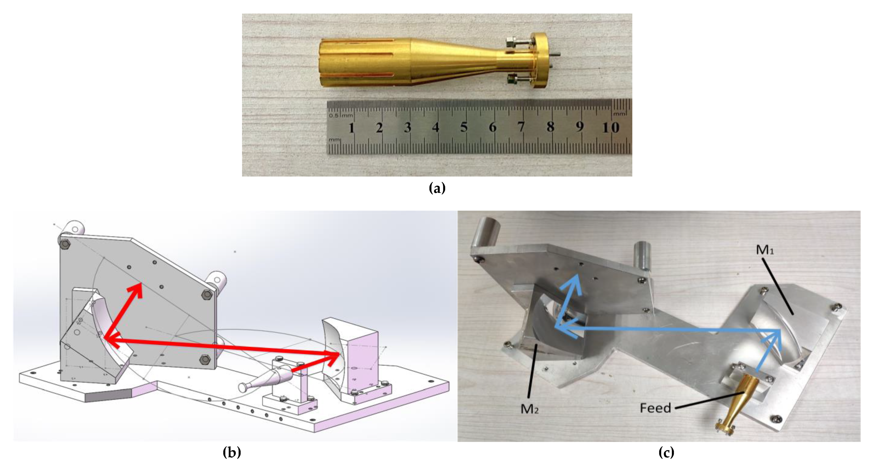
Following, we present detailed information about the fabrication and measurement of a system with ${\theta }_{\mathrm{r}}=\pi /2$ to verify the accuracy of 3-D GBMA further. The prototypes of the corrugated horn and the fabricated double ellipsoidal reflector systems are illustrated in Figure 7. The parameters of the corrugated horn and manufactured reflectors are also consistent with those given in Table 1. The Root Mean Square (RMS) surface tolerance of mirrors is less than 5 microns.

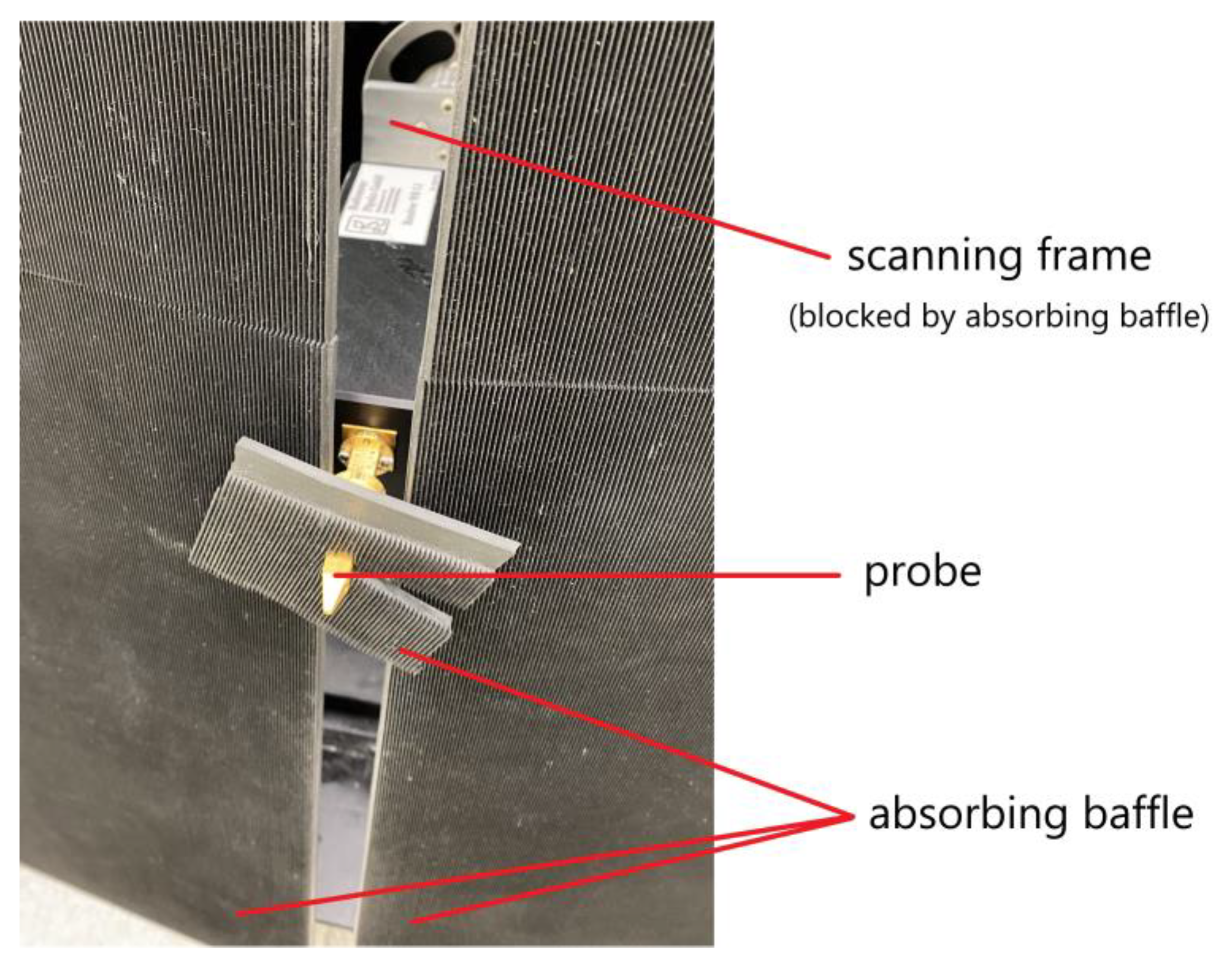
We applied near field scanning to measure the output electric field from this system. Figure 8 presents the scanning devices, including the probe, scanning frame and absorbing baffle. The scanning plane is chosen at a distance of 200 mm from the beam waist ${\omega }_{03}$ (shown in Figure 2). The dimension of the measured plane is 212 mm by 212 mm, which covers a range of two times the beam radius. 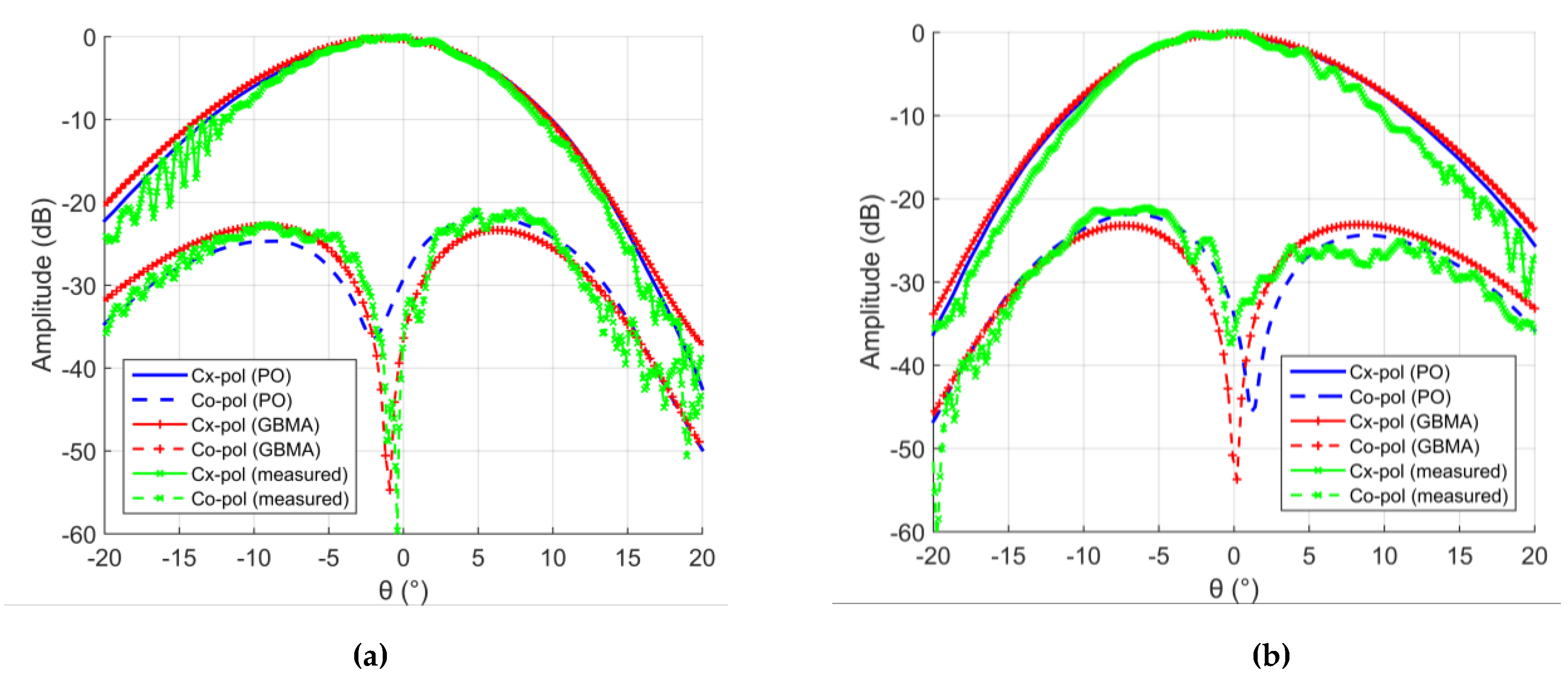The number of sampling points is 143*143, and the sampling interval is 1.49 mm, slightly less than $\mathsf{\lambda }$ at 183 GHz. Furthermore, the far field results are calculated by performing Fast Fourier Transform (FFT) on the near field data. 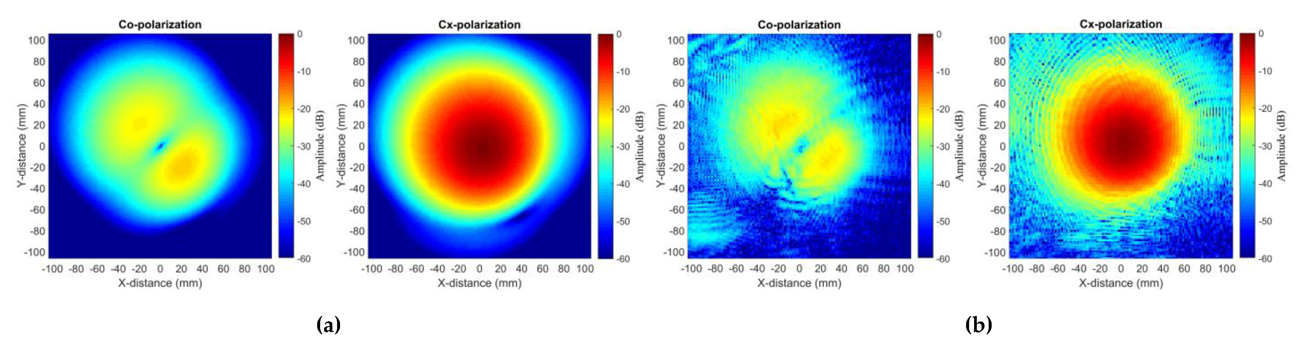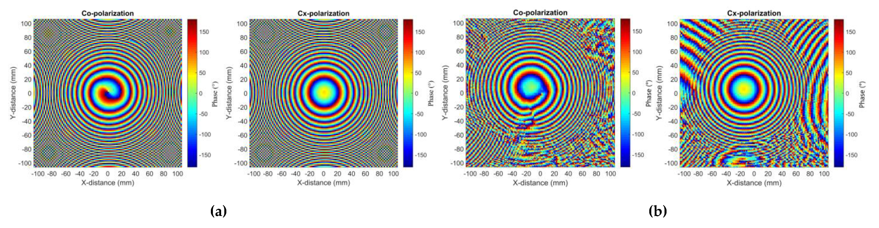The far field radiation patterns on E- and H-planes are plotted in Figure 9, including the simulated results of 3-D GBMA and PO and the measured results. The near field results on the scanning plane are given in Figure 10 and Figure 11. It should be noted that the radiation field from the corrugated horn contains not only the fundamental Gaussian beam, but also some higher order modes with very low energy. The purity of the fundamental Gaussian beam mode in the horn feed is about 99.8%, and there is a cross-polarization with a peak amplitude of about −30 dB. In the simulations, two single fundamental Gaussian beam modes with peaks of 0 dB and −30 dB are used to approximate the co- and cross-polarization in the horn, respectively, which caused a small difference between the simulated and measured results. Furthermore, the ripples of measured results are caused by the background noise, the reflection, and diffraction of various metal surfaces. However, we can still see that the differences between these three results are acceptable. Moreover, we can find that the amplitudes and phases simulated by 3-D GBMA and measured are very similar through observing the near field results. Finally, we can conclude that both the amplitude and phase of the co- and cross-polarization are simulated by 3-D GBMA accurately, and 3-D GBMA is correct and precise compared with PO and the measured results. Now, the calculation efficiency of 3-D GBMA will be discussed and compared with PO in GRASP10. We program 3-D GBMA in MATLAB. It should be noted that the calculation speed is not optimized, such as parallel computing. The execution time of 3-D GBMA and PO in the 3-D dual-reflector system with ${\theta }_{\mathrm{r}}=\pi /2$ is given in

Table 2. Execution time of 3-D GBMA and PO.

Method	First Reflection	Mode Conversion	Polarization Conversion	Second Reflection	Field	Total
3-D GBMA	0.08 s	0.13 s	0.06 s	0.17 s	0.08 s	0.52 s
PO (single-core)	0.52 s	-	-	15.92 s	3.71 s	20.15 s
PO (multi-core)	0.42 s	-	-	3.85 s	0.54 s	4.81 s

Note: The computer configuration is as follows: 6 cores and 12 threads Central Processing Unit (CPU), 16 GB Random Access Memory (RAM), 256 GB Solid State Disk (SSD).

. In the first reflection, 3-D GBMA takes 0.08s to compute the modes, and PO (single-core) takes 0.52 s to obtain the currents on ${\mathrm{M}}_1$. Then, the consuming time of the mode and polarization conversions is 0.13 s and 0.06 s, respectively. In the second reflection, 3-D GBMA and PO (single-core) take 0.17 s and 15.92 s. Finally, two methods cost 0.08 s and 3.71 s to calculate the field distributions. It is worth noting that the time of 3-D GBMA in Table 2 is executed in the single-core, which can be further reduced with the multi-core parallel computing. In addition, the execution time of PO in the multi-core operation is also given as a reference. We can conclude that 3-D GBMA is efficient and accurate compared with PO in GRASP10.

4. Conclusions

In this work, GBMA is further improved to be applied to analyze 3-D quasi-optical systems. Some significant expressions and derivation processes are given and discussed in detail. To verify the validity and accuracy of 3-D GBMA, we compared the results with those obtained by PO in GRASP10 of several 3-D dual-reflector systems with different rotation angles. To realize modular computation and improve efficiency, we made some approximations at the expense of some accuracy. The maximum difference between the two methods’ results is less than 2.6 dB in amplitude and 24.7° in phase at the edge of twice the beam radius on the sampling plane. Moreover, we fabricated a 3-D double ellipsoidal reflector system with θ_r = π/2, and applied near field scanning. The measured results are in good agreement with the simulated results for both co- and cross-polarization. Furthermore, the calculation efficiency of 3-D GBMA was compared with PO in GRASP10. Taking a 3-D dual-reflector system as an example, the execution time of 3-D GBMA is much shorter than that of PO with the same computing resources. Finally, we could conclude that 3-D GBMA is correct, accurate and efficient to calculate the field distribution in multi-reflector quasi-optical systems.