Bridge Dynamic Cable-Tension Estimation with Interferometric Radar and APES-Based Time-Frequency Analysis

Abstract

Dynamic cable-tension is an important bridge-health indicator. However, it is difficult to be measured precisely and efficiently. A remote bridge dynamic cable-tension measurement method is proposed. It uses an interferometric radar sensor, a time-frequency analysis technique, and a tension estimation approach based on a string-vibration-equation. One radar can measure the displacements of multiple cables aligned on one side of a bridge, at the same time. By solving the string vibration equation, each cable-tension is calculated from its fundamental frequency, which is obtained by time-frequency analyzing a short section of the cable’s whole displacement vector in an overlapped-piecewise manner. An adaptive amplitude and phase estimation (APES) algorithm is used to solve the frequency resolution deterioration problem due to the short duration. Simulations and field experiments with a K band interferometric radar validate that the proposed method is superior to traditional cable-tension measurements in terms of precision, robustness, and efficiency. The proposed method is of great application value in measuring and monitoring large cable-stayed bridges and cable-suspended bridges.

1. Introduction

Cable-stayed bridges and suspension bridges are the first choices to build long-span bridges to cross rivers and seas [1]. Cables are vital structural anchors and force-bearing components of a bridge. A long-span bridge is composed of serval groups of cables. Each cable-tension should be designed appropriately to achieve rational deck alignment and internal-force distribution. Many bridge disasters result from cable failures. Therefore, the cable-tension must be measured accurately during the whole bridge-life-cycle, including the construction stage, the traffic-operating period, and the renovation phase [2].

There are various methods to measure cable-tension, such as the pressure gauge measurement, the magneto-elastic based method [3], and the vibration-frequency based method [4]. The vibration-frequency based cable-tension measurement is the most widely used method due to its simple applicability and good adaptability. Vibration frequency measuring sensors can be roughly classified into cable-contact measuring ones and remote measuring ones. Sensors of the first kind include accelerometers and vibration pickups. [5]. These sensors usually have to be bound near the lower ends of the cables for convenience, when no lift truck is available to raise the sensors to higher positions. Because the lower ends are usually connected to various types of vibration absorbers or anchorage devices, the sensors mounted at lower positions would fail to get satisfactory measuring results. Sensors of the second kind include vision-based sensors and interferometric radars [6,7,8,9]. Vision-based sensors generally require a reflector installed on a cable to improve the measuring precision. Besides, their performances tend to decrease in adverse weather. On the other hand, interferometric radars are immune to adverse weather and require no additional reflectors. Since they are precise and efficient to measure multiple cables by only one snapshot, interferometric radars are accepted by more bridge engineers. A rapid and dynamic cable-tension measurement has drawn more attraction in a bridge health monitor application. The interferometric radar will be a potential sensor to meet these special requirements.

Cable displacements are first measured by an interferometric radar and then transformed into the spectrum domain [8]. The cable-tension can be obtained by solving the stay-cable free vibration differential equation [5] at last. The first step has been verified by numerous experiments [10]. The last step is also well studied by taking factors, such as damper, bending stiffness, and temperature variation, into considerations [4,11]. However, it is often taken for granted that the middle step works well with the conventional fast Fourier transform (FFT). The widely used FFT method would be affected by high sidelobes, which makes it hard to distinguish the peak of a weak target from the sidelobes of a strong one. Although the sidelobes can be suppressed by weighting the input displacement, it would cause a main lobe expansion problem at the same time. ZOOM-FFT (ZFFT), FFT-Fourier Series (FFT-FS), and chirp z-transform (CZT) are proposed to improve the computation resolution. These FFT-based methods still suffer limited frequency resolution that is in inverse proportion to the time duration [12]. Besides, they cannot give an accurate frequency peak due to sidelobe leakage from a nearby component. Park et al. have proposed a noniterative frequency estimation method for a single sinusoidal model [13]. By properly setting the phase interval, it can achieve good performance when Gaussian noise and harmonic components are present. Giarnetti et al. have proposed a parametric method to non-recursively estimate the frequency of multi-harmonic sinusoidal, especially with short duration [14]. The method is computationally efficient and it is very suitable for time-frequency distribution analysis, as a reference frequency required can be determined by the last result. However, both models do not match the actual model of bridge-cable deformation, as there are other unknown sinusoidal interferences. By using fast Hartley’s transform, the computation efficiency can further be improved since the input vector is real data [15].

Adaptive spectral estimation can give more precise results if the time-domain data can be modeled as a sum of multiple sinusoidal signals. Cable displacement waveforms can meet the very assumptions. Typical adaptive spectral estimation methods include the adaptive autoregressive (AR) algorithms, the Capon beamforming method [16], the adaptive amplitude, and the phase estimation (APES) method [17,18]. The APES method is of great interest in a wide range of applications, including time-frequency signal analysis, speech processing, radar signals analysis, etc. It can provide bias-free spectra estimation, which is the premier pursuit of cable-tension measurement. Although several fast implementations of APES are developed to improve the computation efficiency [19,20,21], we will only use the basic APES implementation. This paper aims to get the precise fundamental frequency and the resulting cable-tension in a short duration. An APES-based time-frequency analysis method is proposed to estimate the dynamic cable-tension for dynamic load tests. Key parameters are analyzed to get better resolution, better signal-to-noise ratio (SNR) adaptability, and better multi-signal discrimination ability. The performance of the new method is compared with those of FFT-based methods. The main contributions of this paper are given below.

• Systematically describe the principle of a remote dynamic cable-tension measuring method.
• An APES-based bridge dynamic cable-tension estimation method is proposed. When compared with other cable-tension estimation methods, it can achieve more accurate fundamental frequency, especially when there are nearby frequency interferences. It can also provide improved spectra resolution constrained by the duration of the measured displacement.
• The cable time-frequency distribution is analyzed with data recorded when a high-speed train passed a cable-stayed bridge. The result can reveal the operational condition of the bridge, such as cable-tension distribution, dynamic cable-tension variation, the fundamental frequency of the bridge deck, etc. These properties can provide unprecedented details of the dynamic cable-tension change process.

The rest of this paper is organized as follows. The diffusion characters of bridge cables, the principle of a vibrating frequency-based cable-tension measurement method, and the principle of vibrating frequency measuring interferometric radar are reviewed in Section 2. Section 3 briefly describes an APES-based time-frequency analysis technique for bridge cables. Section 4 presents simulations and the cable frequency analysis of a high-speed railway bridge. Finally, conclusions are drawn in Section 5.

2. Interferometric Radar-Based Cable-Tension Measurement

2.1. Principles of the Interferometric Radar

2.1.1. Remote Displacement Measurement

To distinguish nearby cables, an interferometric radar has to emit wideband signals. Linear frequency modulation (LFM) signals are the most widely used waveforms. The frequency of an LFM signal is changing linearly with time, and it can be formulated as:

$$S_t\left(t\right)=A\cdot \mathrm{rect}\left(\frac{t}{T}\right)\exp \left[j2\pi \left(f_{0}t+\frac{1}{2}k{t}^2\right)\right]\begin{array}{cc}& 0<t<T\end{array}$$

(1)

where $f_0$ is the start frequency, $T$ is the sweep period, and $k$ is the chirp rate. $A$ is the amplitude, and it is often omitted for simplicity. The received signal of a point target at range $R$ is:

$$S_r\left(\mathrm{t}\right)=S_t\left(t-\tau \right)$$

(2)

where $\tau =2R/c$ is the round-trip traveling time. $c$ is the speed of light. The bandwidth of an interferometric radar is usually more than 0.3 GHz, so a dechirp receiver is often used to reduce the cost of the radar. The received intermediate-frequency signal after a low-pass filter can be written as:

$$S_{IF}\left(\mathrm{t}\right)=\exp \left[j2\pi \left(f_0\tau +k\tau t-\frac{1}{2}k{\tau }^2\right)\right]$$

(3)

where the first exponential component indicates the phase delay. The second component is a linear phase term and indicates the range of the target. The last component is the quadratic phase error of a dechirp operation. One dimensional radar image is obtained by applying the FFT, which is expressed as:

$$\begin{array}{ll}{S}_{RC}\left(f\right)& ={\displaystyle {\int }_{\tau }^T{S}_{IF}\left(\mathrm{t}\right)\exp \left(-j2\pi ft\right)dt}\\ & =\exp \left(-j\pi k{\tau }^2\right)\exp \left[j2\pi \left(f_0+f\right)\tau \right]\sin \mathrm{c}\left[\pi \left(k\tau +f\right)\left(T-\tau \right)\right]\end{array}$$

(4)

The maximum peak of the 1D radar image is located at $f=-k\tau$. The resolution of the radar ${\rho }_r$ is proportional to the time duration $T-\tau$. For a cable-tension measuring interferometric radar, $T$ is much larger than $\tau$, so ${\rho }_r\approx c/2kT$.

The cable is measured repeatedly by a radar, and it would output a measured data matrix, which is donated as $S_{RC}(f,t_s)$. $t_s$ is the time of the measurement. The phase of the peak is a sensitive range indicator of the measured target. It can be expressed as $\phi (t_s)=2\pi f_0\tau (t_s)-\pi k\tau {(t_s)}^2\approx 2\pi f_0\tau (t_s)$. The interferometric approach is an accurate phase retrieval method. The detailed implementation of interferometry is composed of two steps. The first step is a conjugate multiplication. Two terms of the multiplication are $S_{RC}\left(f,t_s\right)$ and $S_{RC}\left(f,t_s+\mathrm{\Delta }{t}_s\right)$. $\mathrm{\Delta }{t}_s$ is the repetitive observation time. The first step can be written as:

$$\begin{array}{ll}\tilde{S}\left(-k\tau ,t_s\right)& ={\left\{\exp \left(-j\pi k\tau {(t_s)}^2\right)\exp \left[j2\pi \left(f_0-k\tau (t_s)\right)\tau (t_s)\right]\right\}}^{*}\times \\ & \exp \left(-j\pi k\tau {(t_s+\mathrm{\Delta }{t}_s)}^2\right)\exp \left[j2\pi \left(f_0-k\tau (t_s+\mathrm{\Delta }{t}_s)\right)\tau (t_s+\mathrm{\Delta }{t}_s)\right]\\ & \approx \exp [j2\pi f_0\left(\tau (t_s+\mathrm{\Delta }{t}_s)-\tau (t_s)\right)]\end{array}$$

(5)

The approximant in Equation (5) holds true because the term $k\tau (t_s)$ is much smaller than $f_0$. For example, $k\tau (t_s)$ and $f_0$ are 0.33 MHz and 24,000 MHz, respectively. Therefore, the first term is much smaller than the second term. The second step is interferometric phase extraction and it can be achieved by the arctangent (in radians) operation, as following:

$$\mathrm{\Delta }\phi (t_s)=\arctan \left\{\tilde{S}\left(-k\tau ,t_s\right)\right\}\approx 2\pi f_0\left(\tau (t_s+\mathrm{\Delta }{t}_s)-\tau (t_s)\right)$$

(6)

As $\mathrm{\Delta }{t}_s$ is small in cable tension measuring radars, the interferometric phase lays in the principal value section, and no phase unwrapping is required. The interferometric phase is proportional to the displacement of the target.

$$\frac{\mathrm{\Delta }\phi \left(t_s\right)}{\mathrm{\Delta }{t}_s}=2\mathsf{\pi }{f}_0\frac{\mathrm{\Delta }\tau \left(t_s\right)}{\mathrm{\Delta }{t}_s}=4\mathsf{\pi }{f}_0\frac{\mathrm{\Delta }\left(t_s\right)}{c \mathrm{\Delta }{t}_s}$$

(7)

The interferometric phase is usually measured at a fixed pulse repetition frequency (PRF). The PRF should be set high enough to make sure the interferometric phase is not wrapped. If the maximum deformation velocity is $v_{\mathrm{\Delta }R}$, then the minimum PRF is $\left(4v_{\mathrm{\Delta }R}\right)/\lambda$. However, the maximum deformation velocity is hard to measure. The PRF is set no smaller than 200 as a rule of thumb. Equation (7) can be replaced by the time differential formulation in the following.

$$\mathrm{\Delta }R\left(\frac{n}{PRF}\right)=\frac{\mathsf{\lambda }}{4\mathsf{\pi }}\mathsf{\Delta }\mathsf{\phi }\left(\frac{n}{PRF}\right)$$

(8)

where $n$ is the slow-time index. The cable displacement is obtained by integrating the time differential from the beginning to the $n$^th sampling point. The displacement can be written as:

$$d\left(n\right)={\displaystyle \sum }_{k=1}^n\mathrm{\Delta }R\left(\frac{k}{RRF}\right)$$

(9)

Vibration frequency can be calculated by using spectrum estimation methods, e.g., the FFT-based methods.

2.1.2. Radar Characteristic of a Bridge Cable

A typical bridge cable is composed of a group of braided steel cords. If the cable is uncovered, its periodic structure tends to induce the Bragg diffusion phenomenon. However, bridge cables are usually covered by polyethylene jackets to improve their service lifetimes. Then, the bridge cable can be modeled as a finite cylinder. The radar cross-section (RCS) of a cylinder is formulated as [22]:

$$\sigma =\overline{k}{H}^2\frac{D}{2}\cos \theta {\left[\frac{\sin (\overline{k}H\sin \theta )}{\overline{k}H\sin \theta }\right]}^2$$

(10)

where $\overline{k}=2\pi /\lambda$. $H \mathrm{and} D$ are the length and the diameter of the cylinder, respectively. $\theta$ is the incidence angle. Simulation results show that the RCS reaches a maximum when $\theta =0$ and decreases when $\theta$ increases [23]. To improve displacement precision, the angle of a radar must be properly adjusted to get an optimal radar image that all the cables have large peaks.

2.2. Principles of Vibration Frequency-Based Cable-Tension Measurement

A simplified yet satisfactory tension estimation equation is often used in practical engineering, by ignoring the bending stiffness as well as the elastic and damping parameters. The cable-tension $F$ can be written as [7]:

$$F=4\overline{m}{\overline{l}}^2{\left(\frac{f_n}{n}\right)}^2\begin{array}{cc}& (n=1,2,\cdots )\end{array}$$

(11)

where $\overline{m}$ is the cable weight per unit length, $\overline{l}$ is the cable length, $f_n$ is the $n$^th vibration frequency, and it has a relation with the fundamental frequency $f_1$ as $f_1=f_n/n$.

If more precise tension estimation is a pursuit, we have to solve the micro-vibration differential equation at a static equilibrium position [11].

$$E_I\frac{{\partial }^{4}v}{{\partial }^{4}x}-F\frac{{\partial }^{2}v}{{\partial }^{2}x}-h\frac{{\partial }^{2}y}{{\partial }^{2}x}+k^{\prime }v+c^{\prime }\frac{\partial v}{\partial t}+\overline{m}\frac{{\partial }^{2}v}{{\partial }^{2}t}=0$$

(12)

where $E_I$ is the bending stiffness, $v=v\left(x,t\right)$ is the vertical vibration, $y=y\left(x\right)$ is the vertical displacement due to the cable’s self-weight, $h$ is an additional cable-tension caused by vibration, and $k^{\prime }$ and $c^{\prime }$ are the elastic and damping parameters, respectively. $t$ is the time and $x$ is the longitudinal position.

3. APES-Based Time-Frequency Analysis of Bridge Cables

3.1. Cable Displacement Model

Cable displacement can be modeled by a sum of sinusoidal signals. The sinusoidal signals are the cable fundamental frequency waveform and its harmonic components, and the bridge deck’s fundamental frequency waveform and its harmonic components. The displacement is contaminated by white Gauss noise and can be expressed as:

$$y(n)={\displaystyle {\sum }_{p=1}^P{\alpha }_{p,n}({\omega }_{p,n})e^{jn{\omega }_{p,n}}+c_n({\omega }_{p,n})}$$

(13)

where ${\omega }_{p,n}$ and ${\alpha }_{p,n}$ are the frequency and the amplitude of the $p$^th sinusoidal component, respectively. $c_n$ is a white Gauss noise and $P$ is the total number of sinusoidal signals. The frequency and amplitude of cable displacement vary due to the fluctuating bridge load. However, the variations are small. It is rational to assume that the frequency and amplitude remain stable at a certain period. An instant frequency and amplitude estimation can be made from a partial observation, and the dynamic frequency and amplitude parameters can be estimated from the entailed observation in a piecewise manner. For notational convenience, we drop the dependence on $p$ and $n$ below.

3.2. Principles of APES-Based Spectrum Estimation

Li proposed the first derivation of a maximum likelihood estimation of a complex sinusoidal signal, called APES [17]. Then, Stoica gave another derivation of the APES [18]. It is similar to the data dependent Capon filter.

$$\underset{h,\alpha }{\min }\frac{1}{L}{\displaystyle {\sum }_{l=0}^{L-1}{\left|h^{H}y(l)-\alpha (\omega )e^{j\omega l}\right|}^2},\begin{array}{cc}Subject& to\end{array}:h^H{a}_M(\omega )=1$$

(14)

where $a_M={[1,e^{-j\omega },\cdots e^{-j(M-1)\omega }]}^T$; $y(l)={[y(l),y(l+1),\cdots y(l+M-1)]}^T$. M is the length of the adaptive filter. The minimization of Equation (14) gives:

$$\widehat{\alpha }(\omega )=h^{H}g(\omega )\begin{array}{cc};& g(\omega )=\frac{1}{L}{\displaystyle {\sum }_{l=0}^{L-1}y(l)e^{-j\omega l}}\end{array}$$

(15)

Insertion of Equation (15) in Equation (14) yields the following minimization problem for the determination of $h$:

$$\underset{h}{\min }{h}^H\widehat{Q}h\begin{array}{ccc}& subject& to:\end{array}{h}^H{a}_M(\omega )=1$$

(16)

where $\widehat{Q}=\widehat{R}-g(\omega )g^H(\omega )$ and $\widehat{R}=\frac{1}{L}{\displaystyle {\sum }_{l=0}^{L-1}y(l)}{y}^H(l)$. The optimal coefficients can be obtained by a Lagrange multiplication [17].

$$h_{APES}=\frac{{\widehat{Q}}^{-1}{a}_M(\omega )}{a_M^H(\omega ){\widehat{Q}}^{-1}{a}_M(\omega )}$$

(17)

An optimal complex spectrum estimation is obtained, by inserting Equation (17) into Equation (15).

$$\widehat{\alpha }(\omega )=\frac{a_M^H(\omega ){\widehat{Q}}^{-1}g(\omega )}{a_M^H(\omega ){\widehat{Q}}^{-1}{a}_M(\omega )}$$

(18)

The computation load of APES is large, especially the matrix-inverting operation. It can be reduced by using the matrix inversion lemma. Then a new formulation of the inversion of $\widehat{Q}$ is:

$${\widehat{Q}}^{-1}={\widehat{R}}^{-1}-\frac{{\widehat{R}}^{-1}g(\omega )g^H(\omega ){\widehat{R}}^{-1}}{g^H(\omega ){\widehat{R}}^{-1}g(\omega )-1}$$

(19)

The computation efficiency is improved as direct matrix inversions are prevented. By substituting Equation (19) into Equation (18), a new expression of the frequency response is obtained by using the formula below.

$$\widehat{\alpha }(\omega )=\frac{a_M^H(\omega ){\widehat{R}}^{-1}g(\omega )}{\left(g^H(\omega ){\widehat{R}}^{-1}g(\omega )-1\right)a_M^H(\omega ){\widehat{R}}^{-1}{a}_M(\omega )-{\left|a_M^H(\omega ){\widehat{R}}^{-1}g(\omega )\right|}^2}$$

(20)

Since $\widehat{R}$ is Hermitian and positive definite, we can obtain an upper triangular matrix by Cholesky factorization, such that ${\widehat{R}}^{-1}={\widehat{R}}^{-1/2}{({\widehat{R}}^{-1/2})}^{\mathrm{H}}$. Let

$$\begin{array}{c}b={\left({\widehat{R}}^{-1/2}\right)}^H{a}_M^{*}(\omega )\\ d={\left({\widehat{R}}^{-1/2}\right)}^{H}Y{a}_L^{*}(\omega )\end{array}$$

(21)

where $Y=[y\left(0\right),\cdots y\left(L-1\right)]$. Vectors $b$ and $d$ are the spectrum of ${\left({\widehat{R}}^{-1/2}\right)}^H$ and ${\left({\widehat{R}}^{-1/2}\right)}^{H}Y$, respectively. Equation (21) can be calculated by the FFT to further improve efficiency. The frequency estimation can be written as:

$$\widehat{\alpha }(\omega )=\frac{b^{H}d}{\left(d^{H}d-I\right)b^{H}b-{\left|b^{H}d\right|}^2}$$

(22)

Larsson [20] and Glentis [21] proposed other fast implementations of the APES in 2002 and 2008, respectively. Fast implementation is not the focus of this paper at this stage. Interested readers can read these papers for further study.

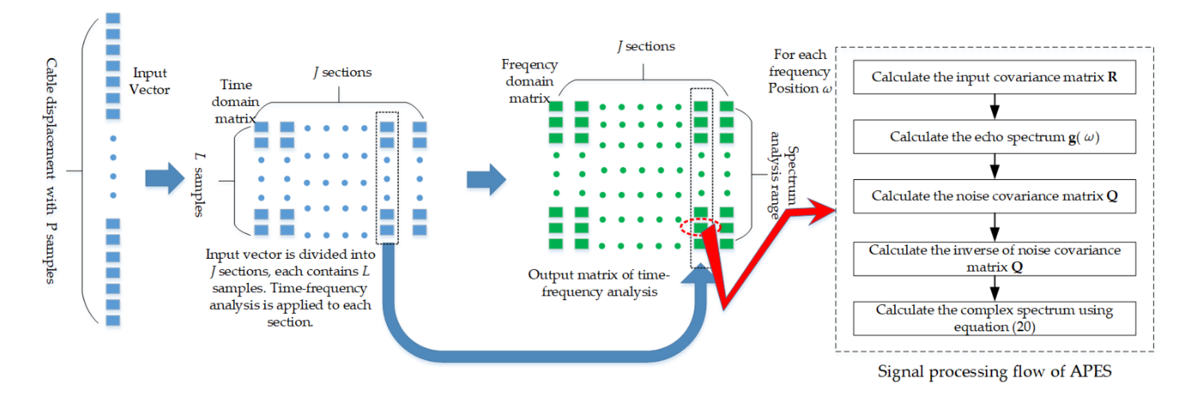
3.3. APES-Based Time-Frequency Analysis

If the dynamic cable-tension is the pursuit, the APES method can be applied repeatedly to different sections of the displacement vector. Nearby sections can be overlapped to get smoother results. The main signal processing flow of APES-based time-frequency analysis is similar to that of short-time Fourier transformation (STFT). The flow chart is shown in Figure 1.

• A long input displacement vector is filtered by a high-pass filter (HPF). The measured displacement always contains a DC offset component. There would be a large peak at 0 Hz in the spectrum. The sidelobe of the peak would be much larger than the peak of a cable’s fundamental frequency peak. So, a high-pass filter is used to suppress the adverse influence. There are many types of the HPF filter. The HPF filter in this manuscript is performed with a MATLAB function, called ‘smooth.’ The operation is formulated as $y(n)=d(n)-\mathrm{smooth}(d(n),L_{smooth})$. Where $L_{smooth}$ is the smooth length parameter of the ‘smooth’ function. The smaller the $L_{smooth}$, the larger the cut-frequency of the HPF filter. Then, the filtered displacement is decimated by a reasonable factor to reduce the total data length and the computation load subsequently.
• The new vector is divided into sections of the same length with some proper overlapping factors.
• Each section is processed by the APES algorithm.
• Frequency peaks from APES output are extracted. Fundamental frequency can be preliminarily identified if its high harmonic frequencies exist. Then, the fundamental frequencies are further judged, according to the relation that they are inversely proportional to the cable length.
• The APES algorithm and fundamental frequency identification are applied repeatedly to all the divided sections. Then the dynamic cable-tension can be obtained.

4. Results

In this section, the proposed method is evaluated by simulation and real interferometric radar data analysis.

4.1. Frequency Estimation Precision and Super-Resolution Ablility

Three simulation experiments are conducted to demonstrate the characters of APES. Two of them are to evaluate the frequency estimation precision under single-tone and double-tone conditions. The third one is to analyze the relations of estimation precision vs. SNR. Results reveal that the APES can achieve super-resolution ability and higher frequency estimation precision, especially in multi-tone circumstances. Parameters in these simulations are the same as those of the later K band interferometric radar.

Table 1. Parameters of APES in these simulations.

Vector Length ( s)	Frequency Resolution (Hz)	PRF (Hz)	Section Length (point)	Section Overlap (point)	Filter Taps (orders)	Spectrum Analysis Range (Hz)	Spectrum Analysis Interval (Hz)
10	0.1	20	200	180	100	0–5	0.000625

shows the parameters of APES in the following three simulations. The displacement sampling frequency is 20 Hz and the sampling length is 10 s. Therefore, the length of an input vector is 200 points. According to the time-frequency theory, the frequency resolution of the vector is ${\mathsf{\rho }}_f=1/10$ Hz. ZOOM-FFT (FFT for short), CZT, and APES methods are adopted to estimate the frequency. The spectrum analysis interval of these methods is set to ${\mathsf{\rho }}_f/160,$ which is fine enough to analyze the frequency resolution of the three methods. Stoica [18] suggests the APES filter tap to be half the input vector length to get an optimum result, so the filter tap is set to be 100 in the simulations.

By using the Monte Carlo method, each simulation is conducted 100 times. The mean absolute percentage error (MAPE) is used to assess the estimation precision. The MAPE is defined as:

$$\mathrm{\Delta }{f}_{MAPE}=\frac{1}{N_{sim}}{\displaystyle {\sum }_{i=1}^{N_{sim}}\left|\frac{f_i-f_{real}}{f_{real}}\right|}\times 100$$

(23)

where $f_i$ and $f_{real}$ are the estimated and the real frequency of the simulated tone, respectively. $N_{sim}$ is the repeated simulation number, and it is set to be 100.

4.1.1. Single-Tone Frequency Estimation

The first simulation aims to evaluate single-tone frequency estimation accuracy. The frequency of simulated sine waveform varies from 1.0 Hz to 2.0 Hz. A white Gauss noise with the −10 dB relative power is added to the single-tone waveform.

The curve of MAPE vs. frequency deviation is shown in Figure 2. The blue solid, red solid, and yellow dash curves are the results obtained by APES, FFT, and CZT, respectively. The red solid and yellow dash curves are overlapped, which indicates that the performances of FFT and CZT are the same. Since the blue and red curves are not always superior to each other, it can hardly judge which method is better. Since all the MAPE curves are lower than 0.025%, all three methods can achieve precise frequency estimation under the single-tone condition.

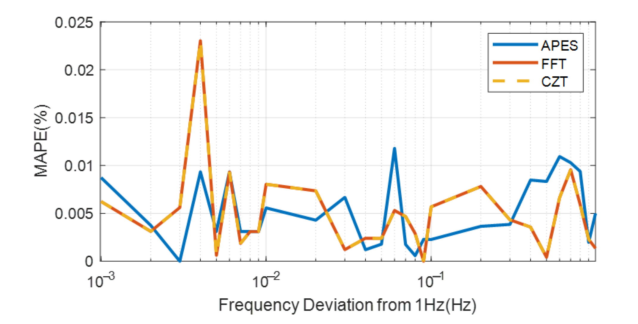
4.1.2. Double-Tone Signal Frequency Estimation

The second simulation aims to evaluate the frequency estimation performance when multiple tones are present, which is closer to the actual condition of a cable-tension measurement. The frequency of one tone is fixed at 1 Hz, and that of the other tone exponentially changes. The gap between the two tones ranges from 0.05 Hz, which is half the frequency resolution, to 3.97 Hz. A white Gauss noise whose power is −20 dB is added to the double-tone waveform.

The result of the second simulation is shown in Figure 3. The performances of the FFT and the CZT are also identical in this simulation. The MAPE curve of APES is much lower and keeps consistent among all the frequency gaps, even if the gap is below the resolution limit ${\mathsf{\rho }}_f$. This indicates the super-resolution ability of APES. However, the performances of FFT and CZT fluctuate. Their MAPEs are generally much larger and can reach some minimums only at specific frequency gaps. The reason for the phenomenon is that ZOOM-FFT and CZT are FFT-based methods and the Fourier transformation suffers sidelobe leakage. Both the estimation frequency of the fixed tone and the varying tones are contaminated by each other’s sidelobes. The simulation demonstrates that the performance of APES is superior to those of the two methods.

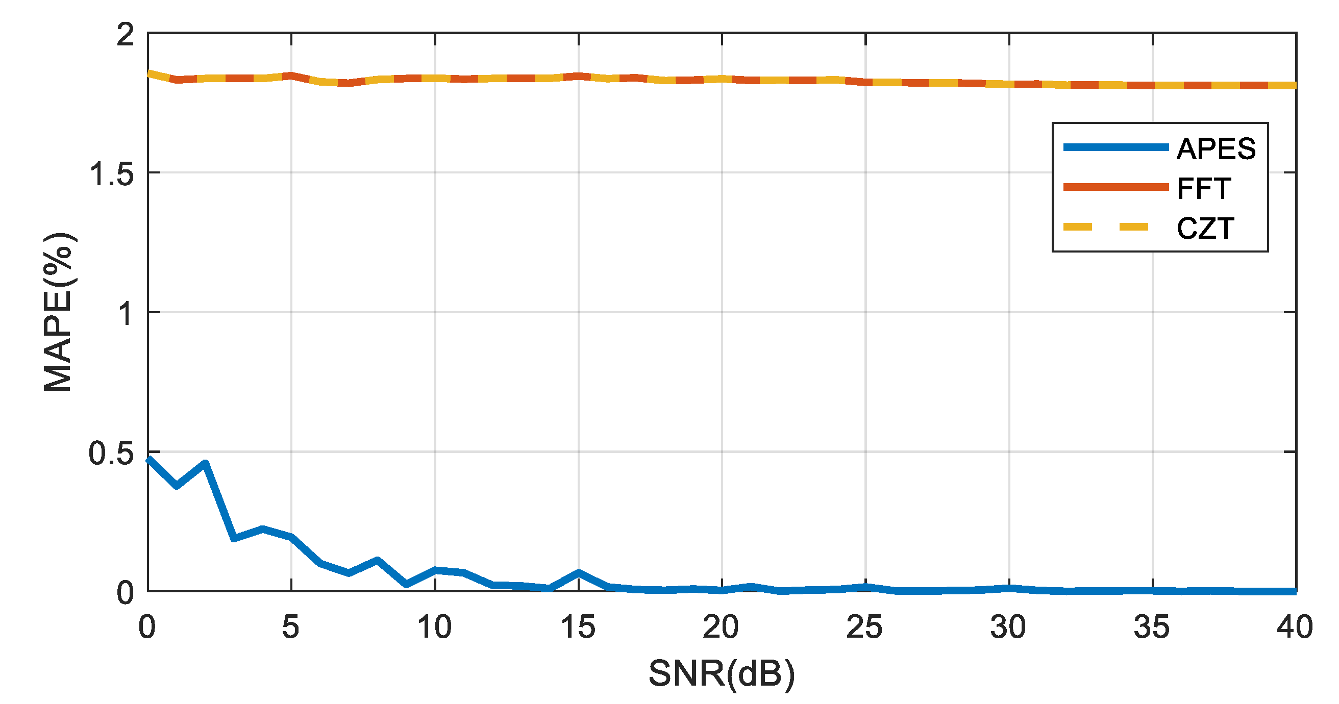
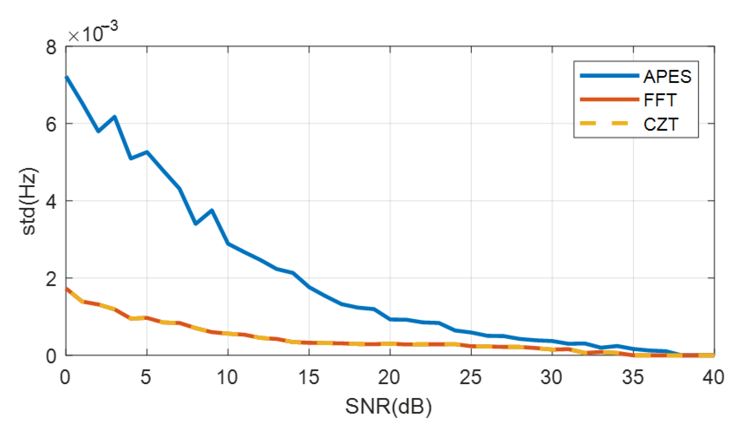
4.1.3. Frequency Estimation Performance vs. SNR

The third simulation aims to evaluate the frequency estimation robustness when the power of the added white Gauss noise varies from −40 dB to 0 dB at a 1 dB interval. The frequencies of the two tones are fixed at 1 Hz and 1.1 Hz. The gap equals the frequency resolution ${\mathsf{\rho }}_f$.

The MAPE and standard deviation(std) are chosen for comparison. The MAPE curves and the std curves are shown in Figure 4 and Figure 5, respectively. The curves of FFT and CZT are the same, so their performances are identical. Their MAPE curves are nearly constant with varying SNR levels, which indicates that the two methods are robust estimators. The MAPE curve of APES is much lower than those of the other two methods at all the SNR levels. At the same time, the MAPE curve of APES increases as SNR gets lower. Since APES is a data-dependent spectrum estimator, it is more affected by the level of input noise. The std curve of APES is generally larger than those of the other two methods. However, since the SNR is larger than 0 dB, it is the most common cable-tension estimation case. The APES methods can still achieve superior results.

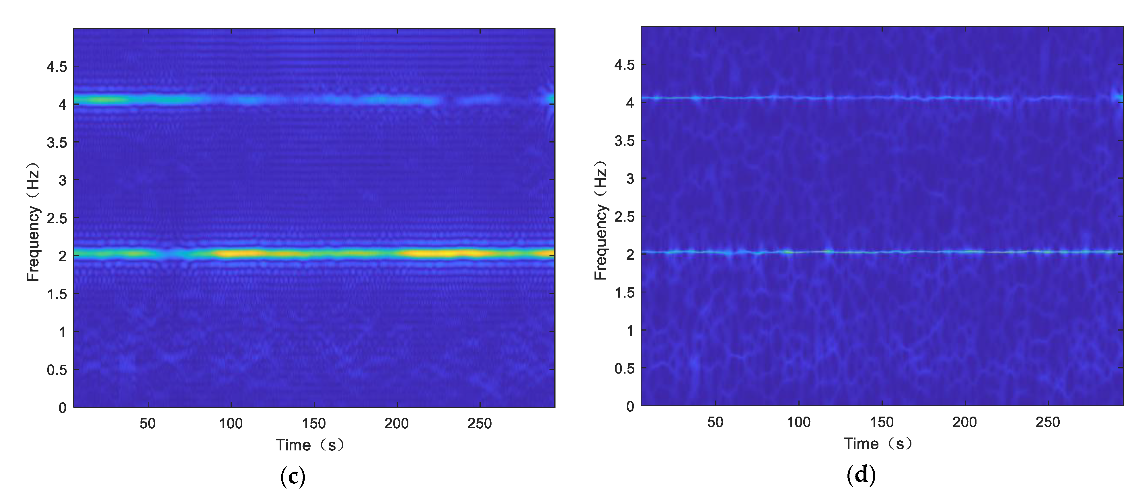
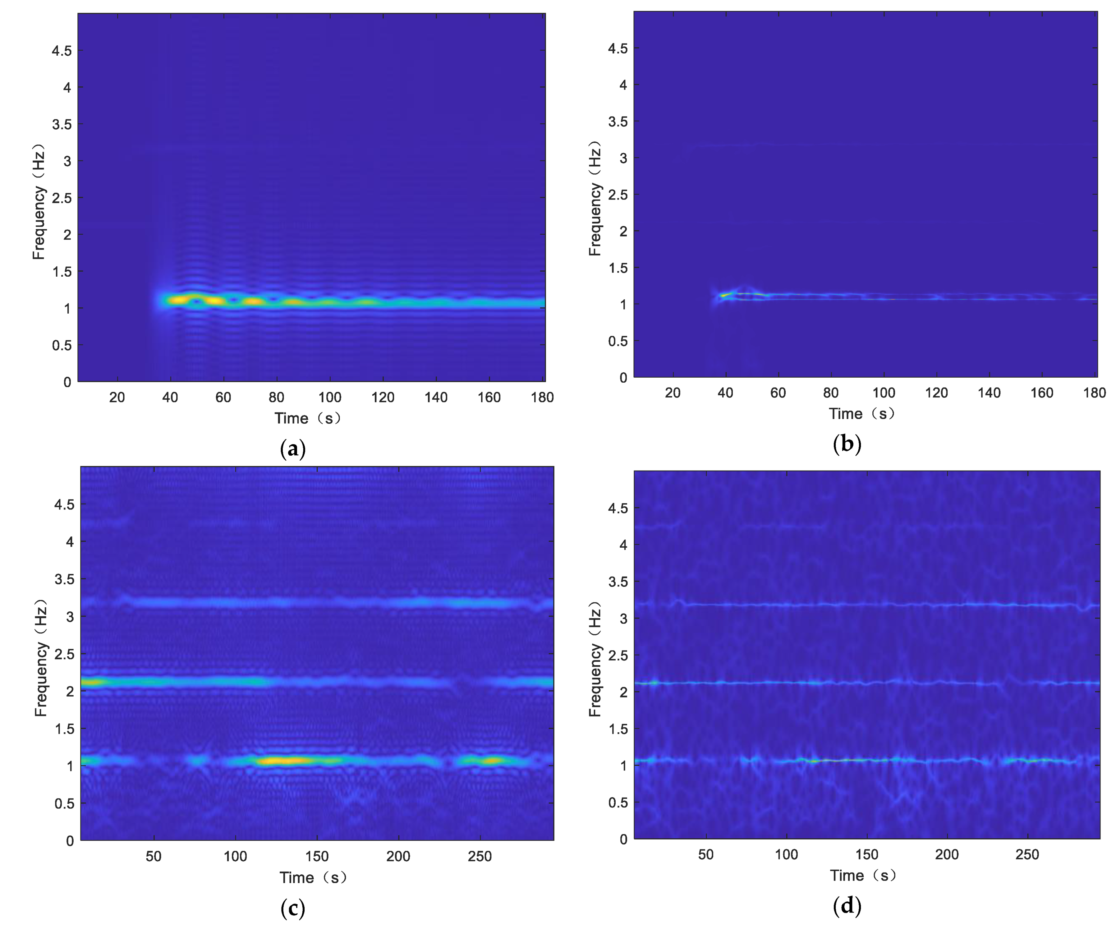
4.2. Dynamic Cable-Tension Analysis under the Impact of a High-Speed Train

The methods are applied to the data of a cable-stayed railway bridge. The bridge is 1 km south of the Changsha southern railway station. The bridge, which crosses the Wuguang high-speed railway line, is an import node of the Hukun high-speed railway line, as shown in Figure 6. It is composed of one tower and four groups of cables. Each group contains 8 cables. Its tower height is 72.9 m and its span length is 224 m. An interferometric radar is placed by the foot of the tower to measure the cables. The radar is a pointed ramp upwards to make sure that cables are within the beam width of the antennas. The picture of the interferometric used in the experiment is placed at the lower-left corner. The antennas used in this experiment are horn antennas, and their beam width are about $15°\times 15°$. Due to the block of the bridge body, the five longest cables are visible to the radar. The parameters of the radar are listed in

Table 2. Parameters of simulation and the K band interferometric radar.

Frequency Range	Band Width (GHz)	Sampling Frequency (MHz)	Antenna Gain (dBi)	Transmitting Power (dBmW)	PRF (Hz)	Decimate Factor
K band	1	10	22	27	200	10:1

. We recorded their displacements at 200 Hz for 186 s during which a train passed by. We also recorded their displacements without passing trains for comparison and the duration of the recorded data is 300 s.

Figure 7 shows the radar image of the experimental scene. We can see the five peaks marked by blue dash lines correspond to the five cables. These cables are the ones in a red color in Figure 6. Their displacement curves are shown in Figure 8. These curves vibrate within small ranges, then change immediately when the train enters the bridge, and remain vibrating with much larger amplitudes when the train leaves the bridge. These cables under changing ambient load may bear changing force. Dynamic cable-tension is estimated by the APES method and the CZT method. Only the nearest and farthest cable is analyzed to make the article concise. The time-frequency distribution images of the two cables are shown in Figure 9 and Figure 10. The spectrum obtained by APES has much sharper peaks and lower sidelobe in both experiments. The APES method can resolve the two frequencies around 1.1 Hz that the CZT method cannot do in Figure 10. The superior performance of APES is prominent in these experiments.

Time-frequency distribution is an important approach to analyze cable’s dynamic character. There are three bright lines in Figure 9a,b, and two bright lines in Figure 9c,d. The extra line around 1 Hz is the fundamental frequency of the bridge deck, which is excited by the passing train after 35 s. The component can be observed in all cable’s time-frequency distribution images. At other times, the displacement of the bridge deck is trivial, so its fundamental frequency can hardly be observed. When the fundamental frequency components of the deck and the shortest cable are separated with a large interval, in Figure 9a,b, both the CZT and the APES methods can give good results. On the contrary, the fundamental frequency of the deck and the longest cable are adjacent in Figure 10a,b. Only the APES can distinguish them. The two frequency components of the shortest cable are observed in the interval between 0 Hz to 5 Hz in Figure 9. At the same time, four frequency components of the longest cable are observed.

By the analysis tools, dynamic behaviors of the bridge can be observed and analyzed. The fundamental frequency is extracted from the time-frequency distribution images in Figure 9 and Figure 10. The fundamental frequency curves are shown in Figure 11. The results of APES and CZT are displayed as blue lines and red lines, respectively. Some significant details of the dynamic fundamental frequency are observed.

• When the frequency of interest is far from other frequency components, both methods can obtain similar estimation performance. The curves in Figure 11b,d and before 30 s in Figure 11a,c are the cases.
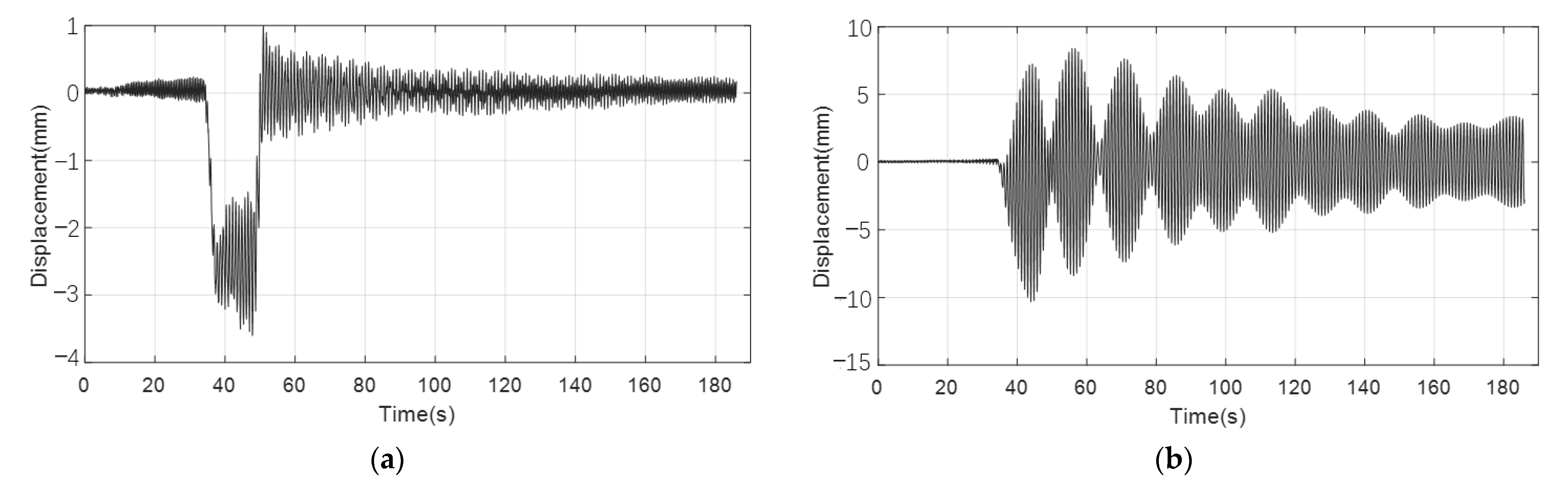
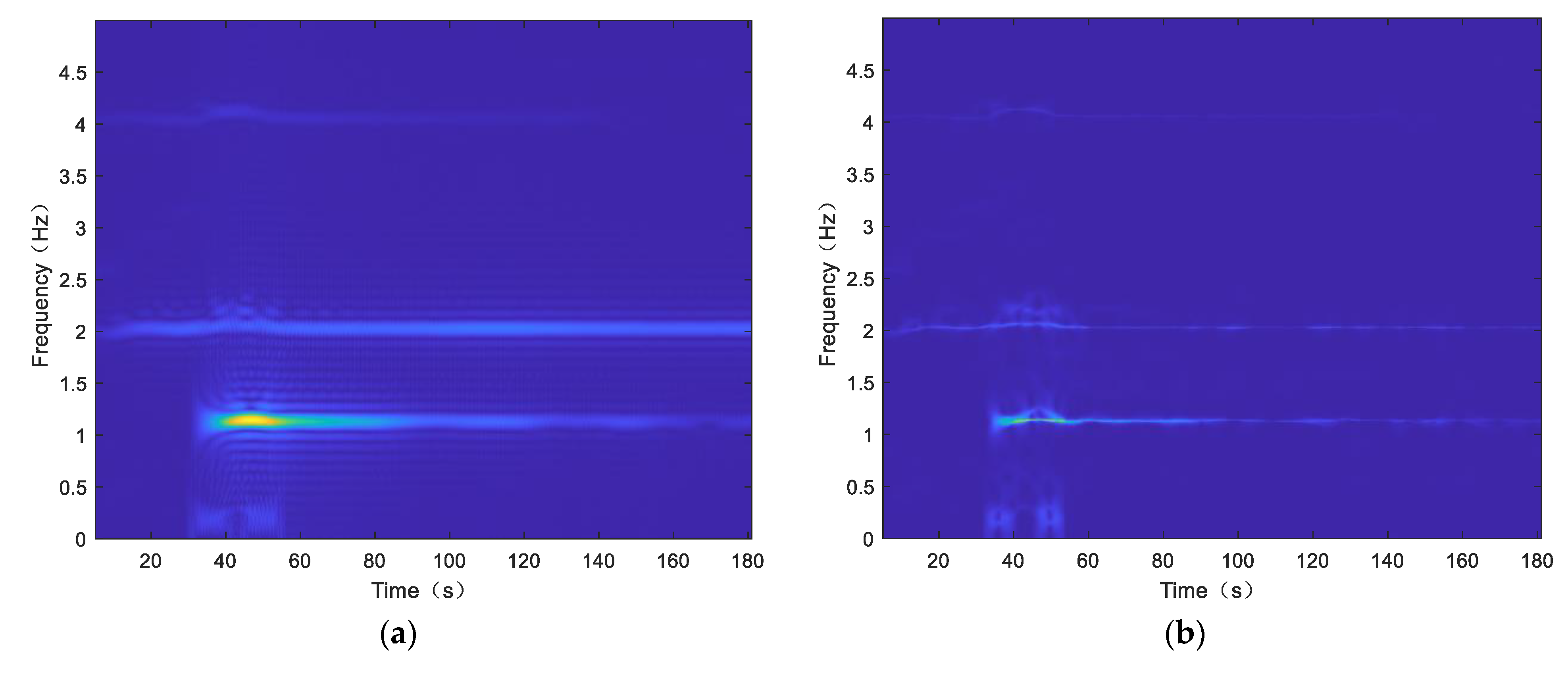
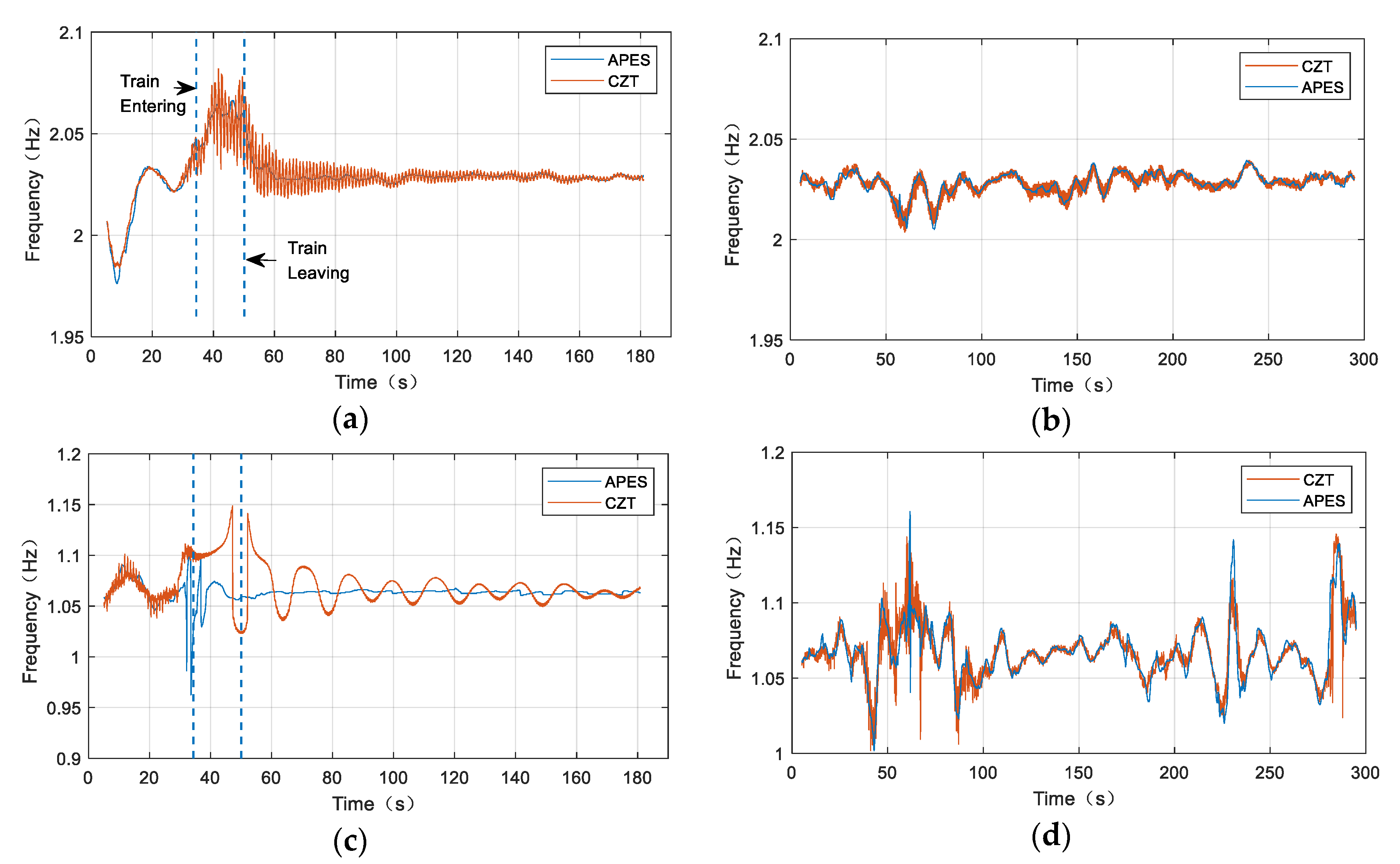
• When the frequency of interest is interfered by a nearby frequency component, the CZT method suffers fluctuated estimation. The smaller the frequency gap, the larger the fluctuating amplitude. Fortunately, the APES method can still achieve fine estimation. The curves after 50 s in Figure 11a,c are the cases.
• When the train embarks the bridge, the fundamental frequency increases. This means that the cable-tension increases. The increased tension phenomenon is observed in all the cables, so it is feasible to calculate the bridge load from the sum of all cables’ tension.
• The fundamental frequency curve in Figure 11a is complicated a short moment before the train enters the bridge. The cable-tension undergoes a decreasing and then increasing progress.
• Dynamic frequency estimation is also a challenge for the APES method, especially when the frequency component is not a stationary sinusoidal signal and be interfered by closely signals. This is the reason that the frequency curve of APES changes rapidly, in Figure 11c.

By taking a look at the spectrum slices of the two methods, in Figure 12, we know why the CZT method outputs fluctuated frequency estimation. The slices are taken at the moment of 47.1 s, 47.2 s, and 47.3 s. The frequency peaks of the APES method are constant, but the peaks of the CZT method are not always distinguished. The CZT method would find a correct peak at 47.3 s, but wrong peaks at 47.1 s and 47.2 s.

5. Conclusions

A remote dynamic cable-tension estimation method is presented. Displacements of a group of cables are measured by a K band interferometry radar at one time. Each cable-tension can be calculated from the cable’s fundamental frequency, based on the string vibration equation. By adopting a time-frequency analysis method, multiple fundamental frequencies are estimated from short sections of the entire measured displacement vector in an overlapped-piecewise manner. The amplitude and phase estimation (APES) algorithm is used to improve the frequency estimation performance in short-time circumstances. Simulations and real data processing validate that the proposed method is superior to traditional fundamental frequency measurements in terms of precision, robustness, and efficiency.

The proposed interferometry radar and signal processing method can give remote, efficient, precise, and dynamic fundamental frequency measurements. It is of great application value in the bridge construction control stage, the bridge operation monitoring stage, and the bridge refinement stage. The APES algorithm is a vital part of the proposed method, and its execution efficiency needs to be further improved. This is a research direction in the future.

References

1. List of Longest Bridges. Available online: https://en.wanweibaike.com/wiki-World’s%20longest%20bridge (accessed on 22 September 2020).
2. Hassan, M.; Nassef, A.; El Damatty, A. Surrogate function of post-tensioning cable forces for cable-stayed bridges. Adv. Struct. Eng. 2013, 16, 559–578. [Google Scholar] [CrossRef]
3. Wu, M.; Tang, D.; Cheng, M. Research of Cable-tension Sensor with Bypass Excitation Structure Based on Magneto-elastic Effect in Cable-stayed Bridge. In Proceedings of the World Congress on Intelligent Control & Automation, Chongqing, China, 25–27 June 2008; pp. 7560–7563. [Google Scholar]
4. Kim, B.; Park, T. Estimation of cable-tension force using the frequency-based system identification method. J. Sound Vib. 2007, 304, 660–676. [Google Scholar] [CrossRef]
5. Zhao, Z.; Sun, J.; Fei, X.; Liu, W.; Cheng, X.; Wang, Z.; Yang, H. Wireless Sensor Network Based Cable-tension Monitoring for Cable-stayed Bridges. In Proceedings of the 2012 14th International Conference on Advanced Communication Technology (ICACT), Pyeongchang, Korea, 19–22 February 2012; pp. 527–532. [Google Scholar]
6. Shao, Z.; Zhang, X.; Li, Y.; Jiang, J. A Comparative Study on Radar Interferometric for Vibrations Monitoring on Different Types of Bridges. IEEE Access 2018, 6, 29677–29684. [Google Scholar] [CrossRef]
7. Gentile, C. Application of microwave remote sensing to dynamic testing of stay-cables. Remote Sens. 2010, 2, 36–51. [Google Scholar] [CrossRef] [Green Version]
8. Dong, H.; Wang, J.; Song, Q. A way of cable force measurement based on interference radar. In Proceedings of the Electromagnetic Research Symposium (PIERS), Shanghai, China, 8–11 August 2016. [Google Scholar]
9. Zhao, W.; Zhang, G.; Zhang, J. Cable force estimation of a long-span cable-tayed bridge with microwave interferometric radar. Comput. Aided Civ. Infrastruct. Eng. 2020, 35, 1419–1433. [Google Scholar] [CrossRef]
10. Gentile, C.; Bernardini, G. An interferometric radar for non-contact measurement of deflections on civil engineering structures: Laboratory and full-scale tests. Struct. Infrastruct. Eng. 2010, 6, 521–534. [Google Scholar] [CrossRef]
11. Mehrabi, A.B.; Tabatabai, H. A unified finite difference formulation for free vibration of cables. J. Struct. Eng. ASCE 1998, 124, 1313–1322. [Google Scholar] [CrossRef]
12. Su, D.; Tu, Y.; Ming, L.; Li, J. Comparative analysis of frequency estimation methods. In Proceedings of the 31st Chinese Control Conference, Hefei, China, 25–27 July 2012; pp. 5442–5447. [Google Scholar]
13. Park, S.Y.; Song, Y.S.; Kim, H.J.; Park, J. Improved method for frequency estimation of sampled sinusoidal signals without iteration. IEEE Trans. Instrum. Meas. 2011, 60, 2828–2834. [Google Scholar] [CrossRef]
14. Giarnetti, S.; Leccese, F.; Caciotta, M. Non recursive nonlinear least squares for periodic signal fitting. Meas. J. Int. Meas. Confed. 2017, 103, 208–216. [Google Scholar] [CrossRef]
15. Spagnolo, G.S.; Cozzella, L.; Leccese, F. Phase correlation functions: FFT vs. FHT. Acta IMEKO 2019, 8, 87–92. [Google Scholar] [CrossRef]
16. Li, J.; Stoica, P.; Wang, Z. On robust Capon beamforming and diagonal loading. IEEE Trans. Signal Process. 2003, 51, 1702–1715. [Google Scholar]
17. Li, J.; Stoica, P. An adaptive filtering approach to spectral estimation and SAR imaging. IEEE Trans. Signal Process. 1996, 44, 1469–1484. [Google Scholar]
18. Stoica, P.; Li, H.; Li, J. A new derivation of the APES filter. IEEE Signal Processing Letters, Aug. 1999, 6, 205–206. [Google Scholar] [CrossRef]
19. Liu, Z.; Li, H.; Li, J. Efficeint implementation of Capon and APES for spectral estimation. IEEE Trans. AES 1998, 34, 1314–1319. [Google Scholar]
20. Larsson, E.; Stoica, P. Fast implementation of two-dimensional APES and Capon spectral estimators. Multidimens. Syst. Signal Process. 2002, 13, 35–54. [Google Scholar] [CrossRef]
21. Glentis, G. A Fast Algorithm for APES and Capon Spectral Estimation. IEEE Trans. GRS 2008, 56, 4207–4220. [Google Scholar] [CrossRef]
22. Knott, E.F.; Shaeffer, J.F.; Tuley, M.T. Radar Cross Section, 2nd ed.; Scitech Publishing, Inc.: Raleigh, NC, USA, 2004; pp. 195–196. [Google Scholar]
23. Sarabandi, K.; Park, M. Millimeter-wave radar phenomenology of power lines and a polarimetric detection algorithm. IEEE Trans. Antennas Propag. 1999, 47, 1807–1813. [Google Scholar] [CrossRef] [Green Version]
Figure 1. Time-frequency analysis flow charts of a bridge cable.
Electronics 10 00501 g001
Figure 2. Single-tone frequency estimation error vs. different frequency position. The blue solid curve, the red solid curve, and the yellow dash curve are the results obtained by adaptive amplitude and phase estimation (APES), fast Fourier transform (FFT), and chirp z-transform (CZT), respectively.
Electronics 10 00501 g002
Figure 3. Double-tone frequency estimation error vs. different frequency position. The blue solid curve, the red solid curve, and the yellow dash curve are the results obtained by APES, FFT, and CZT, respectively.
Electronics 10 00501 g003
Figure 4. Mean absolute percentage error (MAPE) vs. different signal to noise ratio (SNR). The blue solid curve, the red solid curve, and the yellow dash curve are the results obtained by APES, FFT, and CZT, respectively.
Electronics 10 00501 g004
Figure 5. Standard deviation of frequency estimation error vs. different SNR. The blue solid curve, the red solid curve, and the yellow dash curve are the results obtained by APES, FFT, and CZT, respectively.
Electronics 10 00501 g005
Figure 6. Experimental descriptions. The Hukun-Wuguang bridge is on the south of the southern Changsha railway station. The five longer cables on the north-east side are measured.
Electronics 10 00501 g006
Figure 7. High resolution 1D radar image of the five cables. The five peaks are among 45 m to 70 m, which correspond to the five longest cables in a red color in Figure 6.
Electronics 10 00501 g007
Figure 8. The cable displacements of the Hukun-Wuguang bridge, which (a) is the displacement of the nearest cable at 52.19 m and (b) is the displacement of the farthest cable at 67.02 m.
Electronics 10 00501 g008
Figure 9. Time-frequency distribution of the shortest cable. (a) result of CZT-based short-time Fourier transformation (STFT) and (b) result of APES-based time-frequency distribution, when a train passes by for 35 s and 40 s. (c) Result of CZT-based STFT and (d) result of APES-based time-frequency distribution, when the bridge is on a free condition.
Electronics 10 00501 g009aElectronics 10 00501 g009b
Figure 10. Time-frequency distribution of the longest cable. (a) Result of CZT-based STFT and (b) result of APES-based time-frequency distribution, when a train passes by for 35 s and 40 s. (c) The result of CZT-based STFT and (d) result of APES-based time-frequency distribution, when the bridge is on a free condition.
Electronics 10 00501 g010
Figure 11. Fundamental frequency curves extracted from the time-frequency distribution images. The blue curve and the red curve are results of the CZT and the APES method, respectively. Dynamic fundamental frequency of the shortest cable with the passing train (a) and without load (b). Dynamic fundamental frequency of the longest cable with the passing train (c) and without load (d).
Electronics 10 00501 g011
Figure 12. Spectrum slices of the CZT method at a different time (blue solid line at 47.1 s, red solid line at 47.2 s, and orange solid line at 47.3 s). Spectrum slices of the APES method at different times are constant.
Electronics 10 00501 g012